1 中華大學資訊工程學系 http:// ching-hsien hsu ( 許慶賢 ) localization and scheduling...
TRANSCRIPT

1中華大學資訊工程學系 http:// www.csie.chu.edu.tw
Ching-Hsien Hsu ( 許慶賢 )
Localization and Scheduling Techniques for
Optimizing Communications on Heterogeneous
Cluster Grid

2
Outline
IntroductionRegular / Irregular Data Distribution, RedistributionCategory of Runtime Redistribution Problems
Processor Mapping Technique for Communication Localization
The Processor Mapping TechniqueLocalization on Multi-Cluster Grid System
Scheduling Contention Free Communications for Irregular Problems
The Two-Phase Degree Reduction Method (TPDR)Extended TPDR (E-TPDR)
Conclusions
3
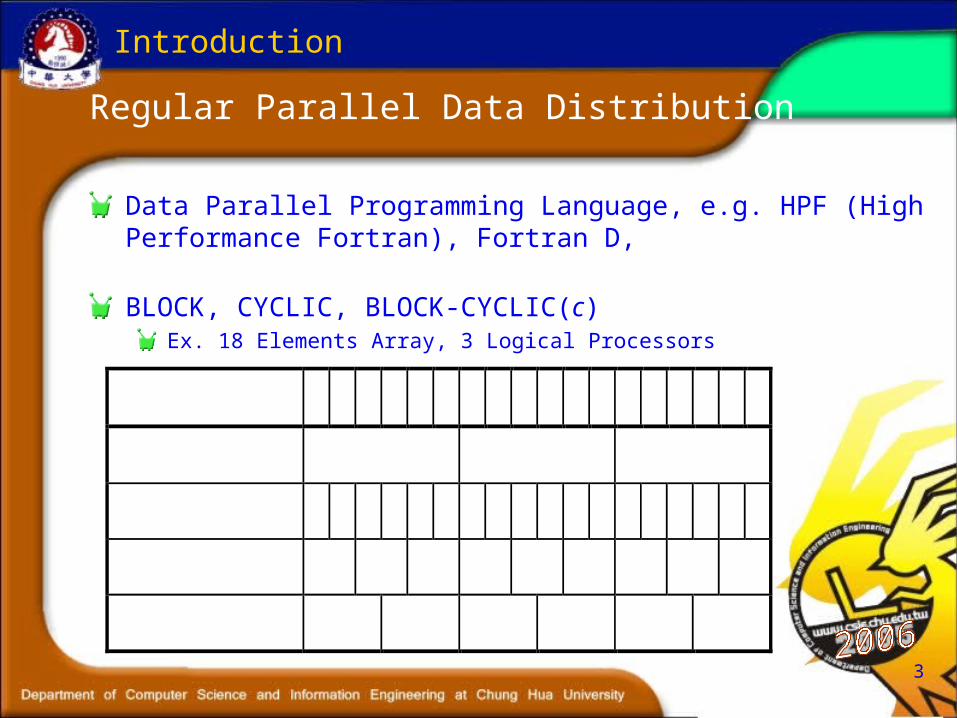
Regular Parallel Data Distribution
Data Parallel Programming Language, e.g. HPF (High Performance Fortran), Fortran D,
BLOCK, CYCLIC, BLOCK-CYCLIC(c)Ex. 18 Elements Array, 3 Logical Processors
global-index 1 2 3 4 5 6 7 8 9 10 11 12 13 14 15 16 17 18
block P0 P1 P2
cyclic P0 P1 P2 P0 P1 P2 P0 P1 P2 P0 P1 P2 P0 P1 P2 P0 P1 P2
block-cyclic(2) P0 P1 P2 P0 P1 P2 P0 P1 P2
block-cyclic(3) P0 P1 P2 P0 P1 P2
Introduction

4
Two Dimension Matrices
Introduction (cont.)
8 8 matrix (BLOCK, BLOCK) onto P(2, 2) (CYCLIC, *)
onto P(4, *) (CYCLIC(2), BLOCK) onto P(2, 2)
Data Distribution

5
Data Redistribution
Introduction (cont.)
Processor Rank
Local index
0 1 2 0 1 2 0 1 2
1 2 1 2 1 2 3 4 3 4 3 4 1 2 3 4 1 2 3 4 1 2 3 4
1 1
20
2 P0 P1 P20
3P0 P1 P2 P0 P1 P2
1
11
2 P3 P4 P5
2 113
P3 P4 P5 P3 P4 P5 02 P0 P1 P2
4 3
51
4 P3 P4 P50
6P0 P1 P2 P0 P1 P2
3
40
4 P0 P1 P2
5 316
P3 P4 P5 P3 P4 P5
14 P3 P4 P5
Source: (BC(3), BC(2)) Destination: (BC(2), BC(4))

6
Data Redistribution
Introduction (cont.)
REAL DIM(18, 24) :: A!HPF$ PROCESSORS P(2, 3)!HPF$ DISTRIBUTE A(BLOCK, BLOCK) ONTO P
: (computation)
!HPF$ REDISTRIBUTE A(CYCLIC, CYCLIC(2)) ONTO P: (computation)

7
Irregular Redistribution
Introduction (cont.)
PARAMETER (S = /7, 16, 11, 10, 7, 49/)
!HPF$ PROCESSORS P(6)
REAL A(100), new (6)
!HPF$ DISTRIBUTE A (GEN_BLOCK(S)) onto P
!HPF$ DYNAMIC
new = /15, 16, 10, 16, 15, 28/
!HPF$ REDISTRIBUTE A (GEN_BLOCK(new))
8
Introduction (cont.)
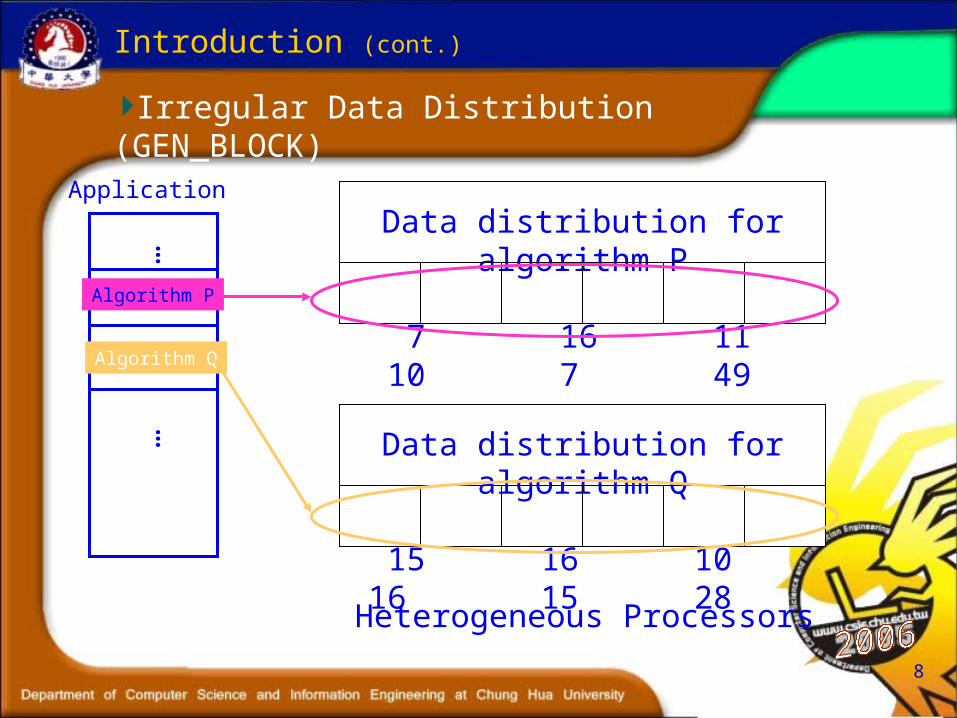
Irregular Data Distribution (GEN_BLOCK)
Data distribution for algorithm P
7 16 11 10 7 49
Data distribution for algorithm Q
15 16 10 16 15 28
Application
……
Algorithm P
Algorithm Q
Heterogeneous Processors
9
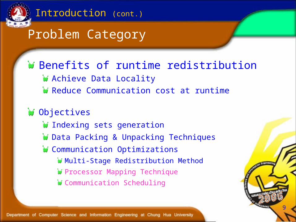
Problem Category
Benefits of runtime redistributionAchieve Data LocalityReduce Communication cost at runtime
ObjectivesIndexing sets generation
Data Packing & Unpacking Techniques
Communication OptimizationsMulti-Stage Redistribution Method
Processor Mapping Technique
Communication Scheduling
Introduction (cont.)

10
Outline
IntroductionRegular / Irregular Data Distribution, RedistributionCategory of Runtime Redistribution Problems
Processor Mapping Technique for Communication Localization
The Processor Mapping TechniqueMulti-Cluster Grid System
Contention Free Communication Scheduling for Irregular Problems
The Two-Phase Degree Reduction Method (TPDR)Extended TPDR (E-TPDR)
Conclusions

11
The Original Processor Mapping Technique (Prof. Lionel. M. Ni)
Mapping function is provided to generate a new sequence of logical processor id
Increase data hits
Minimize the amount of data exchange
Processor Mapping Technique

12
An Optimal Processor Mapping Technique(Hsu’05)
Example: BC86 over 11
Traditional Method Size Oriented Greedy Matching Maximum Matching (Optimal)
Processor Mapping Technique (cont.)

13
Localize communications
Cluster GridInterior CommunicationExternal Communication
Processor Mapping Technique (cont.)
node1
node3
node2
node4
node1
node3
node2
.node4
node1
.node3
node2
node4
node1
.node3
node2
.node4
node1
node3
node2
node4
14
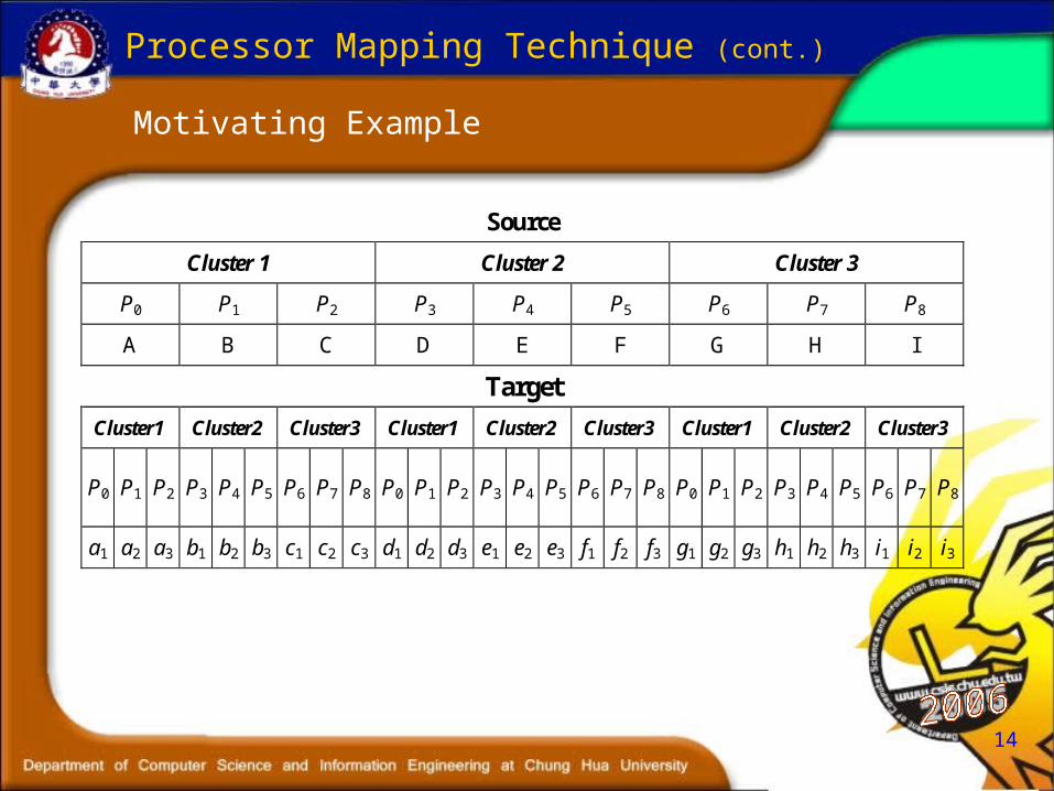
Motivating Example
Processor Mapping Technique (cont.)
Source
Cluster 1 Cluster 2 Cluster 3
P0 P1 P2 P3 P4 P5 P6 P7 P8
A B C D E F G H I
Target
Cluster1 Cluster2 Cluster3 Cluster1 Cluster2 Cluster3 Cluster1 Cluster2 Cluster3
P0 P1 P2 P3 P4 P5 P6 P7 P8 P0 P1 P2 P3 P4 P5 P6 P7 P8 P0 P1 P2 P3 P4 P5 P6 P7 P8
a1 a2 a3 b1 b2 b3 c1 c2 c3 d1 d2 d3 e1 e2 e3 f1 f2 f3 g1 g2 g3 h1 h2 h3 i1 i2 i3

15
Communication Table Before Processor Mapping
Processor Mapping Technique (cont.)
DP
SP P0 P1 P2 P3 P4 P5 P6 P7 P8
P0 a1 a2 a3
P1 b1 b1 b2
P2 c1 c2 c3
P3 d1 d2 d3
P4 e1 e2 e3
P5 f1 f2 f3
P6 g1 g1 g2
P7 h1 h2 h3
P8 i1 i2 i3
Cluster 1 Cluster 2 Cluster 3
|I|=9 |E|=18

16
Communication links Before Processor Mapping
Processor Mapping Technique (cont.)
Source
P0 P1 P2 P3 P4 P5 P6 P7 P8
P0 P1 P2 P3 P4 P5 P6 P7 P8
Target
Interior communication
External communication
17
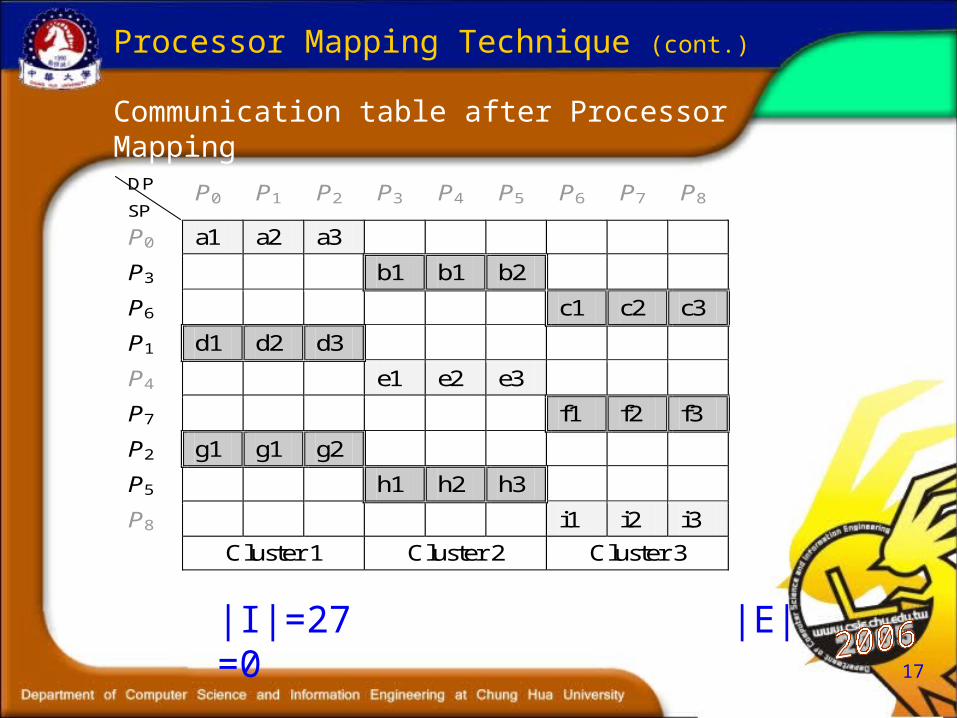
Communication table after Processor Mapping
Processor Mapping Technique (cont.)
DP
SP P0 P1 P2 P3 P4 P5 P6 P7 P8
P0 a1 a2 a3
P3 b1 b1 b2
P6 c1 c2 c3
P1 d1 d2 d3
P4 e1 e2 e3
P7 f1 f2 f3
P2 g1 g1 g2
P5 h1 h2 h3
P8 i1 i2 i3
Cluster 1 Cluster 2 Cluster 3
|I|=27 |E|=0
18
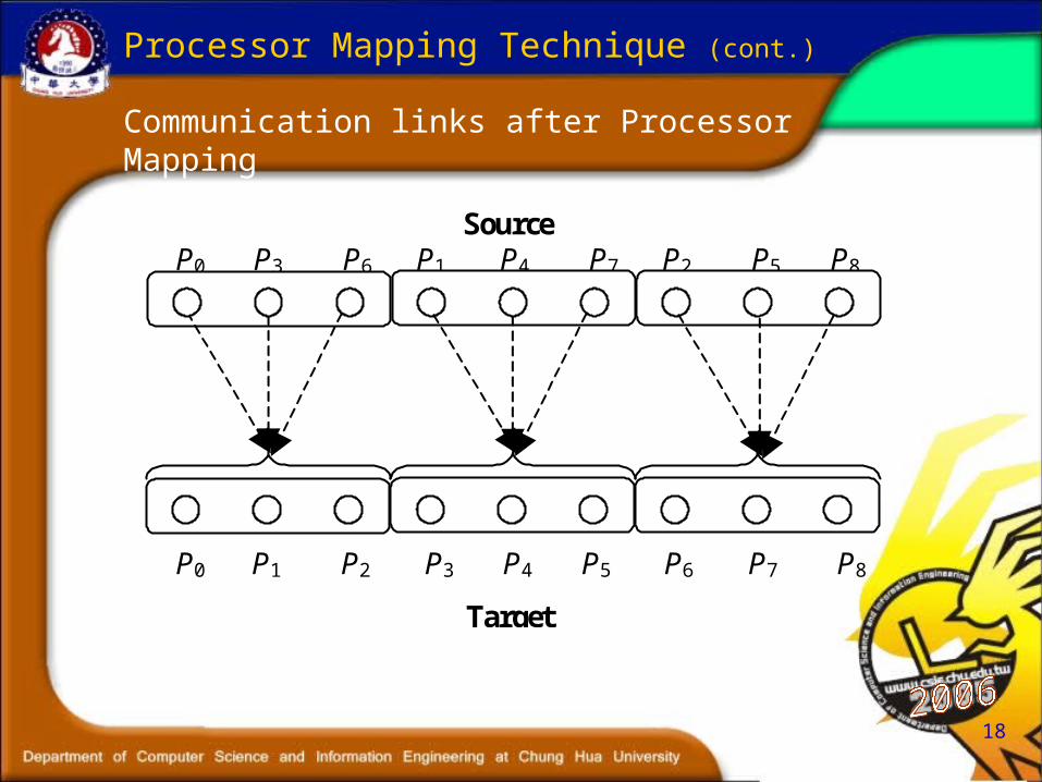
Communication links after Processor Mapping
Processor Mapping Technique (cont.)
Source P0 P3 P6 P1 P4 P7 P2 P5 P8
P0 P1 P2 P3 P4 P5 P6 P7 P8
Target

19
Processor Reordering Flow Diagram
Processor Mapping Technique (cont.)
Mapping Function
Partitioning Data
Alignment/Dispatch
Source Data
Reordering Agent
SCA(x)
Generate new Pid
Reordering SD(Px’)
DCA(x)
Determine Target Cluster
Designate Target Node
SCA(x)SCA(x)
SD(Px)
Master Node
DCA(x)DCA(x)DD(Py)
F(X) = X’ = +(X mod C) * K

20
Identical Cluster Grid vs. Non-identical Cluster Grid
Processor Mapping Technique (cont.)
DP
SP P0 P1 P2 P3 P4 P5 P6 P7 P8 P9 P10 P11
P0 a1 a2 a3 a4
P1 b1 b2 b3 b4
P2 c1 c2 c3 c4
P3 d1 d2 d3 d4
P4 e1 e2 e3 e4
P5 f1 f2 f3 f4
P6 g1 g2 g3 g4
P7 h1 h2 h3 h4
P8 i1 i2 i3 i4
P9 j1 j2 j3 j4
P10 k1 k2 k3 k4
P11 l1 l2 l3 l4
Cluster-1 Cluster-2 Cluster-3 Cluster-4
DP
SP P0 P1 P2 P3 P4 P5 P6 P7 P8 P9 P10 P11 P12 P13
P0 a1 a2 a3 a4 a5
P1 b1 b2 b3 b4 b5
P2 c5 c1 c2 c3 c4
P3 d1 d2 d3 d 4 d 5
P4 e1 e2 e3 e4 e5
P5 f4 f5 f1 f2 f3
P6 g1 g2 g3 g4 g5
P7 h1 h2 h3 h4 h5
P8 i3 i4 i5 i1 i2
P9 j1 j2 j3 j4 j5
P10 k1 k2 k3 k4 k5
P11 l2 l3 l4 l5 l1
P12 m1 m2 m3 m4 m5
P13 n1 n2 n3 n4 n5
Cluster1 Cluster2 Cluster3 Cluster4
21
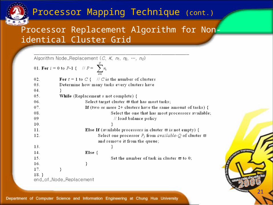
Processor Replacement Algorithm for Non-identical Cluster Grid
Processor Mapping Technique (cont.)
22
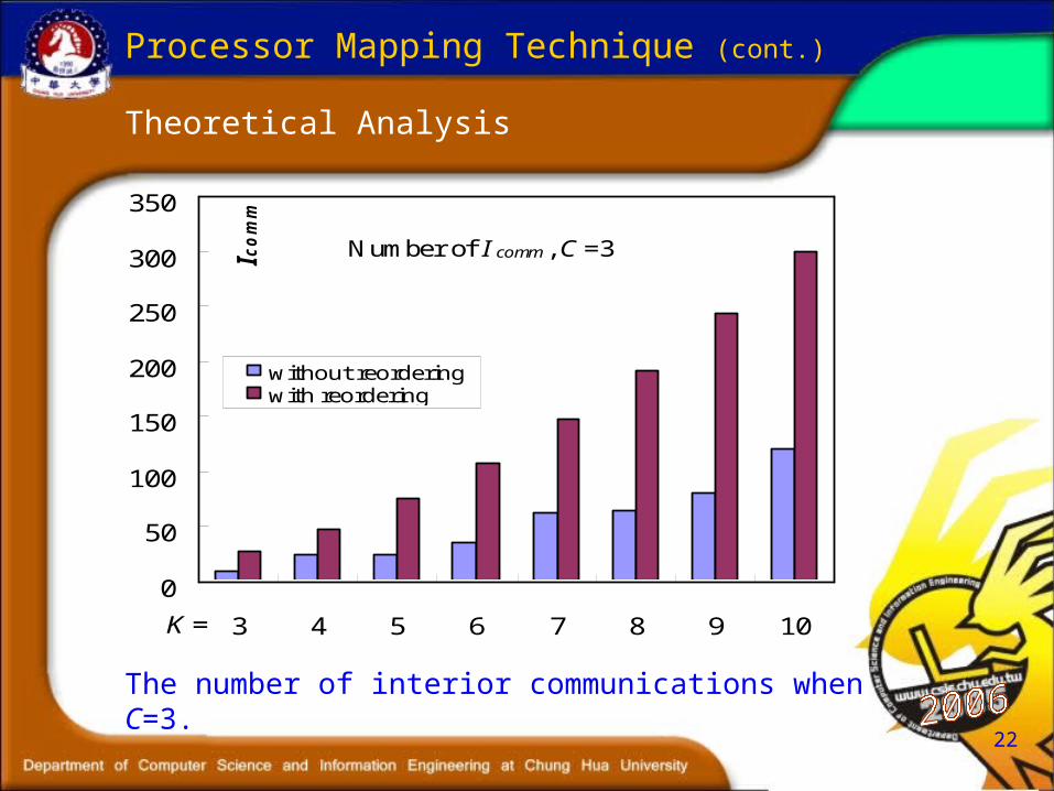
Theoretical Analysis
Processor Mapping Technique (cont.)
Number of I comm , C =3
0
50
100
150
200
250
300
350
3 4 5 6 7 8 9 10K =
I com
m
without reorderingwith reordering
The number of interior communications when C=3.
23
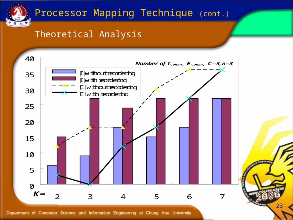
Theoretical Analysis
Processor Mapping Technique (cont.)
Number of Icomm, Ecomm, C=3,n=3
0
5
10
15
20
25
30
35
40
2 3 4 5 6 7K=
|I| without reordering|I| with reordering|E| without reordering|E| with reordering

24
Theoretical Analysis
Processor Mapping Technique (cont.)
C=4, (n1, n2, n3, n4)=(2, 3, 4, 5)
0
10
20
30
40
50
60
2 3 4 5 6 7 8 9 10
K
|I|
Original
Reordering A
Reordering B

25
Simulation Setting
Processor Mapping Technique (cont.)
Taiwan UniGrid
8 campus clusters
SPMD Programs
C+MPI codes.

26
Topology
Processor Mapping Technique (cont.)
Tainan
Taichung
Academia SinicaAcademia SinicaNational Tsing Hua University1
National Tsing Hua University1
Taipei
Hsing Kuo University
Hsing Kuo University
Chung Hua UniversityChung Hua University
National Center for High-performance ComputingNational Center for High-performance Computing
National Tsing Hua University2National Tsing
Hua University2
National Dong Hwa University National Dong Hwa University
Hsinchu
Hualien Providence UniversityProvidence University
Tunghai University
Tunghai University

27
Hardware Infrastructure
Processor Mapping Technique (cont.)
HKUIntel P3 1.0, 256M
THUDual AMD 1.6, 1G
CHUIntel P4 2.8, 256M
SINICADual Intel P3 1.0, 1G
NCHCDual AMD 2000+, 512M
PUAMD 2400+, 1G
NTHUDual Xeon 2.8, 1G
NDHUAMD Athlon, 256M
InternetInternet
28
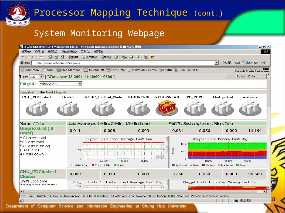
System Monitoring Webpage
Processor Mapping Technique (cont.)
29
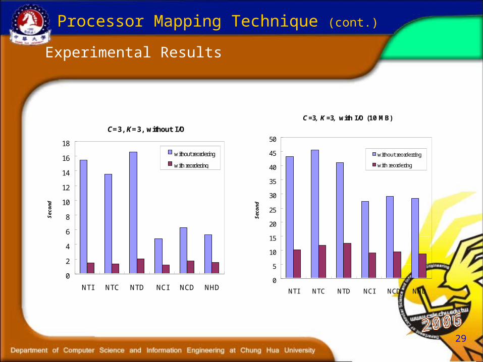
Experimental Results
C=3, K=3, without I/O
0
2
4
6
8
10
12
14
16
18
NTI NTC NTD NCI NCD NHD
Sec
ond
without reordering
with reordering
Processor Mapping Technique (cont.)
C=3, K=3, with I/O (10 MB)
0
5
10
15
20
25
30
35
40
45
50
NTI NTC NTD NCI NCD NHD
Sec
ond
without reorderring
with reordering

30
Experimental Results
Processor Mapping Technique (cont.)
Label Organization
N National Center for High Performance Computing
T National Tsing Hua University
C Chung Hua University
H Tung Hai University
I Institute of Information Science, Academia Sinica
D National Dong Hwa University
P Providence University
0
20
40
60
80
NTCH NTCI NTCD NTCP NIDPcluster grid
seco
nd
without reorderring
with reordering

31
Experimental Results
Processor Mapping Technique (cont.)
without I/O
0
5
10
15
20
25
30
35
40
45
50
1M 2M 3M 4M 5M 6M 7M 8M 9M 10M
Seco
nd
with reordering without reordering
with I/O
0
5
10
15
20
25
30
35
40
45
50
55
60
1M 2M 3M 4M 5M 6M 7M 8M 9M 10M
Seco
nd
with reordering without reordering
32
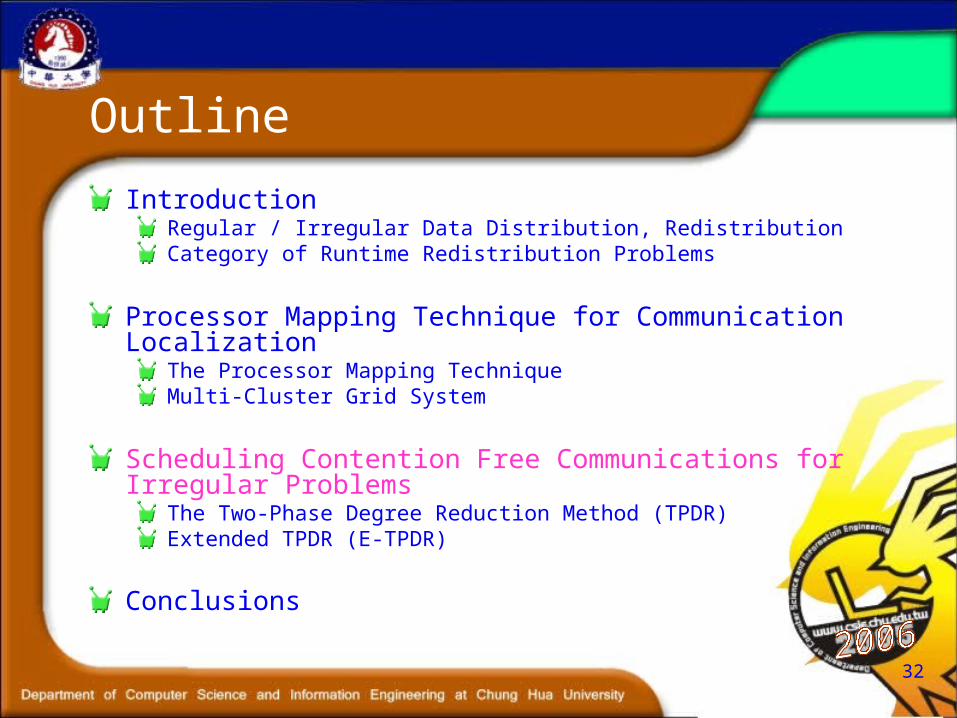
Outline
IntroductionRegular / Irregular Data Distribution, RedistributionCategory of Runtime Redistribution Problems
Processor Mapping Technique for Communication Localization
The Processor Mapping TechniqueMulti-Cluster Grid System
Scheduling Contention Free Communications for Irregular Problems
The Two-Phase Degree Reduction Method (TPDR)Extended TPDR (E-TPDR)
Conclusions

33
Example of GEN_BLOCK distributions
Enhance load balancing on heterogeneous environment
Scheduling Irregular Redistributions
Data distribution for algorithm P
7 16 11 10 7 49
Data distribution for algorithm Q
15 16 10 16 15 28
Application
……
Algorithm P
Algorithm Q
34
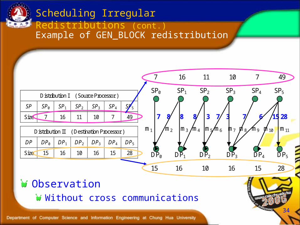
Example of GEN_BLOCK redistribution
Scheduling Irregular Redistributions (cont.)
Distribution I ( Source Processor )
SP SP0 SP1 SP2 SP3 SP4 SP5
Size 7 16 11 10 7 49
Distribution II ( Destination Processor )
DP DP0 DP1 DP2 DP3 DP4 DP5
Size 15 16 10 16 15 28
m11 m10 m9 m8 m7 m6 m5 m4 m3 m2 m1
7 8 8 8 3 7 3 7 6 15 28
15 16 10 16 15 28
m6 DP0 DP1 DP2 DP3 DP4 DP5
SP0 SP1 SP2 SP3 SP4 SP5
7 16 11 10 7 49
ObservationWithout cross communications

35
Convex Bipartite Graph
Scheduling Irregular Redistributions (cont.)
SP2
TP1 TP2 TP3
SP3SP1
:NodeData communication
:
36
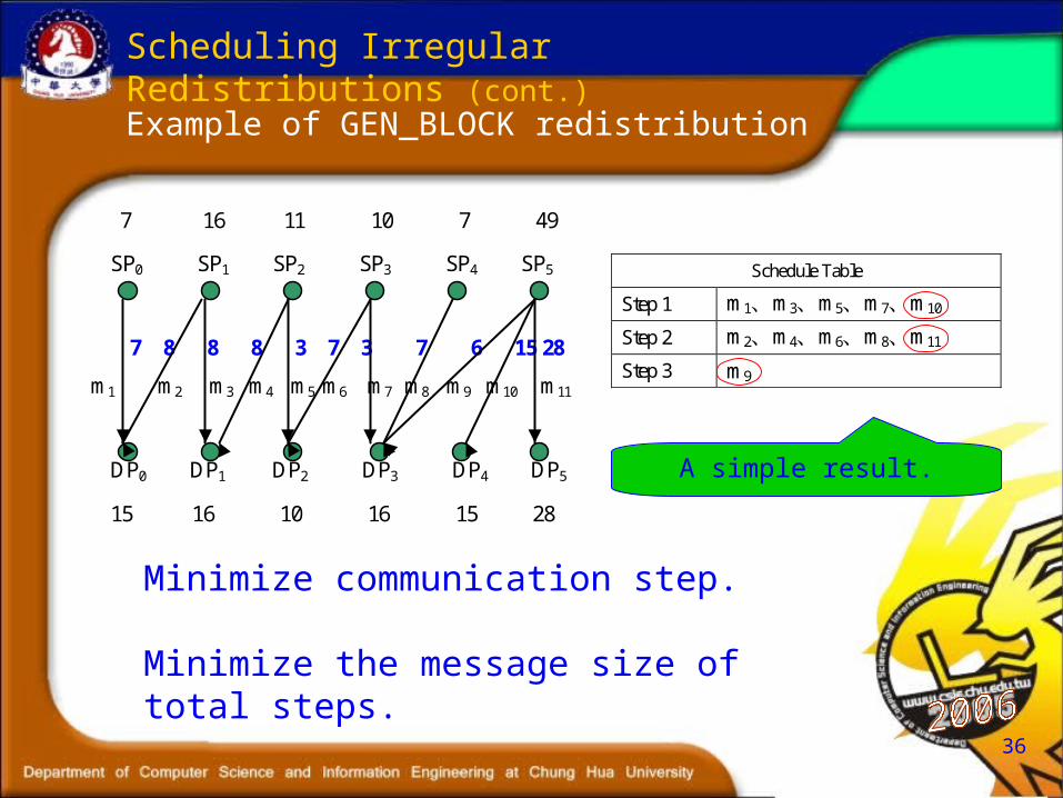
Example of GEN_BLOCK redistribution
Scheduling Irregular Redistributions (cont.)
m11 m10 m9 m8 m7 m6 m5 m4 m3 m2 m1
7 8 8 8 3 7 3 7 6 15 28
15 16 10 16 15 28
m6 DP0 DP1 DP2 DP3 DP4 DP5
SP0 SP1 SP2 SP3 SP4 SP5
7 16 11 10 7 49
Schedule Table
Step 1 m1、m3、m5、m7、m10
Step 2 m2、m4、m6、m8、m11
Step 3 m9
A simple result.
Minimize communication step.
Minimize the message size of total steps.
37
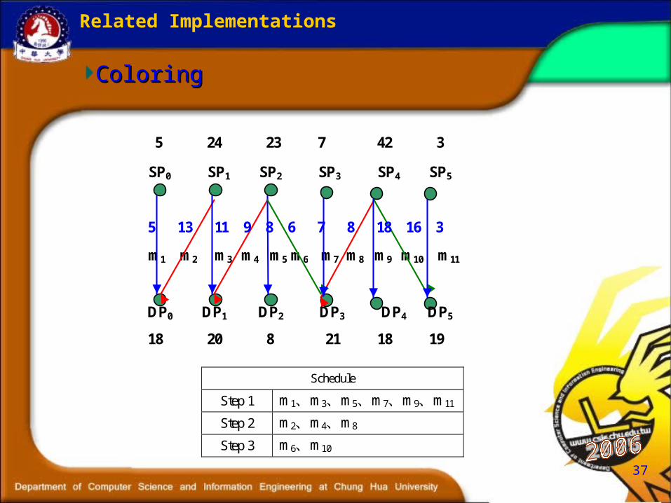
Related Implementations
ColoringColoring
m11 m10 m9 m8 m7 m6 m5 m4 m3 m2 m1
18 20 8 21 18 19
SP0 SP1 SP2 SP3 SP4 SP5
5 24 23 7 42 3
DP0 DP1 DP2 DP3 DP4 DP5
5 13 11 9 8 6 7 8 18 16 3
Schedule
Step 1 m1、m3、m5、m7、m9、m11
Step 2 m2、m4、m8
Step 3 m6、m10

38
Related Implementations
LISTLIST
Schedule
Step 1 m2、m4、m7、m9、m11
Step 2 m1、m3、m5、m10
Step 3 m8
Step 4 m6
m11 m10 m9 m8 m7 m6 m5 m4 m3 m2 m1
18 20 8 21 18 19
SP0 SP1 SP2 SP3 SP4 SP5
5 24 23 7 42 3
DP0 DP1 DP2 DP3 DP4 DP5
5 13 11 9 8 6 7 8 18 16 3

39
Related Implementations
DC1 & DC2DC1 & DC2
m11 m10 m9 m8 m7 m6 m5 m4 m3 m2 m1
18 20 8 21 18 19
SP0 SP1 SP2 SP3 SP4 SP5
5 24 23 7 42 3
DP0 DP1 DP2 DP3 DP4 DP5
5 13 11 9 8 6 7 8 18 16 3
1 2 3 4 5 6 7 8 9 10 11
Separating NMS
Schedule 1
Step 1 m2
Step 2 m3
Step 3 m1
Schedule 2
Step 1 m2
Step 2 m1、m3
(b)DC2(a)DC1
Schedule
Step 1 m2、m4、m7、m9、m11
Step 2 m3、m6、m10
Step 3 m1、m5、m8
Schedule
Step 1 m2、m4、m7、m9、m11
Step 2 m6、m10
Step 3 m1、m3、m5、m8

40
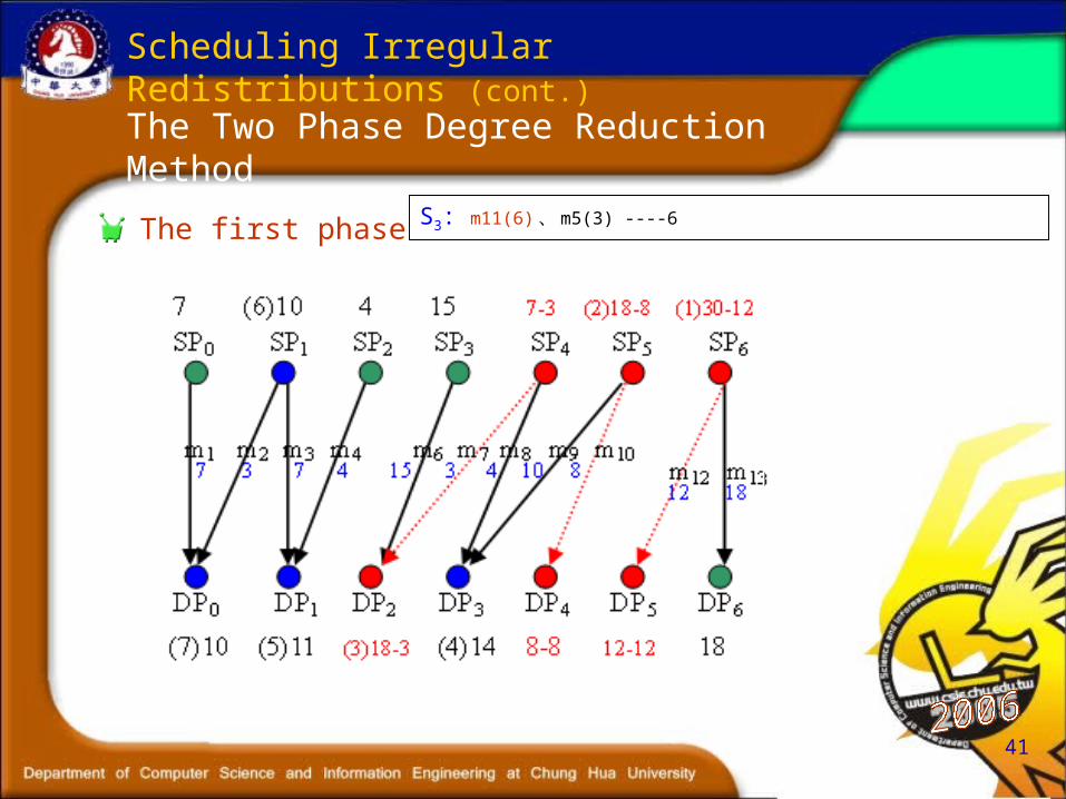
The Two Phase Degree Reduction Method
Scheduling Irregular Redistributions (cont.)
The First Phase (for nodes with degree >2)Reduces degree of the maximum degree nodes by one in each reduction iteration.
The Second Phase (for nodes with degree = 1 and 2)
Schedules messages between nodes that with degree 1 and 2 using an adjustable coloring mechanism.
41
The first phase
Scheduling Irregular Redistributions (cont.)
The Two Phase Degree Reduction Method
S3: m11(6) 、 m5(3) ----6
42
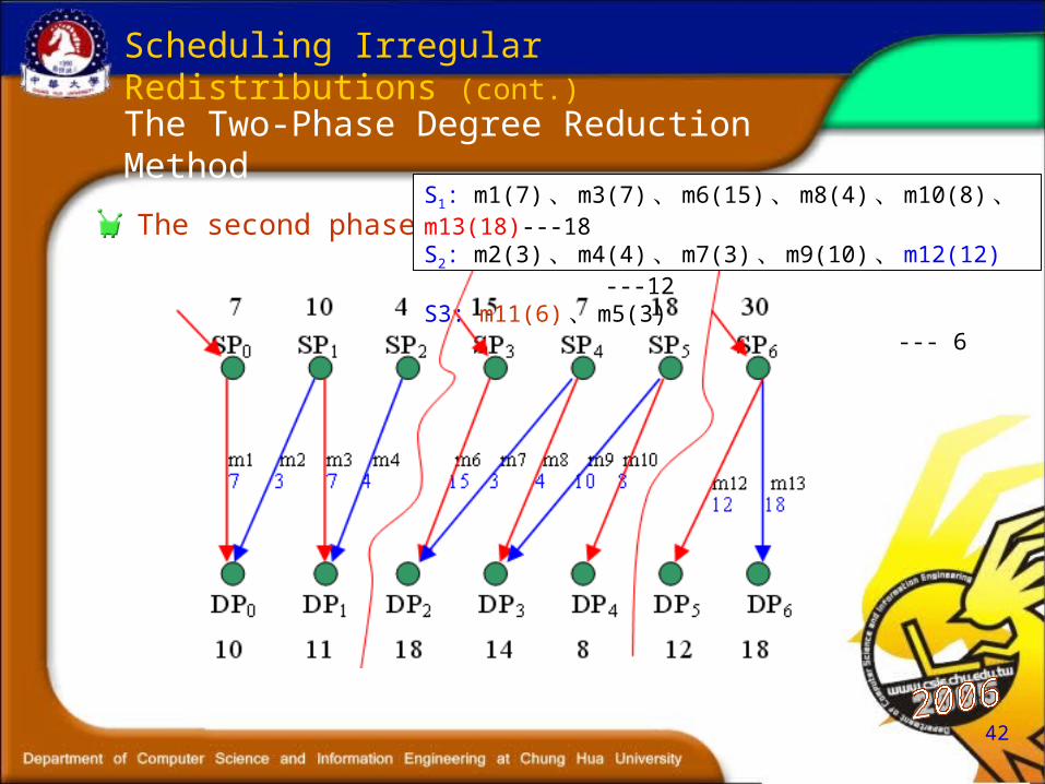
The second phase
Scheduling Irregular Redistributions (cont.)
The Two-Phase Degree Reduction Method
S1: m1(7) 、 m3(7) 、 m6(15) 、 m8(4) 、 m10(8) 、 m13(18)---18S2: m2(3) 、 m4(4) 、 m7(3) 、 m9(10) 、 m12(12) ---12S3: m11(6) 、 m5(3) --- 6

43
Scheduling Irregular Redistributions (cont.)
Extend TPDR
S1: m1(7) 、 m3(7) 、 m6(15) 、 m9(10) 、 m13(18) ---18S2: m4(4) 、 m7(3) 、 m10(8) 、 m12(12) ---12S3: m11(6) 、 m5(3) 、 m2(3) m2(3) 、 m8(4)m8(4) ----6
S1: m1(7) 、 m3(7) 、 m6(15) 、 m8(4) 、 m10(8) 、 m13(18)---18S2: m2(3) 、 m4(4) 、 m7(3) 、 m9(10) 、 m12(12) ---12S3: m11(6) 、 m5(3) --- 6
TPDRTPDR
E-TPDRE-TPDR

44
Performance Evaluation
Simulation of TPDR and E-TPDR algorithms on uneven
cases.

45
Performance Evaluation (cont.)
Simulation A is carried out to examine the performance
of TPDR and E-TPDR algorithms on uneven cases.

46
Performance Evaluation (cont.)
Simulation B is carried out to examine the performance
of TPDR and E-TPDR algorithms on even cases.
47
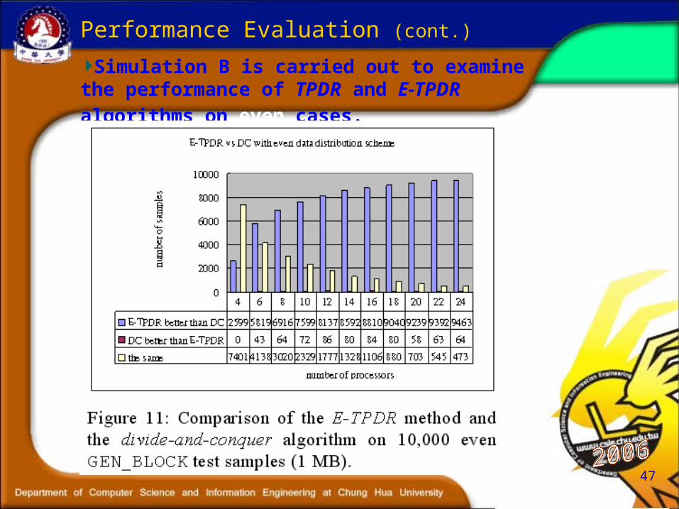
Performance Evaluation (cont.)
Simulation B is carried out to examine the performance
of TPDR and E-TPDR algorithms on even cases.

48
Summary
TPDR & E-TPDR for Scheduling irregular GEN_BLOCK redistributions
Contention freeOptimal Number of Communication StepsOutperforms the D&C algorithmTPDR(uneven) performs better than TPDR(even)

49
1000 test cases
Performance Evaluation (cont.)
Processor:8 DR LIST DC1 DC2 Color Combined
DR better
equal
worse
207
535
258
856
99
45
669
312
19
957
37
6
67.225%
24.575%
8.2%
LIST better
equal
worse
258
535
207
874
101
25
738
165
97
975
4
21
71.125%
20.125%
8.75%
DC1 better
equal
worse
45
99
856
25
101
874
243
92
665
755
101
144
26.7%
9.825%
63.475%
DC2 better
equal
worse
19
312
669
97
165
738
665
92
243
901
39
60
42.05%
15.2%
42.75%
Color better
equal
worse
6
37
957
21
4
975
144
101
755
60
39
901
5.775%
4.525%
89.7%
Processor:16 DR LIST DC1 DC2 Coloring Combined
DR better
equal
worse
331
379
290
985
5
10
931
58
11
998
2
0
81.125%
11.1%
7.775%
LIST better
equal
worse
290
379
331
989
4
7
921
25
54
998
0
2
79.95%
10.2%
9.85%
DC1 better
equal
worse
10
5
985
7
4
989
179
11
810
774
42
184
24.25%
1.55%
74.2%
DC2 better
equal
worse
11
58
931
54
25
921
810
11
179
948
7
45
45.575%
2.525%
51.9%
Coloring better
equal
worse
0
2
998
2
0
998
184
42
774
45
7
948
5.775%
1.275%
92.95%
Processor:32 DR LIST DC1 DC2 Coloring Combined
DR better
equal
worse
400
278
322
999
0
1
994
4
2
1000
0
0
84.825%
7.05%
8.125%
LIST better
equal
worse
322
278
400
1000
0
0
994
1
5
1000
0
0
82.9%
6.975%
10.125%
DC1 better
equal
worse
1
0
999
0
0
1000
95
6
899
799
23
178
22.375%
0.725%
76.9%
DC2 better
equal
worse
2
4
994
5
1
994
899
6
95
969
1
30
46.875%
0.3%
52.825%
Coloring better
equal
worse
0
0
1000
0
0
1000
178
23
799
30
1
969
5.2%
0.6%
94.2%
Processor:64 DR LIST DC1 DC2 Coloring Combined
DR better
equal
worse
416
221
363
1000
0
0
999
0
1
1000
0
0
85.38%
5.525%
9.1%
LIST better
equal
worse
363
221
416
1000
0
0
1000
0
0
1000
0
0
84.08%
5.525%
10.4%
DC1 better
equal
worse
0
0
1000
0
0
1000
44
0
956
783
22
195
20.68%
0.55%
78.78%
DC2 better
equal
worse
1
0
999
0
0
1000
956
0
44
986
4
10
48.58%
0.1%
51.33%
Coloring better
equal
worse
0
0
1000
0
0
1000
195
22
783
10
4
986
5.125%
0.65%
94.23%
Processor:128 DR LIST DC1 DC2 Coloring Combined
DR better
equal
worse
473
204
323
1000
0
0
1000
0
0
1000
0
0
86.825%
5.1%
8.075%
LIST better
equal
worse
323
204
473
1000
0
0
1000
0
0
1000
0
0
83.075%
5.1%
11.825%
DC1 better
equal
worse
0
0
1000
0
0
1000
14
1
985
776
20
204
19.75%
0.525%
79.725%
DC2 better
equal
worse
0
0
1000
0
0
1000
985
1
14
998
0
2
49.575%
0.025%
50.4%
Coloring better
equal
worse
0
0
1000
0
0
100
204
20
776
2
0
998
5.15%
0.5%
94.35%

50
Average
8 16 32 64 1280
10
20
30
40
50
60
70
80
90
100Combined (Date szie = 10000)
Number of processors
Per
cent
( %
)
DRLISTDC1DC2COLOR
Performance Evaluation (cont.)

51
Conclusions
Runtime Data Redistribution is usually used to enhance algorithm performance in data parallel applications
Processor Mapping technique minimizes data transmission cost and achieves better communication localization on multi-cluster grid systems
TPDR & E-TPDR for Scheduling irregular GEN_BLOCK redistributions
Contention freeGood performance
Future WorksIncorporate localization techniques on Data Grid with considering Heterogeneous external communication overheadsIncorporate the ratio between local memory access & remote message passing (on different architecture) into E-TPDR scheduling policy…

52
Thank you
53
Our Implementation of Communication Scheduling
E-TPDRE-TPDR
m11 m10 m9 m8 m7 m6 m5 m4 m3 m2 m1
18 20 8 21 18 19
SP0 SP1 SP2 SP3 SP4 SP5
5 24 23-8 7 42-8 3
DP0 DP1 DP2 DP3 DP4 DP5
5 13 11 9 8 6 7 8 18 16 3
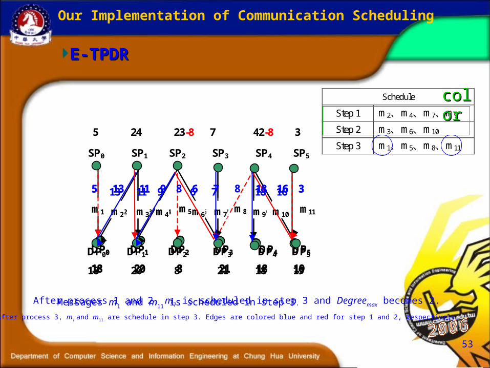
After process 1 and 2, m7 is scheduled in step 3 and Degreemax becomes 2.
m11 m10 m9 m7 m6 m4 m3 m2 m1
18 20 8 21 18 19
SP0 SP1 SP2 SP3 SP4 SP5
5 24 23-8 7 42-8 3
DP0 DP1 DP2 DP3 DP4 DP5
5 13 11 9 6 7 18 16 3
Messages m1 and m11 is scheduled in step 3.
m10 m9 m7 m6 m4 m3 m2
18 20 8 21 18 19
SP0 SP1 SP2 SP3 SP4 SP5
5 24 23-8 7 42-8 3
DP0 DP1 DP2 DP3 DP4 DP5
13 11 9 6 7 18 16
After process 3, m1 and m11 are schedule in step 3. Edges are colored blue and red for step 1 and 2, respectively.
Schedule
Step 1 m2、m4、m7、m9
Step 2 m3、m6、m10
Step 3 m1、m5、m8、m11
colorcolor