1 identiﬁcation of parametric underspread linear...

arX

iv:1

008.

0851

v2 [

cs.IT

] 7

Dec

201

01

Identification of Parametric Underspread Linear

Systems and Super-Resolution RadarWaheed U. Bajwa,Member, IEEE, Kfir Gedalyahu, and Yonina C. Eldar,Senior Member, IEEE

Abstract

Identification of time-varying linear systems, which introduce both time-shifts (delays) and frequency-

shifts (Doppler-shifts), is a central task in many engineering applications. This paper studies the problem

of identification of underspread linear systems (ULSs), whose responses lie within a unit-area region in the

delay–Doppler space, by probing them with a known input signal. It is shown that sufficiently-underspread

parametric linear systems, described by a finite set of delays and Doppler-shifts, are identifiable from a

single observation as long as the time–bandwidth product ofthe input signal is proportional to the square

of the total number of delay–Doppler pairs in the system. In addition, an algorithm is developed that

enables identification of parametric ULSs from an input train of pulses in polynomial time by exploiting

recent results on sub-Nyquist sampling for time delay estimation and classical results on recovery of

frequencies from a sum of complex exponentials. Finally, application of these results to super-resolution

target detection using radar is discussed. Specifically, itis shown that the proposed procedure allows

to distinguish between multiple targets with very close proximity in the delay–Doppler space, resulting

in a resolution that substantially exceeds that of standardmatched-filtering based techniques without

introducing leakage effects inherent in recently proposedcompressed sensing-based radar methods.

Index Terms

Compressed sensing, Delay–Doppler estimation, rotational invariance techniques, super-resolution

radar, system identification, time-varying linear systems

W.U. Bajwa is with the Department of Electrical and ComputerEngineering, Duke University, Durham, NC 27707

USA (Email: [email protected]). K. Gedalyahu and Y.C. Eldar are with the Department of Electrical Engineering,

Technion—Israel Institute of Technology, Haifa 32000, Israel (Phone: +972-4-8293256, Fax: +972-4-8295757, E-mails:

kfirge@techunix,[email protected]. Y.C. Eldar is currently also a Visiting Professor at Stanford

University, Stanford, CA 94305 USA.

December 8, 2010 DRAFT

http://arxiv.org/abs/1008.0851v2

2

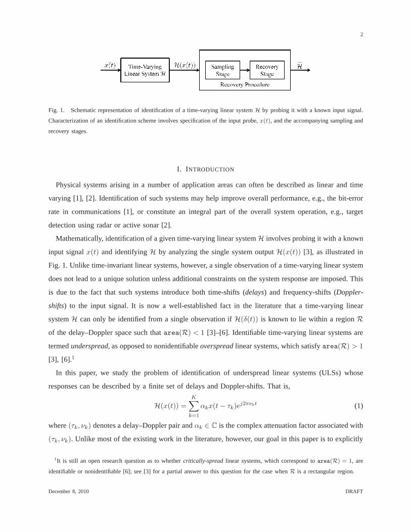
Fig. 1. Schematic representation of identification of a time-varying linear systemH by probing it with a known input signal.

Characterization of an identification scheme involves specification of the input probe,x(t), and the accompanying sampling and

recovery stages.

I. INTRODUCTION

Physical systems arising in a number of application areas can often be described as linear and time

varying [1], [2]. Identification of such systems may help improve overall performance, e.g., the bit-error

rate in communications [1], or constitute an integral part of the overall system operation, e.g., target

detection using radar or active sonar [2].

Mathematically, identification of a given time-varying linear systemH involves probing it with a known

input signalx(t) and identifyingH by analyzing the single system outputH(x(t)) [3], as illustrated in

Fig. 1. Unlike time-invariant linear systems, however, a single observation of a time-varying linear system

does not lead to a unique solution unless additional constraints on the system response are imposed. This

is due to the fact that such systems introduce both time-shifts (delays) and frequency-shifts (Doppler-

shifts) to the input signal. It is now a well-established fact in theliterature that a time-varying linear

systemH can only be identified from a single observation ifH(δ(t)) is known to lie within a regionRof the delay–Doppler space such thatarea(R) < 1 [3]–[6]. Identifiable time-varying linear systems are

termedunderspread, as opposed to nonidentifiableoverspreadlinear systems, which satisfyarea(R) > 1

[3], [6].1

In this paper, we study the problem of identification of underspread linear systems (ULSs) whose

responses can be described by a finite set of delays and Doppler-shifts. That is,

H(x(t)) =

K∑

k=1

αkx(t− τk)ej2πνkt (1)

where(τk, νk) denotes a delay–Doppler pair andαk ∈ C is the complex attenuation factor associated with

(τk, νk). Unlike most of the existing work in the literature, however, our goal in this paper is to explicitly

1It is still an open research question as to whethercritically-spread linear systems, which correspond toarea(R) = 1, are

identifiable or nonidentifiable [6]; see [3] for a partial answer to this question for the case whenR is a rectangular region.


3

characterize conditions on the bandwidth and temporal support of the input signal that ensure identification

of such ULSs from single observations. The importance of this goal can be best put into perspective

by realizing that ULSs of the form (1) tend to arise frequently in many applications. Consider, for

example, a single-antenna transmitter communicating wirelessly with a single-antenna receiver in a mobile

environment. Over a small-enough time interval, the channel between the transmitter and receiver is of the

form (1) with each triplet(τk, νk, αk) corresponding to a distinct physical path between the transmitter

and receiver [7]. Identification ofH can enable one to establish a relatively error-free communication link

between the transmitter and receiver. But wireless systemsalso need to identify channels using signals

that have as smalltime–bandwidth productas possible so that they can allocate the rest of the temporal

degrees of freedom to communicating data [7], [8].

Similarly, in the case of target detection using radar or active sonar, the (noiseless, clutter-free) received

signal is of the form (1) with each triplet(τk, νk, αk) corresponding to an echo of the transmitted signal

from a distinct target in the delay–Doppler space [2]. Identification of H in this case enables one to

accurately obtain the radial position and velocity of the targets. Radar systems also strive to operate with

signals (waveforms) that have as small temporal support andbandwidth as possible. This is because the

temporal support of the radar waveform is directly tied to the time it takes to identify all the targets while

the bandwidth of the waveform—among other technical considerations—is tied to the sampling rate of

the radar receiver [2].

Given the ubiquity of time-varying linear systems in engineering applications, there exists considerable

amount of existing literature that studies identification of such systems in an abstract setting. Kailath was

the first to recognize that the identifiability of a time-varying linear systemH from a single observation

is directly tied to the area of the regionR that containsH(δ(t)) [4]. Kailath’s seminal work in [4] laid

the foundations for the future works of Bello [5], Kozek and Pfander [3], and Pfander and Walnut [6],

which establish the nonidentifiability of overspread linear systems and provide constructive proofs for

the identifiability of arbitrary ULSs. However, none of these results shed any light on the bandwidth and

temporal support of the input signal needed to ensure identification of ULSs of the form (1). On the

contrary, the constructive proofs provided in [3]–[6] require use of input signals with infinite bandwidth

and temporal support.

In contrast, to the best of our knowledge, this is the first paper to develop a theory for identification

of ULSs of the form (1), henceforth referred to asparametricULSs, that parallels that of [3]–[6] for

identification of arbitrary ULSs. One of the main contributions of this paper is that we establish using a

constructive proof that sufficiently-underspread parametric linear systems are identifiable as long as the


4

time–bandwidth product of the input signal is proportionalto the square of the total number of delay–

Doppler pairs in the system. Equally importantly, as part ofour constructive proof, we concretely specify

the nature of the input signal (a finite train of pulses) and the structure of a corresponding polynomial-

time (in the number of delay–Doppler pairs) recovery procedure that enable identification of parametric

ULSs. These ideas are also immediately applicable to super-resolution target detection using radar and

we show in the latter part of the paper that our approach indeed results in a resolution that substantially

exceeds that of standard matched-filtering based techniques without introducing leakage effects inherent

in recently proposed compressed sensing-based radar methods [9].

The key developments in the paper leverage recent results onsub-Nyquist sampling for time-delay

estimation [10] and classical results on direction-of-arrival (DOA) estimation [11]–[14]. Unlike the

traditional DOA estimation literature, however, we do not assume that the system output is observed

by an array of antennas. Additionally, in contrast to [10], our goal here is not a reduction in the sampling

rate; rather, we are interested in characterizing the minimum temporal degrees of freedom of the input

signal needed to ensure identification of a parametric ULSH. The connection to sub-Nyquist sampling

can be understood by noting that the sub-Nyquist sampling results of [10] enable recovery of the delays

associated withH using a small-bandwidth input signal. Further, the “train-of-pulses” nature of the input

signal combined with results on recovery of frequencies from a sum of complex exponentials [14] allow

recovery of the Doppler-shifts and attenuation factors using an input signal of small temporal support.

Several works in the past have considered identification of specialized versions of parametric ULSs.

Specifically, [9], [15]–[18] treat parametric ULSs whose delays and Doppler-shifts lie on a quantized

grid in the delay–Doppler space. On the other hand, [19] considers the case in which there are no more

than two Doppler-shifts associated with the same delay. Theproposed recovery procedures in [19] also

have exponential complexity, since they require exhaustive searches in aK-dimensional space, and stable

initializations of these procedures stipulate that the system output be observed by anM -element antenna

array withM ' K.

While the insights of [9], [15]–[18] can be extended to arbitrary parametric ULSs by taking infinitesimally-

fine quantization of the delay–Doppler space, this will require input signals with infinite bandwidth and

temporal support. In contrast, our ability to avoid quantization of the delay–Doppler space is due to

the fact that we treat the system-identification problem directly in the analog domain. This follows the

philosophy in much of the recent work in analog compressed sensing, termed Xampling, which provides

a framework for incorporating and exploiting structure in analog signals without the need for quantization

[20]–[25]. This is in particular the key enabling factor that helps us avoid the catastrophic implications


5

of the leakage effects in the context of radar target detection.

Before concluding this discussion, we note that responses of arbitrary ULSs can always be represented

as (1) under the limitK → ∞. Therefore, the main result of this paper can also be construed as an

alternate constructive proof of the identifiability of sufficiently-underspread linear systems. Nevertheless,

just like [3]–[6], this interpretation of the presented results again seem to suggest that identification of

arbitrary ULSs requires use of input signals with infinite bandwidth and temporal support.

The rest of this paper is organized as follows. In Section II,we formalize the problem of identification

of parametric ULSs along with the accompanying assumptions. In Section III, we propose a polynomial-

time recovery procedure used for the identification of parametric ULSs, while Section IV specifies the

conditions on the input signal needed to guarantee unique identification using the proposed procedure.

We compare the results of this paper to some of the related literature on identification of parametric

ULSs in Section V and discuss an application of our results tosuper-resolution target detection using

radar in Section VI. Finally, we present results of some numerical experiments in Section VII.

We make use of the following notational convention throughout this paper. Vectors and matrices are

denoted by bold-faced lowercase and bold-faced uppercase letters, respectively. Thenth element of a

vectora is written asan, and the(i, j)th element of a matrixA is denoted byAij . Superscripts(·)∗,(·)T and(·)H represent conjugation, transposition, and conjugate transposition, respectively. In addition,

the Fourier transform of a continuous-time signalx (t) ∈ L2(C) is defined byX (ω) =∫∞

−∞x (t) e−jωtdt,

while 〈x (t) , y (t)〉 =∫∞

−∞x (t) y∗(t)dt denotes the inner product between two continuous-time signals

in L2(C). Similarly, the discrete-time Fourier transform of a sequence a [n] ∈ ℓ2(C) is defined by

A(ejωT

)=

∑n∈Z a [n] e

−jωnT and is periodic inω with period2π/T . Finally, we useA† to write the

Moore–Penrose pseudoinverse of a matrixA.

II. PROBLEM FORMULATION AND MAIN RESULTS

In this section, we formalize the problem of identification of a parametric ULSH whose response is

described by a total ofK arbitrary delay–Doppler-shifts of the input signal. The task of identification of

H essentially requires specifying two distinct but highly intertwined steps. First, we need to specify the

conditions on the bandwidth and temporal support of the input signalx(t) that ensure identification ofHfrom a single observation. Second, we need to provide a polynomial-time recovery procedure that takes

as inputH(x(t)) and provides an estimateH of the system response by exploiting the properties ofx(t)

specified in the first step. We begin by detailing our system model and the accompanying assumptions.

In (1), some of the delays,τk, might be repeated. ExpressingH in terms ofKτ ≤ K distinct delays


6

in this case leads to

H(x(t)) =

Kτ∑

i=1

Kν,i∑

j=1

αijx(t− τi)ej2πνijt (2)

whereνij denotes thejth Doppler-shift associated with theith distinct delayτi, αij ∈ C denotes the

attenuation factor associated with the delay–Doppler pair(τi, νij), andK =∑Kτ

i=1Kν,i. We choose to

expressH(x(t)) as in (2) so as to facilitate the forthcoming analysis. Throughout the rest of the paper,

we useτ = τi, i = 1, . . . ,Kτ to denote the set ofKτ distinct delays associated withH. The first

main assumption that we make concerns the footprint ofH in the delay–Doppler space:

[A1] The responseH(δ(t)) of H lies within a rectangular region of the delay–Doppler space; in other

words, (τi, νij) ∈ [0, τmax] × [−νmax/2, νmax/2]. This is indeed the case in many engineering

applications (see, e.g., [1], [2]). The parametersτmax andνmax are termed in the parlance of linear

systems as thedelay spreadand theDoppler spreadof the system, respectively.

Next, we useT andW to denote the temporal support and the two-sided bandwidth of the known

input signalx(t) used to probeH, respectively. We propose using input signals that correspond to a finite

train of pulses:

x(t) =

N−1∑

n=0

xng(t− nT ), 0 ≤ t ≤ T (3)

whereg(t) is a prototype pulse of bandwidthW that is (essentially) temporally supported on[0, T ] and

is assumed to have unit energy(∫|g(t)|2dt = 1), and xn ∈ C is anN -length probing sequence.

The parameterN is proportional to the time–bandwidth product ofx(t), which roughly defines the

number of temporal degrees of freedom available for estimating H [8]: N = T /T ∝ T W.2 The final

two assumptions that we make concern the relationship between the delay spreadτmax and the Doppler

spreadνmax of H, and the temporal supportT and bandwidthW of g(t):

[A2] The delay spread ofH is strictly smaller than the temporal support ofg(t): τmax < T , and

[A3] The Doppler spread ofH is much smaller than the bandwidth ofg(t): νmax ≪ W.

Note that, sinceW ∝ 1/T , [A3] equivalently imposes thatνmaxT ≪ 1. This assumption states that

the temporal scale of variations inH is large relative to the temporal scale of variations inx(t). It is

worth pointing out that linear systems that are sufficientlyunderspread in the sense thatτmaxνmax ≪ 1

can always be made to satisfy[A2] and [A3] for any given budget of the time–bandwidth product.

2Recall that the temporal support and the bandwidth of an arbitrary pulseg(t) are related to each other asW ∝ 1/T .


7

Remark1. In order to elaborate on the validity of[A2] and[A3], note that there exist many communication

applications where underlying linear systems tend to be highly underspread [1,§ 14.2]. Similarly, [A2]

and [A3] in the context of radar target detection simply mean that thetargets are not too far away from

the radar and that their velocities are not too high. Consider, for example, anL-band radar (operating

frequency of1.3 GHz) that transmits a pulseg(t) of bandwidthW = 10 MHz after everyT = 50 µs.

Then both[A2] and[A3] are satisfied when the distance between the radar and any target is at most7.5

km (τmax ≈ 50 µs) and the radial velocity of any target is at most185 km/h (νmax ≈ 445 Hz) [2].

The following theorem summarizes our key result concerningidentification of parametric ULSs.

Theorem 1 (Identification of Parametric Underspread Linear Systems). Suppose thatH is a parametric

ULS that is completely described by a total ofK =∑Kτ

i=1Kν,i triplets (τi, νij , αij). Then, irrespective

of the distribution of(τi, νij) within the delay–Doppler space,H can be identified in polynomial-time

from a single observationH(x(t)) as long as it satisfies[A1]–[A3], the probing sequencexn remains

bounded away from zero in the sense that|xn| > 0 for everyn = 0, . . . , N − 1, and the time–bandwidth

product of the known input signalx(t) satisfies the condition

T W ≥ 8πKτKν,max (4)

whereKν,max = maxiKν,i is the maximum number of Doppler-shifts associated with anyone of the

distinct delays. In addition, the time–bandwidth product of x(t) is guaranteed to satisfy(4) as long as

T W ≥ 2π(K + 1)2.

The rest of this paper is devoted to providing a proof of Theorem 1. In terms of a general roadmap for the

proof, we first exploit the sub-Nyquist sampling results of [10] to argue thatx(t) with small bandwidth

suffices to recover the delays associated withH. We then exploit the “train-of-pulses” structure ofx(t) and

classical results on recovery of frequencies from a sum of complex exponentials [14] to argue thatx(t)

with small temporal support suffices to recover the Doppler-shifts and attenuation factors associated with

H. The statement of Theorem 1 will then follow by a simple combination of the two claims concerning

the bandwidth and temporal support ofx(t). We will make use of (2) and (3) in the following to describe:

[1] The polynomial-time recovery procedure used for the identification ofH (cf. Section III), and

[2] The accompanying conditions onx(t) needed to guarantee identification ofH (cf. Section IV).


8

Fig. 2. Schematic representation of the polynomial-time recovery procedure for identification of parametric underspread linear

systems from single observations.

III. POLYNOMIAL -TIME IDENTIFICATION OF ULSS

In this section, we characterize the polynomial-time recovery procedure used for identification of

ULSs of the form (2). In order to facilitate understanding ofthe proposed algorithm, shown in Fig. 2,

we conceptually partition the method into two stages: sampling and recovery. The rest of this section is

devoted to describing these two steps in detail. Before proceeding further, however, it is instructive to

first make use of (2) and (3) and rewrite the output ofH as

H(x(t)) =

Kτ∑

i=1

Kν,i∑

j=1

N−1∑

n=0

αijxnej2πνijtg(t− τi − nT )

(a)≈

Kτ∑

i=1

Kν,i∑

j=1

N−1∑

n=0

αijxnej2πνijnT g(t− τi − nT )

=

Kτ∑

i=1

N−1∑

n=0

ai[n]g(t − τi − nT ) (5)

where (a) follows from the assumptionνmaxT ≪ 1, which implies thatej2πνijt ≈ ej2πνijnT for all

t ∈ [(n− 1)T, nT ), and the sequencesai[n], i = 1, . . . ,Kτ , are defined as

ai[n] =

Kν,i∑

j=1

αijxnej2πνijnT , n = 0, . . . , N − 1. (6)

A. The Sampling Stage

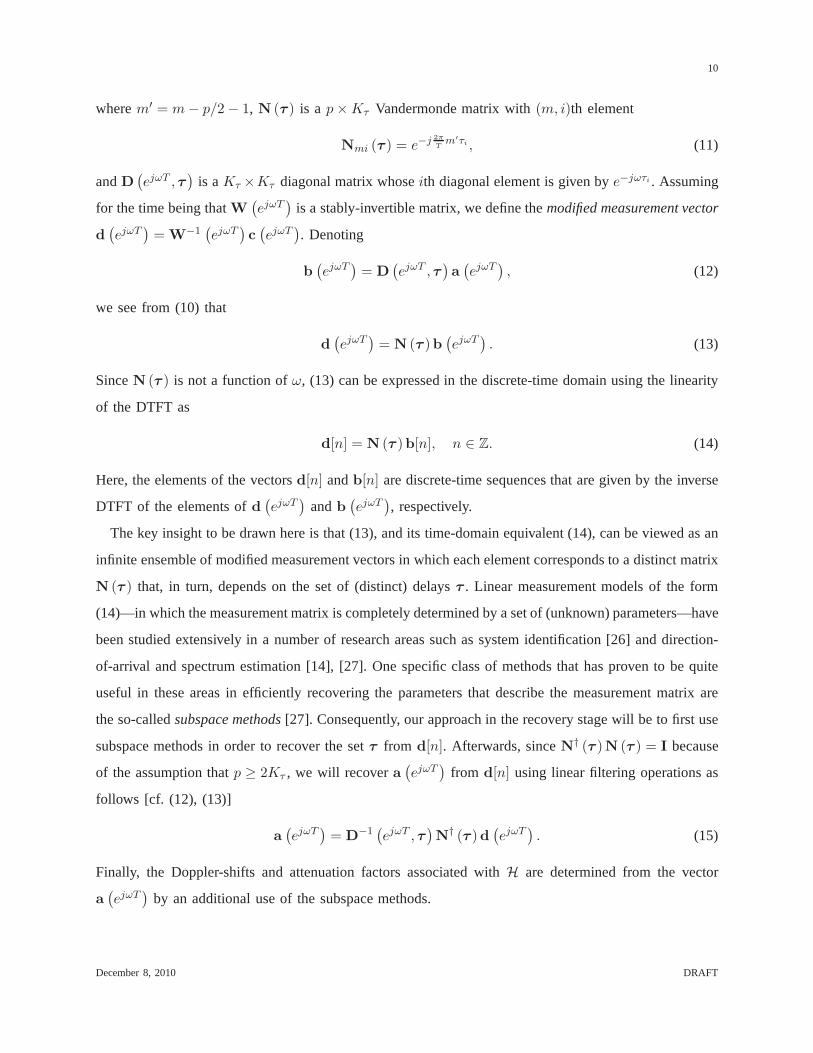
We leverage the ideas of [10] on time-delay estimation from sub-Nyquist samples to describe the

sampling stage of our recovery procedure. While the primaryobjective in [10] is time-delay estimation


9

from low-rate samples, the development here is carried out with an eye towards identification of parametric

ULSs regardless of the distribution of system parameters within the delay–Doppler space—the so-

calledsuper-resolution identification. In [10], a general multi-channel sub-Nyquist sampling scheme was

introduced for the purpose of recovering a set of unknown delays from signals of the form (5). Here,

we focus on one special case of that scheme, which consists ofa low-pass filter (LPF) followed by a

uniform sampler. This architecture may be preferable from an implementation viewpoint since it requires

only one sampling channel, thereby simplifying analog front-end of the sampling hardware. The LPF,

besides being required by the sampling stage, also serves asthe front-end of the system-identification

hardware and rejects noise and interference outside the working spectral band.

Our sampling stage first passes the system outputy(t) = H(x(t)) through a LPF whose impulse

response is given bys∗(−t) and then uniformly samples the LPF output at timest = nT/p

. We

assume that the frequency response,S∗(ω), of the LPF is contained in the spectral bandF , defined as

F =[−π

Tp,π

Tp], (7)

and is zero for frequenciesω /∈ F . Here, the parameterp is assumed to be even and satisfies the condition

p ≥ 2Kτ ; exact requirements onp to ensure identification ofH will be given in Section IV. In order to

relate the sampled output of the LPF with the multi-channel sampling formulation of [10], we definep

sampling (sub)sequencescℓ[n]

as

cℓ[n] = 〈y(t), s(t− nT − (ℓ− 1)T/p)〉 , ℓ = 1, . . . , p. (8)

These sequences correspond to periodically splitting the samples at the output of the LPF, which is

generated at a rate ofp/T , into p slower sequences at a rate of1/T each using a serial-to-parallel

converter; see Fig. 2 for a schematic representation of thissplitting.

Next, we define the vectorc(ejωT

)as thep-length vector whoseℓth element isCℓ

(ejωT

), which

denotes thediscrete-time Fourier transform(DTFT) of cℓ[n]. In a similar fashion, we definea(ejωT

)

as theKτ -length vector whoseith element is given byAi

(ejωT

), the DTFT ofai[n]. It can be shown

following the developments carried out in [10] that these two vectors are related to each other by

c(ejωT

)= W

(ejωT

)N (τ )D

(ejωT , τ

)a(ejωT

). (9)

Here,W(ejωT

)is a p× p matrix with (ℓ,m)th element

Wℓm

(ejωT

)= ejω(ℓ−1)T/p 1

TS∗

(ω +

2π

Tm′

)G

(ω +

2π

Tm′

)ej

2π

p(ℓ−1)m′

, (10)


10

wherem′ = m− p/2− 1, N (τ ) is a p×Kτ Vandermonde matrix with(m, i)th element

Nmi (τ ) = e−j 2π

Tm′τi , (11)

andD(ejωT , τ

)is aKτ ×Kτ diagonal matrix whoseith diagonal element is given bye−jωτi . Assuming

for the time being thatW(ejωT

)is a stably-invertible matrix, we define themodified measurement vector

d(ejωT

)= W

−1(ejωT

)c(ejωT

). Denoting

b(ejωT

)= D

(ejωT , τ

)a(ejωT

), (12)

we see from (10) that

d(ejωT

)= N (τ )b

(ejωT

). (13)

SinceN (τ ) is not a function ofω, (13) can be expressed in the discrete-time domain using thelinearity

of the DTFT as

d[n] = N (τ )b[n], n ∈ Z. (14)

Here, the elements of the vectorsd[n] andb[n] are discrete-time sequences that are given by the inverse

DTFT of the elements ofd(ejωT

)andb

(ejωT

), respectively.

The key insight to be drawn here is that (13), and its time-domain equivalent (14), can be viewed as an

infinite ensemble of modified measurement vectors in which each element corresponds to a distinct matrix

N (τ ) that, in turn, depends on the set of (distinct) delaysτ . Linear measurement models of the form

(14)—in which the measurement matrix is completely determined by a set of (unknown) parameters—have

been studied extensively in a number of research areas such as system identification [26] and direction-

of-arrival and spectrum estimation [14], [27]. One specificclass of methods that has proven to be quite

useful in these areas in efficiently recovering the parameters that describe the measurement matrix are

the so-calledsubspace methods[27]. Consequently, our approach in the recovery stage willbe to first use

subspace methods in order to recover the setτ from d[n]. Afterwards, sinceN† (τ )N (τ ) = I because

of the assumption thatp ≥ 2Kτ , we will recovera(ejωT

)from d[n] using linear filtering operations as

follows [cf. (12), (13)]

a(ejωT

)= D

−1(ejωT , τ

)N

† (τ )d(ejωT

). (15)

Finally, the Doppler-shifts and attenuation factors associated with H are determined from the vector

a(ejωT

)by an additional use of the subspace methods.


11

Before proceeding to the recovery stage, we justify the assumption thatW(ejωT

)can be stably

inverted. To this end, observe from (10) thatW(ejωT

)can be decomposed as

W(ejωT

)= Φ

(ejωT

)FHΨ

(ejωT

), (16)

whereΦ(ejωT

)is a p× p diagonal matrix withℓth diagonal element

Φℓℓ

(ejωT

)=

√p(−1)ℓ−1ejω(ℓ−1)T/p, (17)

F is a p-point discrete Fourier transform (DFT) matrix with(ℓ,m)th element equal to

Fℓm =1√pe−j 2π

p(ℓ−1)(m−1), (18)

andΨ(ejωT

)is a p× p diagonal matrix whosemth diagonal element is given by

Ψmm

(ejωT

)=

1

TS∗

(ω +

2π

T(m− p/2− 1)

)G

(ω +

2π

T(m− p/2− 1)

). (19)

It can now be easily seen from the decomposition in (16) that,in order for W(ejωT

)to be stably

invertible, each of the above three matrices has to be stablyinvertible. By construction, bothΦ(ejωT

)

andFH are stably invertible. The invertibility requirement on the diagonal matrixΨ(ejωT

)leads to the

following conditions on the pulseg(t) and the kernels∗(−t) of the LPF.

Condition 1. In order for Ψ(ejωT

)to be stably invertible, the continuous-time Fourier transform of

g (t) has to satisfy

a ≤ |G (ω)| ≤ b a.e.ω ∈ F (20)

for some positive constantsa > 0 and b <∞.

Condition 2. In order for Ψ(ejωT

)to be stably invertible, the continuous-time Fourier transform of the

LPF s∗ (−t) has to satisfy

c ≤ |S (ω)| ≤ d a.e.ω ∈ F (21)

for some positive constantsc > 0 and d <∞.

Condition 1 requires that the bandwidthW of the prototype pulseg(t) has to satisfy

W ≥ 2π

Tp. (22)

In Section IV, we will derive additional conditions on the parameterp and combine them with (22) to

obtain equivalent requirements on the time–bandwidth product of the input signalx(t) that will ensure

invertibility of the matrixW(ejωT

).


12

We conclude discussion of the sampling stage by pointing outthat the decomposition in (16) also

provides an efficient way to implement the digital-correction filter bankW−1(ejωT

). This is because

(16) implies that

W−1

(ejωT

)= Ψ

−1(ejωT

)FΦ

−1(ejωT

). (23)

Therefore the implementation ofW−1(ejωT

)can be done in three stages, where each stage corresponds

to one of the three matrices in (23). Specifically, define the set of digital filtersφℓ[n] andψℓ[n] as

φℓ[n] = IDTFTΦ

−1ℓℓ

(ejωT

)[n], 1 ≤ ℓ ≤ p (24)

and

ψℓ[n] = IDTFTΨ

−1ℓℓ

(ejωT

)[n], 1 ≤ ℓ ≤ p, (25)

where IDTFT denotes the inverse DTFT operation. The first correction stage involves filtering the

sequencescℓ[n] using the set of filtersφℓ[n]. Next, multiplication with the DFT matrixF can

be efficiently implemented by applying the fast Fourier transform (FFT) to the outputs of the filters in

the first stage. Finally, the third correction stage involves filtering the resulting sequences using the set

of filters ψℓ[n] to get the desired sequencesdℓ[n]. This last correction stage can be interpreted as an

equalization step that compensates for the non-flatness of the frequency responses of the prototype pulse

and the kernel of the LPF. A detailed schematic representation of the sampling stage, which is based on

the preceding interpretation ofW−1(ejωT

), is provided in Fig. 2.

B. The Recovery Stage

We conclude this section by describing in detail the recovery stage, which—as noted earlier—consists

of two steps. In the first step, we rely on subspace methods to recover the delaysτ from d[n] [cf. (14)].

In the second step, we make use of the recovered delays to obtain the Doppler-shifts and attenuation

factors associated with each of the delays.

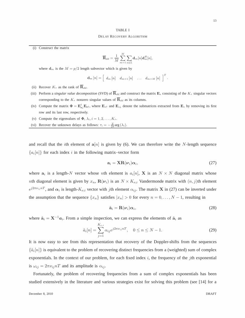
1) Recovery of the Delays:In order to recoverτ from d[n], we rely on the approach advocated in

[10] and make use of the well-known ESPRIT algorithm [28] together with an additional smoothing

stage [29]. The exact algorithm is given in Table I; we refer the reader to [10], [28] for details.

2) Recovery of the Doppler-Shifts and Attenuation Factors:Once the unknown delays are found, we

can recover the vectorsa[n] through the frequency relation (15). Next, define for each delay τi, the set

of corresponding Doppler-shifts

νi = νij , j = 1, . . . ,Kν,i (26)


13

TABLE I

DELAY RECOVERYALGORITHM

(i) Construct the matrix

Rdd =1

M

M∑

m=1

∑

n∈Z

dm[n]dH

m[n],

wheredm is theM = p/2 length subvector which is given by

dm [n] =[

dm [n] dm+1 [n] . . . dm+M [n]]T

.

(ii) RecoverKτ as the rank ofRdd.

(iii) Perform asingular value decomposition(SVD) of Rdd and construct the matrixEs consisting of theKτ singular vectors

corresponding to theKτ nonzero singular values ofRdd as its columns.

(iv) Compute the matrixΦ = E†s↓Es↑, whereEs↑ andEs↓ denote the submatrices extracted fromEs by removing its first

row and its last row, respectively.

(v) Compute the eigenvalues ofΦ, λi, i = 1, 2, . . . , Kτ .

(vi) Recover the unknown delays as follows:τi = − T

2πarg(λi).

and recall that theith element ofa[n] is given by (6). We can therefore write theN -length sequence

ai[n] for each indexi in the following matrix–vector form

ai = XR(ν i)αi, (27)

where ai is a length-N vector whosenth element isai[n], X is anN × N diagonal matrix whose

nth diagonal element is given byxn, R(ν i) is anN ×Kν,i Vandermonde matrix with(n, j)th element

ej2πνijnT , andαi is length-Kν,i vector withjth elementαij. The matrixX in (27) can be inverted under

the assumption that the sequencexn satisfies|xn| > 0 for everyn = 0, . . . , N − 1, resulting in

ai = R(νi)αi, (28)

whereai = X−1

ai. From a simple inspection, we can express the elements ofai as

ai[n] =

Kν,i∑

j=1

αijej2πνijnT , 0 ≤ n ≤ N − 1. (29)

It is now easy to see from this representation that recovery of the Doppler-shifts from the sequences

ai[n] is equivalent to the problem of recovering distinct frequencies from a (weighted) sum of complex

exponentials. In the context of our problem, for each fixed index i, the frequency of thejth exponential

is ωij = 2πνijnT and its amplitude isαij.

Fortunately, the problem of recovering frequencies from a sum of complex exponentials has been

studied extensively in the literature and various strategies exist for solving this problem (see [14] for a


14

review). One of these techniques that has gained interest recently, especially in the literature on finite rate

of innovation [30]–[33], is theannihilating-filter method. The annihilating-filter approach, in contrast to

some of the other techniques, allows the recovery of the frequencies associated with theith index even at

the critical value ofN = 2Kν,i. On the other hand, subspace methods such as ESPRIT [12], matrix-pencil

algorithm [13], and the Tufts and Kumaresan approach [11] are generally more robust to noise but also

require more samples than2Kν,i. Once the Doppler-shifts for each indexi have been recovered then,

sinceR†(νi)R(ν i) = I because of the requirement thatN ≥ 2Kν,i, the attenuation factorsαij are

determined as

αi = R†(νi)ai, i = 1, . . . ,Kτ . (30)

IV. SUFFICIENT CONDITIONS FOR IDENTIFICATION

Our focus in Section III was on developing a recovery algorithm for the identification of ULSs.

We now turn to specify conditions that guarantee that the proposed procedure recovers the set of triplets(τi, νij, αij)

that describe the parametric ULSH. We present these requirements in terms of equivalent

conditions on the time–bandwidth productT W of the input signalx(t). This is a natural way to describe

the performance of system identification schemes sinceT W roughly defines the number of temporal

degrees of freedom available for estimatingH [8].

To begin with, recall that the recovery stage involves first determining the unknown delaysτ from the

set of equations given by (14) (cf. Section III-B). Therefore, to ensure that our algorithm successfully

returns the parameters ofH, we first need to provide conditions that guarantee a unique solution to (14).

To facilitate the forthcoming analysis, we letd [Λ] = d [n] , n ∈ Z andb [Λ] = b [n] , n ∈ Z denote

the set of all vectorsd [n] andb [n], respectively. Using this notation, we can rewrite (14) as

d [Λ] = N (τ )b [Λ] . (31)

We now leverage the analysis carried out in [10] to provide sufficient conditions for a unique solution

to (31); see [10] for a formal proof.

Proposition 1. If(τ , b [Λ] 6= 0

)solves(31) and if

p > 2Kτ − dim(span

(b [Λ]

))(32)

then(τ , b [Λ]

)is the unique solution of(31). Here, span

(b [Λ]

)is used to denote the subspace of

minimal dimensions that containsb [Λ].


15

Proposition 1 suggests that a unique solution to (31)—and, by extension, unique recovery of the

set of delaysτ—is guaranteed through a proper selection of the parameterp. In particular, since

dim(span

(b [Λ]

))is a positive number in general, we have from Proposition 1 that p ≥ 2Kτ is a

sufficient condition for unique recovery ofτ andb [Λ]. From Condition 1 in Section III, we have seen

that the parameterp effectively determines the minimum bandwidthW of the prototype pulse [cf. (22)].

Combining the conditionp ≥ 2Kτ and the one obtained earlier in (22) leads to the following sufficient

condition on the bandwidth of the input signal for unique recovery of τ andb [Λ]:

W ≥ 4πKτ

T. (33)

The second step in the recovery stage involves recovering the Doppler-shifts and attenuation factors

(cf. Section III-B). We now investigate the conditions required for unique recovery of the Doppler-shifts.

Recall that the vectorsb[n] anda[n] are related to each other by the invertible frequency relation (12).

Therefore, since the diagonal matrixD(ejωT , τ

)is invertible and completely specified byτ , the condition

given in (33) also guarantees unique recovery of the vectorsa[n] from b[n]. Further, it can be easily

verified that the matrixR(νi) in (28) has the same parametric structure as that required byProposition 1.

We can therefore once again appeal to the results of Proposition 1 in providing conditions for unique

recovery of the Doppler-shiftsνi from the vectorsai [cf. (28)]. To that end, we interchangep with

N andKτ with Kν,i in Proposition 1 and use the fact that dim(span(ai)) = 1 (since it is a nonzero

vector). Therefore, by making use of Proposition 1, we conclude that a sufficient condition for unique

recovery ofνi from (28) is

N ≥ 2Kν,i. (34)

Condition (34) is intuitive in the sense that there are2Kν,i unknowns in (28) (Kν,i unknown Doppler-

shifts andKν,i unknown attenuation factors) and therefore at least2Kν,i equations are required to solve

for these unknown parameters. Finally, since we need to ensure unique recovery of the Doppler-shifts

and attenuation factors for each distinct delayτi, we have the condition

N ≥ 2maxiKν,i (35)

which trivially ensures that (34) holds for everyi = 1, . . . ,Kτ . We summarize these results in the

following theorem.

Theorem 2 (Sufficient Conditions for System Identification). Suppose thatH is a parametric ULS that

is completely described by a total ofK =∑Kτ

i=1Kν,i triplets (τi, νij , αij). Then, irrespective of the


16

distribution of(τi, νij) within the delay–Doppler space, the recovery procedure specified in Section III

with samples taken att = 2nπ/W uniquely identifiesH from a single observationH(x(t)) as long

as the system satisfies[A1]–[A3], the probing sequencexn remains bounded away from zero in the

sense that|xn| > 0 for everyn = 0, . . . , N − 1, and the time–bandwidth product of the (known) input

signalx(t) satisfies the condition

T W ≥ 8πKτKν,max (36)

whereKν,max = maxiKν,i is the maximum number of Doppler-shifts associated with anyone of the

distinct delays.

Proof: Recall from the previous discussion that the delays, Doppler-shifts, and attenuation factors

associated withH can be uniquely recovered as long asN ≥ 2Kν,max, W ≥ 4πKτ

T , andp ≥ 2Kτ . Now

takeN = T W4πKτ

and note that under the assumptionT W ≥ 8πKτKν,max, we trivially haveN ≥ 2Kν,max.

Further, sinceT = NT and since sampling rate of2π/W implies p = 2π/(WT ), we also have that

W = 4πKτ

T ⇒ p = 2Kτ , completing the proof.

Theorem 2 implicitly assumes thatKτ (or an upper bound onKτ ) andKν,max (or an upper bound

on Kν,max) are known at the transmitter side. We explore this point in further detail in Section V and

numerically study the effects of “model-order mismatch” onthe robustness of the proposed recovery

procedure. It is also instructive (especially for comparison purposes with related work such as [9], [17])

to present a weaker version of Theorem 2 that only requires knowledge of the total number of delay–

Doppler pairsK.

Corollary 1 (Weaker Sufficient Conditions for System Identification). Suppose that the assumptions of

Theorem 2 hold. Then the recovery procedure specified in Section III with samples taken att = 2nπ/Wuniquely identifiesH from a single observationH(x(t)) as long as the time–bandwidth product of the

known input signalx(t) satisfies the conditionT W ≥ 2π(K + 1)2.

Proof: This corollary is a simple consequence of Theorem 2 and the fact thatKτKν,max ≤ (K+1)2

4 .

To prove the latter fact, note that for any fixedK andKτ , we always haveKν,max ≤ K − (Kτ − 1).

Indeed, ifKν,max were greater thanK − (Kτ − 1) then either∑Kτ

i=1Kν,i > K or there exists ani such

thatKν,i = 0, both of which are contradictions. Consequently, for any fixedK, we have that

KτKν,max ≤ −K2τ + (K + 1)Kτ (37)

and since the maximum of−K2τ + (K + 1)Kτ occurs atKτ = K+1

2 , we getKτKν,max ≤ (K+1)2

4 .


17

V. D ISCUSSION

In Sections III and IV, we proposed and analyzed a polynomial-time recovery procedure that ensures

identification of parametric ULSs under certain conditions. In particular, one of the key contributions of

the preceding analysis is that it parlays a key sub-Nyquist sampling result of [10] into conditions on the

time–bandwidth product,T W, of the input signalx(t) that guarantee identification of arbitrary linear

systems as long as they are sufficiently underspread. Specifically, in the parlance of system identification,

Corollary 1 states that the recovery procedure of Section III achievesinfinitesimally-fine resolutionin the

delay–Doppler space as long as the temporal degrees of freedom available to excite a ULS are on the

order ofΩ(K2). In addition, we carry out extensive numerical experimentsin Section VII, which confirm

that—as long as the conditionT W ≥ 2π(K + 1)2 is satisfied—the ability of the proposed procedure to

distinguish between (resolve) closely spaced delay–Doppler pairs is primarily a function of the signal-to-

noise ratio (SNR) and its performance degrades gracefully in the presence of noise. In order to best put

the significance of our results into perspective, it is instructive to compare them with corresponding results

in recent literature. We then discuss an application of these results to super-resolution target detection

using radar in Section VI.

There exists a large body of existing work—especially in thecommunications and radar literature—

treating identification of parametric ULSs; see, e.g., [2],[9], [15]–[19]. One of the approaches that is

commonly taken in many of these works, such as in [9], [15]–[18], is to quantize the delay–Doppler

space(τ, ν) by assuming that bothτi andνij lie on a grid. The following theorem is representative of

some of the known results in this case.3

Theorem 3 ( [9], [17]). Suppose thatH is a parametric ULS that is completely described by a total

of K =∑Kτ

i=1Kν,i triplets (τi, νij , αij). Further, let the delays and the Doppler-shifts of the system

be such thatτi = riW−1 and νij = ℓijT −1 for ri ∈ Z+ and ℓij ∈ Z. ThenH can be identified in

polynomial-time from a single observationH(x(t)) as long as the system satisfies[A1]–[A3] and the

time–bandwidth product of the input signalx(t) satisfiesT W = Ω(K2/ log T W).

There are two conclusions that can be immediately drawn fromTheorem 3. First, both [9], [17] require

about the same scaling of the temporal degrees of freedom as that required by Corollary 1:T W ≈ Ω(K2).

Second, the resolution of the recovery procedures proposedin [9], [17] is limited to W−1 in the delay

3It is worth mentioning here that a somewhat similar result was also obtained independently in [34] in an abstract setting.


18

space andT −1 in the Doppler space because of the assumption thatτi = riW−1 and νij = ℓijT −1.4

Similarly, in another related recent paper [18], two recovery procedures are proposed that have been

numerically shown to uniquely identifyH as long asT W ≫ 1 and each(τi, νij) corresponds to one

of the points in the quantized delay–Doppler space with resolution proportional toW−1 andT −1 in the

delay space and the Doppler space, respectively. Note that the assumption of a quantized delay–Doppler

space can have unintended consequences in certain applications and we carry out a detailed discussion

of this issue in the next section in the context of radar target detection.

Finally, the work in [19] leverages some of the results in DOAestimation to propose a scheme for

the identification of linear systems of the form (2) without requiring thatτi = riW−1 andνij = ℓijT −1.

Nevertheless, our results differ from those in [19] in threeimportant respects. First, we explicitly state the

relationship between the time–bandwidth productT W of the input signalx(t) and the number of delay–

Doppler pairsK =∑Kτ

i=1Kν,i that guarantees recovery of the system response by studyingthe sampling

and recovery stages of our proposed recovery procedure. On the other hand, the method proposed in [19]

assumes the sampling stage to be given and, as such, fails to make explicit the connection between the

time–bandwidth product ofx(t) and the number of delay-Doppler pairs. Second, the algorithms proposed

in [19] have exponential complexity, since they require exhaustive searches in aK-dimensional space,

which can be computationally prohibitive for large-enoughvalues ofK. Last, but not the least, recovery

methods proposed in [19] are guaranteed to work as long as there are no more than two delay–Doppler

pairs having the same delay,maxiKν,i ≤ 2, and the system output is observed by anM -element antenna

array withM ' K. In contrast, our recovery algorithm does not impose any restrictions on the distribution

of (τi, νij) within the delay-Doppler space and is guaranteed to work with a single observation of the

system output.

VI. A PPLICATION: SUPER-RESOLUTION RADAR

We have established in Section IV that the polynomial-time recovery procedure of Section III achieves

infinitesimally-fine resolution in the delay–Doppler spaceunder mild assumptions on the temporal degrees

of freedom of the input signal. This makes the proposed algorithm extremely useful for application areas in

which the system performance depends critically on the ability to resolve closely spaced delay–Doppler

4Note that there is also a Bayesian variant of Theorem 3 in [9] that requiresT W ≈ Ω(K) under the assumption thatH has a

uniform statistical prior over the quantized delay–Doppler space. A somewhat similar Bayesian variant of Corollary 1 can also

be obtained by trivially extending the results of this paperto the case whenH is assumed to have a uniform statistical prior

over thenon-quantizeddelay–Doppler space.


19

Delay (x τmax

)

Dop

pler

(x

ν max

)

0 0.1 0.2 0.3 0.4 0.5 0.6 0.7 0.8 0.9 1

−0.5

−0.4

−0.3

−0.2

−0.1

0

0.1

0.2

0.3

0.4

0.5

0.2

0.4

0.6

0.8

1

1.2

1.4

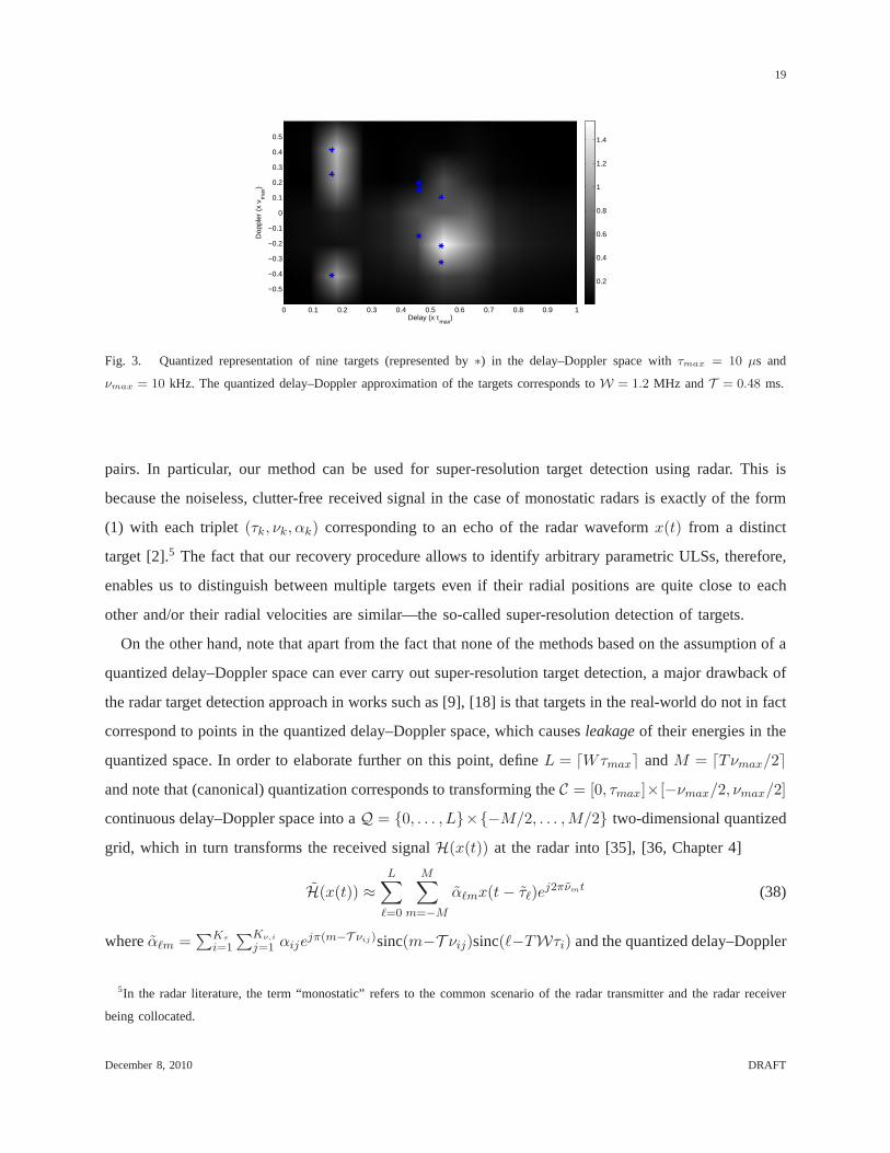
Fig. 3. Quantized representation of nine targets (represented by ∗) in the delay–Doppler space withτmax = 10 µs and

νmax = 10 kHz. The quantized delay–Doppler approximation of the targets corresponds toW = 1.2 MHz andT = 0.48 ms.

pairs. In particular, our method can be used for super-resolution target detection using radar. This is

because the noiseless, clutter-free received signal in thecase of monostatic radars is exactly of the form

(1) with each triplet(τk, νk, αk) corresponding to an echo of the radar waveformx(t) from a distinct

target [2].5 The fact that our recovery procedure allows to identify arbitrary parametric ULSs, therefore,

enables us to distinguish between multiple targets even if their radial positions are quite close to each

other and/or their radial velocities are similar—the so-called super-resolution detection of targets.

On the other hand, note that apart from the fact that none of the methods based on the assumption of a

quantized delay–Doppler space can ever carry out super-resolution target detection, a major drawback of

the radar target detection approach in works such as [9], [18] is that targets in the real-world do not in fact

correspond to points in the quantized delay–Doppler space,which causesleakageof their energies in the

quantized space. In order to elaborate further on this point, defineL = ⌈Wτmax⌉ andM = ⌈Tνmax/2⌉and note that (canonical) quantization corresponds to transforming theC = [0, τmax]×[−νmax/2, νmax/2]

continuous delay–Doppler space into aQ = 0, . . . , L×−M/2, . . . ,M/2 two-dimensional quantized

grid, which in turn transforms the received signalH(x(t)) at the radar into [35], [36, Chapter 4]

H(x(t)) ≈L∑

ℓ=0

M∑

m=−M

αℓmx(t− τℓ)ej2πνmt (38)

whereαℓm =∑Kτ

i=1

∑Kν,i

j=1 αijejπ(m−T νij)sinc(m−T νij)sinc(ℓ−TWτi) and the quantized delay–Doppler

5In the radar literature, the term “monostatic” refers to thecommon scenario of the radar transmitter and the radar receiver

being collocated.


20

0 0.1 0.2 0.3 0.4 0.5 0.6 0.7 0.8 0.9 1−0.5

−0.4

−0.3

−0.2

−0.1

0

0.1

0.2

0.3

0.4

0.5

Delay (x τmax

)

Dop

pler

(x

ν max

)

0.1

0.2

0.3

0.4

0.5

0.6

0.7

0.8

0.9

1True TargetsMF Peaks

(a)

0 0.1 0.2 0.3 0.4 0.5 0.6 0.7 0.8 0.9 1−0.5

−0.4

−0.3

−0.2

−0.1

0

0.1

0.2

0.3

0.4

0.5

Delay (x τmax

)

Dop

pler

(x

ν max

)

True TargetsEstimated Targets

(b)

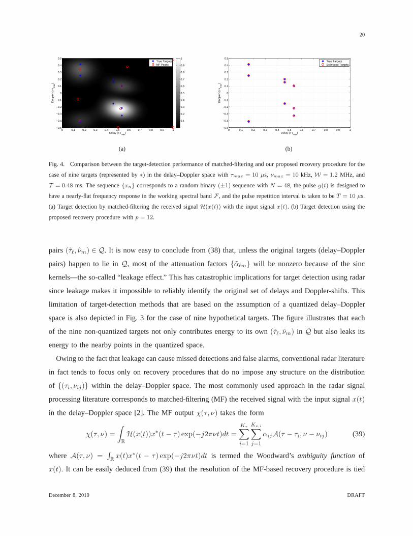
Fig. 4. Comparison between the target-detection performance of matched-filtering and our proposed recovery procedurefor the

case of nine targets (represented by∗) in the delay–Doppler space withτmax = 10 µs, νmax = 10 kHz, W = 1.2 MHz, and

T = 0.48 ms. The sequencexn corresponds to a random binary(±1) sequence withN = 48, the pulseg(t) is designed to

have a nearly-flat frequency response in the working spectral bandF , and the pulse repetition interval is taken to beT = 10 µs.

(a) Target detection by matched-filtering the received signal H(x(t)) with the input signalx(t). (b) Target detection using the

proposed recovery procedure withp = 12.

pairs(τℓ, νm) ∈ Q. It is now easy to conclude from (38) that, unless the original targets (delay–Doppler

pairs) happen to lie inQ, most of the attenuation factorsαℓm will be nonzero because of the sinc

kernels—the so-called “leakage effect.” This has catastrophic implications for target detection using radar

since leakage makes it impossible to reliably identify the original set of delays and Doppler-shifts. This

limitation of target-detection methods that are based on the assumption of a quantized delay–Doppler

space is also depicted in Fig. 3 for the case of nine hypothetical targets. The figure illustrates that each

of the nine non-quantized targets not only contributes energy to its own(τℓ, νm) in Q but also leaks its

energy to the nearby points in the quantized space.

Owing to the fact that leakage can cause missed detections and false alarms, conventional radar literature

in fact tends to focus only on recovery procedures that do no impose any structure on the distribution

of (τi, νij) within the delay–Doppler space. The most commonly used approach in the radar signal

processing literature corresponds to matched-filtering (MF) the received signal with the input signalx(t)

in the delay–Doppler space [2]. The MF outputχ(τ, ν) takes the form

χ(τ, ν) =

∫

R

H(x(t))x∗(t− τ) exp(−j2πνt)dt =Kτ∑

i=1

Kν,i∑

j=1

αijA(τ − τi, ν − νij) (39)

where A(τ, ν) =∫Rx(t)x∗(t − τ) exp(−j2πνt)dt is termed the Woodward’sambiguity functionof

x(t). It can be easily deduced from (39) that the resolution of theMF-based recovery procedure is tied


21

0 0.1 0.2 0.3 0.4 0.5 0.6 0.7 0.8 0.9 1−0.5

−0.4

−0.3

−0.2

−0.1

0

0.1

0.2

0.3

0.4

0.5

Delay (x τmax

)

Dop

pler

(x

ν max

)

Fig. 5. Delay–Doppler representation of a parametric ULSH corresponding toK = 6 delay–Doppler pairs withτmax = 10 µs

andνmax = 10 kHz.

to the supportof the ambiguity function in the delay–Doppler space. Ideally, one would like to have

A(τ, ν) = δ(τ)δ(ν) for super-resolution detection of targets but two fundamental properties of ambiguity

functions, namely,|A(0, 0)|2 =∫|x(t)|2dt and

∫∫|A(τ, ν)|2dτdν =

∫|x(t)|2dt, dictate that no real-

world signalx(t) can yield infinitesimally-fine resolution in this case either [2]. In fact, the resolution

of MF-based recovery techniques also tends to be on the orderof W−1 andT −1 in the delay space and

the Doppler space, respectively, which severely limits their ability to distinguish between two closely-

spaced targets in the delay–Doppler space. This inability of MF-based methods to resolve closely-spaced

delay–Doppler pairs is depicted in Fig. 4. This figure compares the target-detection performance of MF

and the recovery procedure proposed in this paper for the case of nine closely-spaced targets. It is easy

to see from Fig. 4(a) that matched-filtering the received signal H(x(t)) with the input signalx(t) gives

rise to peaks that are not centered at the true targets for a majority of the targets. On the other hand,

Fig. 4(b) illustrates that our recovery procedure correctly identifies the locations of all nine of the targets

in the delay–Doppler space.

VII. N UMERICAL EXPERIMENTS

In this section, we explore various issues using numerical experiments that were not treated theoretically

earlier in the paper. These include robustness of our methodin the presence of noise and the effects

of truncated digital filters, use of finite number of samples,choice of probing sequencexn, and

model-order mismatch on the recovery performance. Throughout this section, the numerical experiments

correspond to a parametric ULSH that is described by a total ofK = 6 delay–Doppler pairs with


22

Kτ = 2 andKν,1 = Kν,2 = 3. The locations of these pairs in the delay–Doppler space aregiven by

Fig. 5, while the attenuation factors associated with each of the six delay–Doppler pairs are taken to have

unit amplitudes and random phases.

In order to identifyH, we design the prototype pulseg(t) to have a constant frequency response over

the working spectral bandF =[− π

T p,πT p

]with p = 4 andT = 10 µs, that is,G(ω) ≈ 1 whenω ∈ F

andG(ω) ≈ 0 whenω /∈ F . In other words, the input signalx(t) is chosen to have bandwidthW = 8πT .

In addition, unless otherwise noted, we use a probing sequencexn corresponding to a random binary

(±1) sequence withN = 30, which leads to a time–bandwidth product ofT W ≈ 240π. Note that the

chosen time–bandwidth product here is more than the lower bound of Theorem 2 by a factor of5 so as

to increase the robustness to noise. Also, unless otherwisestated, all experiments in the following use an

ideal (flat) LPF as the sampling filter (cf. Fig. 2). We use the ESPRIT method described in Section III

for recovery of the delays and the matrix-pencil method [13]for recovery of the corresponding Doppler-

shifts. Given the rich history of these two subspace methods, there exist many standard techniques in

the literature (see, e.g., [37], [38]) for providing them with reliable estimates of the model orders in

the presence of noise. As such, we assume in the following that both these methods have access to

correct values ofKτ andKν,i’s. Finally, the performance metrics that we use in this section are the

(normalized) mean-squared error (MSE) of the estimated delays and Doppler-shifts (averaged over100

noise realizations), defined as

e2delay =1

2

2∑

i=1

[(τi − τi)/τmax

]2, (40)

and

e2Doppler =1

6

2∑

i=1

3∑

j=1

[(νij − νij)/νmax

]2, (41)

whereτi and νij denote the estimated delays and Doppler-shifts, respectively.

1) Robustness to Noise:We first examine the robustness of our method when the received signal

H(x(t)) is corrupted by additive noise. The results of this experiment are shown in Fig. 6, which plots

the MSE of the estimated delays and Doppler-shifts as a function of the SNR. It can be seen from the

figure that the ability of the proposed procedure to resolve delay–Doppler pairs is primarily a function

of the SNR and its performance degrades gracefully in the presence of noise.

2) Effects of Truncated Digital-Correction Filter Banks:Recall from Section III that our recovery

method is composed of various digital-correction stages (see also Fig. 2). The filters used in these stages,

which includeφℓ[n] and ψℓ[n], have infinite impulse responses in general so that their practical


23

0 10 20 30 40 50 60−90

−80

−70

−60

−50

−40

−30

−20

−10

0

10

Signal−to−Noise Ratio (dB)

Mea

n S

quar

ed E

rror

(dB

)

Doppler−ShiftsDelays

Fig. 6. Mean-squared error of the estimated delays and Doppler-shifts as a function of the signal-to-noise ratio.

0 10 20 30 40 50 60−90

−80

−70

−60

−50

−40

−30

−20

−10

0


Mea

n S

quar

ed E

rror

(dB

)

Estimation of Delays

1 Tap11 Taps35 Taps49 Taps

(a)

0 10 20 30 40 50 60−60

−50

−40

−30

−20

−10

0

10


Mea

n S

quar

ed E

rror

(dB

)

Estimation of Doppler−Shifts

1 Tap11 Taps35 Taps49 Taps

(b)

Fig. 7. Mean-squared error of the estimated delays and Doppler-shifts as a function of the signal-to-noise ratio for various

lengths of the impulse responses of the filters.

implementation requires truncation of their impulse responses. The truncated lengths of these filters also

determine the (computational) delay and the computationalload of the proposed procedure. Fig. 7 plots

the MSE of the estimated delays (Fig. 7(a)) and Doppler-shifts (Fig. 7(b)) as a function of the SNR for

various lengths of the impulse responses of the filters. There are two important insights that can be drawn

from the results of this experiment. First, for a fixed lengthof the impulse responses, there is always some

SNR beyond which the estimation error caused by the truncation of the impulse responses becomes more

dominant than the error caused by the additive noise (as evident by the error floors in Fig. 7). Second,

and perhaps most importantly, filters with49 taps seem to provide good estimation accuracy up to an

SNR of 60 dB, whereas filters with even just35 taps yield good estimates at SNRs below50 dB.


24

0 10 20 30 40 50 60 70 80−100

−90

−80

−70

−60

−50

−40

−30

−20

−10


Mea

n S

quar

ed E

rror

(dB

)Estimation of Delays

120 Samples Used152 Samples Used184 Samples Used248 Samples Used

(a)

0 10 20 30 40 50 60 70 80−80

−70

−60

−50

−40

−30

−20

−10

0

10


Mea

n S

quar

ed E

rror

(dB

)



(b)

Fig. 8. Mean-squared error of the estimated delays and Doppler-shifts as a function of the signal-to-noise ratio for different

numbers of samples collected at the output of the sampling filter (corresponding to an ideal low-pass filter).

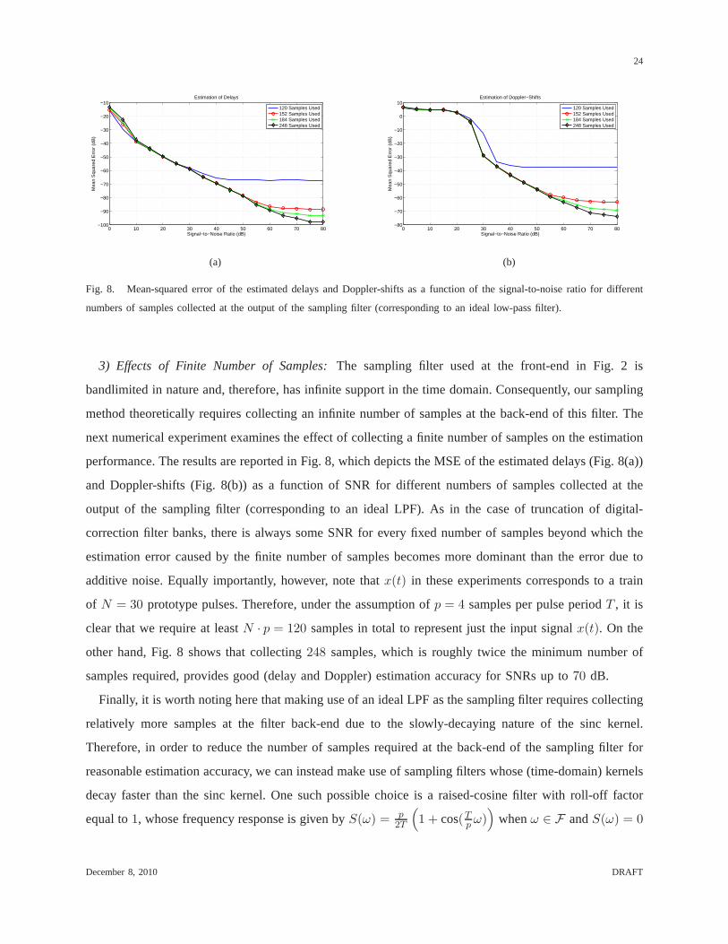
3) Effects of Finite Number of Samples:The sampling filter used at the front-end in Fig. 2 is

bandlimited in nature and, therefore, has infinite support in the time domain. Consequently, our sampling

method theoretically requires collecting an infinite number of samples at the back-end of this filter. The

next numerical experiment examines the effect of collecting a finite number of samples on the estimation

performance. The results are reported in Fig. 8, which depicts the MSE of the estimated delays (Fig. 8(a))

and Doppler-shifts (Fig. 8(b)) as a function of SNR for different numbers of samples collected at the

output of the sampling filter (corresponding to an ideal LPF). As in the case of truncation of digital-

correction filter banks, there is always some SNR for every fixed number of samples beyond which the

estimation error caused by the finite number of samples becomes more dominant than the error due to

additive noise. Equally importantly, however, note thatx(t) in these experiments corresponds to a train

of N = 30 prototype pulses. Therefore, under the assumption ofp = 4 samples per pulse periodT , it is

clear that we require at leastN · p = 120 samples in total to represent just the input signalx(t). On the

other hand, Fig. 8 shows that collecting248 samples, which is roughly twice the minimum number of

samples required, provides good (delay and Doppler) estimation accuracy for SNRs up to70 dB.

Finally, it is worth noting here that making use of an ideal LPF as the sampling filter requires collecting

relatively more samples at the filter back-end due to the slowly-decaying nature of the sinc kernel.

Therefore, in order to reduce the number of samples requiredat the back-end of the sampling filter for

reasonable estimation accuracy, we can instead make use of sampling filters whose (time-domain) kernels

decay faster than the sinc kernel. One such possible choice is a raised-cosine filter with roll-off factor

equal to1, whose frequency response is given byS(ω) = p2T

(1 + cos(Tp ω)

)whenω ∈ F andS(ω) = 0


25

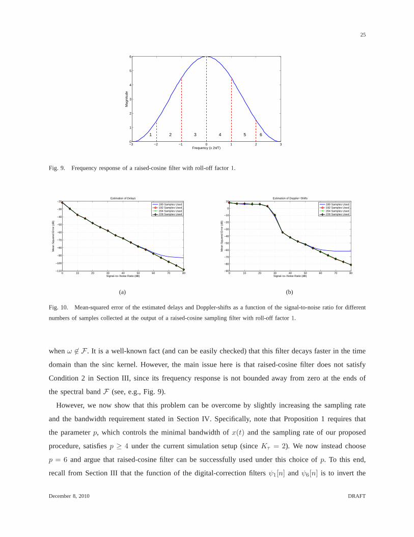
−3 −2 −1 0 1 2 30

1

2

3

4

5

6

1 2 3 4 5 6

Frequency (x 2π/T)

Mag

nitu

de

Fig. 9. Frequency response of a raised-cosine filter with roll-off factor 1.

0 10 20 30 40 50 60 70 80−110

−100

−90

−80

−70

−60

−50

−40

−30

−20


Mea

n S

quar

ed E

rror

(dB

)

Estimation of Delays


(a)

0 10 20 30 40 50 60 70 80−90

−80

−70

−60

−50

−40

−30

−20

−10

0

10


Mea

n S

quar

ed E

rror

(dB

)



(b)

Fig. 10. Mean-squared error of the estimated delays and Doppler-shifts as a function of the signal-to-noise ratio for different

numbers of samples collected at the output of a raised-cosine sampling filter with roll-off factor1.

whenω 6∈ F . It is a well-known fact (and can be easily checked) that thisfilter decays faster in the time

domain than the sinc kernel. However, the main issue here is that raised-cosine filter does not satisfy

Condition 2 in Section III, since its frequency response is not bounded away from zero at the ends of

the spectral bandF (see, e.g., Fig. 9).

However, we now show that this problem can be overcome by slightly increasing the sampling rate

and the bandwidth requirement stated in Section IV. Specifically, note that Proposition 1 requires that

the parameterp, which controls the minimal bandwidth ofx(t) and the sampling rate of our proposed

procedure, satisfiesp ≥ 4 under the current simulation setup (sinceKτ = 2). We now instead choose

p = 6 and argue that raised-cosine filter can be successfully usedunder this choice ofp. To this end,

recall from Section III that the function of the digital-correction filtersψ1[n] andψ6[n] is to invert the


26

0 10 20 30 40 50 60 70 80 90 100−80

−70

−60

−50

−40

−30

−20

−10


Mea

n S

quar

ed E

rror

(dB

)Estimation of Delays

Repetition: 1Repetition: 2Repetition: 4Repetition: 32

(a)

0 10 20 30 40 50 60 70 80 90 100−60

−50

−40

−30

−20

−10

0

10


Mea

n S

quar

ed E

rror

(dB

)


Repetition: 1Repetition: 2Repetition: 4Repetition: 32

(b)

Fig. 11. Mean-squared error of the estimated delays and Doppler-shifts as a function of the signal-to-noise ratio for various

probing sequences.

frequency response of the sampling kernel corresponding tothe frequency bands denoted by1 and6 in

Fig. 9, respectively (under the assumption that the pulseg(t) has a flat frequency response). In the case

of a raised-cosine filter, however, we cannot compensate forthe non-flat nature of these two bands since

they are not bounded away from zero. Nevertheless, because of the fact that we are usingp = 6, we can

simply disregard channels1 and 6 after the first digital-correction stage and work with the rest of the

four channels (2-4) only. We make use of this insight to repeat the last numerical experiment using a

raised-cosine filter and report the results in Fig. 10. It is easy to see from Fig. 10 that, despite increasing

p to 6, raised-cosine filter performs better than an ideal LPF using fewer samples.

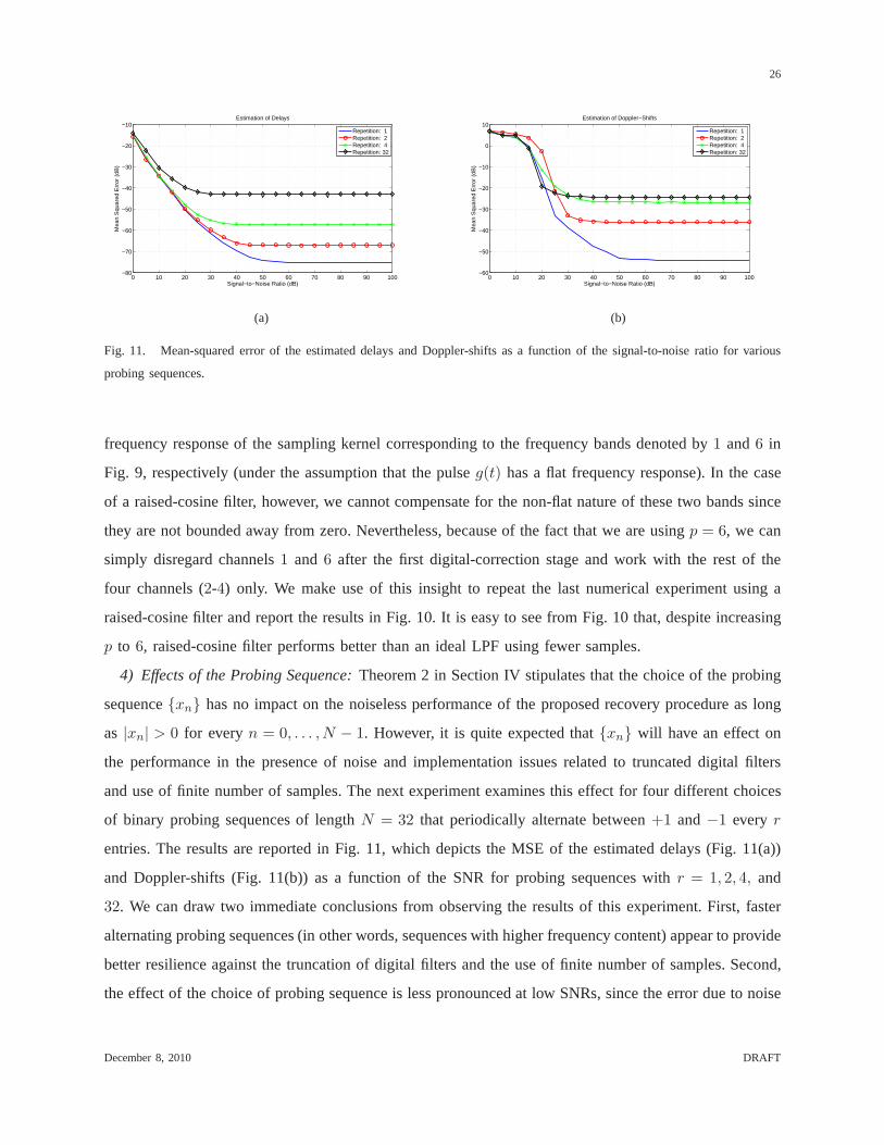
4) Effects of the Probing Sequence:Theorem 2 in Section IV stipulates that the choice of the probing

sequencexn has no impact on the noiseless performance of the proposed recovery procedure as long

as |xn| > 0 for everyn = 0, . . . , N − 1. However, it is quite expected thatxn will have an effect on

the performance in the presence of noise and implementationissues related to truncated digital filters

and use of finite number of samples. The next experiment examines this effect for four different choices

of binary probing sequences of lengthN = 32 that periodically alternate between+1 and−1 every r

entries. The results are reported in Fig. 11, which depicts the MSE of the estimated delays (Fig. 11(a))

and Doppler-shifts (Fig. 11(b)) as a function of the SNR for probing sequences withr = 1, 2, 4, and

32. We can draw two immediate conclusions from observing the results of this experiment. First, faster

alternating probing sequences (in other words, sequences with higher frequency content) appear to provide

better resilience against the truncation of digital filtersand the use of finite number of samples. Second,

the effect of the choice of probing sequence is less pronounced at low SNRs, since the error due to noise


27

0 0.1 0.2 0.3 0.4 0.5 0.6 0.7 0.8 0.9 1−0.5

−0.4

−0.3

−0.2

−0.1

0

0.1

0.2

0.3

0.4

0.5

Delay (x τmax

)

Dop

pler

(x

ν max

)

True Delay−Doppler PairsEstimated Delay−Doppler Pairs

Fig. 12. Effects of model-order mismatch on the performanceof the proposed recovery procedure corresponding toH with

K = 14 delay–Doppler pairs.

at low SNRs dominates the errors caused by other implementation imperfections.

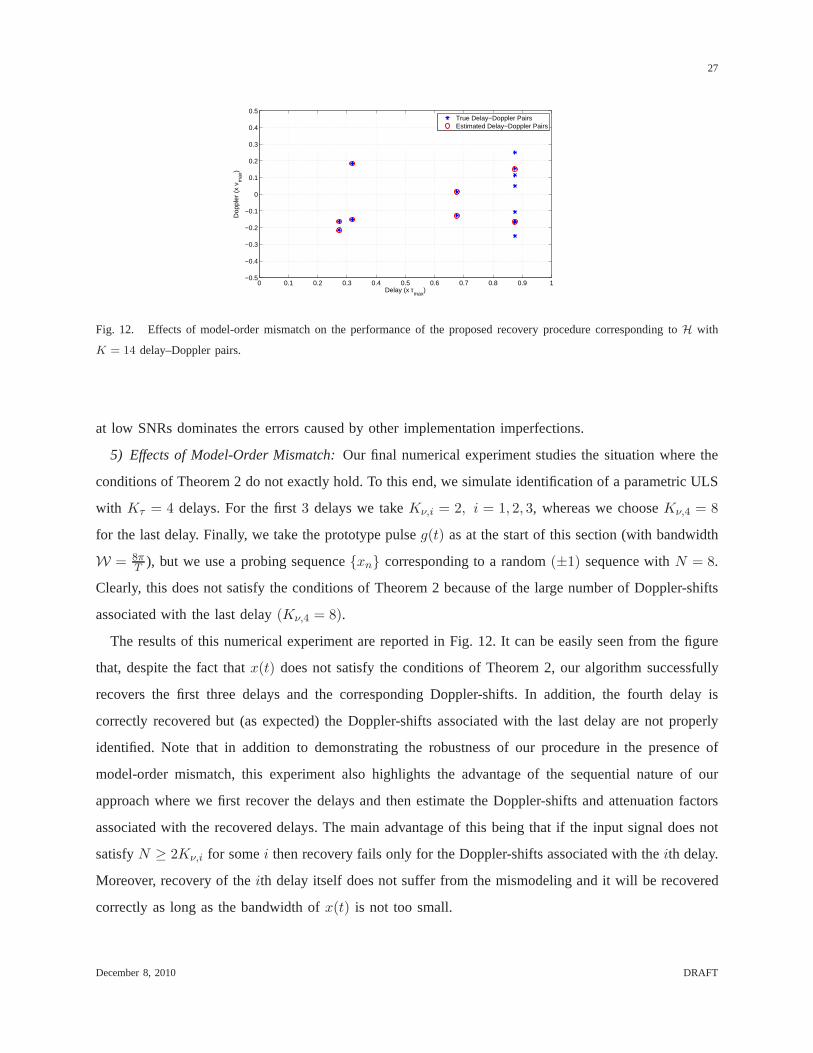
5) Effects of Model-Order Mismatch:Our final numerical experiment studies the situation where the

conditions of Theorem 2 do not exactly hold. To this end, we simulate identification of a parametric ULS

with Kτ = 4 delays. For the first3 delays we takeKν,i = 2, i = 1, 2, 3, whereas we chooseKν,4 = 8

for the last delay. Finally, we take the prototype pulseg(t) as at the start of this section (with bandwidth

W = 8πT ), but we use a probing sequencexn corresponding to a random(±1) sequence withN = 8.

Clearly, this does not satisfy the conditions of Theorem 2 because of the large number of Doppler-shifts

associated with the last delay(Kν,4 = 8).

The results of this numerical experiment are reported in Fig. 12. It can be easily seen from the figure

that, despite the fact thatx(t) does not satisfy the conditions of Theorem 2, our algorithm successfully

recovers the first three delays and the corresponding Doppler-shifts. In addition, the fourth delay is

correctly recovered but (as expected) the Doppler-shifts associated with the last delay are not properly

identified. Note that in addition to demonstrating the robustness of our procedure in the presence of

model-order mismatch, this experiment also highlights theadvantage of the sequential nature of our

approach where we first recover the delays and then estimate the Doppler-shifts and attenuation factors

associated with the recovered delays. The main advantage ofthis being that if the input signal does not

satisfyN ≥ 2Kν,i for somei then recovery fails only for the Doppler-shifts associatedwith the ith delay.

Moreover, recovery of theith delay itself does not suffer from the mismodeling and it will be recovered

correctly as long as the bandwidth ofx(t) is not too small.


28

VIII. C ONCLUSION

In this paper, we revisited the problem of identification of parametric underspread linear systems that

are completely described by a finite set of delays and Doppler-shifts. We established that sufficiently-

underspread parametric linear systems are identifiable as long as the time–bandwidth product of the

input signal is proportional to the square of the total number of delay–Doppler pairs. In addition, we

concretely specified the nature of the input signal and the structure of a corresponding polynomial-

time recovery procedure that enable identification of parametric underspread linear systems. Extensive

simulation results confirm that—as long as the time–bandwidth product of the input signal satisfies the

requisite conditions—the proposed recovery procedure is quite robust to noise and other implementation

issues. This makes our algorithm extremely useful for application areas in which the system performance

depends critically on the ability to resolve closely spaceddelay–Doppler pairs. In particular, our proposed

identification method can be used for super-resolution target detection using radar.

REFERENCES

[1] J. G. Proakis,Digital Communications, 4th ed. New York, NY: McGraw-Hill, 2001.

[2] M. I. Skolnik, Introduction to Radar Systems, 3rd ed. New York, NY: McGraw-Hill, 2001.

[3] W. Kozek and G. E. Pfander, “Identification of operators with bandlimited symbols,”SIAM J. Math. Anal., vol. 37, no. 3,

pp. 867–888, 2005.

[4] T. Kailath, “Measurements on time-variant communication channels,”IRE Trans. Inform. Theory, vol. 8, no. 5, pp. 229–236,

Sep. 1962.

[5] P. Bello, “Measurement of random time-variant linear channels,”IEEE Trans. Inform. Theory, vol. 15, no. 4, pp. 469–475,

Jul. 1969.

[6] G. E. Pfander and D. F. Walnut, “Measurement of time-variant linear channels,”IEEE Trans. Inform. Theory, vol. 52,

no. 11, pp. 4808–4820, Nov. 2006.

[7] W. U. Bajwa, J. Haupt, A. M. Sayeed, and R. Nowak, “Compressed channel sensing: A new approach to estimating sparse

multipath channels,”Proc. IEEE, vol. 98, no. 6, pp. 1058–1076, Jun. 2010.

[8] D. Slepian, “On bandwidth,”Proc. IEEE, vol. 64, no. 3, pp. 292–300, Mar. 1976.

[9] M. A. Herman and T. Strohmer, “High-resolution radar viacompressed sensing,”IEEE Trans. Signal Processing, vol. 57,

no. 6, pp. 2275–2284, Jun. 2009.

[10] K. Gedalyahu and Y. C. Eldar, “Time-delay estimation from low-rate samples: A union of subspaces approach,”IEEE

Trans. Signal Processing, vol. 58, no. 6, pp. 3017–3031, Jun. 2010.

[11] D. W. Tufts and R. Kumaresan, “Estimation of frequencies of multiple sinusoids: Making linear prediction perform like

maximum likelihood,”Proc. IEEE, vol. 70, no. 9, pp. 975–989, Sep. 1982.

[12] R. Roy, A. Paulraj, and T. Kailath, “ESPRIT—A subspace rotation approach to estimation of parameters of cisoids in

noise,” IEEE Trans. Acoust., Speech, Signal Processing, vol. 34, no. 5, pp. 1340–1342, Oct. 1986.

[13] Y. Hua and T. K. Sarkar, “Matrix pencil method for estimating parameters of exponentially damped/undamped sinusoids

in noise,” IEEE Trans. Acoust., Speech, Signal Processing, vol. 38, no. 5, pp. 814–824, May 1990.


29

[14] P. Stoica and R. L. Moses,Introduction to Spectral Analysis. Englewood Cliffs, NJ: Prentice-Hall, 1997.

[15] A. W. Habboosh, R. J. Vaccaro, and S. Kay, “An algorithm for detecting closely spaced delay/Doppler components,” in

Proc. IEEE Int. Conf. Acoustics, Speech and Signal Processing (ICASSP’97), Munich, Germany, Apr. 1997, pp. 535–538.

[16] I. C. Wong and B. L. Evans, “Low-complexity adaptive high-resolution channel prediction for OFDM systems,” inProc.

IEEE Global Telecommunications Conf. (GLOBECOM’06), San Francisco, CA, Dec. 2006, pp. 1–5.

[17] W. U. Bajwa, A. M. Sayeed, and R. Nowak, “Learning sparsedoubly-selective channels,” inProc. 45th Annu. Allerton

Conf. Communication, Control, and Computing, Monticello, IL, Sep. 2008, pp. 575–582.

[18] X. Tan, W. Roberts, J. Li, and P. Stoica, “Range-Dopplerimaging via a train of probing pulses,”IEEE Trans. Signal

Processing, vol. 57, no. 3, pp. 1084–1097, Mar. 2009.

[19] A. Jakobsson, A. L. Swindlehurst, and P. Stoica, “Subspace-based estimation of time delays and Doppler shifts,”IEEE

Trans. Signal Processing, vol. 46, no. 9, pp. 2472–2483, Sep. 1998.

[20] M. Mishali, Y. C. Eldar, O. Dounaevsky, and E. Shoshan, “Xampling: Analog to digital at sub-Nyquist rates,” CCIT

Report # 751, EE Dept., Technion—Israel Institute of Technology, Dec. 2009. [Online]. Available: arXiv:0912.2495

[21] M. Mishali, Y. C. Eldar, and A. Elron, “Xampling: Signalacquisition and processing in union of subspaces,” CCIT

Report # 747, EE Dept., Technion—Israel Institute of Technology, Oct. 2009. [Online]. Available: arXiv:0911.0519

[22] M. Mishali and Y. C. Eldar, “From theory to practice: Sub-Nyquist sampling of sparse wideband analog signals,”IEEE J.

Select. Topics Signal Processing, vol. 4, no. 2, pp. 375–391, Apr. 2010.

[23] ——, “Blind multi-band signal reconstruction: Compressed sensing for analog signals,”IEEE Trans. Signal Processing,

vol. 57, no. 3, pp. 993–1009, Mar. 2009.

[24] Y. C. Eldar, “Compressed sensing of analog signals in shift-invariant spaces,”IEEE Trans. Signal Processing, vol. 57,

no. 8, pp. 2986–2997, Aug. 2009.

[25] Y. C. Eldar and M. Mishali, “Robust recovery of signals from a structured union of subspaces,”IEEE Trans. Inform.

Theory, vol. 55, no. 11, pp. 5302–5316, Nov. 2009.

[26] E. Moulines, P. Duhamel, J. Cardoso, S. Mayrargue, and T. Paris, “Subspace methods for the blind identification of

multichannel FIR filters,”IEEE Trans. Signal Processing, vol. 43, no. 2, pp. 516–25, Feb. 1995.

[27] H. Krim and M. Viberg, “Two decades of array signal processing research: The parametric approach,”IEEE Signal

Processing Mag., vol. 13, no. 4, pp. 67–94, Jul. 1996.

[28] R. Roy and T. Kailath, “ESPRIT—Estimation of signal parameters via rotational invariance techniques,”IEEE Trans.

Acoust., Speech, Signal Processing, vol. 37, no. 7, pp. 984–995, Jul. 1989.

[29] T.-J. Shan, M. Wax, and T. Kailath, “On spatial smoothing for direction-of-arrival estimation of coherent signals,” IEEE

Trans. Acoust., Speech, Signal Processing, vol. 33, no. 4, pp. 806–811, Aug. 1985.

[30] P. L. Dragotti, M. Vetterli, and T. Blu, “Sampling moments and reconstructing signals of finite rate of innovation: Shannon

meets Strang-Fix,”IEEE Trans. Signal Processing, vol. 55, no. 5, pp. 1741–1757, May 2007.

[31] M. Vetterli, P. Marziliano, and T. Blu, “Sampling signals with finite rate of innovation,”IEEE Trans. Signal Processing,

vol. 50, no. 6, pp. 1417–1428, Jun. 2002.

[32] R. Tur, K. Gedalyahu, and Y. C. Eldar, “Multichannel sampling of pulse streams at the rate of innovation,” submittedto

IEEE Trans. Signal Processing. [Online]. Available: arXiv:1004.5070

[33] R. Tur, Y. C. Eldar, and Z. Friedman, “Low rate sampling of pulse streams with application to ultrasound imaging,”

submitted toIEEE Trans. Signal Processing. [Online]. Available: arXiv:1003.2822

[34] G. E. Pfander and H. Rauhut, “Sparsity in time-frequency representations,”J. Fourier Anal. Appl., Aug. 2009.


arXiv:0912.2495

arXiv:0911.0519

arXiv:1004.5070

arXiv:1003.2822

30

[35] P. Bello, “Characterization of randomly time-variantlinear channels,”IEEE Trans. Commun., vol. 11, no. 4, pp. 360–393,

Dec. 1963.

[36] W. U. Bajwa, “New information processing theory and methods for exploiting sparsity in wireless systems,” Ph.D.

dissertation, University of Wisconsin-Madison, Madison,WI, 2009.

[37] M. Wax, “Detection and estimation of superimposed signals,” Ph.D. dissertation, Stanford University, Stanford,CA, 1985.

[38] R. H. Roy, “ESPRIT—estimation of signal parameters viarotational invariance techniques,” Ph.D. dissertation, Stanford

University, Stanford, CA, 1987.


1 identiﬁcation of parametric underspread linear...

Documents