1

Inferring rudimentary rules

1R: learns a 1-level decision tree I.e., rules that all test one particular attribute

Basic version One branch for each value Each branch assigns most frequent class Error rate: proportion of instances that don’t

belong to the majority class of their corresponding branch

Choose attribute with lowest error rate

(assumes nominal attributes)

2

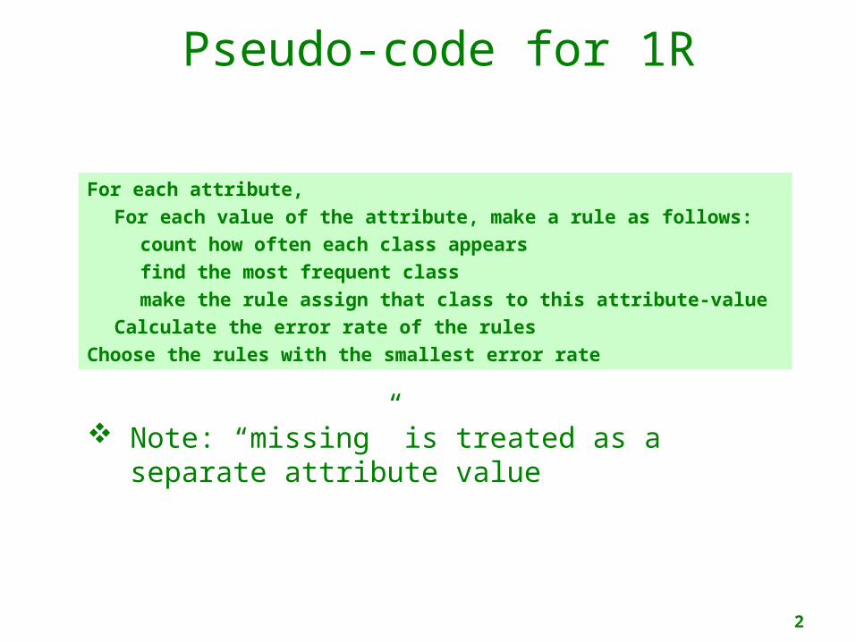
Pseudo-code for 1R

For each attribute,

For each value of the attribute, make a rule as follows:

count how often each class appears

find the most frequent class

make the rule assign that class to this attribute-value

Calculate the error rate of the rules

Choose the rules with the smallest error rate

Note: “missing” is treated as a separate attribute value

3

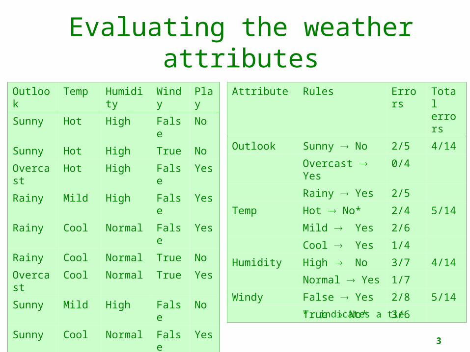
Evaluating the weather attributes

Attribute Rules Errors

Total errors

Outlook Sunny No 2/5 4/14

Overcast Yes

0/4

Rainy Yes 2/5

Temp Hot No* 2/4 5/14

Mild Yes 2/6

Cool Yes 1/4

Humidity High No 3/7 4/14

Normal Yes 1/7

Windy False Yes 2/8 5/14

True No* 3/6

Outlook Temp Humidity

Windy

Play

Sunny Hot High False No

Sunny Hot High True No

Overcast

Hot High False Yes

Rainy Mild High False Yes

Rainy Cool Normal False Yes

Rainy Cool Normal True No

Overcast

Cool Normal True Yes

Sunny Mild High False No

Sunny Cool Normal False Yes

Rainy Mild Normal False Yes

Sunny Mild Normal True Yes

Overcast

Mild High True Yes

Overcast

Hot Normal False Yes

Rainy Mild High True No

* indicates a tie

4

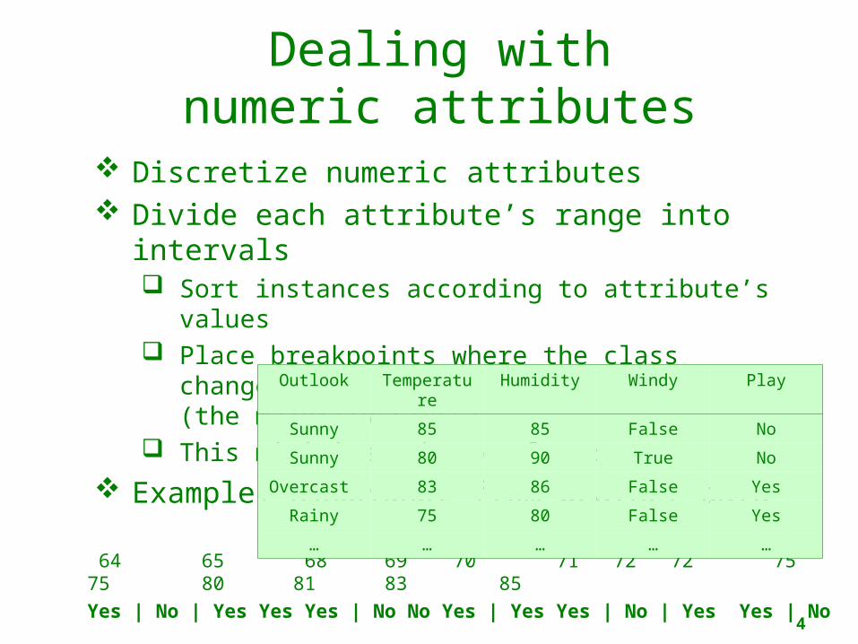
Dealing withnumeric attributes

Discretize numeric attributes Divide each attribute’s range into

intervals Sort instances according to attribute’s values Place breakpoints where the class changes

(the majority class) This minimizes the total error

Example: temperature from weather data

64 65 68 69 70 71 72 72 75 75 80 81 83 85Yes | No | Yes Yes Yes | No No Yes | Yes Yes | No | Yes Yes | No

Outlook Temperature

Humidity Windy Play

Sunny 85 85 False No

Sunny 80 90 True No

Overcast 83 86 False Yes

Rainy 75 80 False Yes

… … … … …

5

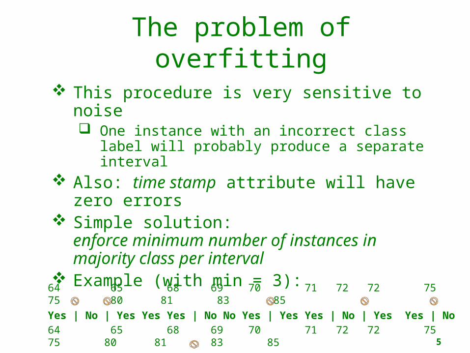
The problem of overfitting

This procedure is very sensitive to noise One instance with an incorrect class label

will probably produce a separate interval Also: time stamp attribute will have zero

errors Simple solution:

enforce minimum number of instances in majority class per interval

Example (with min = 3):

64 65 68 69 70 71 72 72 75 75 80 81 83 85Yes | No | Yes Yes Yes | No No Yes | Yes Yes | No | Yes Yes | No64 65 68 69 70 71 72 72 75 75 80 81 83 85Yes No Yes Yes Yes | No No Yes Yes Yes | No Yes Yes No

6

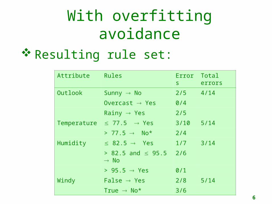
With overfitting avoidance

Resulting rule set:

Attribute Rules Errors Total errors

Outlook Sunny No 2/5 4/14

Overcast Yes 0/4

Rainy Yes 2/5

Temperature 77.5 Yes 3/10 5/14

> 77.5 No* 2/4

Humidity 82.5 Yes 1/7 3/14

> 82.5 and 95.5 No

2/6

> 95.5 Yes 0/1

Windy False Yes 2/8 5/14

True No* 3/6

7

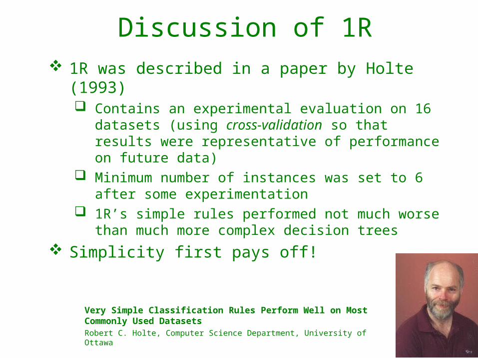
Discussion of 1R 1R was described in a paper by Holte

(1993) Contains an experimental evaluation on 16

datasets (using cross-validation so that results were representative of performance on future data)

Minimum number of instances was set to 6 after some experimentation

1R’s simple rules performed not much worse than much more complex decision trees

Simplicity first pays off!

Very Simple Classification Rules Perform Well on Most Commonly Used DatasetsRobert C. Holte, Computer Science Department, University of Ottawa

8

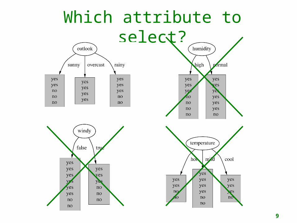
Constructing decision trees

Strategy: top downRecursive divide-and-conquer fashion First: select attribute for root node

Create branch for each possible attribute value

Then: split instances into subsetsOne for each branch extending from the node

Finally: repeat recursively for each branch, using only instances that reach the branch

Stop if all instances have the same class

9

Which attribute to select?

10

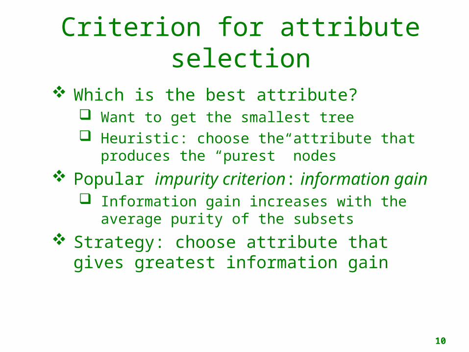
Criterion for attribute selection

Which is the best attribute? Want to get the smallest tree Heuristic: choose the attribute that

produces the “purest” nodes

Popular impurity criterion: information gain Information gain increases with the

average purity of the subsets

Strategy: choose attribute that gives greatest information gain

11

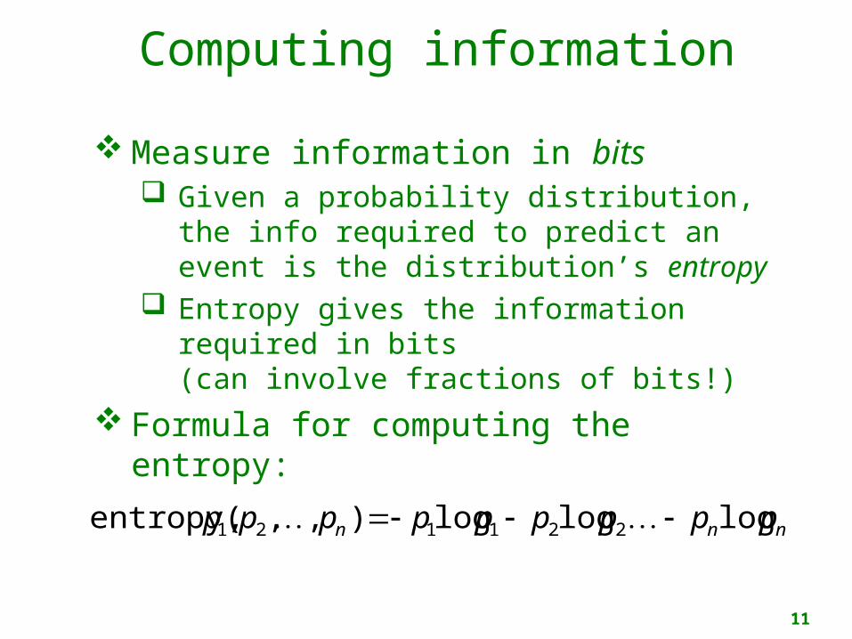
Computing information

Measure information in bits Given a probability distribution, the

info required to predict an event is the distribution’s entropy

Entropy gives the information required in bits(can involve fractions of bits!)

Formula for computing the entropy:

entropy(p1, p2,, pn ) p1logp1 p2logp2 pnlogpn

12

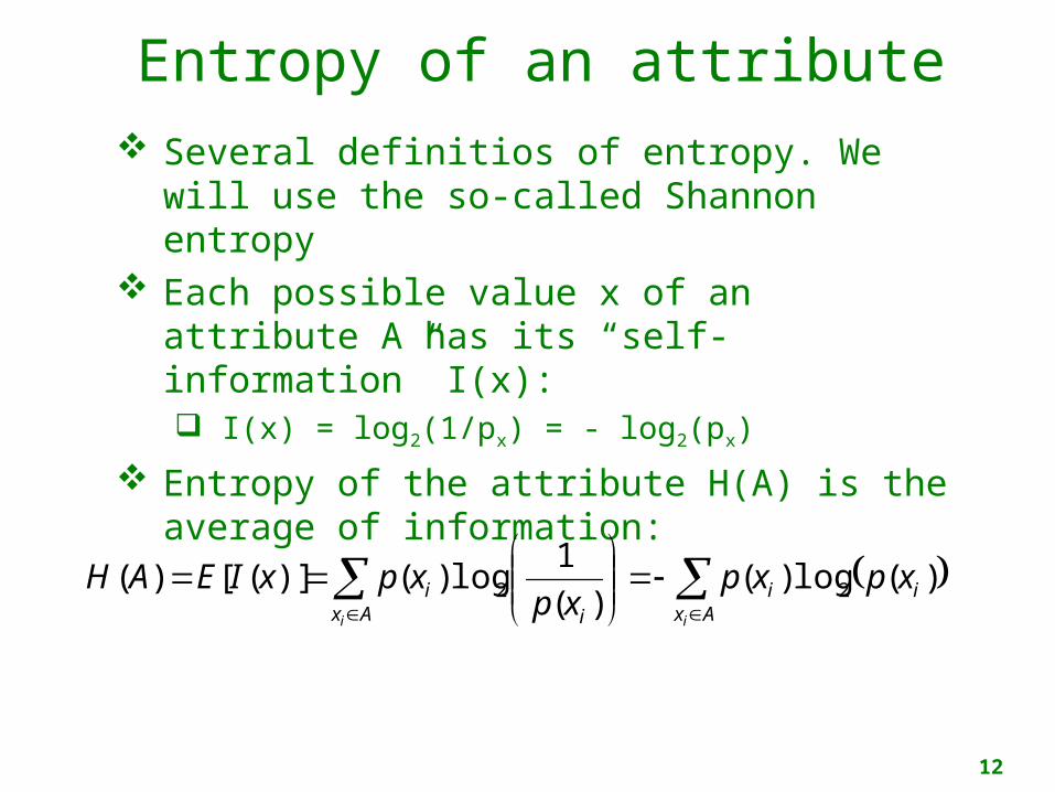
Entropy of an attribute Several definitios of entropy. We will

use the so-called Shannon entropy Each possible value x of an attribute

A has its “self-information” I(x): I(x) = log2(1/px) = - log2(px)

Entropy of the attribute H(A) is the average of information:

Axii

Ax ii

ii

xpxpxp

xpxIEAH )(log)()(

1log)()]([)( 22

13

Claude Shannon, who has died aged 84, perhaps more than anyone laid the groundwork for today’s digital revolution. His exposition of information theory, stating that all information could be represented mathematically as a succession of noughts and ones, facilitated the digital manipulation of data without which today’s information society would be unthinkable.

Shannon’s master’s thesis, obtained in 1940 at MIT, demonstrated that problem solving could be achieved by manipulating the symbols 0 and 1 in a process that could be carried out automatically with electrical circuitry. That dissertation has been hailed as one of the most significant master’s theses of the 20th century. Eight years later, Shannon published another landmark paper, A Mathematical Theory of Communication, generally taken as his most important scientific contribution.

Claude ShannonBorn: 30 April 1916Died: 23 February 2001

“Father of information theory”

Shannon applied the same radical approach to cryptography research, in which he later became a consultant to the US government.

Many of Shannon’s pioneering insights were developed before they could be applied in practical form. He was truly a remarkable man, yet unknown to most of the world.

14

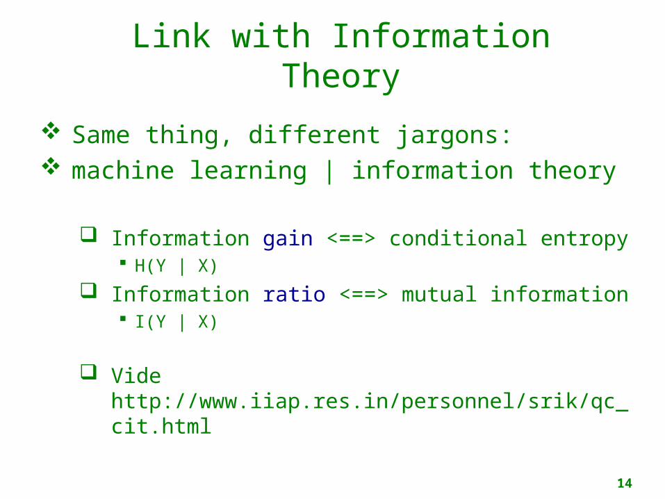
Link with Information Theory

Same thing, different jargons: machine learning | information theory

Information gain <==> conditional entropy H(Y | X)

Information ratio <==> mutual information I(Y | X)

Vide http://www.iiap.res.in/personnel/srik/qc_cit.html

15

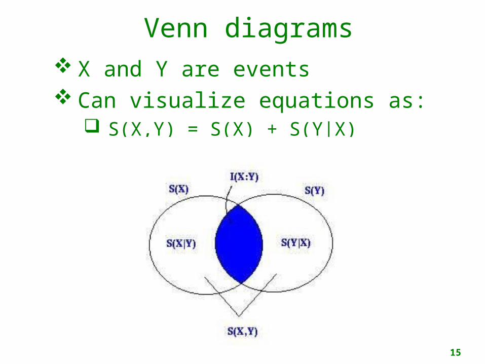
Venn diagrams X and Y are events Can visualize equations as:

S(X,Y) = S(X) + S(Y|X)

16

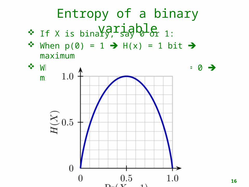
Entropy of a binary variable If X is binary, say 0 or 1: When p(0) = 1 H(x) = 1 bit maximum When p(0)=1 or p(1)=1 H(x) = 0

minimum

17

18

Example: attribute Outlook

Outlook = Sunny :

Outlook = Overcast :

Outlook = Rainy :

Expected information for attribute:

bits 971.0)5/3log(5/3)5/2log(5/25,3/5)entropy(2/)info([2,3]

bits 0)0log(0)1log(10)entropy(1,)info([4,0]

bits 971.0)5/2log(5/2)5/3log(5/35,2/5)entropy(3/)info([3,2]

Note: thisis assumed to be 0 by “continuity” arguments

971.0)14/5(0)14/4(971.0)14/5([3,2])[4,0],,info([3,2] bits 693.0

19

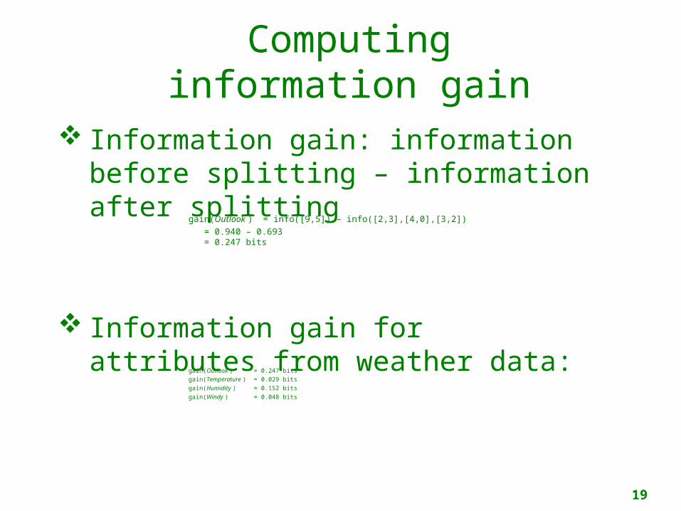
Computinginformation gain

Information gain: information before splitting – information after splitting

Information gain for attributes from weather data:

gain(Outlook ) = 0.247 bitsgain(Temperature ) = 0.029 bitsgain(Humidity ) = 0.152 bitsgain(Windy ) = 0.048 bits

gain(Outlook ) = info([9,5]) – info([2,3],[4,0],[3,2])

= 0.940 – 0.693= 0.247 bits

20

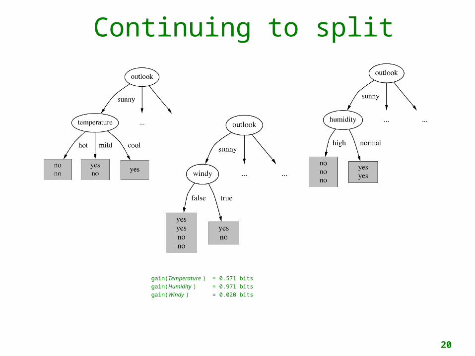
Continuing to split

gain(Temperature ) = 0.571 bitsgain(Humidity ) = 0.971 bitsgain(Windy ) = 0.020 bits

21

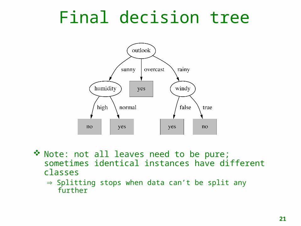
Final decision tree

Note: not all leaves need to be pure; sometimes identical instances have different classes Splitting stops when data can’t be split any further

22

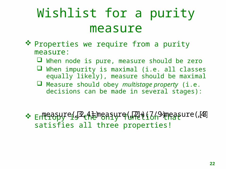
Wishlist for a purity measure

Properties we require from a purity measure: When node is pure, measure should be zero When impurity is maximal (i.e. all classes

equally likely), measure should be maximal Measure should obey multistage property (i.e.

decisions can be made in several stages):

Entropy is the only function that satisfies all three properties!

,4])measure([3(7/9),7])measure([2,3,4])measure([2

23

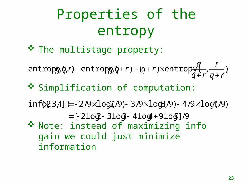
Properties of the entropy

The multistage property:

Simplification of computation:

Note: instead of maximizing info gain we could just minimize information

)entropy()()entropy()entropy(rqr

,rqq

rqrp,qp,q,r

)9/4log(9/4)9/3log(9/3)9/2log(9/2])4,3,2([info 9/]9log94log43log32log2[

24

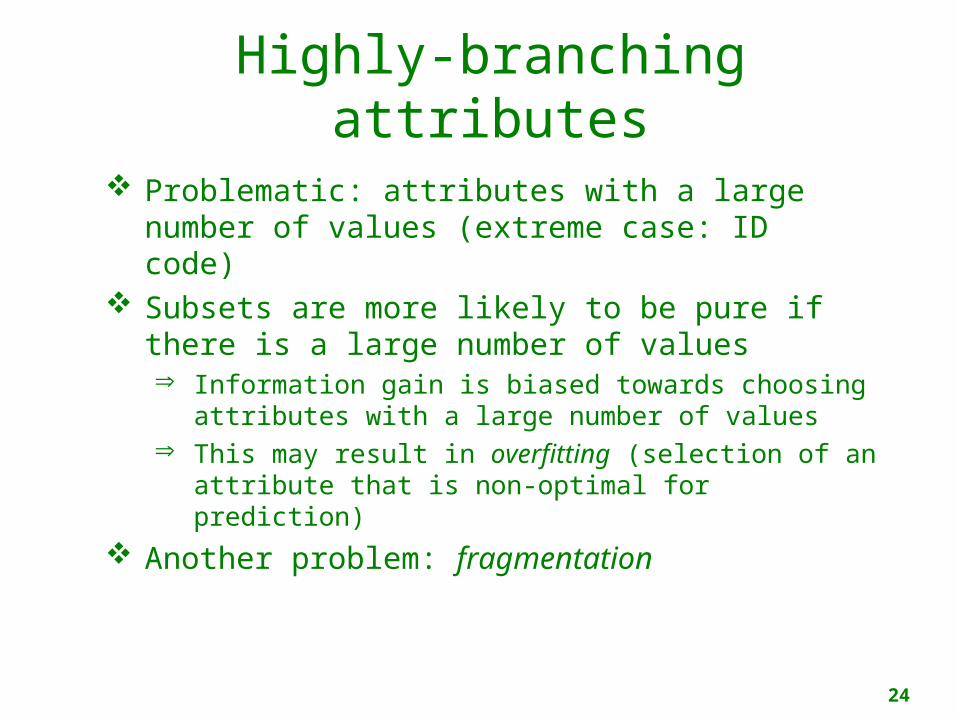
Highly-branching attributes

Problematic: attributes with a large number of values (extreme case: ID code)

Subsets are more likely to be pure if there is a large number of values Information gain is biased towards choosing

attributes with a large number of values This may result in overfitting (selection of an

attribute that is non-optimal for prediction)

Another problem: fragmentation

25

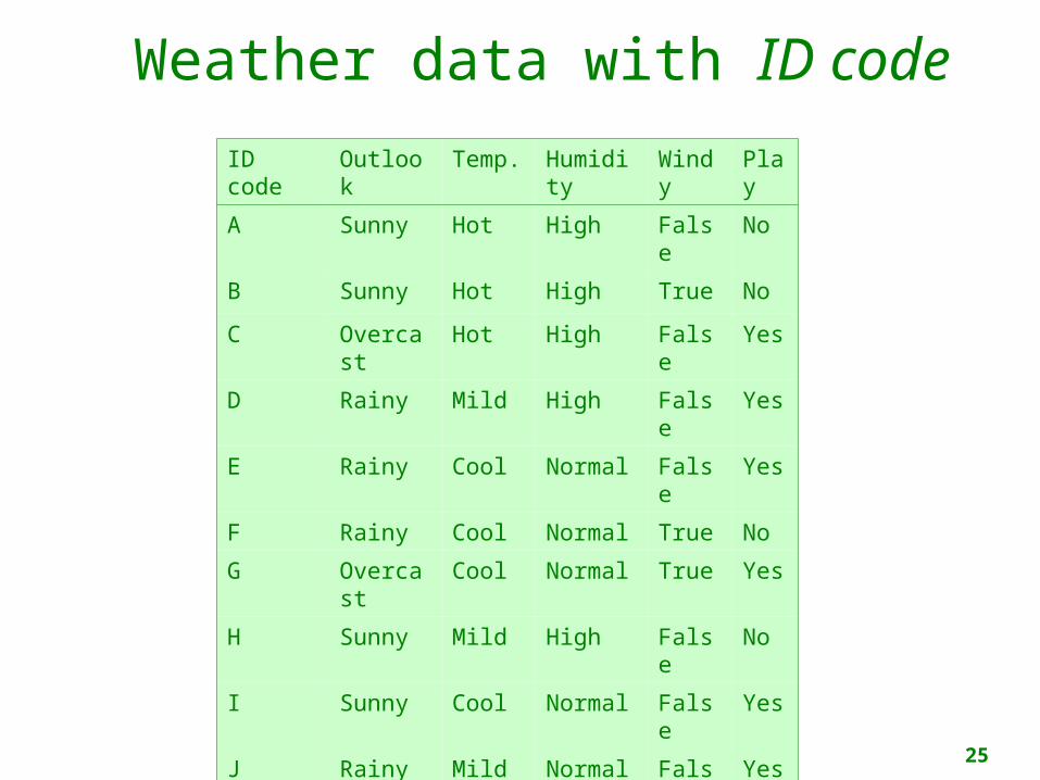
Weather data with ID code

ID code Outlook Temp. Humidity

Windy

Play

A Sunny Hot High False No

B Sunny Hot High True No

C Overcast

Hot High False Yes

D Rainy Mild High False Yes

E Rainy Cool Normal False Yes

F Rainy Cool Normal True No

G Overcast

Cool Normal True Yes

H Sunny Mild High False No

I Sunny Cool Normal False Yes

J Rainy Mild Normal False Yes

K Sunny Mild Normal True Yes

L Overcast

Mild High True Yes

M Overcast

Hot Normal False Yes

N Rainy Mild High True No

26

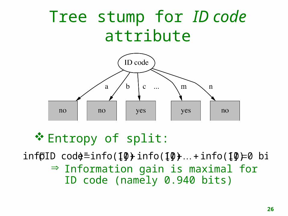
Tree stump for ID code attribute

Entropy of split:

Information gain is maximal for ID code (namely 0.940 bits)

info("ID code") info([0,1]) info([0,1]) info([0,1]) 0 bits

27

Gain ratio

Gain ratio: a modification of the information gain that reduces its bias

Gain ratio takes number and size of branches into account when choosing an attribute It corrects the information gain by taking the

intrinsic information of a split into account Intrinsic information: entropy of

distribution of instances into branches (i.e. how much info do we need to tell which branch an instance belongs to)

28

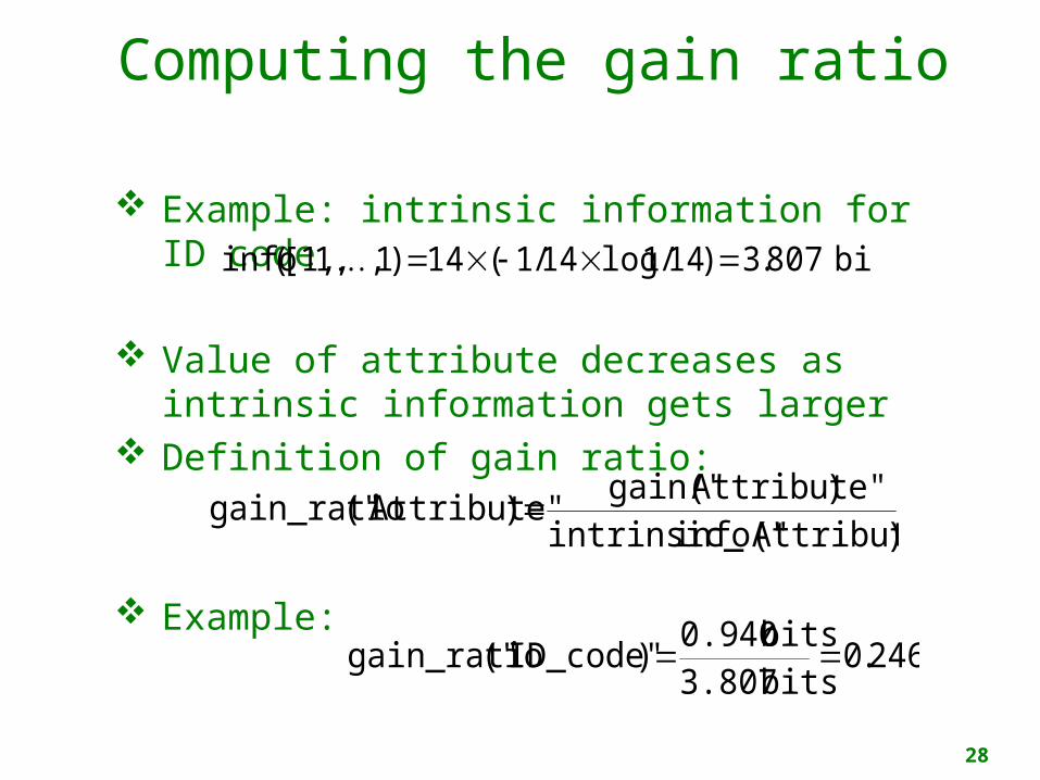
Computing the gain ratio

Example: intrinsic information for ID code

Value of attribute decreases as intrinsic information gets larger

Definition of gain ratio:

Example:

info([1,1,,1) 14 ( 1/14 log1/14) 3.807 bits

)Attribute"info("intrinsic_)Attribute"gain("

)Attribute"("gain_ratio

246.0bits 3.807bits 0.940

)ID_code"("gain_ratio

29

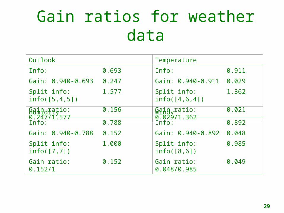
Gain ratios for weather data

Outlook Temperature

Info: 0.693 Info: 0.911

Gain: 0.940-0.693 0.247 Gain: 0.940-0.911 0.029

Split info: info([5,4,5])

1.577 Split info: info([4,6,4])

1.362

Gain ratio: 0.247/1.577

0.156 Gain ratio: 0.029/1.362

0.021Humidity Windy

Info: 0.788 Info: 0.892

Gain: 0.940-0.788 0.152 Gain: 0.940-0.892 0.048

Split info: info([7,7]) 1.000 Split info: info([8,6]) 0.985

Gain ratio: 0.152/1 0.152 Gain ratio: 0.048/0.985

0.049

30

More on the gain ratio

“Outlook” still comes out top However: “ID code” has greater gain

ratio Standard fix: ad hoc test to prevent splitting

on that type of attribute Problem with gain ratio: it may

overcompensate May choose an attribute just because its

intrinsic information is very low Standard fix: only consider attributes with

greater than average information gain

31

Discussion

Top-down induction of decision trees: ID3, algorithm developed by Ross Quinlan Gain ratio just one modification of this basic

algorithm C4.5: deals with numeric attributes,

missing values, noisy data Similar approach: CART There are many other attribute selection

criteria!(But little difference in accuracy of result)