3

1. Introduction

Joan Robinson (1933) developed the idea of monopsonistic discrimination in the labor

market. The idea is simple: a single buyer, a monopsonist, will set wages below marginal

revenue product. The more inelastic labor supply, the lower are wages relative to

productivity. By differentiating wages between groups with different elasticities of labor

supply, the monopsonist may obtain even higher profits. Robinson suggests gender as one

of the dimensions along which the employer may discriminate. If female labor supply is

more inelastic than male labor supply, women will earn less than men relative to their

productivity, and thus face a higher level of exploitation in the labor market.

Modern labor economics does not leave this theory much credit. While Madden

(1973) argues in favor of monopsonistic discrimination, and Ferber, Loeb and Lowry

(1976) and Booton and Lane (1985) find evidence of such behavior in particular labor

markets, the consensus now seems to be that this model does not add much to the

understanding of the overall gender wage gap. This is true on both sides of the Atlantic:

Jane Humphries (1995) writes “But this classic case (pure monopsony) seems to have

little empirical purchase” 1, in the theoretical chapter in The Economics of Equal

Opportunities, edited by herself and Jill Rubury. Blau, Ferber and Winkler (1998) write

in a footnote “It seems likely,..., that the monopsony explanation is more applicable to

specific occupations and specific labor markets than to the aggregate gender pay

differential.” The model is mainly refuted on empirical grounds. Firstly, single buyer

situations are rare, and secondly, female labor supply is found to be at least as elastic as

that of men.

However, recent theoretical developments have revitalized the concept of

monopsony in the labor market. Among the theoretical works, the analyses of job-to-job

flows within a search theoretic framework by Burdett and Mortensen (1998) and

Manning (1994) have established the idea that each single firm or establishment faces its

own individual labor supply curve. The point is that workers quit endogenously, and have

to be replaced by new hires. The higher the wage, the fewer the quits and thus the easier

1 She does, however, add, “women are more constrained than men in choice of employer” and “may facean effective monopsonist, in contrast to men who can travel further and be available more flexibly”. Thispoint is supportive of the view put forward in this paper.

4

it is to attract replacement hires. The idea of an employer-specific supply curve arising

from the dynamics of quits and hires follows the tracks of Hamermesh and Goldfarb

(1970) and Salop (1979), who simply postulate a quit function. In the first section of the

paper, we analyze Robinson’s idea of monopsonistic discrimination within a modern

model framework based on the dynamics of labor supply. We show that given differences

in the exogenous quit rate, in the search effort or in the arrival rate of new jobs for men

and women, a situation with monopsonistic discrimination may occur. We proceed by

analyzing the implications of this model with respect to the wage structure for men and

women in the labor market.

Several conditions have to be met in order for the model of monopsonistic

discrimination to work. One is that it is possible to distinguish between men and women

in the wage setting process. We argue that even in the absence of pure wage

discrimination, - unequal wages for equal work -, it is possible to distinguish between

jobs with uneven gender composition (gender segregation). We present some evidence in

support of this idea. Next, the labor supply curve of women has to be less elastic than the

labor supply curve of men. This is the very point on which the model of monopsonistic

discrimination has been scrapped. It seems that female labor supply is equally, or even

more, wage sensitive than men’s labor supply. However, this point applies largely to the

aggregate labor supply of women, while our concern is the labor supply facing each

employer when considering also job-to-job mobility. The main empirical contribution of

this paper is to estimate a gender-specific relationship between wages and turnover at the

establishment level, thus providing empirical support for the notion that the labor supply

of women facing each employer is less elastic than that of the supply of men. To our

knowledge, this paper is the first serious attempt to estimate gender-specific elasticities of

labor supply facing each establishment.

The recent availability of matched employer-employee data has enabled us to

study the structure of wages and the dynamics of labor markets in greater detail. The

works of Davis, Haltiwanger and Schuh (1996), Lane, Isaac and Stevens (1996) and

Albæk and Sørensen (1998) have established concepts and measures of labor market

flows. Barth and Dale-Olsen (1999b) decomposes the worker flows within and between

employers by gender. With respect to the wage structure, Groshen (1991) and Barth and

5

Mastekaasa (1996) utilize matched employer-employee data to distinguish between wage

effects arising within and between firms. We add to this literature by decomposing the

wage gap within and between establishments and occupations in our data. We are

furthermore able to analyze the relationship between the establishment-specific wage

premium offered to men and the wage premium offered to women2.

Leonard and Audenrode (1996), and Barth and Dale-Olsen (1999a) and Barth and

Schøne (1999) analyze worker flows through establishments and the wage structure

jointly. These papers find support of the notion that the firms wage policy affects the flow

of workers through the firm. Using a 10 percent sample of all Norwegian wage earners,

we are able to study the flow of men and women through the establishments in

considerable detail in this paper. The analysis reveals differences in the establishment-

specific turnover patterns between men and women.

The paper is structured as follows. Chapter 2 presents a theoretical analysis of

monopsonistic discrimination, while chapter 3 discusses some empirical conditions for

the model to make sense. Chapter 4 describes the data. In chapter 5 we analyze wage

differentials between men and women, as well as the establishment-specific wage

premium for each gender. Chapter 6 reports results from turnover and separation

regressions for employers, both for all workers and separately for each gender. Chapter 7

concludes the paper.

2 We use the terms employer and establishment interchangeably throughout. In the empirical analysis, anestablishment is defined by a unique employer and location identification.

6

2. A theory of monopsonistic discrimination

In this section we develop a model of monopsonistic discrimination based on the standard

models of job-to-job search and equilibrium wage distribution of the Burdett and

Mortensen (1998) and Manning (1994) type. Firstly, we go through a stylized model of

labor market frictions, and develop a model of monopsonistic discrimination. Secondly,

we discuss the correlation between the wage policy towards men and women of each

employer. Finally, we briefly discuss issues related to profit equalization across firms and

the number of firms offering jobs to men and women.

The stylized model of labor supply

Assuming that there are some frictions in the labor market, the number of employees the

employer may hire in a given period of time is an increasing function of the wage H (w),

H’ (w) > 0. Furthermore, the fraction of the employer’s stock of employees that leaves

the firm over the same period, is a decreasing function of the wage q (w), q’ (w) < 0. The

following equation then describes the dynamics of the labor force of the employer:

Where Lt is the number of employees at time t. The assumption that quits are

proportional to the number of employees arises from multiplying the individual

separation probabilities. The assumption that the number of hires is a function of w and

independent of L, arises from an assumption of random matching: An employer who puts

one job on the market is assumed to have equal probability of obtaining a match as one

who puts two jobs on the market. See Burdett and Vishwanath (1988) for a discussion.

In steady state, L is constant and the labor supply to any one firm is given by:

We now describe the quit and hiring functions in more detail. Let λ be the probability

that an employee receives a job offer from the wage distribution F (w). δ is an exogenous

separation rate. The probability that an employee separates is then given by q (w) =

1)

2) )()(

)(wq

wHwL =

,L)w(q)w(HLL tt1t −=−+

7

δ+λ(1-F (w)). Consider next the hiring function. Let the probability that an unemployed

worker receives a wage offer be λ as well. We have F (b)=0, where b is the reservation

wage of the unemployed workers. Unemployed workers who receive a wage offer accept.

In addition, the firm hires from employed workers who earn less than w. The distribution

of workers over wages is given by G (w), and may deviate from the distribution of firms

over wages because the number of workers per firm may differ. The hiring function is

then given by:

Where U is the number of unemployed workers, N is the labor force and M is the number

of firms in the economy. The first term is the number of workers hired out of

unemployment while the second term is the number of workers with lower w, hired from

other firms. Consider next the conditions for a stable wage distribution. The number of

new persons entering the labor market at wages less than w is given by λUF (w). At the

same time, qG (w)(N-U) are leaving this tail of the wage distribution because of

exogenous separations or quits into better paying jobs. In steady state, the flow out of

unemployment, λU equals the flow into unemployment δ(N-U). This means that the

steady state unemployment rate is given by δ/(δ+λ) or 1/1+α, where α=λ/δ is a measure

of labor market frictions.

Equating the flows in and out of the wage distribution, and using the condition of

a steady state unemployment rate, we obtain the following relationship between the two

distributions in equilibrium: G (w) = δ F (w) / q (w). Inserting this condition, as well as

the steady state unemployment rate into the hiring function, gives H (w)=λδ/q (w). The

labor supply of each firm is then given by:

This holds in steady state regardless of the shape of the wage distribution (as long as the

employer is constrained to hire according to the hiring function). Burdett and Mortensen

(1998) show that in a profit-maximizing world, F (w) will be continuous and bounded.

With free entry, any employer must earn a profit π=(p-w) L (w) equal to an employer

3)

4) M

N

wFM

N

wqwL

22 )](1([)()(

−+==

λδδλδλ

,M

)UN()w(G

MU

)w(H−

λ+λ=

8

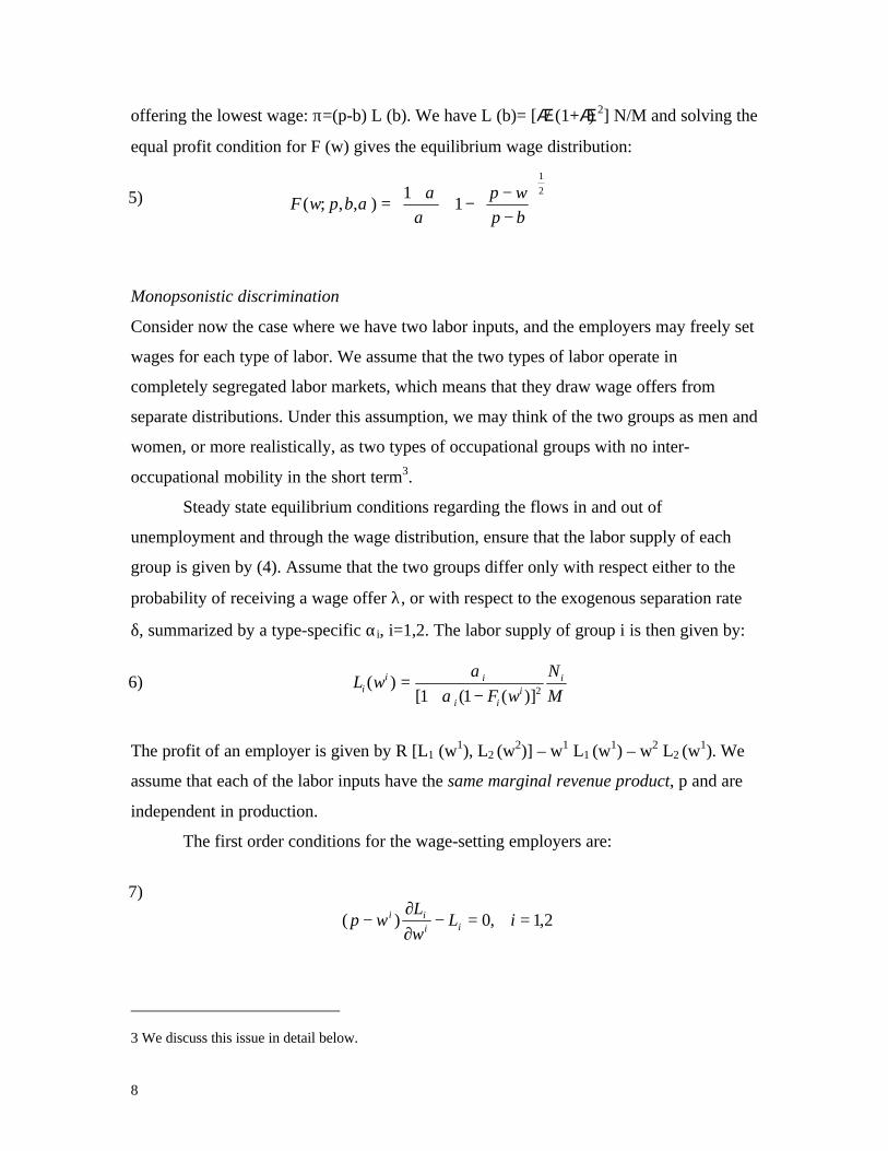
offering the lowest wage: π=(p-b) L (b). We have L (b)= [á/ (1+á) 2] N/M and solving the

equal profit condition for F (w) gives the equilibrium wage distribution:

Monopsonistic discrimination

Consider now the case where we have two labor inputs, and the employers may freely set

wages for each type of labor. We assume that the two types of labor operate in

completely segregated labor markets, which means that they draw wage offers from

separate distributions. Under this assumption, we may think of the two groups as men and

women, or more realistically, as two types of occupational groups with no inter-

occupational mobility in the short term3.

Steady state equilibrium conditions regarding the flows in and out of

unemployment and through the wage distribution, ensure that the labor supply of each

group is given by (4). Assume that the two groups differ only with respect either to the

probability of receiving a wage offer λ, or with respect to the exogenous separation rate

δ, summarized by a type-specific αi, i=1,2. The labor supply of group i is then given by:

The profit of an employer is given by R [L1 (w1), L2 (w

2)] – w1 L1 (w1) – w2 L2 (w

1). We

assume that each of the labor inputs have the same marginal revenue product, p and are

independent in production.

The first order conditions for the wage-setting employers are:

3 We discuss this issue in detail below.

5)

6)

7)

−−

−

+

=2

1

11

),,;(bp

wpbpwF

αα

α

M

N

wFwL i

iii

iii 2)](1(1[

)(−+

=α

α

2,1,0)( ==−∂∂

− iLw

Lwp ii

ii

9

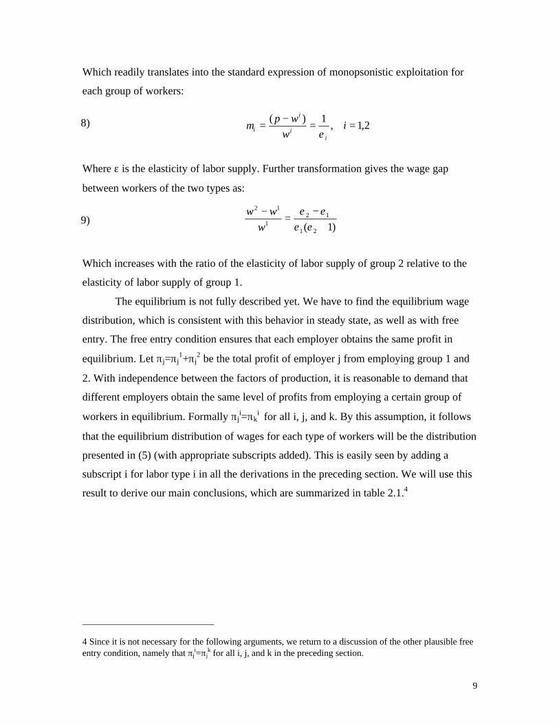
Which readily translates into the standard expression of monopsonistic exploitation for

each group of workers:

Where ε is the elasticity of labor supply. Further transformation gives the wage gap

between workers of the two types as:

Which increases with the ratio of the elasticity of labor supply of group 2 relative to the

elasticity of labor supply of group 1.

The equilibrium is not fully described yet. We have to find the equilibrium wage

distribution, which is consistent with this behavior in steady state, as well as with free

entry. The free entry condition ensures that each employer obtains the same profit in

equilibrium. Let πj=πj1+πj

2 be the total profit of employer j from employing group 1 and

2. With independence between the factors of production, it is reasonable to demand that

different employers obtain the same level of profits from employing a certain group of

workers in equilibrium. Formally πji=πk

i for all i, j, and k. By this assumption, it follows

that the equilibrium distribution of wages for each type of workers will be the distribution

presented in (5) (with appropriate subscripts added). This is easily seen by adding a

subscript i for labor type i in all the derivations in the preceding section. We will use this

result to derive our main conclusions, which are summarized in table 2.1.4

4 Since it is not necessary for the following arguments, we return to a discussion of the other plausible freeentry condition, namely that πj

i=πjk for all i, j, and k in the preceding section.

8)

9)

2,1,1)(

==−

= iw

wp

ii

i

i εµ

)1( 21

121

12

+−

=−

εεεε

w

ww

10

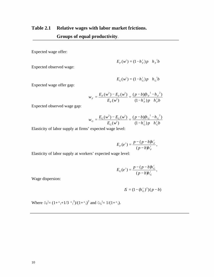
Table 2.1 Relative wages with labor market frictions.

Groups of equal productivity.

Expected wage offer:

Expected observed wage:

Expected wage offer gap:

Expected observed wage gap:

Elasticity of labor supply at firms’ expected wage level:

Elasticity of labor supply at workers’ expected wage level:

Wage dispersion:

Where 0Fi= (1+"i+1/3 "i

2)/(1+"i)2 and 0G

i= 1/(1+"i).

bpwE iF

iF

iF ηη +−= )1()(

bpwE iG

iG

iG ηη +−= )1()(

bp

bp

wE

wEwE

GG

GG

G

GGG 11

21

1

12

)1())((

)()()(

ηηηη

ω+−−−

=−

=

bp

bp

wE

wEwE

FF

FF

F

FFF 11

21

1

12

)1())((

)()()(

ηηηη

ω+−−−

=−

=

)())(1( 2 bpiG

i −−=∆ η

,)(

)()(

iF

iFi

F bp

bppE

ηη

ε−

−−=

,)(

)()(

iG

iGi

G bp

bppE

ηη

ε−

−−=

11

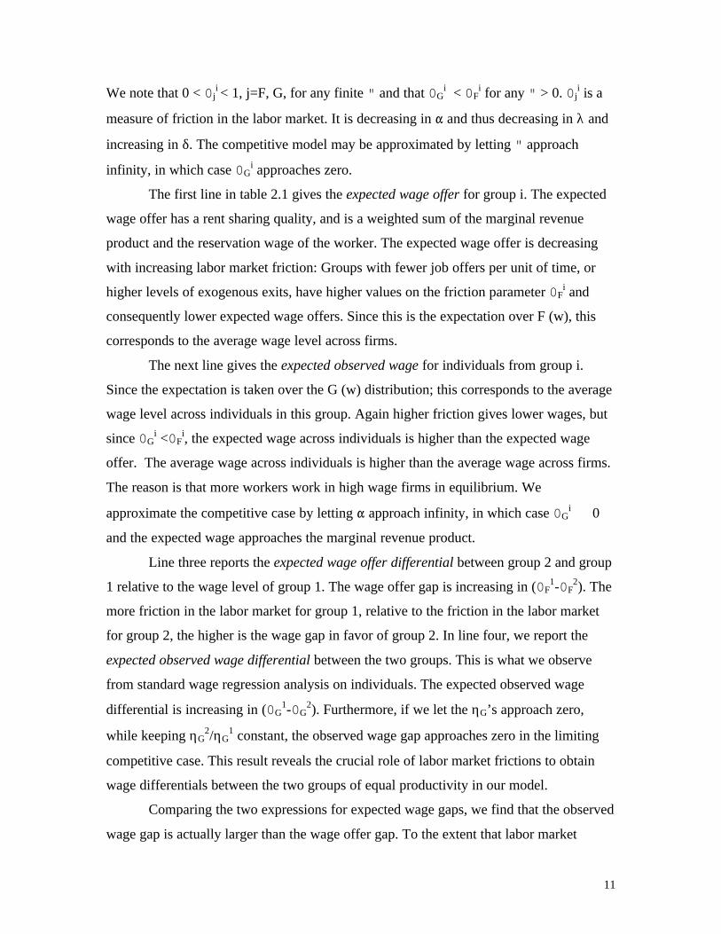
We note that 0 < 0ji < 1, j=F, G, for any finite " and that 0G

i < 0Fi for any " > 0. 0j

i is a

measure of friction in the labor market. It is decreasing in " and thus decreasing in λ and

increasing in δ. The competitive model may be approximated by letting " approach

infinity, in which case 0Gi approaches zero.

The first line in table 2.1 gives the expected wage offer for group i. The expected

wage offer has a rent sharing quality, and is a weighted sum of the marginal revenue

product and the reservation wage of the worker. The expected wage offer is decreasing

with increasing labor market friction: Groups with fewer job offers per unit of time, or

higher levels of exogenous exits, have higher values on the friction parameter 0Fi and

consequently lower expected wage offers. Since this is the expectation over F (w), this

corresponds to the average wage level across firms.

The next line gives the expected observed wage for individuals from group i.

Since the expectation is taken over the G (w) distribution; this corresponds to the average

wage level across individuals in this group. Again higher friction gives lower wages, but

since 0Gi <0F

i, the expected wage across individuals is higher than the expected wage

offer. The average wage across individuals is higher than the average wage across firms.

The reason is that more workers work in high wage firms in equilibrium. We

approximate the competitive case by letting " approach infinity, in which case 0Gi � 0

and the expected wage approaches the marginal revenue product.

Line three reports the expected wage offer differential between group 2 and group

1 relative to the wage level of group 1. The wage offer gap is increasing in (0F1-0F

2). The

more friction in the labor market for group 1, relative to the friction in the labor market

for group 2, the higher is the wage gap in favor of group 2. In line four, we report the

expected observed wage differential between the two groups. This is what we observe

from standard wage regression analysis on individuals. The expected observed wage

differential is increasing in (0G1-0G

2). Furthermore, if we let the ηG’s approach zero,

while keeping ηG2/ηG

1 constant, the observed wage gap approaches zero in the limiting

competitive case. This result reveals the crucial role of labor market frictions to obtain

wage differentials between the two groups of equal productivity in our model.

Comparing the two expressions for expected wage gaps, we find that the observed

wage gap is actually larger than the wage offer gap. To the extent that labor market

12

discrimination should be measured in terms of the wage offer distribution, this result

indicates that the wage gap observed in standard regression studies tends to overestimate

the level of wage discrimination in the labor market. The intuition behind this result is

that, since men work to a higher degree in large high-paying establishments, large

establishments are counted more times for men in the calculation of the observed wage

gap, while in the calculation of the wage offer gap every establishment should be counted

only once.

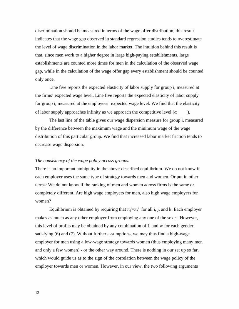
Line five reports the expected elasticity of labor supply for group i, measured at

the firms’ expected wage level. Line five reports the expected elasticity of labor supply

for group i, measured at the employees’ expected wage level. We find that the elasticity

of labor supply approaches infinity as we approach the competitive level ("� �).

The last line of the table gives our wage dispersion measure for group i, measured

by the difference between the maximum wage and the minimum wage of the wage

distribution of this particular group. We find that increased labor market friction tends to

decrease wage dispersion.

The consistency of the wage policy across groups.

There is an important ambiguity in the above-described equilibrium. We do not know if

each employer uses the same type of strategy towards men and women. Or put in other

terms: We do not know if the ranking of men and women across firms is the same or

completely different. Are high wage employers for men, also high wage employers for

women?

Equilibrium is obtained by requiring that πji=πk

i for all i, j, and k. Each employer

makes as much as any other employer from employing any one of the sexes. However,

this level of profits may be obtained by any combination of L and w for each gender

satisfying (6) and (7). Without further assumptions, we may thus find a high-wage

employer for men using a low-wage strategy towards women (thus employing many men

and only a few women) - or the other way around. There is nothing in our set up so far,

which would guide us as to the sign of the correlation between the wage policy of the

employer towards men or women. However, in our view, the two following arguments

13

strongly suggest that the wage policy of the employer will be positively correlated across

groups.

The first argument is based on the fact that if the (common) productivity of

employees differs between employers, the wage distribution of workers will be ranked

according to the productivity ranking of employers. The second argument is based on a

notion of fairness, arguing that relative wages across firms should be consistent between

groups.

We now proceed to show that when employers differ with respect to productivity,

the ranking of male and female wages between the productivity types will be identical.

The discussion draws on the analysis in Burdett and Mortensen (1998) who show, in the

context of one type of labor input only, that the wage and productivity structure will be

correlated in equilibrium.

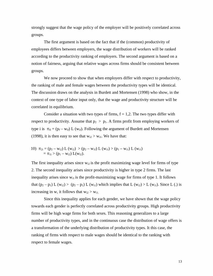
Consider a situation with two types of firms, f = 1,2. The two types differ with

respect to productivity. Assume that p2 > p1. A firms profit from employing workers of

type i is Bfi = (pf – wif) L (wif). Following the argument of Burdett and Mortensen

(1998), it is then easy to see that wi2 > wi1. We have that:

The first inequality arises since wi2 is the profit maximizing wage level for firms of type

2. The second inequality arises since productivity is higher in type 2 firms. The last

inequality arises since wi1 is the profit-maximizing wage for firms of type 1. It follows

that (p2 – p1) L (wi2) > (p2 – p1) L (wi1) which implies that L (wi2) > L (wi1). Since L (.) is

increasing in w, it follows that wi2 > wi1.

Since this inequality applies for each gender, we have shown that the wage policy

towards each gender is perfectly correlated across productivity groups. High productivity

firms will be high wage firms for both sexes. This reasoning generalizes to a large

number of productivity types, and in the continuous case the distribution of wage offers is

a transformation of the underlying distribution of productivity types. It this case, the

ranking of firms with respect to male wages should be identical to the ranking with

respect to female wages.

10) B2i = (p2 – wi2) L (wi2) > (p2 – w1f) L (wi1) > (p1 – wi1) L (wi1) = B1i > (p1 – wi2) L(wi2).

14

Another line of argument is based on internal fairness considerations. It seems

reasonable to assume that firms would adopt a consistent wage policy towards each type

of labor rather than the opposite, simply to reduce internal stress from perceived

differential treatment.

Obviously, there may be factors working in the opposite direction. In particular,

differences in productivity, differences in productivity ranking between firms and a more

complicated technical relationship between the two groups of workers than what is

adopted here could produce rather different results. Consider for instance the (unlikely)

case where the productivity ranking of female jobs is negatively correlated with the

productivity ranking of male jobs, in which case a negative correlation between the wage

premiums of males and females would arise. Our claim here is thus not that wage policies

across groups have to be positively correlated. We only claim that wage differentials

arising from common factors tend to induce similar ranking across firms, and that equity

considerations only strengthens this case. In the end it is an empirical question. We first

produce some evidence below, which goes in the direction of a positive correlation

between the wage policies towards males and females. We then focus on expected wages

in the rest of the paper.

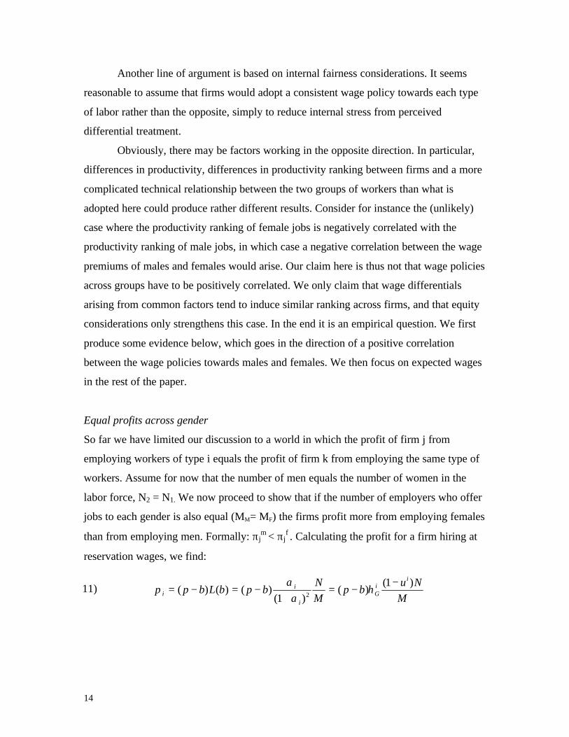
Equal profits across gender

So far we have limited our discussion to a world in which the profit of firm j from

employing workers of type i equals the profit of firm k from employing the same type of

workers. Assume for now that the number of men equals the number of women in the

labor force, N2 = N1. We now proceed to show that if the number of employers who offer

jobs to each gender is also equal (MM= MF) the firms profit more from employing females

than from employing men. Formally: πjm < πj

f . Calculating the profit for a firm hiring at

reservation wages, we find:

11) M

Nubp

M

NbpbLbp

iiG

i

ii

)1()(

)1()()()(

2

−−=

+−=−= η

αα

π

15

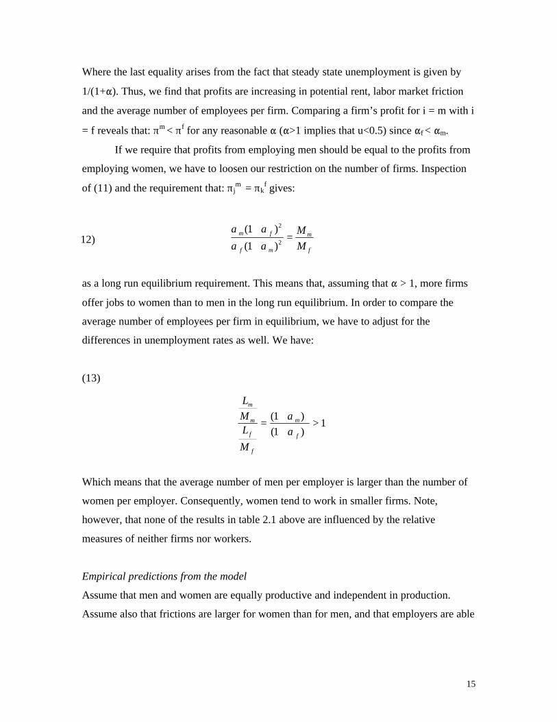
Where the last equality arises from the fact that steady state unemployment is given by

1/(1+"). Thus, we find that profits are increasing in potential rent, labor market friction

and the average number of employees per firm. Comparing a firm’s profit for i = m with i

= f reveals that: πm < πf for any reasonable " (">1 implies that u<0.5) since "f < "m.

If we require that profits from employing men should be equal to the profits from

employing women, we have to loosen our restriction on the number of firms. Inspection

of (11) and the requirement that: πjm = πk

f gives:

as a long run equilibrium requirement. This means that, assuming that " > 1, more firms

offer jobs to women than to men in the long run equilibrium. In order to compare the

average number of employees per firm in equilibrium, we have to adjust for the

differences in unemployment rates as well. We have:

(13)

Which means that the average number of men per employer is larger than the number of

women per employer. Consequently, women tend to work in smaller firms. Note,

however, that none of the results in table 2.1 above are influenced by the relative

measures of neither firms nor workers.

Empirical predictions from the model

Assume that men and women are equally productive and independent in production.

Assume also that frictions are larger for women than for men, and that employers are able

12) f

m

mf

fm

M

M=

+

+2

2

)1(

)1(

αα

αα

1)1()1(

>++

=f

m

f

f

m

m

M

LM

L

αα

16

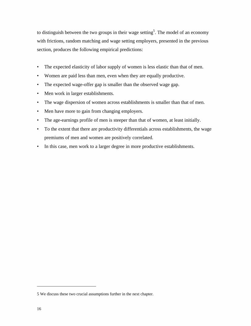
to distinguish between the two groups in their wage setting5. The model of an economy

with frictions, random matching and wage setting employers, presented in the previous

section, produces the following empirical predictions:

• The expected elasticity of labor supply of women is less elastic than that of men.

• Women are paid less than men, even when they are equally productive.

• The expected wage-offer gap is smaller than the observed wage gap.

• Men work in larger establishments.

• The wage dispersion of women across establishments is smaller than that of men.

• Men have more to gain from changing employers.

• The age-earnings profile of men is steeper than that of women, at least initially.

• To the extent that there are productivity differentials across establishments, the wage

premiums of men and women are positively correlated.

• In this case, men work to a larger degree in more productive establishments.

5 We discuss these two crucial assumptions further in the next chapter.

17

3. Gender and the monopsony model

It remains to argue that the model in the preceding chapter is relevant for gender issues.

Basically, such relevance requires that a) the level of labor market friction is higher for

women than for men, and b) that employers may distinguish between men and women in

their wage setting. The empirical part of this paper produces evidence in favor of both

these conditions. In this chapter we discuss these issues more broadly and take a brief

look at some previous evidence.

Do employers distinguish between men and women in their wage setting?

In most advanced industrial countries, there are laws against wage discrimination. Thus,

it seems reasonable to assume that “pure” wage discrimination: “Different pay for the

same job in the same company” is not particularly prevalent. Indeed, all evidence

suggests that the more detailed occupational and institutional controls you include in the

wage equation, the smaller is the observed wage gap (Blau 1974; Petersen and Morgan

1995; Groshen 1991; Barth and Mastekaasa 1996; Barth and Yin, 1996). However, it is

important to note that this exercise may be driven into the absurd by controlling for too

detailed job-titles. Very detailed job-titles often define the wage more or less exactly, and

may be viewed as a “name of the wage” rather than a different occupation. By controlling

for a too detailed job-level, one actually controls for the wage. The assignment of people

to different job-titles gives the employer a possibility of distinguishing between groups of

employees without being in conflict with neither prevailing norms nor with the law.

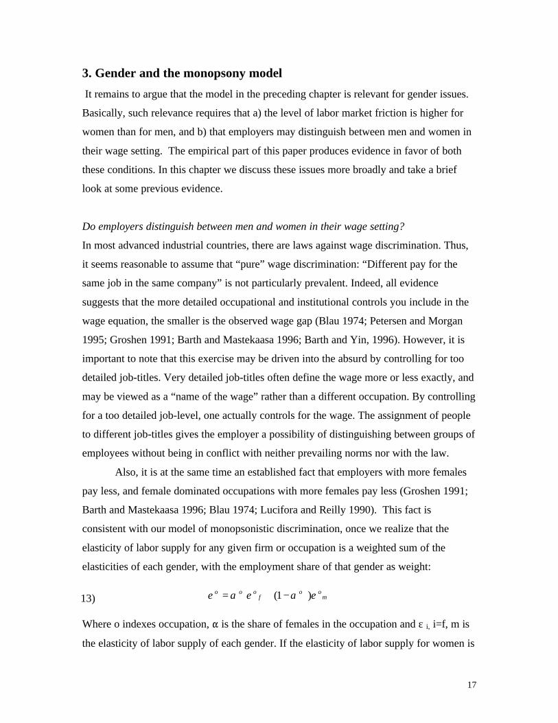
Also, it is at the same time an established fact that employers with more females

pay less, and female dominated occupations with more females pay less (Groshen 1991;

Barth and Mastekaasa 1996; Blau 1974; Lucifora and Reilly 1990). This fact is

consistent with our model of monopsonistic discrimination, once we realize that the

elasticity of labor supply for any given firm or occupation is a weighted sum of the

elasticities of each gender, with the employment share of that gender as weight:

Where o indexes occupation, " is the share of females in the occupation and ε i, i=f, m is

the elasticity of labor supply of each gender. If the elasticity of labor supply for women is

13) moo

fooo εαεαε )1( −+=

18

less elastic than that of men, the elasticity of labor supply of a female dominated

occupation or establishment is less elastic than that of a male dominated occupation or

establishment.

We add below to the evidence showing that employers with more women pay

less, and furthermore that those occupations with more women pay less. This evidence is

clearly consistent with the presented model of monopsonistic wage discrimination.

Differences in turnover between men and women

A large part of the literature on gender and the labor market assumes that the women

have higher turnover than men do. Examples are Goldin (1986), who finds that when

turnover rates differ between the sexes, occupational segregation arises as a result of

different strategies for supervising male and female workers. Polachek (1981) argues that

women choose less human capital investments because of higher expected turnover rates.

Lazear and Rosen (1990) find that differential treatment in promotions will be the

outcome of differences in quit behavior. While these studies find that the differential

treatment of men and women is efficient, the present analysis argues that differences in

turnover leads to monopsonistic discrimination which is not efficient.

There is also a strand of literature that argues that women turnover is actually

similar to that of men’s, once appropriate controls are introduced. Blau and Kahn (1981)

and Galizzi (1999) find that the propensities to quit are similar once differences in wages

or expected wages are appropriately controlled for. Viscusi (1979) argues that “sex

differences in quitting have been overdrawn in many previous discussions.” However,

the results are obtained conditional on tenure. Tenure is found to mean a great deal to the

overall differences in turnover rates. Viscusi (1979) finds that this factor is the most

important single difference between the sexes.

Lynch (1991) finds that the difference between the log of the current wage and a

log predicted wage affects both separations of men and women from their first job in a

sample of young workers who have just left school. The point estimate of the effect of

wages on the probability of leaving the employer is actually larger for women than men.

However, since the sample is restricted to youths in their first job after school, the results

do not necessarily generalize to the labor market as a whole.

19

Evidence of differences in turnover behavior between men and women are found

in several recent studies. Loprest (1992) finds that young women have on average less

than 50 percent of the wage growth of young men when changing jobs. This difference

constitutes the main reason why younger women have lower wage growth than younger

men. Schøne (1998) finds similar results for Norway. Sicherman (1996) finds that, at low

levels of tenure, women have higher rates of departures than men do. Furthermore, the

negative tenure effect on departure is much stronger among women than men. After five

years of tenure, women were less likely than men were to leave the firm. He also finds

that the reasons for quitting are different between men and women. Pissarides and

Wadsworth (1994) conclude from an analysis of job search behavior in the UK, that

women “appear to base their job search decision on factors largely unconnected with the

conditions on labor demand.” Using data from the NLSY in the U.S., Keith and

McWilliams (1998) find that women are much more likely to change jobs for a family-

related reason than are men. Also, men engage in more employed job search than women.

They also find that those who search while employed earn the largest return to mobility.

There are several good reasons why we would expect women’s turnover pattern to

be different than men’s turnover pattern. In particular, we would expect higher labor

market frictions (higher δ and lower λ) for the following reasons:

Fundamental differences:

- Men’s traditional role as a breadwinner. The income effect through their spouses is

dominant in the household. This means that events related to the male’s labor market

condition, e.g. wage raises, promotions, geographical moves, unemployment etc.

affect the women’s choices more strongly than the other way around. This leads to

higher δ.

- Women do more of the work in the household. This means that productivity shocks

(children, illness in the family etc) in the household sphere affects women more

strongly. This also leads to a higher δ.

- Traditional norms may limit the number of jobs available (or attractive) to women,

thus limiting their choices and thus λ.

20

Enforcement mechanisms on both sides of the market:

- If women know they will have higher turnover, they may invest less in the labor

market and choose occupations with lower punishment of turnover. Again reducing λ

- If employers think that women have higher turnover, they may choose to give women

fewer opportunities, lowering λ.

- If employers use the monopsony power to keep wages lower, and wages for women

are less dispersed, women have less incentives to search, thus lowering λ

- Specialization may lead to higher productivity at home, and limited occupational

choices to those that may use those skills. (λ)

All in all there are many good reasons why there may be more friction in the labor market

for women than men. However, note that, as women become more similar to men and

vice versa, in terms of both labor market and home production, all the fundamental

differences are reduced, which eventually will cause the feedback effects to subside as

well.

In section 6 below, we produce some novel evidence of different turnover patterns

between men and women through the establishments. Our results show that the turnover

of women is less elastic with respect to wages than the turnover of men, implying that the

elasticity of labor supply facing each firm is less elastic for women than men.

21

4. Data and worker-flow measures

Our data are based on a sample of more than 17,000 employers and over 200,000

employees. This is a representative 10 percent sample of all jobs in Norway in 1990. Due

to the self-weighting sampling process, large employers are over-sampled. We restrict the

data set to employers who have at least one employee on January 1, 1990 or on January

1, 1991. The data covers the period 1989-1991. We mainly use information from the

register of employees and employer, but also information from register of salaries and

taxation and register of education is used. All registers are a part of an integrated register

based data system (CSSD) linked by Statistics Norway.

We use standard definitions of job and worker flows (see e.g. Burgess, Lane,

Stevens 1996, and Davis, Haltiwanger and Shuh 1996). The stocks of employees are

defined as the number of employees January 1, 1990 (nt-1) and the number of employees

January 1, 1991 (nt). Starts and separations are defined by starts (h) and separations (q)6

during the period of January 2, 1990 to December 31, 1990. For each employer, net job

flow (JF=nt – nt-1) is defined as employment growth during one year. If it is positive, we

have gross job creation (JC= |nt – nt-1| when JF≥0, otherwise JC=0), if it is negative there

is gross job destruction (JD=|nt-nt-1| when JF<0, otherwise JD=0). Gross job flow

(AJF=|nt – nt-1|) is the absolute value of net job flow. When we sum over more than one

establishment, AJF represents gross job reallocation as both job creation and job

destruction enter positively. Worker flow (WF=H + Q) is defined as the sum of hires and

separations during the year. Churning flow (CF=WF – AJF), or excess turnover, is

defined as the part of the worker flow that is not necessary to accommodate the job flow.

Churning flow is thus the part of worker flow that would remain even in a stationary

environment where each firm kept its stock of workers constant. Each of the terms are

made into rates by dividing by the average stock of workers during the year. These rates

are denoted (in the same order as above) JFR, JCR, JDR, AJFR, HR, QR and so on.

The corresponding gender-specific rates are created by evaluating the same

expression for men and women, separately. Decomposing these measures into group-

specific measures of job and worker flows, involve some definitional problems. Net job

22

flow for one group in an establishment may be higher or lower than overall net job flow

within the establishment. Even in a stable firm with zero employment growth, we may

have job creation for one group, with a corresponding level of job destruction for another

group. In this case churning for each group will be less than total churning, since there is

gross job reallocation on the decomposed level, while there is zero job flow on the

aggregate level within the firm. We thus need a measure of the part of the churning which

contributes to a change in the input mix between the groups. We have chosen the

following definitions:

Let AJFj be the gross job flow of group j and κj the employment share of group j.

Then define: Excess gross job flow (AEJFj) (for gender j) as the part of job flow for that

group which deviates from the gross job flow in the firm: AEJFj = AJFj - κjAJF. Excess

gross job flow is zero if job creation or destruction hits the groups proportionally, if not,

excess gross job flow is a measure of the reallocation between groups within firms.

In a similar way, let EJFj be the excess net job flow (for gender j); the job flow of

group i which is in excess to a proportional flow to the establishment’s net job flow: EJFj

= JFj - κjJF. Excess net job flow for gender j may be viewed as measure of the movement

along an isoquant for the establishment, thus inducing a change in the gender ratio of the

establishment. If the establishment employs men and women in the fifty-fifty proportion,

creates 20 jobs of which 15 are male jobs, the excess net job flow for women is -5 while

it is +5 for men. Excess net job flow is thus a measure of the excess job flow for each

group, which cancels to zero for the whole establishment, while excess gross job flow is a

measure of the reallocation of jobs between groups, involving both a substitution effect

and a scale effect.

Defining the churning for each group as the sum of hires and separations minus

gross job flow for this group: CFj= WFj - AJFj, we obtain the following decomposition of

the total churning flow of establishment i:

6 We use the terms “separate” and “separations”, since we do not know whether the employee quitsvoluntarily or if the employee was fired.

14) ,CFCF iji ijAEJFκκ +=

23

Or in terms of rates:

We use both the churning rate and the separation rate as dependent variables in

the establishment-level regression analysis in chapter 6. Our third dependent variable in

chapter 6, adjusted separation rates, are constructed in a slightly more elaborate way:

We define a dummy-variable, S=1 if an employee separates, otherwise S=0. Then

we run separate regressions for each gender, based only on within-establishment

variations in S and covariates (fixed-employer-effect model)7. The covariates are

education, experience, and the interaction between education and experience plus second

order terms. Let Zifα represent the covariates and their coefficients. Let the global

average of Sif and Zif be denoted S and Z . We then calculate the individual’s deviation

from his expected separation probability:

Where pred (S)if is the employees expected separation behavior, defined by the last

equality and withinZSconsta α−= . The residual ρif is normalized by deducting the

average deviation from the expected separation behavior of employees, and thus the

mean of the normalized residual across all individuals equals zero. We estimate the

establishment-specific adjusted separation rate, Πf by:

7 We use a linear probability model because of computational problems involved in estimating a fixed-employer effect probit model.

15)

16)

17)

withinififififif ZconstaSSpredS αρ −−=−=∧

)(

ρ .ff =Π

).(CFRCFR iji ijj AEJFR+= κ

24

5. Male-Female Wage Differentials and the Wage Premium of the

Employers

This section presents results for the male female wage differentials in Norway. First, we

present some figures for the average wage differences between men and women. Next,

we show that wages tend to fall with the share of females, both across occupations and

employers, even after control for human capital and the within-group wage differential

between men and women. The point is to show that even if employers do not differentiate

between men and women within the same job, they may differentiate between jobs and

occupations. The observation of a negative relationship between occupational- and firm-

specific wage levels, even after controlling for individual attributes, is consistent with our

theoretical model presented earlier.

We proceed by estimating the gender–x-employer specific wage premiums to be

used in the turnover analysis later on. Also, we answer the question: Are high wage

employers for men, also high wage employers for women? As we discussed in the

theoretical section, it is not clear from theory what the answer should be to this question.

We did, however, present two arguments in favor of a positive correlation between the

wage premiums of men and women. Firstly, high-rent firms should represent the upper

part of the wage distribution for both sexes. Secondly, wage comparisons within the

establishment are likely to bring about some convergence in the employer’s wage policy

across gender or jobs.

Male-Female Wage Differentials

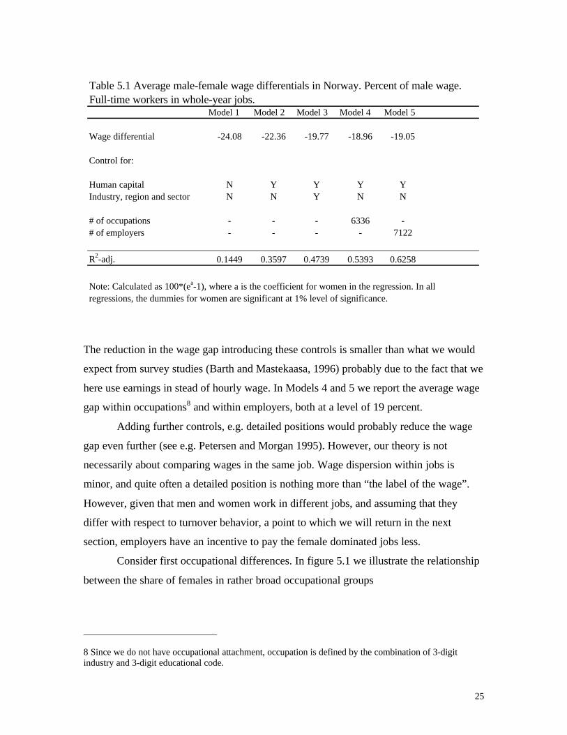
We start out with some introductory calculations of the male-female wage gap. Table 5.1

reports the average male-female wage gap calculated from the gender coefficient of

regression models including different types of controls. The analysis is done for full-time

(30+ hrs)-whole year jobs only. Model 1 gives the raw wage gap of 24 percent. Model 2

controls for years of education, experience, seniority and their squares. The wage gap is

reduced to 22 percent by the introduction of these controls. Model 3 includes 3 digit

industries, sector and region as well, reducing the average wage gap to 20 percent.

25

The reduction in the wage gap introducing these controls is smaller than what we would

expect from survey studies (Barth and Mastekaasa, 1996) probably due to the fact that we

here use earnings in stead of hourly wage. In Models 4 and 5 we report the average wage

gap within occupations8 and within employers, both at a level of 19 percent.

Adding further controls, e.g. detailed positions would probably reduce the wage

gap even further (see e.g. Petersen and Morgan 1995). However, our theory is not

necessarily about comparing wages in the same job. Wage dispersion within jobs is

minor, and quite often a detailed position is nothing more than “the label of the wage”.

However, given that men and women work in different jobs, and assuming that they

differ with respect to turnover behavior, a point to which we will return in the next

section, employers have an incentive to pay the female dominated jobs less.

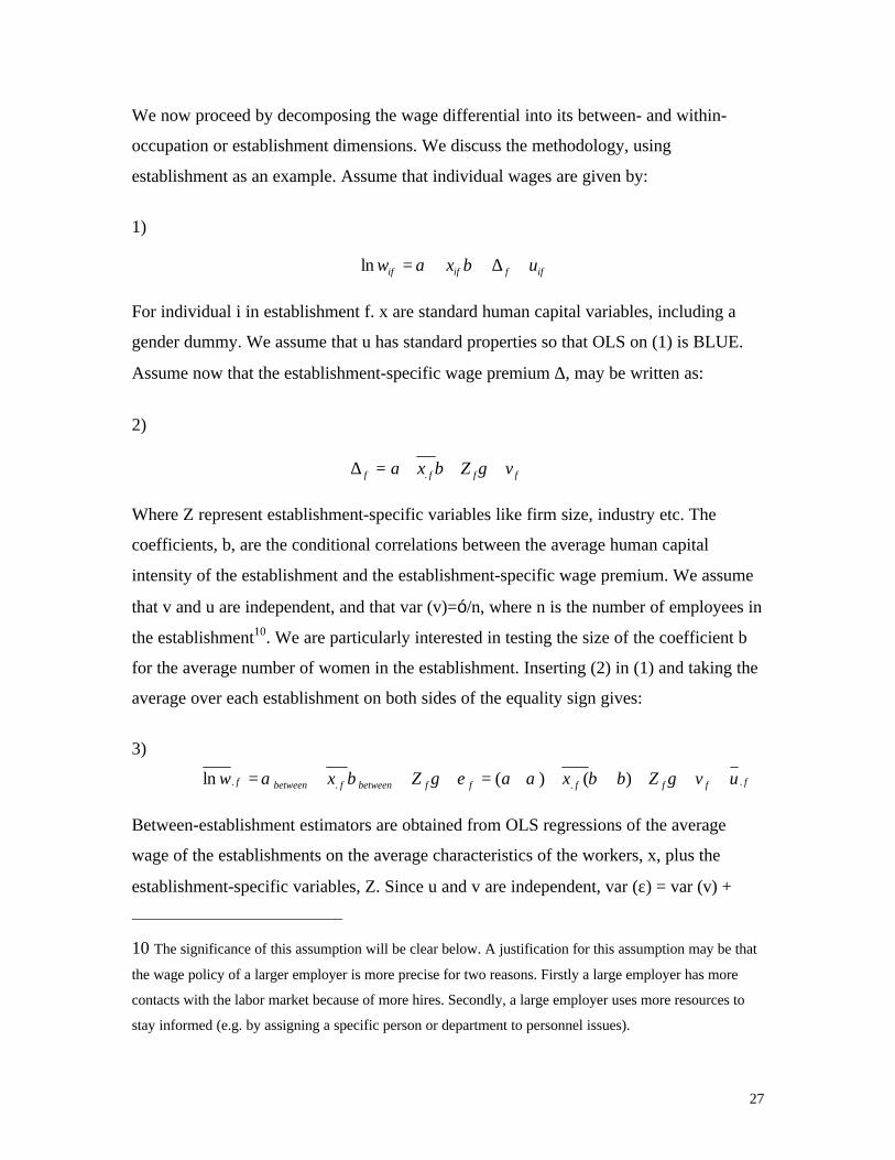
Consider first occupational differences. In figure 5.1 we illustrate the relationship

between the share of females in rather broad occupational groups

8 Since we do not have occupational attachment, occupation is defined by the combination of 3-digitindustry and 3-digit educational code.

Model 1 Model 2 Model 3 Model 4 Model 5

Wage differential -24.08 -22.36 -19.77 -18.96 -19.05

Control for:

Human capital N Y Y Y YIndustry, region and sector N N Y N N

# of occupations - - - 6336 -# of employers - - - - 7122

R2-adj. 0.1449 0.3597 0.4739 0.5393 0.6258

Table 5.1 Average male-female wage differentials in Norway. Percent of male wage. Full-time workers in whole-year jobs.

Note: Calculated as 100*(ea-1), where a is the coefficient for women in the regression. In all regressions, the dummies for women are significant at 1% level of significance.

26

Figure 5.1. Wage premium and the share of women in broad occupations.

Note: Occupations are defined as individuals with identical number of years of education and 3-digit

industry. Wage premiums are calculated as deviations from the employment weighted means of the

coefficients of the occupational dummies in a wage regression also including education, experience,

seniority and their squares as well as a gender dummy. The share of females is calculated from the

observations in the sample.

(Defined as years of educationX3-digit industry) and the wage premium for this

occupation, calculated from a model including human capital controls as model 2 in table

5.1. The model also included a gender dummy for individuals9, which ensures that the

observed relationship is not merely a result of adding up the gender differentials within

occupations.

9 The estimated coefficient for the gender dummy within these broad occupational groups was 19.4percent.

-80

-60

-40

-20

0

20

40

60

80

100

0 10 20 30 40 50 60 70 80 90 100

Share of women in occupation (%)

Wag

e pr

emiu

m in

occ

upat

ion

(%)

27

We now proceed by decomposing the wage differential into its between- and within-

occupation or establishment dimensions. We discuss the methodology, using

establishment as an example. Assume that individual wages are given by:

1)

For individual i in establishment f. x are standard human capital variables, including a

gender dummy. We assume that u has standard properties so that OLS on (1) is BLUE.

Assume now that the establishment-specific wage premium ∆, may be written as:

2)

Where Z represent establishment-specific variables like firm size, industry etc. The

coefficients, b, are the conditional correlations between the average human capital

intensity of the establishment and the establishment-specific wage premium. We assume

that v and u are independent, and that var (v)=ó/n, where n is the number of employees in

the establishment10. We are particularly interested in testing the size of the coefficient b

for the average number of women in the establishment. Inserting (2) in (1) and taking the

average over each establishment on both sides of the equality sign gives:

3)

Between-establishment estimators are obtained from OLS regressions of the average

wage of the establishments on the average characteristics of the workers, x, plus the

establishment-specific variables, Z. Since u and v are independent, var (ε) = var (v) +

10 The significance of this assumption will be clear below. A justification for this assumption may be that

the wage policy of a larger employer is more precise for two reasons. Firstly a large employer has more

contacts with the labor market because of more hires. Secondly, a large employer uses more resources to

stay informed (e.g. by assigning a specific person or department to personnel issues).

iffifif uxw +∆++= βαln

ffff vZbxa +++=∆ γ.

ffffffbetweenfbetweenf uvZbxaZxw .... )()(ln ++++++=+++= γβαεγβα

28

var(u) = (óv+ óu)/n, and thus it is appropriate to weight the between-establishment

regressions with the square root of the number of employees.

From (3) it is clear that we may estimate b as the difference between the between-

establishment estimator (βbetween) and the within-establishment estimator (β):

Since the between- and within-establishment variation in the data is orthogonal, we may

use the formula for the sum of two independent stochastic variables to calculate the

variance of b:

And with normality assumptions, we may use a standard t-test to evaluate the

significance of b.

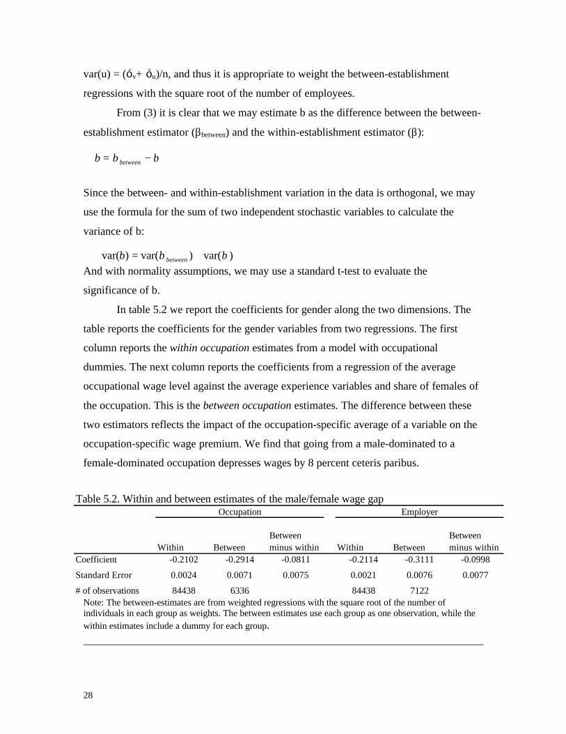
In table 5.2 we report the coefficients for gender along the two dimensions. The

table reports the coefficients for the gender variables from two regressions. The first

column reports the within occupation estimates from a model with occupational

dummies. The next column reports the coefficients from a regression of the average

occupational wage level against the average experience variables and share of females of

the occupation. This is the between occupation estimates. The difference between these

two estimators reflects the impact of the occupation-specific average of a variable on the

occupation-specific wage premium. We find that going from a male-dominated to a

female-dominated occupation depresses wages by 8 percent ceteris paribus.

Note: The between-estimates are from weighted regressions with the square root of the number ofindividuals in each group as weights. The between estimates use each group as one observation, while thewithin estimates include a dummy for each group.

ββ −= betweenb

)var()var()var( ββ += betweenb

Within BetweenBetween minus within Within Between

Between minus within

Coefficient -0.2102 -0.2914 -0.0811 -0.2114 -0.3111 -0.0998

Standard Error 0.0024 0.0071 0.0075 0.0021 0.0076 0.0077

# of observations 84438 6336 84438 7122

Table 5.2. Within and between estimates of the male/female wage gapOccupation Employer

29

The next three columns of table 5.2 report results from a similar exercise for employers.

We find that the between employers estimate of the male-female wage gap is 31 percent.

Of this, 21 percentage points arise within employers while 10 percentage points arise

between employer. Female dominated employers pay less and increasing the share of

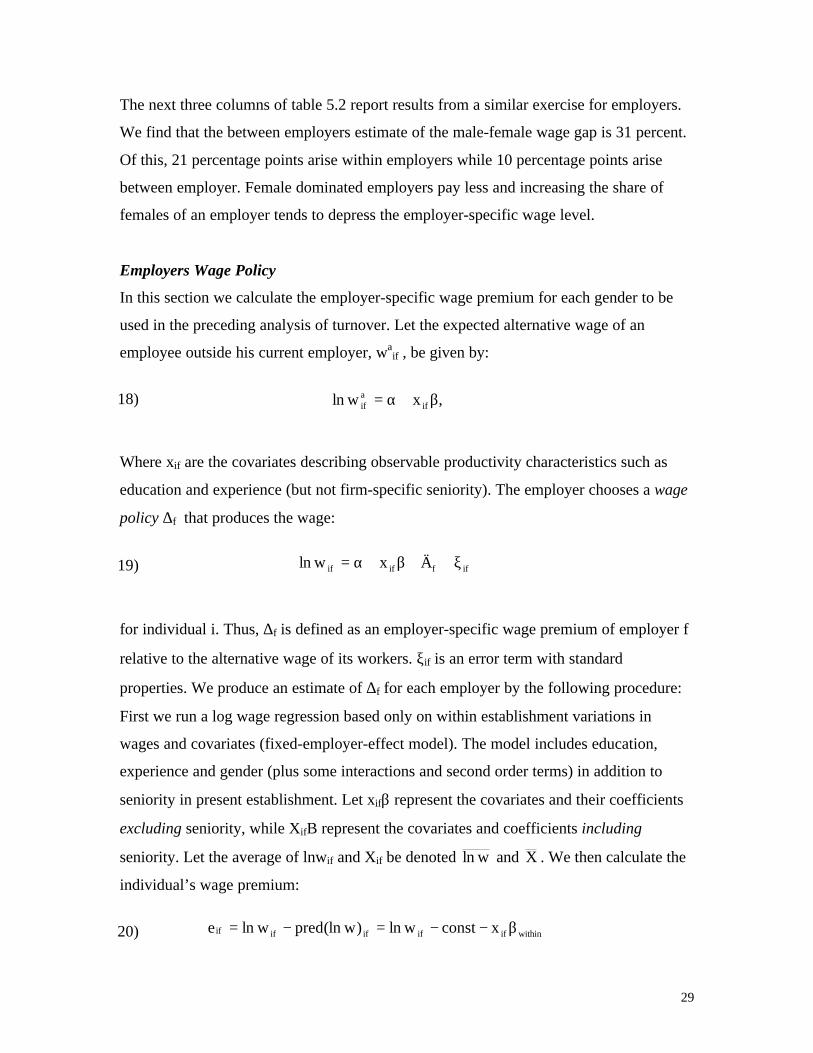
females of an employer tends to depress the employer-specific wage level.

Employers Wage Policy

In this section we calculate the employer-specific wage premium for each gender to be

used in the preceding analysis of turnover. Let the expected alternative wage of an

employee outside his current employer, waif , be given by:

Where xif are the covariates describing observable productivity characteristics such as

education and experience (but not firm-specific seniority). The employer chooses a wage

policy ∆f that produces the wage:

for individual i. Thus, ∆f is defined as an employer-specific wage premium of employer f

relative to the alternative wage of its workers. ξif is an error term with standard

properties. We produce an estimate of ∆f for each employer by the following procedure:

First we run a log wage regression based only on within establishment variations in

wages and covariates (fixed-employer-effect model). The model includes education,

experience and gender (plus some interactions and second order terms) in addition to

seniority in present establishment. Let xifβ represent the covariates and their coefficients

excluding seniority, while XifB represent the covariates and coefficients including

seniority. Let the average of lnwif and Xif be denoted wln and X . We then calculate the

individual’s wage premium:

18)

19)

20)

,xwln ifaif β+α=

iffifif Äxwln ξ++β+α=

withinififififif xconstwln)w(lnpredwlne β−−=−=∧

30

Where pred (lnw)if is the alternative wage defined by the last equality and

withinBXwlnconst −= . Note that since pred (lnw)if does not include the individual’s

return to seniority, the residual eif measures the wage premium including the returns to

seniority. The residual is normalized to be equal to zero for new employees, and the mean

of the residual across all individuals thus measures the average return to seniority. We

estimate ∆f by:

We estimate the wage policy of the employer using a sample of 84,400 wage earners who

satisfy the following two criteria: 1) wage earners who do not change employer during

1990 in establishments with at least two full-time wage earners during 1990. 2) wage

earners who work full-time (30+ hours a week).

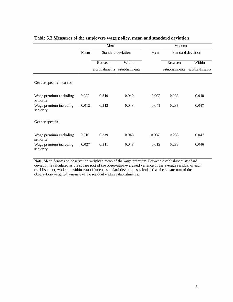
Table 5.3 reports the level and dispersion of several measures of the wage

premium of the employer for each gender. We report figures for both the gender-specific

mean of the wage premium from joint regressions (Gender- specific mean of..) and

figures calculated from separate regressions for men and women (Gender-specific..). For

both groups, the standard deviation of the wage premium is higher between

establishments than within establishments. Note that while women have lower wage

dispersion than men, the difference is more or less entirely due to lower wage dispersion

across employers. The within employers residual wage dispersion is in the range .046-.

049 for both groups. Lower wage dispersion across establishments is exactly what our

theoretical model predicts (see the last line of table 2.1.).

The correlation between the two gender premiums is 42.7 percent and signifi-

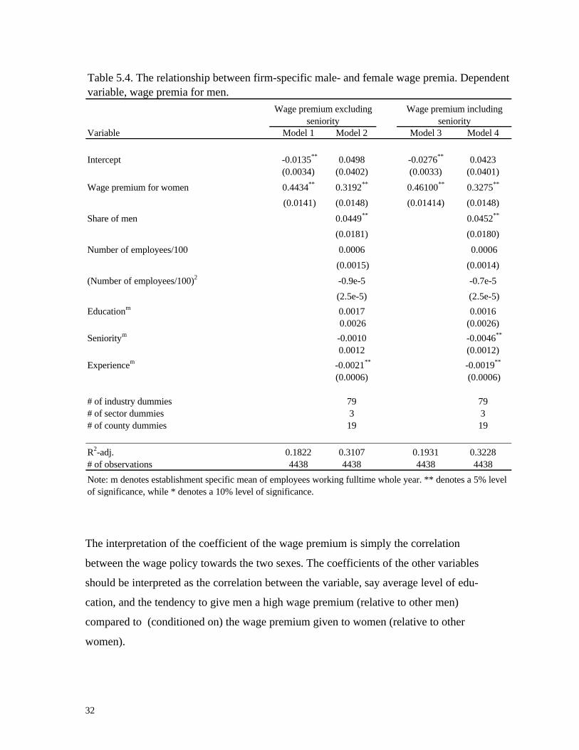
cantly positive. This is what we expected from the theoretical model. In Table 5.4 we

study the relationship between the two wage premiums in some more detail using

regression analysis. We regress the wage premium of men on the wage premium of

women and some other variables.

21) e=Ä̂ .ff

31

Table 5.3 Measures of the employers wage policy, mean and standard deviation

Men Women

Mean Standard deviation Mean Standard deviation

Between

establishments

Within

establishments

Between

establishments

Within

establishments

Gender-specific mean of

Wage premium excludingseniority

0.032 0.340 0.049 -0.002 0.286 0.048

Wage premium includingseniority

-0.012 0.342 0.048 -0.041 0.285 0.047

Gender-specific

Wage premium excludingseniority

0.010 0.339 0.048 0.037 0.288 0.047

Wage premium includingseniority

-0.027 0.341 0.048 -0.013 0.286 0.046

Note: Mean denotes an observation-weighted mean of the wage premium. Between establishment standarddeviation is calculated as the square root of the observation-weighted variance of the average residual of eachestablishment, while the within establishments standard deviation is calculated as the square root of theobservation-weighted variance of the residual within establishments.

32

The interpretation of the coefficient of the wage premium is simply the correlation

between the wage policy towards the two sexes. The coefficients of the other variables

should be interpreted as the correlation between the variable, say average level of edu-

cation, and the tendency to give men a high wage premium (relative to other men)

compared to (conditioned on) the wage premium given to women (relative to other

women).

Variable Model 1 Model 2 Model 3 Model 4

Intercept -0.0135** 0.0498 -0.0276** 0.0423(0.0034) (0.0402) (0.0033) (0.0401)

Wage premium for women 0.4434** 0.3192** 0.46100** 0.3275**

(0.0141) (0.0148) (0.01414) (0.0148)

Share of men 0.0449** 0.0452**

(0.0181) (0.0180)

Number of employees/100 0.0006 0.0006

(0.0015) (0.0014)

(Number of employees/100)2 -0.9e-5 -0.7e-5

(2.5e-5) (2.5e-5)

Educationm 0.0017 0.0016 0.0026 (0.0026)

Senioritym -0.0010 -0.0046**

0.0012 (0.0012)

Experiencem -0.0021** -0.0019**

(0.0006) (0.0006)

# of industry dummies 79 79# of sector dummies 3 3# of county dummies 19 19

R2-adj. 0.1822 0.3107 0.1931 0.3228# of observations 4438 4438 4438 4438

Note: m denotes establishment specific mean of employees working fulltime whole year. ** denotes a 5% level of significance, while * denotes a 10% level of significance.

Wage premium excluding seniority

Wage premium including seniority

Table 5.4. The relationship between firm-specific male- and female wage premia. Dependent variable, wage premia for men.

33

We find that the wage premium of men is highly and significantly positively

correlated with the wage premium of women in all of the specifications. High-wage firms

for men are high wage firms for women. This is an important, but not unexpected result.

Furthermore, the wage difference is higher, the more men there is in the establishment.

This observation is consistent with the theory of monopsonistic wage setting, since a

higher stock of men requires higher wages and vice versa. The firm size effect is not

significant, which is also what we would expect, since the share of men takes care of the

size effect given the wage premiums for women. The difference between the establish-

ment-specific wage premium for men and women is lower in establishments with a more

experienced work force. We have no ready explanation for this observation. The main

finding is that there seems to be a significantly positive correlation between the

establishment-specific wage premiums of men and women.

34

6. The elasticity of labor supply

In this section, we study the turnover of men and women through establishments. The

hypothesis to be tested is that men’s turnover is more wage elastic than that of women. In

section 3 we found that the labor supply of each gender towards the firm could be written

as L (w)=δλn/q (w)2 , where n is the measure of workers over firms and q (w) is the quit-

or separation rate of the firm. The elasticity of labor supply with respect to wages then

equals minus two times the elasticity of quits and separations with respect to wages.

Using the wage premiums from section 5, which are in logs, the elasticity of quits and

separations with respect to wages is simply two times the derivative of the quit function

with respect to the wage premium over the quit rate.

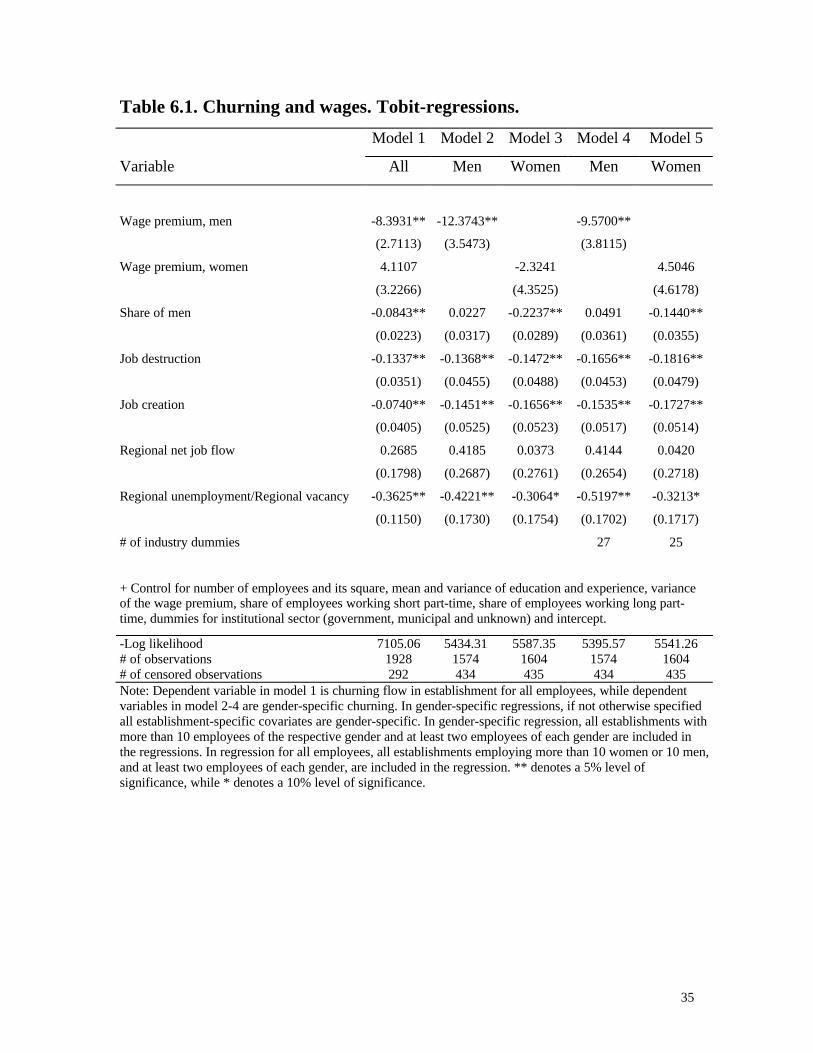
In table 6.1 we report results from several excess turnover or churning

regressions11. Our main focus is on the effect of wages and gender composition on

turnover, and we thus report coefficients for some key variables only12. In the first

column, we report results for the total churning rate of the establishment. We find that the

wage premium of men reduces turnover significantly, while turnover is not significantly

affected by the wage premium of women. This result is strong evidence in favor of the

model of monopsonistic discrimination.

We also find that the share of men reduces turnover significantly, even when the

specification also includes the number of employees and its square. We find that both job

destruction and job creation reduce turnover. If there is job destruction, voluntary quits

and separations add to the decline of the establishment, and lower turnover is observed.

When there is job creation, voluntary quits are likely to be reduced by better prospects

within the firm. We find that turnover is reduced with the local U/V ratio, a result that

supports the job-to-job interpretation of quits.

11 Since churning is zero for a significant proportion of establishments, we use a tobit-specification.12 The regressions also include control for the number of employees, the number of employees squared,the variance of the wage premium, sector, industry (2-digit ISIC), establishment size and its square,establishment specific mean and standard deviation of years of education, and experience, as well as thevariance of the individual wage premiums. Full regression results are available from the authors on request.

35

Table 6.1. Churning and wages. Tobit-regressions.

Model 1 Model 2 Model 3 Model 4 Model 5

Variable All Men Women Men Women

Wage premium, men -8.3931** -12.3743** -9.5700**

(2.7113) (3.5473) (3.8115)

Wage premium, women 4.1107 -2.3241 4.5046

(3.2266) (4.3525) (4.6178)

Share of men -0.0843** 0.0227 -0.2237** 0.0491 -0.1440**

(0.0223) (0.0317) (0.0289) (0.0361) (0.0355)

Job destruction -0.1337** -0.1368** -0.1472** -0.1656** -0.1816**

(0.0351) (0.0455) (0.0488) (0.0453) (0.0479)

Job creation -0.0740** -0.1451** -0.1656** -0.1535** -0.1727**

(0.0405) (0.0525) (0.0523) (0.0517) (0.0514)

Regional net job flow 0.2685 0.4185 0.0373 0.4144 0.0420

(0.1798) (0.2687) (0.2761) (0.2654) (0.2718)

Regional unemployment/Regional vacancy -0.3625** -0.4221** -0.3064* -0.5197** -0.3213*

(0.1150) (0.1730) (0.1754) (0.1702) (0.1717)

# of industry dummies 27 25

+ Control for number of employees and its square, mean and variance of education and experience, varianceof the wage premium, share of employees working short part-time, share of employees working long part-time, dummies for institutional sector (government, municipal and unknown) and intercept.

-Log likelihood 7105.06 5434.31 5587.35 5395.57 5541.26# of observations 1928 1574 1604 1574 1604# of censored observations 292 434 435 434 435Note: Dependent variable in model 1 is churning flow in establishment for all employees, while dependentvariables in model 2-4 are gender-specific churning. In gender-specific regressions, if not otherwise specifiedall establishment-specific covariates are gender-specific. In gender-specific regression, all establishments withmore than 10 employees of the respective gender and at least two employees of each gender are included inthe regressions. In regression for all employees, all establishments employing more than 10 women or 10 men,and at least two employees of each gender, are included in the regression. ** denotes a 5% level ofsignificance, while * denotes a 10% level of significance.

36

The next four columns report results from gender-specific regressions of gender-specific

turnover13. In the first pair of the four columns, we find that men’s turnover is

significantly affected by the firms wage premium for men. Women’s turnover is not

significantly affected by the wage premium for women. The difference between the

coefficients for men and women is significantly different from zero. In the next pair of

columns we have added industry dummies to the regressions. The conclusion with

respect to the difference between men and women is even stronger here: while men’s

turnover is reduced by higher wages within the establishments, women’s turnover is not

significantly affected. The point estimate for women is even positive.

The share of men reduces turnover significantly. It seems, from the separate

regressions, that this effect arises only through reduced turnover for women.

Excess turnover or churning is meant to be a measure of the steady state turnover

of the establishment, rinsed from the direct effect of establishment growth or contraction.

Of course, the world is not in steady state, and the data are rather turbulent with respect to

the growth and decline of establishments. Thus, we have included job flow measures in

the regressions as well.

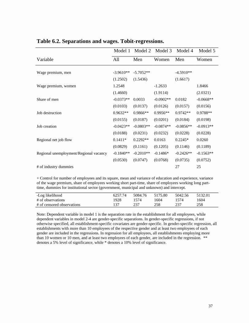
However, to the extent that one may worry about potential effects of using

constructed churning rates rather than actual quit- or separation rates, we also report

results from identical tobit-regressions of the separation rates. Table 6.2 reports results

from these regressions. As job-flow measures are included in the regressions as well, we

do not expect too large differences in the results from the previous table.

We find that the separation rates of the establishment are significantly negatively

affected by the average wage premiums of men, but not so by the average wage premium

calculated for women. Also, the gender-specific separation pattern conforms to our

model. Men’s separations are reduced by higher wages while this is not the case for

women’s separation rates.

We also find that men’s separation rates are sensitive to the job flow of the

regional labor market, while this is not the case for women. This may, of course, be due

13 The sample is limited to establishments with at least 10 employees of the particular gender. In the modelfor all workers, the sample includes establishments where at least one of the groups is represented with 10workers.

37

Table 6.2. Separations and wages. Tobit-regressions.

Model 1 Model 2 Model 3 Model 4 Model 5

Variable All Men Women Men Women

Wage premium, men -3.9610** -5.7052** -4.5910**

(1.2502) (1.5436) (1.6617)

Wage premium, women 1.2548 -1.2633 1.8466

(1.4660) (1.9114) (2.0321)

Share of men -0.0373** 0.0033 -0.0902** 0.0182 -0.0668**

(0.0103) (0.0137) (0.0126) (0.0157) (0.0156)

Job destruction 0.9632** 0.9866** 0.9956** 0.9742** 0.9788**

(0.0155) (0.0187) (0.0201) (0.0184) (0.0198)

Job creation -0.0423** -0.0803** -0.0874** -0.0856** -0.0913**

(0.0188) (0.0231) (0.0232) (0.0228) (0.0228)

Regional net job flow 0.1411* 0.2292** 0.0163 0.2245* 0.0260

(0.0829) (0.1161) (0.1205) (0.1146) (0.1189)

Regional unemployment/Regional vacancy -0.1840** -0.2010** -0.1486* -0.2426** -0.1563**

(0.0530) (0.0747) (0.0768) (0.0735) (0.0752)

# of industry dummies 27 25

+ Control for number of employees and its square, mean and variance of education and experience, varianceof the wage premium, share of employees working short part-time, share of employees working long part-time, dummies for institutional sector (government, municipal and unknown) and intercept.

-Log likelihood 6257.74 5084.76 5175.80 5042.56 5132.01# of observations 1928 1574 1604 1574 1604# of censored observations 137 237 258 237 258

Note: Dependent variable in model 1 is the separation rate in the establishment for all employees, whiledependent variables in model 2-4 are gender-specific separations. In gender-specific regressions, if nototherwise specified, all establishment-specific covariates are gender-specific. In gender-specific regression, allestablishments with more than 10 employees of the respective gender and at least two employees of eachgender are included in the regressions. In regression for all employees, all establishments employing morethan 10 women or 10 men, and at least two employees of each gender, are included in the regression. **denotes a 5% level of significance, while * denotes a 10% level of significance.

38

to compositional differences in the regional job flows, but the result is also consistent

with a notion that a larger portion of female separations are insensitive to labor market

conditions. Furthermore, the effect of the regional U/V-ratio is larger for men than for

women. The results with respect to the share of men in the establishments are similar to

the ones observed in table 6.1.

Now, different types of workers may have different propensity to quit or separate,

and differences in the compositions of workers may affect the separation rates of the

establishment. We have accounted for this, by including the mean and variance of

education and experience of the establishment in the regressions of table 6.1 and 6.2, and

our wage premium is net of the effect of individual characteristics on wages. However, as

a further check on our results, we report in table 6.3 results from regressions of adjusted

separation rates for each establishment. In table 6.3, the dependent variable is the

establishment-specific mean of the residuals from individual regressions of the

probability to separate on education, experience, their squares and interactions, separately

for each gender. The qualitative results are similar to that of the previous table. The

negative effect of wages on male turnover is, however, not significant within industries,

but the difference between men and women is still significant in all specifications.

The results are rather robust with respect to changes in the dependent variable.

Experiments with other wage variables and specifications also give very similar results.

The results are, however, not robust with respect to changes in the sample, in particular,

the results are sensitive to the inclusion of very small establishments, of which there are

many at any given point in time. For smaller establishments it is difficult to find a robust

relationship between wages and turnover (see Barth and Dale-Olsen 1999). In particular,

the results for the relationship between wages and turnover for women turned out very

unstable when we experimented with the sample size. This observation may be due to

statistical properties of small sample-sizes per establishment, but it may also be an

indication of real differences between sub-samples of individuals or establishments in the

economy. However, we leave this issue to future research.

The main weakness of our study is that we have results from one year and one

country only. It remains to be seen if the results are robust enough to show up in longer

series and in other countries as well.

39

Table 6.3. Adjusted separations and wages. OLS-regressions.

Model 1 Model 2 Model 3 Model 4 Model 5

Variable All Men Women Men Women

Wage premium, men -3.3535** -4.3735** -2.6062

(1.31115) (1.5170) (1.6482)

Wage premium, women 1.9946 1.9176 3.7190*

(1.5361) (1.8028) (1.9368)

Share of men -0.0347** -0.0312** -0.0683** -0.0199 -0.0610**

(0.0108) (0.0134) (0.0117) (0.0156) (0.0148)

Job destruction 0.6883** 0.6709** 0.6862** 0.6564** 0.6708**

(0.0163) (0.0188) (0.0193) (0.0187) (0.0193)

Job creation 0.0606** 0.0424* 0.0179 0.0390* 0.0172

(0.0195) (0.0224) (0.0212) (0.0224) (0.0211)

Regional net job flow 0.0543 0.2081* -0.0767 0.1810 -0.0831

(0.0868) (0.1150) (0.1131) (0.1148) (0.1131)

Regional unemployment/Regional vacancy -0.1720** -0.2016** -0.1725** -0.2359** -0.1671**

(0.0554) (0.0736) (0.0723) (0.0732) (0.0717)

# of industry dummies 27 25

+ Control for number of employees and its square, mean and variance of education and experience, varianceof the wage premium, share of employees working short part-time, share of employees working long part-time, dummies for institutional sector (government, municipal and unknown) and intercept.

R2-adj. 0.5176 0.5053 0.4743 0.5226 0.4914

# of observations 1928 1574 1604 1574 1604

Note: Dependent variable in model 1 is the adjusted separation rate in the establishment for all employees,while dependent variables in model 2-4 are gender-specific adjusted separations. In gender-specificregressions, if not otherwise specified, all establishment-specific covariates are gender-specific. In gender-specific regression, all establishments with more than 10 employees of the respective gender and at least twoemployees of each gender are included in the regressions. In regression for all employees, all establishmentsemploying more than 10 women or 10 men, and at least two employees of each gender, are included in theregression. ** denotes a 5% level of significance, while * denotes a 10% level of significance.

40

7. Conclusions

The theory of monopsonistic discrimination was refuted as an explanation of the male-

female wage gap mainly on empirical grounds. Single buyer situations are rare and only

transitory in the labor market, it is not clear that employers are able to differentiate wages

according to gender, and furthermore, female labor supply is at least as wage-elastic as

male labor supply. In this paper, we are able to discard all these caveats, and thus provide

support for the old model of monopsonistic discrimination.

The analysis of labor markets with frictions shows that even in a multi-employer

situation, the supply of labor to any one firm is sensitive to the wage level of that firm.

Given this point, differences in job-to-job search behavior and exogenous separations

from the labor market may produce differences in the elasticity of labor supply facing

each employer. It is then possible for the employer to differentiate between jobs,

occupations or establishments because of differences in the average elasticity of labor

supply between jobs, occupations or establishments.

The empirical part of the paper re-establishes the known fact that occupations or

establishments with a higher proportion of women pay less, even with rather extensive

controls. The novel evidence relates to the results with respect to the wage policy across

establishments. We show that the lower dispersion of residual wages for women arises

from lower wage dispersion across rather than within establishments. This observation is

in line with the predictions from the theoretical model. The employers’ wage policies

towards men and women are positively correlated; high-wage establishments for men are

high-wage establishments for women as well. The wage gap within establishments are

increasing in the share of men and decreasing in the average experience of the

employees.

Our main result is that the turnover and separation rates from the establishments

are more sensitive to the wage premium of men than to that of women. When studying

turnover and separations for men and women separately, we find that the turnover of men

is more sensitive to the establishment-specific wage premium than is the turnover of

women. This difference provides employers with an incentive to employ the policy of

monopsonistic discrimination.

41

Appendix

The data are based on information from several public administrative registers, linked by

Statistics Norway into an integrated register based data system (CSSD). We use a

representative 10 percent sample of all jobs in Norway from 1990. The observations are

grouped by employers, and larger establishments are over-sampled, but the number of

employees per establishment is adjusted to ensure representativeness at the level of jobs.

A detailed description of the data source and sampling plan is given in Barth and Dale-

Olsen (1999a).

Table a1. Descriptive statistics

Mean Standard

deviation

Variables used in wage regressions

N=84,438 individuals

Log(yearly wage) 12.14 0.34

Education 2.80 2.55

Education2 14.30 22.33

Experience 19.99 10.63

Experience2 512.47 460.81

MaleXexperience 13.30 12.82

Seniority 5.52 4.94

Seniority2 54.86 107.74

Male 0.66 0.47

Variables used in turnover regressions

N= 1,928, employers. (1,574 and 1,604

employers in regressions for men and

women respectively, see note)

Regressions for all

employees

Regressions for men Regressions for women

Mean Standard

deviation

Mean Standard

deviation

Mean Standard

deviation

Churning in percent 18.40 16.18 16.70 18.48 18.74 18.39

Quit rate in percent 14.51 13.66 14.61 15.99 15.46 15.15

Adjusted quit rate -4.89 11.23 -3.86 13.25 -5.30 12.66

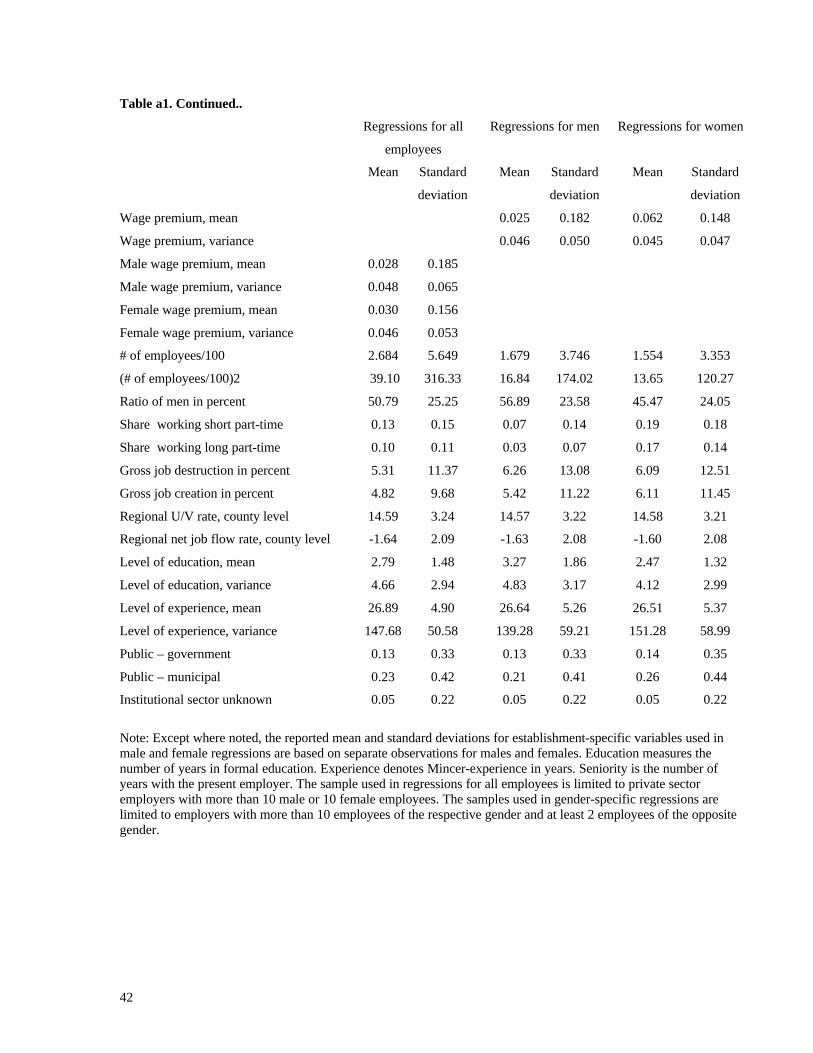
42

Table a1. Continued..

Regressions for all

employees

Regressions for men Regressions for women

Mean Standard

deviation

Mean Standard

deviation

Mean Standard

deviation

Wage premium, mean 0.025 0.182 0.062 0.148

Wage premium, variance 0.046 0.050 0.045 0.047

Male wage premium, mean 0.028 0.185

Male wage premium, variance 0.048 0.065

Female wage premium, mean 0.030 0.156

Female wage premium, variance 0.046 0.053

# of employees/100 2.684 5.649 1.679 3.746 1.554 3.353

(# of employees/100)2 39.10 316.33 16.84 174.02 13.65 120.27

Ratio of men in percent 50.79 25.25 56.89 23.58 45.47 24.05

Share working short part-time 0.13 0.15 0.07 0.14 0.19 0.18

Share working long part-time 0.10 0.11 0.03 0.07 0.17 0.14

Gross job destruction in percent 5.31 11.37 6.26 13.08 6.09 12.51

Gross job creation in percent 4.82 9.68 5.42 11.22 6.11 11.45

Regional U/V rate, county level 14.59 3.24 14.57 3.22 14.58 3.21

Regional net job flow rate, county level -1.64 2.09 -1.63 2.08 -1.60 2.08

Level of education, mean 2.79 1.48 3.27 1.86 2.47 1.32

Level of education, variance 4.66 2.94 4.83 3.17 4.12 2.99

Level of experience, mean 26.89 4.90 26.64 5.26 26.51 5.37

Level of experience, variance 147.68 50.58 139.28 59.21 151.28 58.99

Public – government 0.13 0.33 0.13 0.33 0.14 0.35

Public – municipal 0.23 0.42 0.21 0.41 0.26 0.44

Institutional sector unknown 0.05 0.22 0.05 0.22 0.05 0.22

Note: Except where noted, the reported mean and standard deviations for establishment-specific variables used inmale and female regressions are based on separate observations for males and females. Education measures thenumber of years in formal education. Experience denotes Mincer-experience in years. Seniority is the number ofyears with the present employer. The sample used in regressions for all employees is limited to private sectoremployers with more than 10 male or 10 female employees. The samples used in gender-specific regressions arelimited to employers with more than 10 employees of the respective gender and at least 2 employees of the oppositegender.

43

References

Albæk, Karsten, and Sørensen, Bent S. 1998. “Worker Flows and Job Flows in Danish

Manufacturing, 1980-91” Economic Journal 108:1750-1771.

Barth, Erling, and Dale-Olsen, Harald, 1999a. “The Employer’s Wage Policy and Worker

Turnover.” In Haltiwanger, J.C., J. Lane, J. Spletzer, J. Theeuwes, K.R. Troske,

(eds.), The Creation and Analysis of Matched Employer-Employee Data,

Amsterdam: North Holland, forthcoming.

Barth, Erling, and Dale-Olsen, Harald, 1999b. “ Churning in the Norwegian Labor

Market. Gender Differences in Job and Worker Mobility” In Gustavsson, S. and

D. Meulders (eds.), Gender and the Labor Market. Econometric Evidence on

Obstacles in Achieving Gender Equality. London: Macmillan, forthcoming.

Barth, Erling, and Mastekaasa, Arne, 1996. “Decomposing the Male/Female Wage Gap:

Within and Between Establishments Differences” Labor 10: 339-356.

Barth, Erling, and Schøne, Pål, 1999. “On-the-Job-Training and Worker Turnover – An

Establishment Level Analysis”, Manuscript, Institute for social research, Oslo.

Barth, Erling, and Yin, Hang, 1996. “Promotions, Career Profiles, and the Gender Wage

Gap”, Manuscript, Institute for social research, Oslo.

Blau, Francine, 1977. Equal Pay in the Office. Lexington, MA: DC Heath and Company.

Blau, Francine, Marianne A. Ferber and Anne E. Winkler, 1998. The Economics of

Women, Men and Work. Upper Saddle River, NJ: Prentice Hall.

Blau, Francine, and Kahn, Lawrence, 1981. “Race and sex Differences in Quits by Young

Workers”, Industrial and Labor Relations Review 34: 563-77.

Blau, Francine, and Kahn, Lawrence, 1992. “The Gender Earnings Gap: Learning from

International Comparisons”, American Economic Review 82: 533-538.

Booton, Lavonne and Lane, Julia, 1985. “Hospital Market Structure and the Return to

Nursing Education”, Journal of Human Resources 20: 184-96.

Burdett, Kenneth, and Mortensen, Dale, 1998. “Equilibrium Wage Differentials and

Employer Size.” International Economic Review 39:257-73.

44

Burgess, Simon; Lane, Julia; and Stevens, David, 1996. “Job Flows and Worker Flows:

Issues and Evidence from a Panel of Firms.” In The flow analysis of labor

markets. Studies in the Modern World Economy, vol. 3 edited by Ronald

Schettcat. London and New York: Routledge,

Davis, Steven J.; Haltiwanger, John; and Schuh, Scott, 1996. Job Creation and

Destruction. Cambridge and London: MIT Press.

Ferber, Marianne; Loeb, Jane; and Lowry, Helen, 1978. “The Economic Status of

Women Faculty: A Reappraisal.” Journal of Human Resources 13: 385-401.

Galizzi, Monica, 1998. “Gender Differences in Quit Behavior: Do Future Wages Matter?

An analysis for short-tenure workers.” Manuscript, Workers Compensation

Research Institute, Cambridge MA.

Goldin, Claudia, 1986. “Monitoring Costs and Occupational Segregation by Sex: A

Historical Analysis”. Journal of Labor Economics 4:1-26.

Groshen, Erica L. 1991. “Sources of Intra-Industry Wage Dispersion: How Much Do

Employers Matter?” Quarterly Journal of Economics 106:869-84.

Hamermesh, Daniel S., and Goldfarb, Robert S. 1970. “Manpower programs in a Local

Labor Market: A Theoretical Note.” American Economic Review 60:706-709.

Humphries, Jane, 1995. “Economics, Gender and Equal Opportunities”. In The

Economics of Equal Opportunities edited by Jane Humphries and Jill Rubury.

Manchester: Equal Opportunities Commission.

Keith, Kristen, and Abagail McWilliams, 1999. “The returns to mobility and job search

by gender”, Industrial and Labor Relations Review, Vol. 52(3):463-474.

Lane, Julia; Isaac, Alan; and Stevens, David, 1996. “Firm Heterogeneity and Worker

Turnover”, Review of Industrial Organization vol. 11:275-291.

Lazear, Edward, and Rosen, Sherwin, 1990. “Male-Female Wage Differentials in Job

Ladders”, Journal of Labor Economics 8: S106-23.

Leonard, Jonathan, and Audenrode, Marc, 1996. “Worker’s Limited Liability, Turnover

and Employment Contracts”, Annales d’Economie et de Statistique, 41/42:41-78.

Loprest, Pamela J. 1993, “Gender Differences in Wage Growth and Job Mobility”,

American Economic Review, vol. 821:526-532.

45

Lucifora, Claudio and Reilly, Barry. 1990. “Wage Discrimination and Female

Occupational Intensity”, Labor 4: 147-68.

Lynch, Lisa M. 1991, “The Role of Off-the-Job vs. On-the-Job Training for the Mobility

of Women Workers”, American Economic Review, vol. 80:151-156.

Manning, Alan, 1994. “Labor Markets with Company Wage Policies”, Discussion Paper

no. 214. London: Centre for Economic Performance.

Madden, Janice F. 1973, The Economics of Sex Discrimination, Lexington MA:

Lexington Books.

Polachek, Salomon W. 1981. “Occupational Self-Selection: A Human Capital Approach

to Sex Differences in Occupational Structure”, Review of Economics and

Statistics 63: 60-69.

Petersen, Trond and Morgan, Laurie A. 1995. “Separate and unequal: Occupation-

Establishment Sex Segregation and the Gender Wage Gap”, American Journal of

Sociology 101: 329-365.

Pissarides, Christopher A. and Jonathan Wadsworth, 1994. “On-the-job search, Some

empirical evidence from Britain”, European Economic Review, Vol. 38:385-401.

Robinson, Joan. 1933. The Economics of Imperfect Competition. London: Macmillan.

Salop, Steven C. 1979. “A Model of the Natural Rate of Unemployment”, American

Economic Review 69:117-125.

Schøne, Pål, 1999. “Training and on-the-job search, An empirical analysis”, Manuscript,

Institute for social research, Oslo.

Sicherman, Nachum, 1996. “Gender Differences in Departures from a Large Firm”,

Industrial and Labor Relations Review, Vol. 49:484-505.

Viscusi, W. Kip, 1979. “Sex Differences in Worker Quitting”, The Review of Economics

and Statistics, vol. 62:388-398.

</ref_section>