1 Introduction

Multidisciplinary design optimization (MDO): a field of engineering thatuses numerical optimization to perform the design of systems that involve anumber of disciplines or subsystems.

• the best design of a multidisciplinary system can only be found when theinteractions between the system’s disciplines are fully considered.

• Considering these interactions in the design process cannot be done in anarbitrary way

• requires a sound mathematical formulation.

By solving the MDO problem early in the design process and taking advantageof advanced computational analysis tools, designers can simultaneously improvethe design and reduce the time and cost of the design cycle.

1

The origins of MDO can be traced back to Schmit [131, 132, 133] andHaftka [55, 56, 58], who extended their experience in structural optimization toinclude other disciplines.

One of the first applications of MDO was aircraft wing design, whereaerodynamics, structures, and controls are three strongly coupleddisciplines [51, 52, 100, 99].

Since then, the application of MDO has been extended:

• complete aircraft [88, 102], rotorcraft [45, 49], and spacecraft [23, 27].

• bridges [9] and buildings [32, 47];

• railway cars [64, 42], automobiles [109, 85], and ships [123, 70];

• and even microscopes [124].

2

Important considerations when implementing MDO:

• How to organize the disciplinary analysis models?

• What optimization software/methods do we choose?

• Do we use approximation (surrogate) models?

MDO architecture: Combination of problem formulation and organizationalstrategy. The MDO architecture defines both how the different models arecoupled and how the overall optimization problem is solved.

There are several terms in literature used to describe what we mean by“architecture” [22, 87, 138, 30]:

• “method”[88, 144, 158, 128, 1],

• “methodology”[77, 114, 112],

• “problem formulation”[35, 4, 5],

• “strategy”[161, 59],

• “procedure”[145, 81] and

• “algorithm”[135, 143, 137, 41]

3

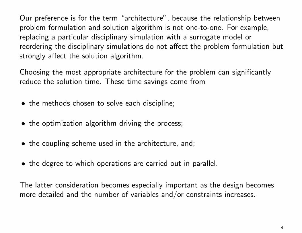
Our preference is for the term “architecture”, because the relationship betweenproblem formulation and solution algorithm is not one-to-one. For example,replacing a particular disciplinary simulation with a surrogate model orreordering the disciplinary simulations do not affect the problem formulation butstrongly affect the solution algorithm.

Choosing the most appropriate architecture for the problem can significantlyreduce the solution time. These time savings come from

• the methods chosen to solve each discipline;

• the optimization algorithm driving the process;

• the coupling scheme used in the architecture, and;

• the degree to which operations are carried out in parallel.

The latter consideration becomes especially important as the design becomesmore detailed and the number of variables and/or constraints increases.

4

The purpose of this chapter:

• survey the available MDO architectures

• present architectures in a unified notation to facilitate understanding andcomparison

• introduce the Extended Design Structure Matrix (XDSM), a diagram tovisualize the algorithm of a given MDO architecture

5

2 Unified Description of MDO Architectures

2.1 Terminology and Mathematical Notation

design variable: a variable in the MDO problem that is always under theexplicit control of an optimizer.

local design variable: design variables relevant to a single discipline only→ denoted by xi for discipline i

shared design variable: design variables used by several disciplines→ denoted by x0

Full set of design variables:

x =[xT0 , x

T1 , . . . , x

TN

]TThink of some examples of local and shared design variables in the context ofaerostructural optimization

6

discipline analysis: a simulation that models the behavior of one aspect of amultidisciplinary system→ represented by equations Ri = 0,

state variables: set of variables determined by solving a discipline analysis.→ denoted by yi

Give some examples of aerodynamic discipline analyses. What are thecorresponding state variables?

7

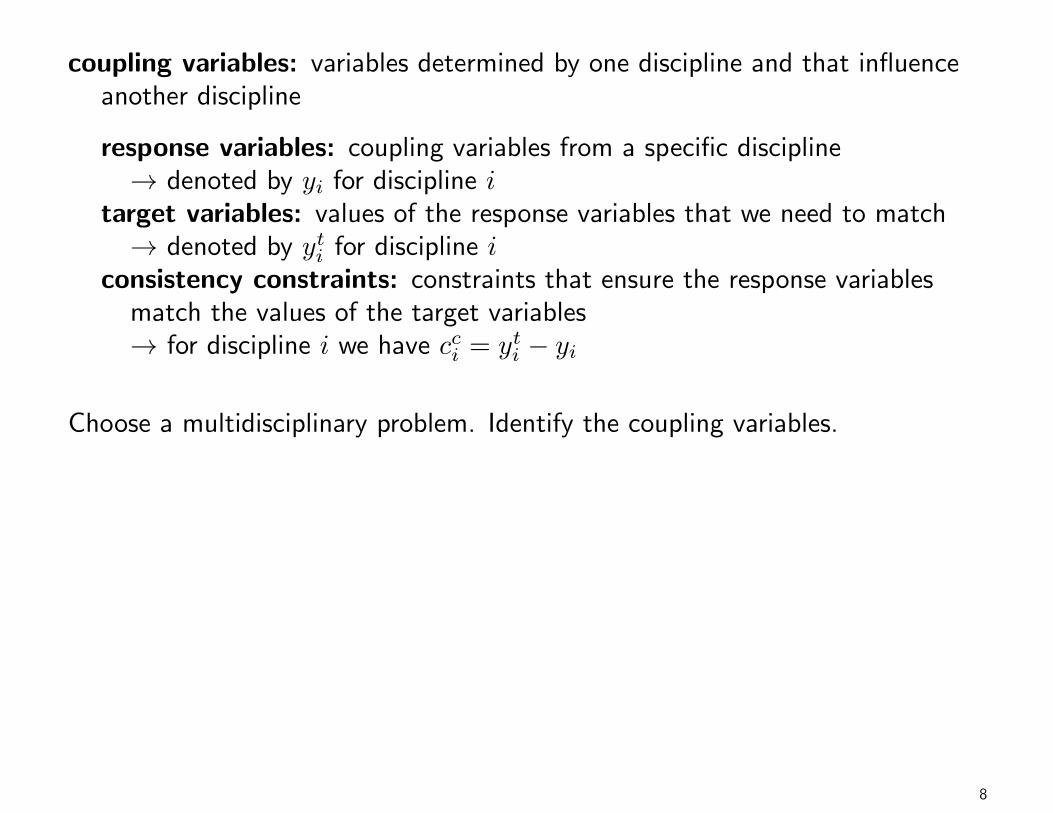
coupling variables: variables determined by one discipline and that influenceanother discipline

response variables: coupling variables from a specific discipline→ denoted by yi for discipline i

target variables: values of the response variables that we need to match→ denoted by yti for discipline i

consistency constraints: constraints that ensure the response variablesmatch the values of the target variables→ for discipline i we have cci = yti − yi

Choose a multidisciplinary problem. Identify the coupling variables.

8

Table 1: Mathematical notation for MDO problem formulations

Symbol Definitionx Vector of design variablesyt Vector of coupling variable targets (inputs to a discipline analysis)y Vector of coupling variable responses (outputs from a discipline analysis)y Vector of state variables (variables used inside only one discipline analysis)f Objective functionc Vector of design constraintscc Vector of consistency constraintsR Governing equations of a discipline analysis in residual formN Number of disciplinesn() Length of given variable vectorm() Length of given constraint vector()0 Functions or variables that are shared by more than one discipline()i Functions or variables that apply only to discipline i()∗ Functions or variables at their optimal value

() Approximation of a given function or vector of functions

9

2.2 Architecture Diagrams — The Extended DesignStructure Matrix

An Extended Design Structure Matrix, or XDSM [89], is a convenient andcompact way to describe the sequence of operations in an MDO architecture.The XDSM was developed to simultaneously communicate data dependencyand process flow between computational components of the architecture on asingle diagram

The XDSM is based on Design Structure Matrix [146, 25] and follows its basicrules:

• architecture components are placed on main diagonal of the “matrix”

• inputs to a component are placed in the same column

• outputs to a component are placed in the same row

• External inputs and outputs may also be defined and are placed on the outeredges of the diagram

10

• Thick gray lines are used to show the data flow between components

• A numbering system is used to show the order in which the components areexecuted (The algorithm starts at component zero and proceeds in numericalorder)

• consecutive components in the algorithm are connected by a thin black line

• Loops are denoted using the notation j → k for k < j so that the algorithmmust return to step k until a looping condition is satisfied before proceeding

11

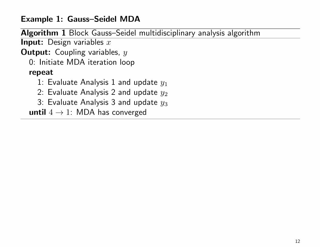
Example 1: Gauss–Seidel MDA

Algorithm 1 Block Gauss–Seidel multidisciplinary analysis algorithmInput: Design variables xOutput: Coupling variables, y

0: Initiate MDA iteration looprepeat

1: Evaluate Analysis 1 and update y12: Evaluate Analysis 2 and update y23: Evaluate Analysis 3 and update y3

until 4→ 1: MDA has converged

12

yt x0, x1 x0, x2 x0, x3

(no data)0,4→1:MDA

1 : yt2, yt3 2 : yt3

y1 4 : y11:

Analysis 12 : y1 3 : y1

y2 4 : y22:

Analysis 23 : y2

y3 4 : y33:

Analysis 3

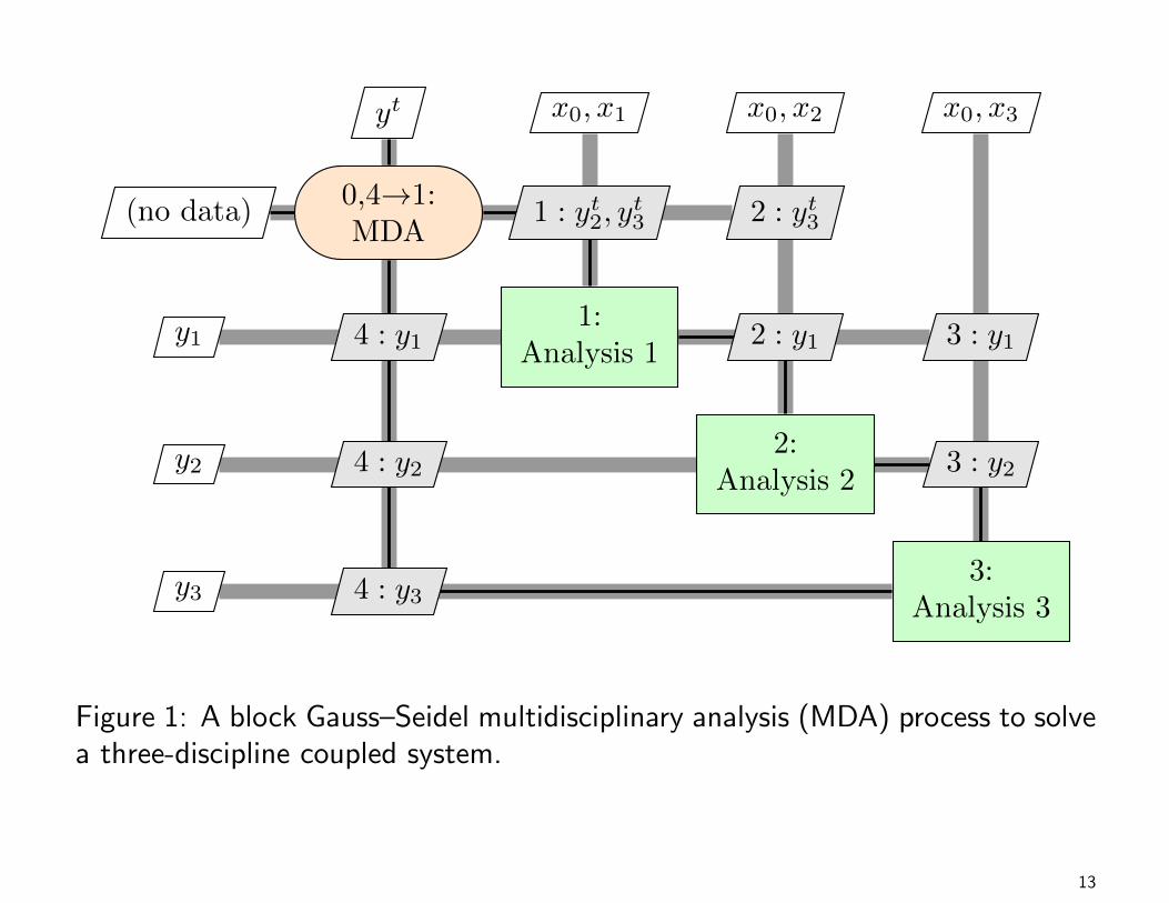
Figure 1: A block Gauss–Seidel multidisciplinary analysis (MDA) process to solvea three-discipline coupled system.

13

Example 2: Gradient-based Optimization

• objective, constraints, and gradient evaluations are the (3) individualcomponents

14

Example 2: Gradient-based Optimization

• objective, constraints, and gradient evaluations are the (3) individualcomponents

x(0)

x∗ 0,2→1:Optimization

1 : x 1 : x 1 : x

2 : f1:

Objective

2 : c1:

Constraints

2 : df/dx, dc/dx1:

Gradients

Figure 2: A gradient-based optimization procedure.

15

2.3 The All-At-Once (AAO) Problem Statement

Consider the general “all-at-once” (AAO) MDO problem statement:

minimize f0 (x, y) +

N∑i=1

fi (x0, xi, yi)

with respect to x, yt, y, y

subject to c0 (x, y) ≥ 0

ci (x0, xi, yi) ≥ 0 for i = 1, . . . , N

cci = yti − yi = 0 for i = 1, . . . , N

Ri

(x0, xi, y

tj 6=i, yi, yi

)= 0 for i = 1, . . . , N.

• Typically omit the local objective functions fi unless necessary

• Some authors refer to AAO as simultaneous analysis and design

• AAO is rarely solved in practice: we can eliminate the cci .

16

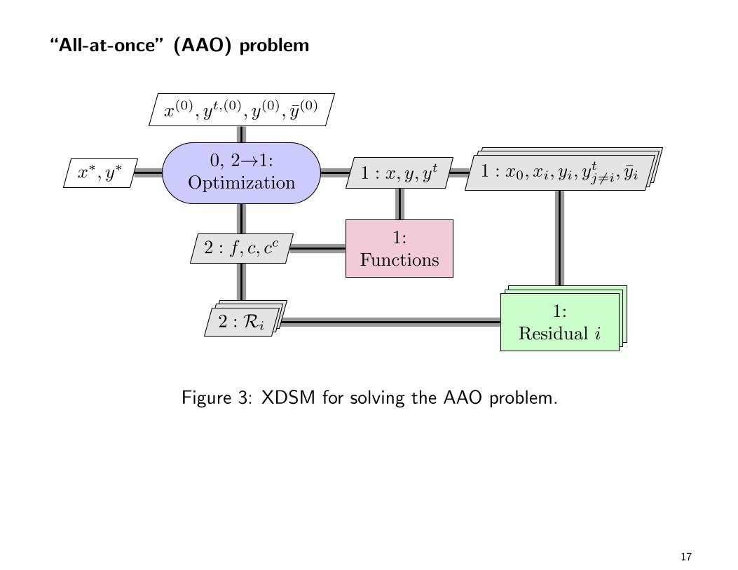
“All-at-once” (AAO) problem

x(0), yt,(0), y(0), y(0)

x∗, y∗0, 2→1:

Optimization1 : x, y, yt 1 : x0, xi, yi, y

tj 6=i, yi

2 : f, c, cc1:

Functions

2 : Ri1:

Residual i

Figure 3: XDSM for solving the AAO problem.

17

3 Monolithic Architectures

AAO provides a unifying starting point for other architectures; depending onwhich constraints are eliminated, we can derive different monolithicarchitectures.

Monolithic Architectures: an architecture that the solves the MDO problemas a single optimization problem.

We will consider three monolithic architectures:

1. Simultaneous Analysis and Design (SAND);

2. Individual Discipline Feasible (IDF), and;

3. Multidisciplinary Feasible (MDF).

The monolithic architectures are distinguished by how they achievemultidisciplilnary feasibility.

18

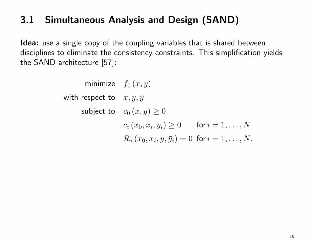
3.1 Simultaneous Analysis and Design (SAND)

Idea: use a single copy of the coupling variables that is shared betweendisciplines to eliminate the consistency constraints. This simplification yieldsthe SAND architecture [57]:

minimize f0 (x, y)

with respect to x, y, y

subject to c0 (x, y) ≥ 0

ci (x0, xi, yi) ≥ 0 for i = 1, . . . , N

Ri (x0, xi, y, yi) = 0 for i = 1, . . . , N.

19

Simultaneous Analysis and Design

x(0), y(0), y(0)

x∗, y∗0,2→1:

Optimization1 : x, y 1 : x0, xi, y, yi

2 : f, c1:

Functions

2 : Ri1:

Residual i

Figure 4: Diagram for the SAND architecture.

20

Several features of the SAND architecture are noteworthy:

• The optimizer is responsible for simultaneously analyzing and designing thesystem

• At each iteration, the analyses do not need to be solved exactly: Ri 6= 0→ inexact solution to analyses: potential to solve optimization quickly→ 5-10 times a single MDA

• Can also be used to solve single discipline optimization problem

• Full-space PDE-constrained optimization is an example

Question: Can you think of some disadvantages of SAND?

21

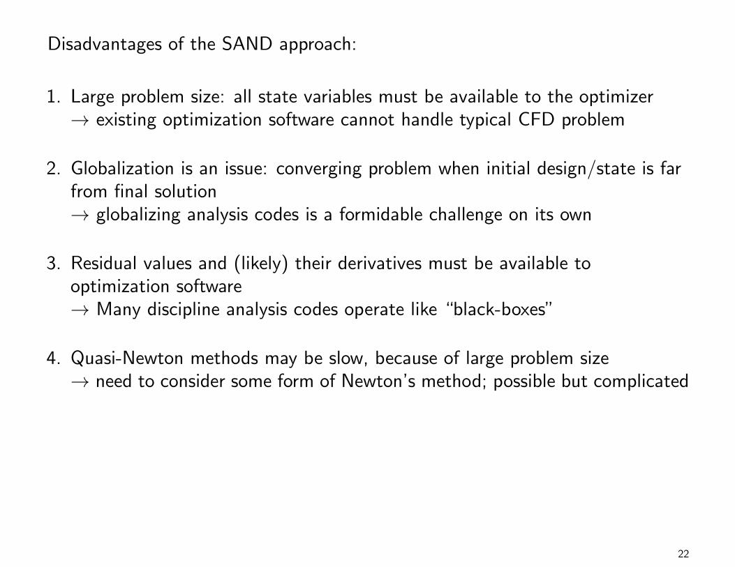
Disadvantages of the SAND approach:

1. Large problem size: all state variables must be available to the optimizer→ existing optimization software cannot handle typical CFD problem

2. Globalization is an issue: converging problem when initial design/state is farfrom final solution→ globalizing analysis codes is a formidable challenge on its own

3. Residual values and (likely) their derivatives must be available tooptimization software→ Many discipline analysis codes operate like “black-boxes”

4. Quasi-Newton methods may be slow, because of large problem size→ need to consider some form of Newton’s method; possible but complicated

22

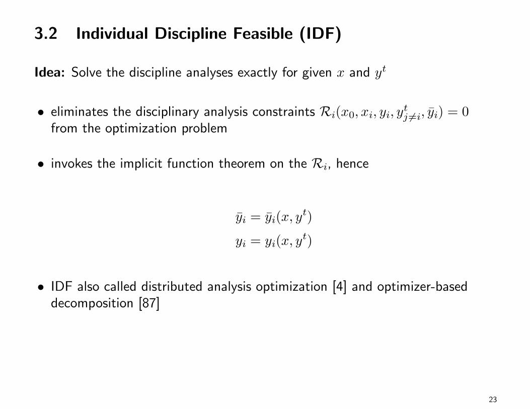
3.2 Individual Discipline Feasible (IDF)

Idea: Solve the discipline analyses exactly for given x and yt

• eliminates the disciplinary analysis constraints Ri(x0, xi, yi, ytj 6=i, yi) = 0

from the optimization problem

• invokes the implicit function theorem on the Ri, hence

yi = yi(x, yt)

yi = yi(x, yt)

• IDF also called distributed analysis optimization [4] and optimizer-baseddecomposition [87]

23

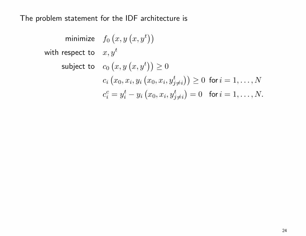
The problem statement for the IDF architecture is

minimize f0(x, y

(x, yt

))with respect to x, yt

subject to c0(x, y

(x, yt

))≥ 0

ci(x0, xi, yi

(x0, xi, y

tj 6=i

))≥ 0 for i = 1, . . . , N

cci = yti − yi(x0, xi, y

tj 6=i

)= 0 for i = 1, . . . , N.

24

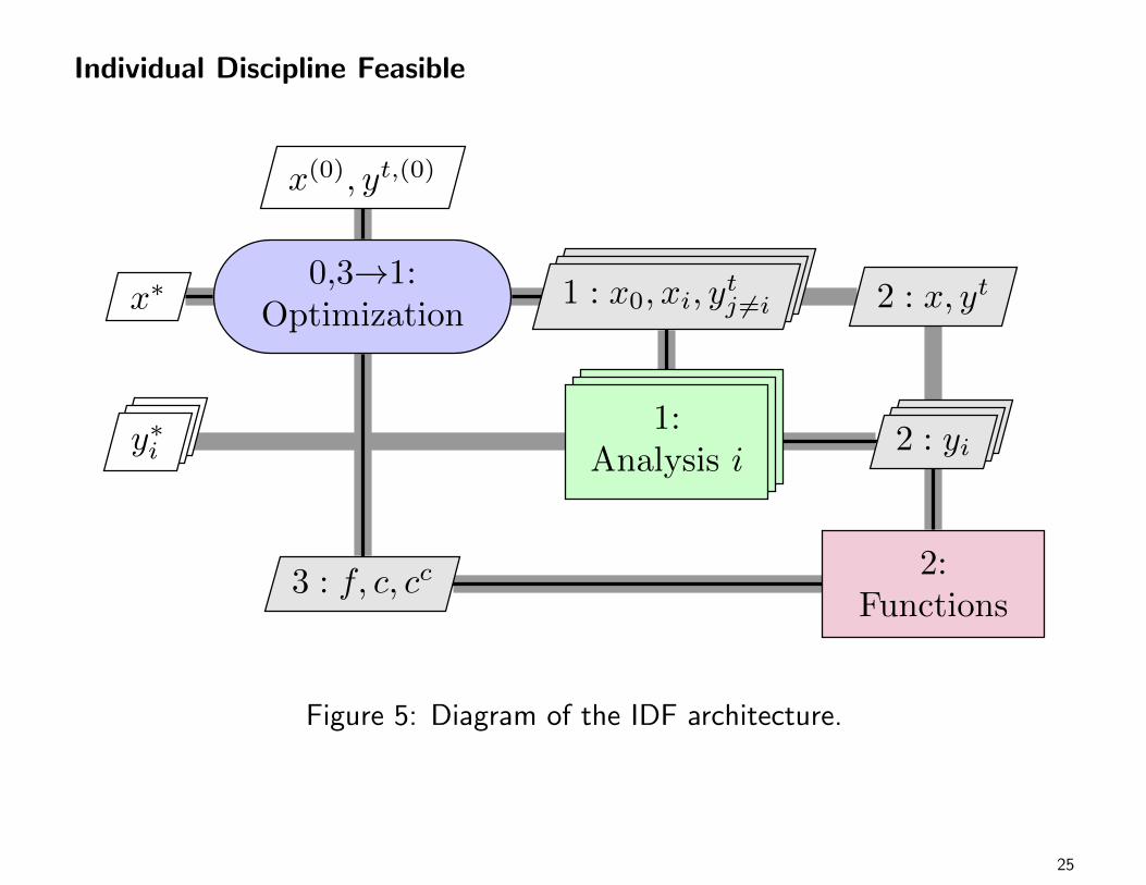
Individual Discipline Feasible

x(0), yt,(0)

x∗0,3→1:

Optimization1 : x0, xi, y

tj 6=i 2 : x, yt

y∗i1:

Analysis i2 : yi

3 : f, c, cc2:

Functions

Figure 5: Diagram of the IDF architecture.

25

Some advantages of IDF include the following:

• all state variables and discipline analysis equations are removed fromoptimization

• discipline analyses can be performed in parallel

• analysis codes are already highly specialized and efficient at solving theirrespective equations→ for example, globalization is simplified

The increased flexibility of IDF comes at a price. List some of the drawbacks ofthis architecture?

26

Disadvantages of IDF:

1. if optimization terminates before satisfying the KKT conditions (forexample), the intermediate solution is not multidisciplinary feasible→ in some sense, this is no better than SAND

2. number of coupling variables may still be large→ typically 103 – 105 for aerostructural problems

3. gradient computation, if necessary, is expensive→ Adjoint-based gradients are critical for efficiency, but requires intrusioninto source code

27

3.3 Multidisciplinary Feasible (MDF)

Idea: Solve the multidisciplinary analysis exactly for given x.

• eliminate both the disciplinary analyses and consistency constraints fromoptimization problem

• also called Fully Integrated Optimization [4] and Nested Analysis andDesign [10]

MDF problem statement:

minimize f0 (x, y (x, y))

with respect to x

subject to c0 (x, y (x, y)) ≥ 0

ci (x0, xi, yi (x0, xi, yj 6=i)) ≥ 0 for i = 1, . . . , N.

28

Multidisciplinary Feasible

x(0) yt,(0)

x∗ 0, 7→1:Optimization

2 : x0, x1 3 : x0, x2 4 : x0, x3 6 : x

1, 5→2:MDA

2 : yt2, yt3 3 : yt3

y∗1 5 : y12:

Analysis 13 : y1 4 : y1 6 : y1

y∗2 5 : y23:

Analysis 24 : y2 6 : y2

y∗3 5 : y34:

Analysis 36 : y3

7 : f, c6:

Functions

Figure 6: Diagram for the MDF architecture with a Gauss–Seidel multidisciplinaryanalysis.

29

Advantageous features of MDF:

• optimization algorithm is responsible for the design variables, objective, anddesign constraints only→ optimization problem is as small as possible

• design is always feasible in a multidisciplinary sense

The MDA can be solved in various ways, but efficiency of optimization is tied tothis choice:

• simple, popular choice is a fixed-point iteration like Gauss-Seidel

• Newton-Krylov approach is much more efficient, but requires intrusion

What about disadvantages of MDF?

30

Drawbacks of using MDF:

1. architecture requires full MDA for each (optimization) iterationMDA is, on its own, a challenging task→ may not be an issue if only one discipline dominates CPU time

2. gradient computation is complex→ for efficiency, need a coupled adjoint for whole MDA

3. For premature iteration state variables are feasible, but design may not be→ dependent on choice of optimization algorithm

31

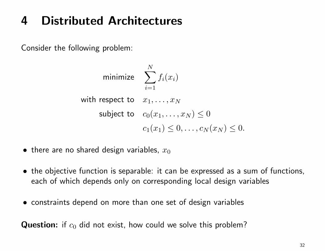
4 Distributed Architectures

Consider the following problem:

minimizeN∑i=1

fi(xi)

with respect to x1, . . . , xN

subject to c0(x1, . . . , xN) ≤ 0

c1(x1) ≤ 0, . . . , cN(xN) ≤ 0.

• there are no shared design variables, x0

• the objective function is separable: it can be expressed as a sum of functions,each of which depends only on corresponding local design variables

• constraints depend on more than one set of design variables

Question: if c0 did not exist, how could we solve this problem?

32

The previous problem is referred to as a complicating constraints problem [33].

Another possibility:

minimizeN∑i=1

fi(x0, xi)

with respect to x0, x1, . . . , xN

subject to c1(x0, x1) ≤ 0, . . . , cN(x0, xN) ≤ 0.

This is referred to as a problem with complicating variables [33].

• Decomposition would be straightforward if there were no shared designvariables, x0, and we could solve N optimization problems independently andin parallel.

33

Distributed Architectures: an architecture that the solves the MDO problemusing a set of optimization problems or subproblems.

The primary motivation for decomposing the MDO problem comes from thestructure of the engineering design environment.

• typical industrial practice involves breaking up the design of a large systemand distributing aspects of that design to specific engineering groups.

• These groups may be geographically distributed and may only communicateinfrequently.

• These groups typically like to retain control of their own design proceduresand make use of in-house expertise; they object to a central designauthority [87].

Decomposition through distributed architectures allow individual design groupsto work in isolation, controlling their own sets of design variables, whileperiodically updating information from other groups to improve their aspect ofthe overall design. This approach to solving the problem conforms more closelywith current industrial design practice than the approach of the monolithicarchitectures.

34

4.1 Classification

Previous classifications of MDO architectures:

• based on observations of which constraints were available to the optimizer tocontrol [10, 3].

• Alexandrov and Lewis [3] used the term “closed” to denote when a set ofconstraints cannot be satisfied by explicit action of the optimizer, and“open” otherwise.For example, the MDF architecture is closed with respect to both analysisand consistency constraints, because their satisfaction is determined throughthe process of converging the MDA. Similarly, IDF is closed analysis butopen consistency since the consistency constraints can be satisfied by theoptimizer adjusting the coupling targets and design variables.

• Tosserams et al. [154] expanded on this classification scheme by discussingwhether or not distributed architectures used open or closed local designconstraints in the system subproblem.

35

Closure of the constraints is an important consideration when selecting anarchitecture because most robust optimization software will permit theexploration of infeasible regions of the design space. Such exploration mayresult in faster solutions via fewer optimizer iterations, but this must be weighedagainst the increased optimization problem size and the risk of terminating theoptimization at an infeasible point.

36

New classification for distributed MDO architectures: a distributed MDOarchitecture can be classified based on their monolithic analogues: either MDF,IDF, or SAND.

This stems from the different approaches to handling the state and couplingvariables in the monolithic architectures.

• similar to the previous classifications in that an equality constraint must beremoved from the optimization problem — i.e., closed — for every variableremoved from the problem statement.

• However, using a classification based on the monolithic architectures makesit much easier to see the connections between distributed architectures, evenwhen these architectures are developed in isolation from each other.

In many cases, the problem formulations in the distributed architecture can bederived directly from that of the monolithic architecture by adding certainelements to the problem, by making certain assumptions, and by applying aspecific decomposition scheme. This classification can also be viewed as aframework in which we can develop new distributed architectures, since thestarting point for a distributed architecture is always a monolithic architecture.

37

AAO SAND

IDF MDF

Monolithic

CSSO

BLISS

MDOIS

ASO

Distributed MDF

QSD

CO

BLISS-2000ATC

IPD/EPD

ECO

Distributed IDF

Penalty Multilevel

Figure 7: Classification of the MDO architectures.

38

Some notes on the classification diagram:

• Known relationships between the architectures are shown by arrows.

• we have only included the “core”architectures in our diagram. Details on theavailable variations for each distributed architecture are presented in therelevant sections.

• Note that none of the distributed architectures developed to date have beenconsidered analogues of SAND.

• Our classification scheme does not distinguish between the different solutiontechniques for the distributed optimization problems. For example, we havenot focused on the order in which the distributed problems are solved.Coordination schemes are partially addressed in the Distributed IDF group,where we have classified the architectures as either “penalty” or “multilevel”,based on whether penalty functions or a problem hierarchy is used in thecoordination. This grouping follows from the work of de Wit and vanKeulen [38].

39

The following sections introduce the distributed architectures for MDO.

• We prefer to use the term “distributed” as opposed to “hierarchical” or“multilevel” because these architectures do not necessarily create a hierarchyof problems to solve.

• Furthermore, neither the systems being designed nor the design teamorganization need to be hierarchical in nature for these architectures to beapplicable.

• Our focus here is to provide a unified description of these architectures andexplain some advantages and disadvantages of each. Along the way, we willpoint out variations and applications of each architecture that can be foundin the literature.

• We also aim to review the state-of-the-art in architectures, since the mostrecent detailed architecture survey in the literature dates back from morethan a decade ago [145]. More recent surveys, such as that of Agte et al. [1],discuss MDO more generally without detailing the architectures themselves.

40

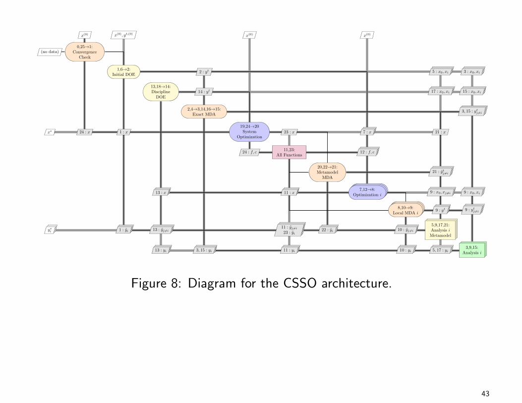
4.2 Concurrent Subspace Optimization (CSSO)

• CSSO is one of the oldest distributed architectures for large-scale MDOproblems.

• The original formulation [139, 18] decomposes the system problem intoindependent subproblems with disjoint sets of variables.

• Global sensitivity information is calculated at each iteration to give eachsubproblem a linear approximation to a multidisciplinary analysis, improvingthe convergence behavior.

• At the system level, a coordination problem is solved to recompute the“responsibility”, “tradeoff”, and “switch” coefficients assigned to eachdiscipline to provide information on design variable preferences for nonlocalconstraint satisfaction. Using these coefficients gives each discipline a certaindegree of autonomy within the system as a whole.

41

The version we consider here, due to Sellar et al. [135], uses metamodelrepresentations of each disciplinary analysis to efficiently model multidisciplinaryinteractions. Using our unified notation, the CSSO system subproblem is givenby

minimize f0 (x, y (x, y))

with respect to x

subject to c0 (x, y (x, y)) ≥ 0

ci (x0, xi, yi (x0, xi, yj 6=i)) ≥ 0 for i = 1, . . . , N

(1)

and the discipline i subproblem is given by

minimize f0 (x, yi (xi, yj 6=i) , yj 6=i)

with respect to x0, xi

subject to c0 (x, y (x, y)) ≥ 0

ci (x0, xi, yi (x0, xi, yj 6=i)) ≥ 0

cj (x0, yj (x0, y)) ≥ 0 for j = 1, . . . , N j 6= i.

(2)

42

x(0) x(0), yt,(0) x(0) x(0)

(no data)0,25→1:

ConvergenceCheck

1,6→2:Initial DOE

2 : yt 5 : x0, xi 3 : x0, xi

13,18→14:Discipline

DOE14 : yt 17 : x0, xi 15 : x0, xi

2,4→3,14,16→15:Exact MDA

3, 15 : ytj 6=i

x∗ 24 : x 1 : x

19,24→20System

Optimization23 : x 7 : x 21 : x

24 : f, c11,23:

All Functions12 : f, c

20,22→21:Metamodel

MDA

21 : ytj 6=i

13 : x 11 : x7,12→8:

Optimization i9 : x0, xj 6=i 9 : x0, xi

8,10→9:Local MDA i

9 : yt 9 : ytj 6=i

y∗i 1 : yi 13 : yj 6=i11 : yj 6=i

23 : yi22 : yi 10 : yj 6=i

5,9,17,21:Analysis iMetamodel

13 : yi 3, 15 : yi 11 : yi 10 : yi 5, 17 : yi3,9,15:

Analysis i

Figure 8: Diagram for the CSSO architecture.

43

Algorithm 2 CSSOInput: Initial design variables xOutput: Optimal variables x∗, objective function f∗, and constraint values c∗

0: Initiate main CSSO iterationrepeat

1: Initiate a design of experiments (DOE) to generate design pointsfor Each DOE point do

2: Initiate an MDA that uses exact disciplinary informationrepeat

3: Evaluate discipline analyses4: Update coupling variables y

until 4→ 3: MDA has converged5: Update the disciplinary metamodels with the latest design

end for 6→ 27: Initiate independent disciplinary optimizations (in parallel)for Each discipline i do

repeat8: Initiate an MDA with exact coupling variables for discipline i and approximate coupling variables for the other disciplinesrepeat

9: Evaluate discipline i outputs yi, and metamodels for the other disciplines, yj 6=iuntil 10→ 9: MDA has converged11: Compute objective f0 and constraint functions c using current data

until 12→ 8: Disciplinary optimization i has convergedend for13: Initiate a DOE that uses the subproblem solutions as sample pointsfor Each subproblem solution i do

14: Initiate an MDA that uses exact disciplinary informationrepeat

15: Evaluate discipline analyses.until 16→ 15 MDA has converged17: Update the disciplinary metamodels with the newest design

end for 18→ 1419: Initiate system-level optimizationrepeat

20: Initiate an MDA that uses only metamodel informationrepeat

21: Evaluate disciplinary metamodelsuntil 22→ 21: MDA has converged23: Compute objective f , and constraint function values c

until 24→ 20: System level problem has convergeduntil 25→ 1: CSSO has converged

44

A potential pitfall of CSSO architecture is the necessity of including all designvariables in the system subproblem. For industrial-scale design problems, thismay not always be possible or practical.

There have been some benchmarks comparing CSSO with other MDOarchitectures. Perez et al., [121] Yi et al. [162], and Tedford and Martins [150]all show CSSO requiring many more analysis calls than other architectures toconverge to an optimal design. The results of de Wit and van Keulen [37]showed that CSSO was unable to reach the optimal solution of even a simpleminimum-weight two-bar truss problem. Thus, CSSO seems to be largelyineffective when compared with newer MDO architectures.

45

4.3 Collaborative Optimization (CO)

• In CO, the disciplinary optimization problems are formulated to beindependent of each other by using target values of the coupling and shareddesign variables [20, 21].

• These target values are then shared with all disciplines during every iterationof the solution procedure.

• The complete independence of disciplinary subproblems combined with thesimplicity of the data-sharing protocol makes this architecture attractive forproblems with a small amount of shared data.

46

x(0)0 , x

(0)1···N , yt,(0) x

(0)0i , x

(0)i

x∗0

0, 2→1:System

Optimization1 : x0, x1···N , yt 1.1 : ytj 6=i 1.2 : x0, xi, y

t

2 : f0, c0

1:System

Functions

x∗i1.0, 1.3→1.1:Optimization i

1.1 : x0i, xi 1.2 : x0i, xi

y∗i1.1:

Analysis i1.2 : yi

2 : J∗i 1.3 : fi, ci, Ji

1.2:Discipline iFunctions

Figure 9: Diagram for the CO architecture.

47

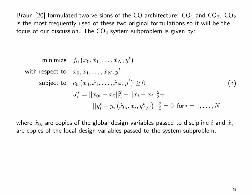
Braun [20] formulated two versions of the CO architecture: CO1 and CO2. CO2

is the most frequently used of these two original formulations so it will be thefocus of our discussion. The CO2 system subproblem is given by:

minimize f0(x0, x1, . . . , xN , y

t)

with respect to x0, x1, . . . , xN , yt

subject to c0(x0, x1, . . . , xN , y

t)≥ 0

J∗i = ||x0i − x0||22 + ||xi − xi||22+||yti − yi

(x0i, xi, y

tj 6=i

)||22 = 0 for i = 1, . . . , N

(3)

where x0i are copies of the global design variables passed to discipline i and xiare copies of the local design variables passed to the system subproblem.

48

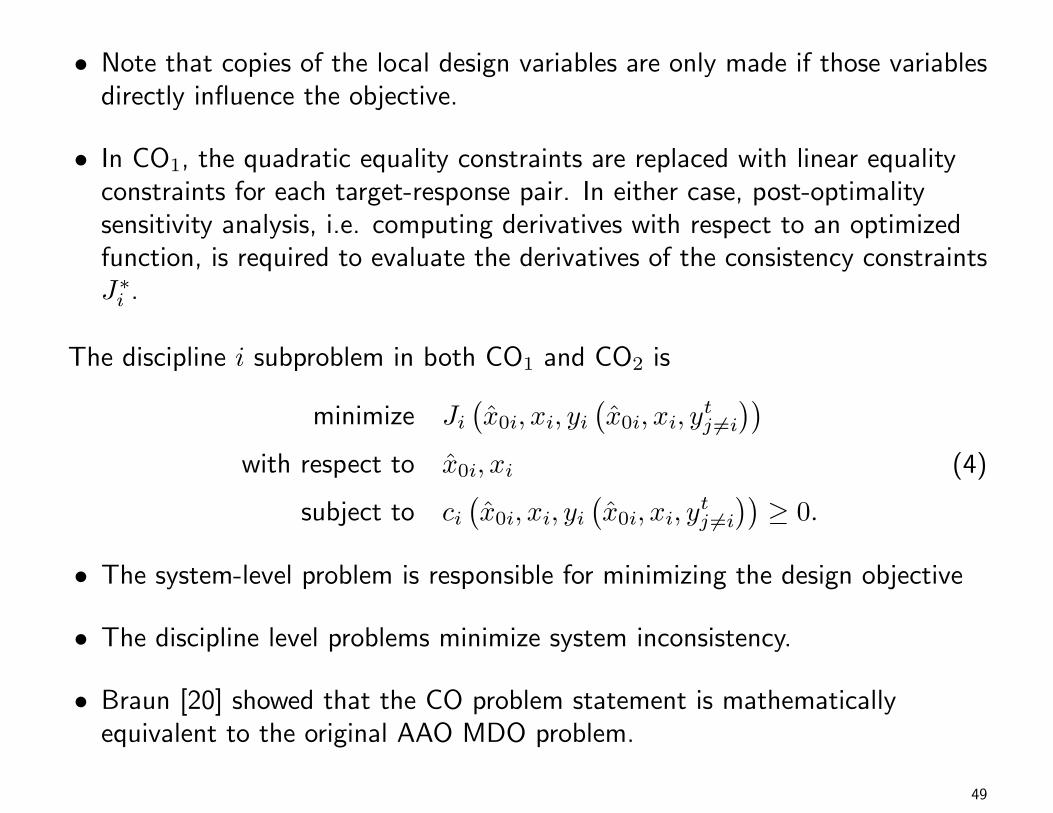
• Note that copies of the local design variables are only made if those variablesdirectly influence the objective.

• In CO1, the quadratic equality constraints are replaced with linear equalityconstraints for each target-response pair. In either case, post-optimalitysensitivity analysis, i.e. computing derivatives with respect to an optimizedfunction, is required to evaluate the derivatives of the consistency constraintsJ∗i .

The discipline i subproblem in both CO1 and CO2 is

minimize Ji(x0i, xi, yi

(x0i, xi, y

tj 6=i

))with respect to x0i, xi

subject to ci(x0i, xi, yi

(x0i, xi, y

tj 6=i

))≥ 0.

(4)

• The system-level problem is responsible for minimizing the design objective

• The discipline level problems minimize system inconsistency.

• Braun [20] showed that the CO problem statement is mathematicallyequivalent to the original AAO MDO problem.

49

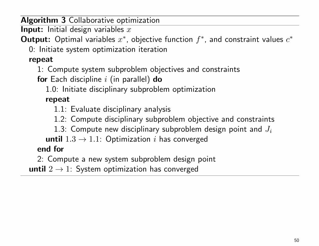
Algorithm 3 Collaborative optimizationInput: Initial design variables xOutput: Optimal variables x∗, objective function f∗, and constraint values c∗

0: Initiate system optimization iterationrepeat

1: Compute system subproblem objectives and constraintsfor Each discipline i (in parallel) do

1.0: Initiate disciplinary subproblem optimizationrepeat

1.1: Evaluate disciplinary analysis1.2: Compute disciplinary subproblem objective and constraints1.3: Compute new disciplinary subproblem design point and Ji

until 1.3→ 1.1: Optimization i has convergedend for2: Compute a new system subproblem design point

until 2→ 1: System optimization has converged

50

In spite of the organizational advantage of having fully separate disciplinarysubproblems, CO has major weaknesses in the mathematical formulation thatlead to poor performance in practice [4, 40].

• In particular, the system problem in CO1 has more equality constraints thanvariables, so if the system cannot be made fully consistent, the systemsubproblem is infeasible. This can also happen in CO2, but it is not the mostproblematic issue.

• The most significant difficulty with CO2 is that the constraint gradients ofthe system problem at an optimal solution are all zero vectors. Thisrepresents a breakdown in the constraint qualification of theKarush–Kuhn–Tucker optimality conditions, which slows down convergencefor most gradient-based optimization software [4]. In the worst case, theCO2 formulation may not converge at all.

These difficulties with the original formulations of CO have inspired severalresearchers to develop modifications to improve the behavior of the architecture.

51

In a few cases, problems have been solved with CO and a gradient-freeoptimizer, such as a genetic algorithm [164], or a gradient-based optimizer thatdoes not use the Lagrange multipliers in the termination condition [96] tohandle the troublesome constraints. While such approaches do avoid theobvious problems with CO, they bring other issues.

• Gradient-free optimizers are computationally expensive and can become thebottleneck within the CO architecture.

• Gradient-based optimizers that do not terminate based on Lagrangemultiplier values, such as feasible direction methods, often fail in nonconvexfeasible regions. As pointed out by DeMiguel [40], the CO systemsubproblem is set-constrained, i.e., nonconvex, because of the need to satisfyoptimality in the disciplinary subproblems.

52

The approach taken by DeMiguel and Murray [40] to fix the problems with COis to relax the troublesome constraints using an L1 exact penalty function witha fixed penalty parameter value and add elastic variables to preserve thesmoothness of the problem. This revised approach is called ModifiedCollaborative Optimization (MCO).

• This approach satisfies the requirement of mathematical rigor, as algorithmsusing the penalty function formulation are known to converge to an optimalsolution under mild assumptions [44, 115].

• However, the test results of Brown and Olds [24] show strange behavior in apractical design problem. In light of their findings, the authors rejected MCOfrom further testing.

53

Another idea, proposed by Sobieski and Kroo [138], uses surrogate models, alsoknown as metamodels, to approximate the post-optimality behavior of thedisciplinary subproblems in the system subproblem.

• This both eliminates the post-optimality sensitivity calculation and improvesthe treatment of the consistency constraints.

• While the approach does seem to be effective for the problems they solve, toour knowledge, it has not been adopted by any other researchers to date.

54

The simplest and most effective known fix for the difficulties of CO involvesrelaxing the system subproblem equality constraints to inequalities with arelaxation tolerance, which was originally proposed by Braun et al. [21].

• This approach was also successful in other test problems [120, 103], wherethe choice of tolerance is a small fixed number, usually 10−6.

• The effectiveness of this approach stems from the fact that a positiveinconsistency value causes the gradient of the constraint to be nonzero if theconstraint is active, eliminating the constraint qualification issue.

• Nonzero inconsistency is not an issue in a practical design setting providedthe inconsistency is small enough such that other errors in the computationalmodel dominate at the final solution.

Li et al. [93] build on this approach by adaptively choosing the tolerance duringthe solution procedure so that the system-level problem remains feasible at eachiteration. This approach appears to work when applied to the test problemsin [4], but has yet to be verified on larger test problems.

55

Despite the numerical issues, CO has been widely implemented on a number ofMDO problems. Most of applications are in the design of aerospace systems.Examples include

1. the design of launch vehicles [23],

2. rocket engines [27],

3. satellite constellations [26],

4. flight trajectories [22, 91],

5. flight control systems [122],

6. preliminary design of complete aircraft [88, 102], and

7. aircraft family design [7].

Outside aerospace engineering, CO has been applied to problems involvingautomobile engines [109], bridge design [9], railway cars [42], and even thedesign of a scanning optical microscope [124].

56

Adaptations of the CO architecture have also been developed for multiobjective,robust, and multifidelity MDO problems. Multiobjective formulations of COwere first described by Tappeta and Renaud [149]. McAllister et al. [110]present a multiobjective approach using linear physical programming. Availablerobust design formulations incorporate the decision-based models of Gu etal. [53] and McAllister and Simpson [109], the implicit uncertainty propagationmethod of Gu et al. [54], and the fuzzy computing models of Huang et al. [68].Multiple model fidelities were integrated into CO for an aircraft design problemby Zadeh and Toropov [163].

57

The most recent version of CO — Enhanced Collaborative Optimization (ECO)— was developed by Roth and Kroo [129, 128]. Figure 10 shows the XDSMcorresponding to this architecture. The problem formulation of ECO, while stillbeing derived from the same basic problem as the original CO architecture, isradically different and therefore deserves additional attention. In a sense, theroles of the system and discipline optimization have been reversed in ECO whencompared to CO. In ECO the system subproblem minimizes system infeasibility,while the disciplinary subproblems minimize the system objective. The systemsubproblem is

minimize J0 =

N∑i=1

||x0i − x0||22 + ||yti − yi(x0, xi, y

tj 6=i

)||22

with respect to x0, yt.

(5)

Note that this subproblem is unconstrained. Also, unlike CO, post-optimalitysensitivities are not required by the system subproblem because the disciplinaryresponses are treated as parameters. The system subproblem chooses theshared design variables by averaging all disciplinary preferences.

58

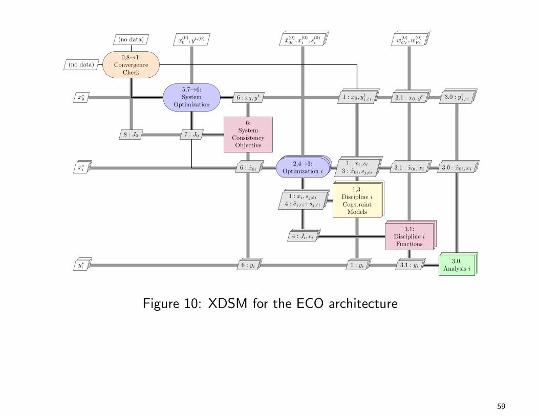
(no data) x(0)0 , yt,(0) x

(0)0i , x

(0)i , s

(0)i w

(0)Ci , w

(0)Fi

(no data)0,8→1:

ConvergenceCheck

x∗0

5,7→6:System

Optimization6 : x0, y

t 1 : x0, ytj 6=i 3.1 : x0, y

t 3.0 : ytj 6=i

8 : J0 7 : J0

6:System

ConsistencyObjective

x∗i 6 : x0i2,4→3:

Optimization i1 : xi, si

3 : x0i, sj 6=i3.1 : x0i, xi 3.0 : x0i, xi

1 : xi, sj 6=i

4 : cj 6=i+sj 6=i

1,3:Discipline iConstraintModels

4 : Ji, ci

3.1:Discipline iFunctions

y∗i 6 : yi 1 : yi 3.1 : yi3.0:

Analysis i

Figure 10: XDSM for the ECO architecture

59

The ith disciplinary subproblem in ECO is

minimize Ji = f0(x0i, yi

(x0i, xi, y

tj 6=i

))+

wCi

(||x0i − x0||22 + ||yti − yi

(x0i, xi, y

tj 6=i

)||22)

+

wFi

N∑j=1,j 6=i

ns∑k=1

sjk

with respect to x0i, xi, sj 6=i

subject to ci(x0i, xi, yi

(x0i, xi, y

tj 6=i

))≥ 0

cj 6=i (x0i)− sj 6=i ≥ 0 j = 1, . . . , N

sj 6=i ≥ 0 j = 1, . . . , N,(6)

where wCi and wFi are penalty weights for the consistency and nonlocal designconstraints, and s is a local set of elastic variables for the constraint models.The wFi penalty weights are chosen to be larger than the largest Lagrangemultiplier, while the wCi weights are chosen to guide the optimization toward aconsistent solution.

60

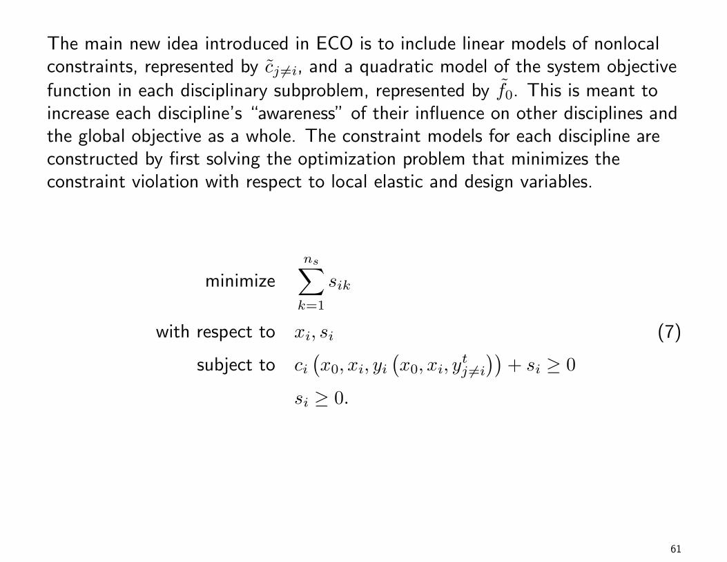
The main new idea introduced in ECO is to include linear models of nonlocalconstraints, represented by cj 6=i, and a quadratic model of the system objective

function in each disciplinary subproblem, represented by f0. This is meant toincrease each discipline’s “awareness” of their influence on other disciplines andthe global objective as a whole. The constraint models for each discipline areconstructed by first solving the optimization problem that minimizes theconstraint violation with respect to local elastic and design variables.

minimizens∑k=1

sik

with respect to xi, si

subject to ci(x0, xi, yi

(x0, xi, y

tj 6=i

))+ si ≥ 0

si ≥ 0.

(7)

61

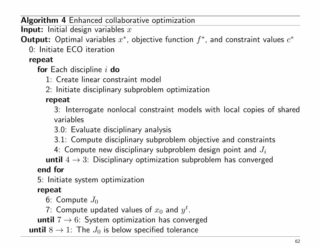
Algorithm 4 Enhanced collaborative optimizationInput: Initial design variables xOutput: Optimal variables x∗, objective function f∗, and constraint values c∗

0: Initiate ECO iterationrepeat

for Each discipline i do1: Create linear constraint model2: Initiate disciplinary subproblem optimizationrepeat

3: Interrogate nonlocal constraint models with local copies of sharedvariables3.0: Evaluate disciplinary analysis3.1: Compute disciplinary subproblem objective and constraints4: Compute new disciplinary subproblem design point and Ji

until 4→ 3: Disciplinary optimization subproblem has convergedend for5: Initiate system optimizationrepeat

6: Compute J07: Compute updated values of x0 and yt.

until 7→ 6: System optimization has convergeduntil 8→ 1: The J0 is below specified tolerance

62

Based on the Roth’s results [129, 128], ECO is effective in reducing the numberof discipline analyses compared to CO. The trade-off is in the additional timerequired to build and update the models for each discipline, weighed against thesimplified solution to the decomposed optimization problems. The results alsoshow that ECO compares favorably with the Analytical Target Cascadingarchitecture (which we will describe in Section 4.5).

While ECO seems to be effective, CO tends to be an inefficient architecture forsolving MDO problems.

• Without any of the fixes discussed in this section, the architecture alwaysrequires a disproportionately large number of function and disciplineevaluations [79, 83, 37, 162], assuming it converges at all.

• When the system-level equality constraints are relaxed, the results from COare more competitive with other distributed architectures [121, 103, 150] butstill compare poorly with the results of monolithic architectures.

63

4.4 Bilevel Integrated System Synthesis (BLISS)

The BLISS architecture [143], like CSSO, is a method for decomposing theMDF problem along disciplinary lines.

• Unlike CSSO, however, BLISS assigns local design variables to disciplinarysubproblems and shared design variables to the system subproblem.

• The basic approach of the architecture is to form a path in the design spaceusing a series of linear approximations to the original design problem, withuser-defined bounds on the design variable steps, to prevent the design pointfrom moving so far away that the approximations are too inaccurate.

This is an idea similar to that of trust-region methods [34]. Theseapproximations are constructed at each iteration using global sensitivityinformation.

64

The BLISS system level subproblem is formulated as

minimize (f∗0 )0 +

(df∗0dx0

)∆x0

with respect to ∆x0

subject to (c∗0)0 +

(dc∗0dx0

)∆x0 ≥ 0

(c∗i )0 +

(dc∗idx0

)∆x0 ≥ 0 for i = 1, . . . , N

∆x0L ≤ ∆x0 ≤ ∆x0U .

(8)

65

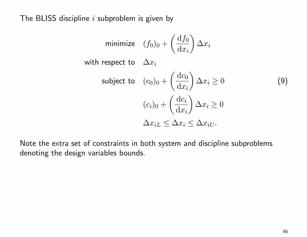
The BLISS discipline i subproblem is given by

minimize (f0)0 +

(df0dxi

)∆xi

with respect to ∆xi

subject to (c0)0 +

(dc0dxi

)∆xi ≥ 0

(ci)0 +

(dcidxi

)∆xi ≥ 0

∆xiL ≤ ∆xi ≤ ∆xiU .

(9)

Note the extra set of constraints in both system and discipline subproblemsdenoting the design variables bounds.

66

x(0) yt,(0) x(0)0 x

(0)i

(no data)0,11→1:

ConvergenceCheck

1,3→2:MDA

6 : ytj 6=i 6, 9 : ytj 6=i 6 : ytj 6=i 2, 5 : ytj 6=i

x∗0 11 : x0

8,10:System

Optimization6, 9 : x0 6, 9 : x0 9 : x0 6 : x0 2, 5 : x0

x∗i 11 : xi4,7:

Optimization i6, 9 : xi 6, 9 : xi 9 : xi 6 : xi 2, 5 : xi

10 : f0, c0 7 : f0, c0

6,9:System

Functions

10 : fi, ci 7 : fi, ci

6,9:Discipline iFunctions

10 : df/dx0, dc/dx0

9:SharedVariable

Derivatives

7 : df0,i/ dxi, dc0,i/ dxi

6:Discipline iVariable

Derivatives

y∗i 3 : yi 6, 9 : yi 6, 9 : yi 9 : yi 6 : yi2,5:

Analysis i

Figure 11: Diagram for the BLISS architecture

67

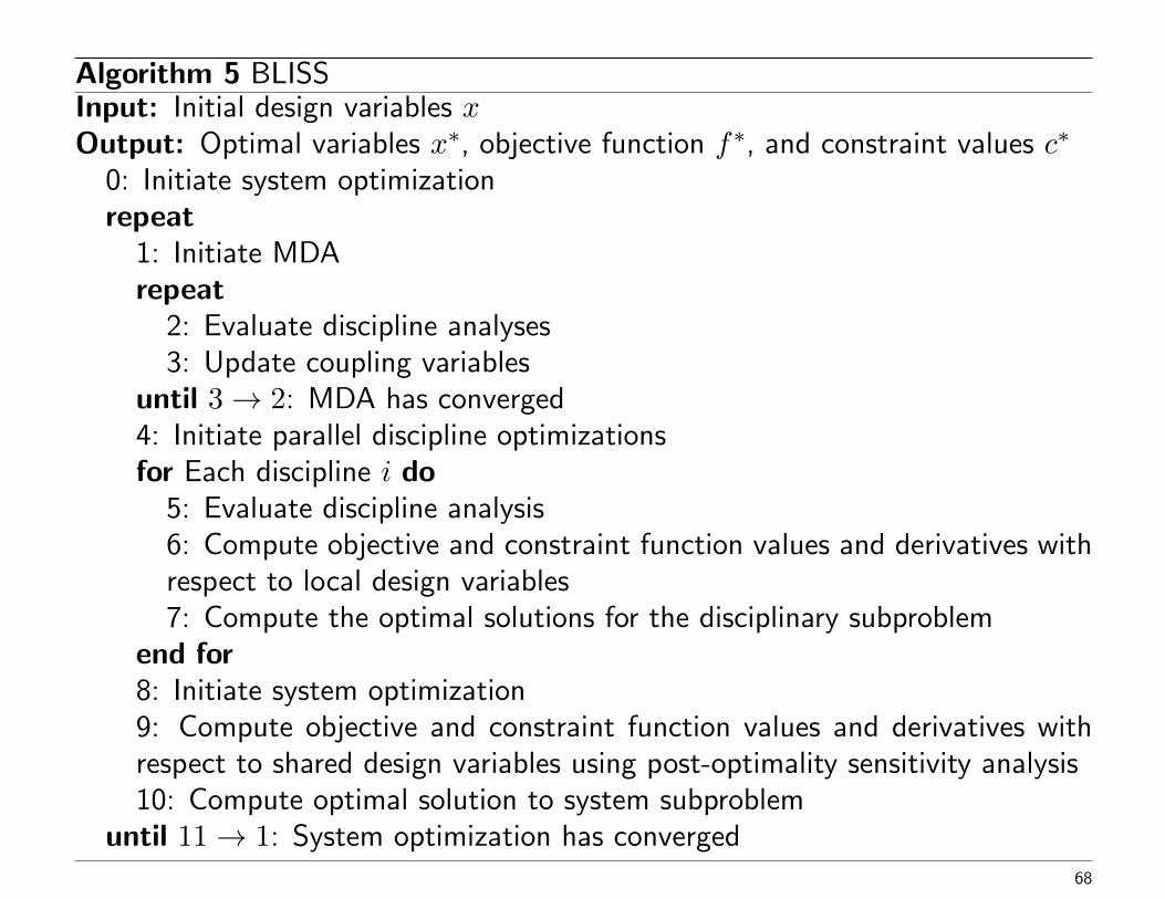
Algorithm 5 BLISSInput: Initial design variables xOutput: Optimal variables x∗, objective function f∗, and constraint values c∗

0: Initiate system optimizationrepeat

1: Initiate MDArepeat

2: Evaluate discipline analyses3: Update coupling variables

until 3→ 2: MDA has converged4: Initiate parallel discipline optimizationsfor Each discipline i do

5: Evaluate discipline analysis6: Compute objective and constraint function values and derivatives withrespect to local design variables7: Compute the optimal solutions for the disciplinary subproblem

end for8: Initiate system optimization9: Compute objective and constraint function values and derivatives withrespect to shared design variables using post-optimality sensitivity analysis10: Compute optimal solution to system subproblem

until 11→ 1: System optimization has converged68

In order to prevent violation of the disciplinary constraints by changes in theshared design variables, post-optimality sensitivity information is required tosolve the system subproblem.

For this step, Sobieski [143] presents two methods:

BLISS/A: using a generalized version of the Global Sensitivity Equations [140],and

BLISS/B: using the “pricing” interpretation of local Lagrange multipliers.

Other variations use response surface approximations to computepost-optimality sensitivity data [81, 73].

69

Some notes on the BLISS algorithm:

• due to the linear nature of the optimization problems under consideration,repeated interrogation of the objective and constraint functions is notnecessary once gradient information is available.

• However, this reliance on linear approximations is not without difficulties. Ifthe underlying problem is highly nonlinear, the algorithm may convergeslowly. The presence of user-defined variable bounds may help theconvergence if these bounds are properly chosen, such as through a trustregion framework.

• Detailed knowledge of the design space can also help, but this increases theoverhead cost of implementation.

70

Two other adaptations of the original BLISS architecture are known in theliterature.

1. The first is Ahn and Kwon’s proBLISS [2], an architecture forreliability-based MDO. Their results show that the architecture is competitivewith reliability-based adaptations of MDF and IDF.

2. The second is LeGresley and Alonso’s BLISS/POD [92], an architecture thatintegrates a reduced-order modeling technique called Proper OrthogonalDecomposition [13] to reduce the cost of the multidisciplinary analysis andsensitivity analysis steps. Their results show a significant improvement in theperformance of BLISS, to the point where it is almost competitive with MDF.

71

As an enhancement of the original BLISS, a radically different formulationcalled BLISS-2000 was developed by Sobieski et al. [144].

• BLISS-2000 does not require a multidisciplinary analysis to restore feasibilityof the design, so we have separated it from other BLISS variants in theclassification tree shown earlier.

• like other IDF-derived architectures, BLISS-2000 uses coupling variabletargets to enforce consistency at the optimum. Information exchangebetween system and discipline subproblems is completed through surrogatemodels of the disciplinary optima.

72

The BLISS-2000 system subproblem is given by

minimize f0(x, y

(x, yt

))with respect to x0, y

t, w

subject to c0(x, y

(x, yt, w

))≥ 0

yti − yi(x0, xi, y

tj 6=i, wi

)= 0 for i = 1, . . . , N.

(10)

The BLISS-2000 discipline i subproblem is

minimize wTi yi

with respect to xi

subject to ci(x0, xi, yi

(x0, xi, y

tj 6=i

))≥ 0.

(11)

A unique aspect of this architecture is the use of a vector of weightingcoefficients, wi, attached to the disciplinary states. These weighting coefficientsgive the user a measure of control over state variable preferences. Generallyspeaking, the coefficients should be chosen based on the structure of the globalobjective to allow disciplinary subproblems to find an optimum more quickly.How much the choice of coefficients affects convergence has yet to bedetermined.

73

x(0)0 x

(0)0 , yt,(0), w(0) x

(0)0 , y

t,(0)j 6=i , w

(0)i x

(0)i

(no data)0,12→1:

ConvergenceCheck

x∗0, w∗ 12 : x0

8,11→9:System

Optimization10 : x0, y

t 9 : x0, ytj 6=i, wi 1 : x0, y

tj 6=i, wi

11 : f0, c0, cc

10:System

Functions

x∗i , y∗i 10 : xi, yi

6,9Metamodel i

6 : x0, ytj 6=i, wi

1,7→2:DOE i

4 : x0, wi 3 : x0, ytj 6=i

6 : xi2,5→3:

Optimization i4 : xi 3 : xi

5 : fi, ci

4:Discipline iFunctions

6 : yi 4 : yi3:

Analysis i

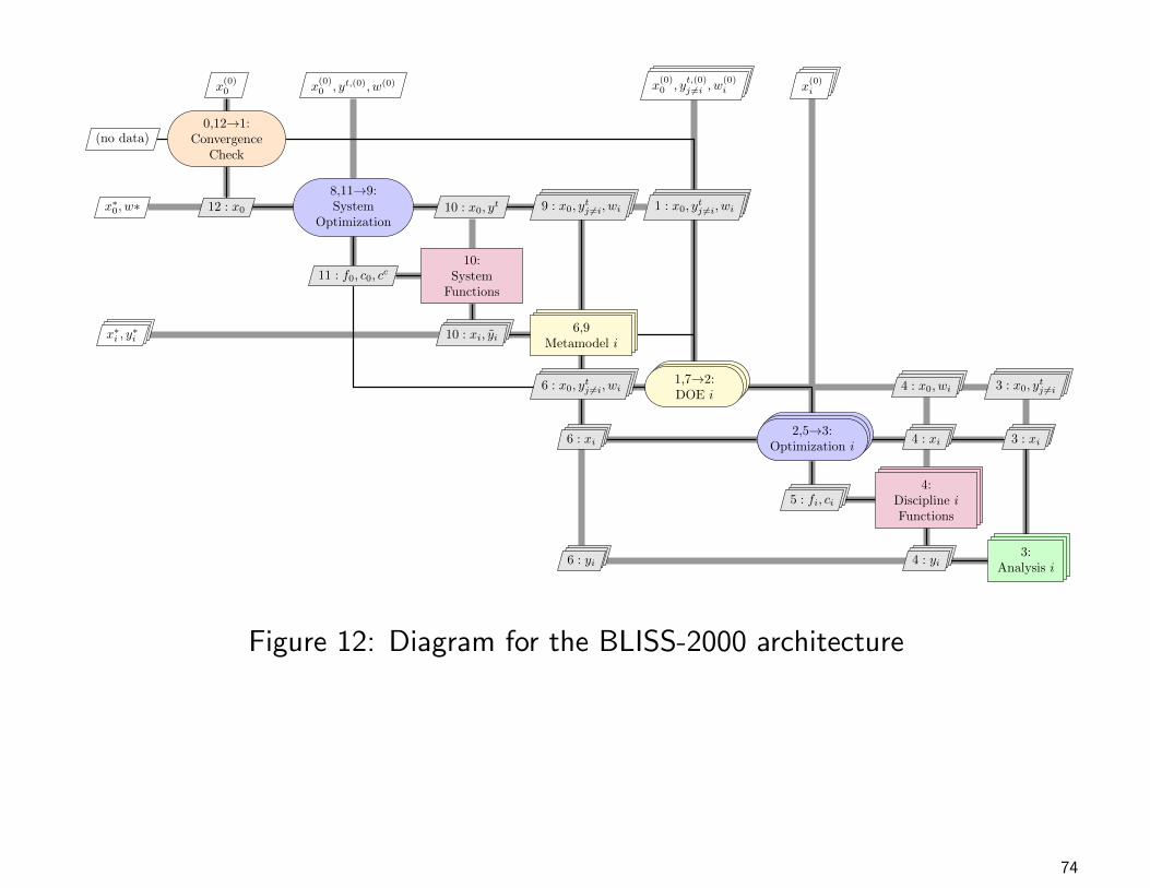
Figure 12: Diagram for the BLISS-2000 architecture

74

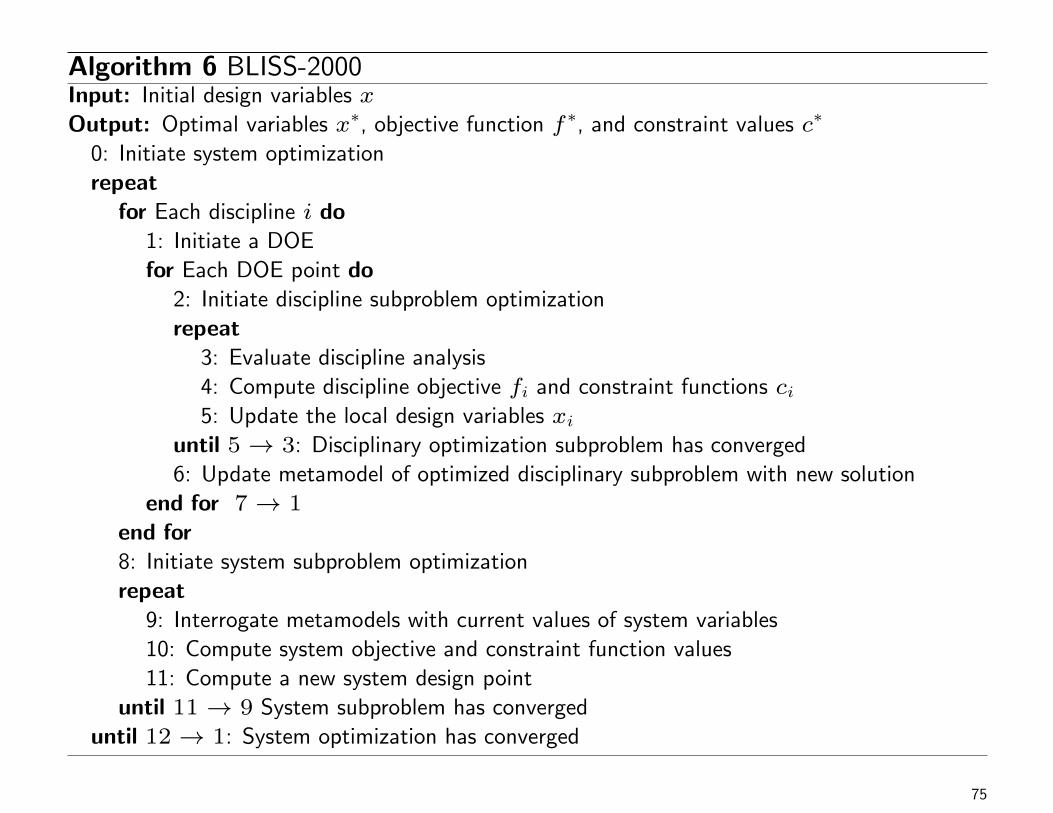
Algorithm 6 BLISS-2000Input: Initial design variables x

Output: Optimal variables x∗, objective function f∗, and constraint values c∗

0: Initiate system optimization

repeatfor Each discipline i do

1: Initiate a DOE

for Each DOE point do2: Initiate discipline subproblem optimization

repeat3: Evaluate discipline analysis

4: Compute discipline objective fi and constraint functions ci5: Update the local design variables xi

until 5→ 3: Disciplinary optimization subproblem has converged

6: Update metamodel of optimized disciplinary subproblem with new solution

end for 7→ 1

end for8: Initiate system subproblem optimization

repeat9: Interrogate metamodels with current values of system variables

10: Compute system objective and constraint function values

11: Compute a new system design point

until 11→ 9 System subproblem has converged

until 12→ 1: System optimization has converged

75

A unique aspect of this architecture is the use of a vector of weightingcoefficients, wi, attached to the disciplinary states. These weighting coefficientsgive the user a measure of control over state variable preferences.

• the coefficients should be chosen based on the structure of the globalobjective to allow disciplinary subproblems to find an optimum more quickly

• How much the choice of coefficients affects convergence has yet to bedetermined.

76

BLISS-2000 possesses several advantages over the original BLISS architecture.

1. the solution procedure is much easier to understand.

2. the decomposed problem formulation of BLISS-2000 is equivalent to theAAO problem we want to solve [144].

3. by using metamodels for each discipline, rather than for the whole system,the calculations for BLISS-2000 can be run in parallel with minimalcommunication between disciplines.

4. BLISS-2000 seems to be more flexible than its predecessor.

Recently, Sobieski detailed an extension of BLISS-2000 to handle multilevel,system-of-systems problems [142]. In spite of these advantages, it appears thatBLISS-2000 has not been used nearly as frequently as the original BLISSformulation.

77

4.5 Analytical Target Cascading (ATC)

The ATC architecture was not initially developed as an MDO architecture, butas a method to propagate system targets — i.e., requirements or desirableproperties — through a hierarchical system to achieve a feasible system designsatisfying these targets [74, 77].

• If the system targets were unattainable, the ATC architecture would return adesign point minimizing the inattainability.

• Effectively, the ATC architecture is no different from an MDO architecturewith a system objective of minimizing the squared difference between a set ofsystem targets and model responses.

• By simply changing the objective function, we can solve general MDOproblems using ATC.

78

The ATC problem formulation that we present here is due to Tosserams etal. [153]:

minimize f0(x, yt

)+

N∑i=1

Φi

(x0i − x0, yti − yi

(x0, xi, y

t))

+

Φ0

(c0(x, yt

))with respect to x0, y

t,

(12)

where Φ0 is a penalty relaxation of the global design constraints and Φi is apenalty relaxation of the discipline i consistency constraints. The ith disciplinesubproblem is:

minimize f0(x0i, xi, yi

(x0i, xi, y

tj 6=i

), ytj 6=i

)+ fi

(x0i, xi, yi

(x0i, xi, y

tj 6=i

))+

Φi

(yti − yi

(x0i, xi, y

tj 6=i

), x0i − x0

)+

Φ0

(c0(x0i, xi, yi

(x0i, xi, y

tj 6=i

), ytj 6=i

))with respect to x0i, xi

subject to ci(x0i, xi, yi

(x0i, xi, y

tj 6=i

))≥ 0.

(13)

79

w(0) x(0)0 , yt,(0) x

(0)0i , x

(0)i

(no data)0,8→1:

w update6 : w 3 : wi

x∗0

5,7→6:System

Optimization6 : x0, y

t 3 : x0, yt 2 : ytj 6=i

7 : f0,Φ0···N

6:System and

PenaltyFunctions

x∗i 6 : x0i, xi1,4→2:

Optimization i3 : x0i, xi 2 : x0i, xi

4 : fi, ci,Φ0,Φi

3:Discipline iand PenaltyFunctions

y∗i 6 : yi 3 : yi2:

Analysis i

Figure 13: Diagram for the ATC architecture

80

Algorithm 7 ATCInput: Initial design variables xOutput: Optimal variables x∗, objective function f∗, and constraint values c∗

0: Initiate main ATC iterationrepeat

for Each discipline i do1: Initiate discipline optimizerrepeat

2: Evaluate disciplinary analysis3: Compute discipline objective and constraint functions and penaltyfunction values4: Update discipline design variables

until 4→ 2: Discipline optimization has convergedend for5: Initiate system optimizerrepeat

6: Compute system objective, constraints, and all penalty functions7: Update system design variables and coupling targets.

until 7→ 6: System optimization has converged8: Update penalty weights

until 8→ 1: Penalty weights are large enough

81

Note that ATC can be applied to a multilevel hierarchy of systems just as wellas a discipline-based non-hierarchic system.

• In the multilevel case, the penalty functions are applied to all constraintsthat combine local information with information from the levels immediatelyabove or below the current one.

• Also note that post-optimality sensitivity data is not needed in any of thesubproblems as nonlocal data are always treated as fixed values in thecurrent subproblem.

82

The most common penalty functions in ATC are quadratic penalty functions.

• The proper selection of the penalty weights is important for both finalinconsistency in the discipline models and convergence of the algorithm.

• Michalek and Papalambros [112] present an effective weight update methodthat is especially useful when unattainable targets have been set in atraditional ATC process.

• Michelena et al. [114] present several coordination algorithms using ATC withquadratic penalty functions and demonstrate the convergence for all of them.

Note that, as with penalty methods for general optimization problems, (see,e.g., Nocedal and Wright [115, chap. 17]) the solution of the MDO problemmust be computed to reasonable accuracy before the penalty weights areupdated. However, because we are now dealing with a distributed set ofsubproblems, the whole hierarchy of subproblems must be solved for a given setof weights. This is due to the nonseparable nature of the quadratic penaltyfunction.

83

Several other penalty function choices and associated coordination approacheshave also been devised for ATC.

1. Kim et al. [75] outline a version of ATC that uses Lagrangian relaxation anda sub-gradient method to update the multiplier estimates.

2. Tosserams et al. [151] use augmented Lagrangian relaxation with Bertsekas’method of multipliers [14] and alternating direction method ofmultipliers [15] to update the penalty weights. They also group this variantof ATC into a larger class of coordination algorithms known as AugmentedLagrangian Coordination [153].

3. Li et al. [94] apply the diagonal quadratic approximation approach ofRuszcynski [130] to the augmented Lagrangian to eliminate subproblemcoupling through the quadratic terms and further parallelize the architecture.

4. Han and Papalambros [62] propose a version of ATC based on sequentiallinear programming [11, 28], where inconsistency is penalized using infinitynorms. They later presented a convergence proof of this approach in a shortnote [61].

84

For each of the above penalty function choices, ATC was able to produce thesame design solutions as the monolithic architectures.

85

Despite having been developed relatively recently, the ATC architecture hasbeen widely used. By far, ATC has been most frequently applied to designproblems in the field for which it was developed, the automotiveindustry [84, 76, 78, 19, 85, 147, 29, 63].

• However, the ATC approach has also proven to be useful in aircraftdesign [8, 7, 158] and building design [32].

• ATC has also found applications outside of strict engineering designproblems, including manufacturing decisions [95], supply chainmanagement [67], and marketing decisions in product design [111].

• Huang et al. [66] have developed an ATC-specific web portal to solveoptimization problems via the ATC architecture. Etman et al. [43] discussthe automatic implementation of coordination procedures, using ATC as anexample architecture.

• There are ATC formulations that can handle integer variables [113] andprobabilistic design problems [86, 98].

• Another important adaptation of ATC applies to problems with

86

block-separable linking constraints [155]. In this class of problems, c0consists of constraints which are sums of functions depending on only sharedvariables and the local variables of one discipline.

87

The performance of ATC compared with other architectures is not well knownbecause only one result is available.

• In de Wit and Van Keulen’s architecture comparison [37], ATC is competitivewith all other benchmarked distributed architectures, including standardversions of CSSO, CO, and BLISS.

• However, ATC and the other distributed architectures are not competitivewith a monolithic architecture in terms of the number of function anddiscipline evaluations.

More commonly, different versions of ATC are benchmarked against each other.

• Tosserams et al. [151] compared the augmented Lagrangian penaltyapproach with the quadratic penalty approach and found much improvedresults with the alternating direction method of multipliers.

• Surprisingly, de Wit and van Keulen [37] found the augmented Lagrangianversion performed worse than the quadratic penalty method for their testproblem.

88

• Han and Papalambros [62] compared their sequential linear programmingversion of ATC to several other approaches and found a significant reductionin the number of function evaluations. However, they note that thecoordination overhead is large compared to other ATC versions and stillneeds to be addressed.

89

4.6 Exact and Inexact Penalty Decomposition (EPD andIPD)

If there are no system-wide constraints or objectives, i.e., if neither f0 and c0exist, the Exact or Inexact Penalty Decompositions (EPD or IPD) [39, 41] maybe employed. Both formulations rely on solving the disciplinary subproblem

minimize fi(x0i, xi, yi

(x0i, xi, y

tj 6=i

))+ Φi

(x0i − x0, yti − yi

(x0i, xi, y

tj 6=i

))with respect to x0i, xi

subject to ci(x0i, xi, yi

(x0i, xi, y

tj 6=i

))≥ 0.

(14)

Here, Φi denotes the penalty function associated with the inconsistencybetween the ith disciplinary information and the system information. In EPD,Φi is an L1 penalty function with additional variables and constraints added toensure smoothness. In IPD, Φi is a quadratic penalty function with appropriatepenalty weights. The notation x0i denotes a local copy of the shared designvariables in discipline i, while x0 denotes the system copy.

90

w(0) x(0)0 , yt,(0) x

(0)0i , x

(0)i

(no data)0,8→1:

w update3, 6 : wi

x∗0

5,7→6:System

Optimization3, 6 : x0, y

t 2 : ytj 6=i

x∗i1,4→2:

Optimization i3, 6 : x0i 3 : x0i, xi 2 : x0i, xi

7 : Φi 4 : Φi

3,6:Penalty

Function i

4 : fi, ci

3:Discipline iFunctions

y∗i 3, 6 : yi 3 : yi2:

Analysis i

Figure 14: Diagram for the penalty decomposition architectures EPD and IPD

91

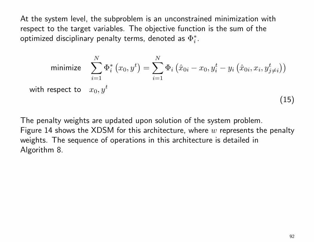
At the system level, the subproblem is an unconstrained minimization withrespect to the target variables. The objective function is the sum of theoptimized disciplinary penalty terms, denoted as Φ∗i .

minimizeN∑i=1

Φ∗i(x0, y

t)

=

N∑i=1

Φi

(x0i − x0, yti − yi

(x0i, xi, y

tj 6=i

))with respect to x0, y

t

(15)

The penalty weights are updated upon solution of the system problem.Figure 14 shows the XDSM for this architecture, where w represents the penaltyweights. The sequence of operations in this architecture is detailed inAlgorithm 8.

92

Algorithm 8 EPD and IPDInput: Initial design variables xOutput: Optimal variables x∗, objective function f∗, and constraint values c∗

0: Initiate main iterationrepeat

for Each discipline i dorepeat

1: Initiate discipline optimizer2: Evaluate discipline analysis3: Compute discipline objective and constraint functions, and penaltyfunction values4: Update discipline design variables

until 4→ 2: Discipline optimization has convergedend for5: Initiate system optimizerrepeat

6: Compute all penalty functions7: Update system design variables and coupling targets

until 7→ 6: System optimization has converged8: Update penalty weights.

until 8→ 1: Penalty weights are large enough

93

Both EPD and IPD have mathematically provable convergence under the linearindependence constraint qualification and with mild assumptions on the updatestrategy for the penalty weights [41].

• In particular, the penalty weight in IPD must monotonically increase until theinconsistency is sufficiently small, similar to other quadratic penaltymethods [115].

• For EPD, the penalty weight must be larger than the largest Lagrangemultiplier, following established theory of the L1 penalty function [115],while the barrier parameter must monotonically decrease like in an interiorpoint method [160].

• If other penalty functions are employed, the parameter values are selectedand updated according to the corresponding mathematical theory.

Under these conditions, the solution obtained under EPD and IPD will also be asolution to the desired AAO MDO problem.

94

Only once in the literature has either penalty decomposition architecture beentested against any others.

• The results of Tosserams et al. [152] suggest that performance depends onthe choice of penalty function employed.

• A comparison between IPD with a quadratic penalty function and IPD withan augmented Lagrangian penalty function showed that the lattersignificantly outperformed the former in terms of both time and number offunction evaluations on several test problems.

95

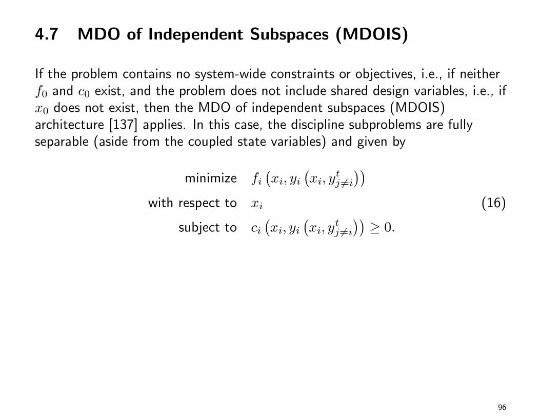
4.7 MDO of Independent Subspaces (MDOIS)

If the problem contains no system-wide constraints or objectives, i.e., if neitherf0 and c0 exist, and the problem does not include shared design variables, i.e., ifx0 does not exist, then the MDO of independent subspaces (MDOIS)architecture [137] applies. In this case, the discipline subproblems are fullyseparable (aside from the coupled state variables) and given by

minimize fi(xi, yi

(xi, y

tj 6=i

))with respect to xi

subject to ci(xi, yi

(xi, y

tj 6=i

))≥ 0.

(16)

96

x(0) yt,(0) x(0)i

(no data)0,8→1:

ConvergenceCheck

1,3→2:MDA

6 : ytj 6=i 2, 5 : ytj 6=i

x∗i 8 : xi4,7→5:

Optimization i6 : xi 2, 5 : xi

7 : fi, ci

6:Discipline iFunctions

y∗i 3 : yi 6 : yi2,5:

Analysis i

Figure 15: Diagram for the MDOIS architecture

97

Algorithm 9 MDOISInput: Initial design variables xOutput: Optimal variables x∗, objective function f∗, and constraint values c∗

0: Initiate main iterationrepeat

repeat1: Initiate MDA2: Evaluate discipline analyses3: Update coupling variables

until 3→ 2: MDA has convergedfor Each discipline i do

4: Initiate disciplinary optimizationrepeat

5: Evaluate discipline analysis6: Compute discipline objectives and constraints7: Compute a new discipline design point

until 7→ 5: Discipline optimization has convergedend for

until 8→ 1 Main iteration has converged

98

Some notes on MDOIS:

• The targets are just local copies of system state information.

• Upon solution of the disciplinary problems, which can access the output ofindividual disciplinary analysis codes, a full multidisciplinary analysis iscompleted to update all target values. Thus, rather than a systemsubproblem used by other architectures, the MDA is used to guide thedisciplinary subproblems to a design solution.

• Shin and Park [137] show that under the given problem assumptions anoptimal design is found using this architecture.

Benchmarking results are available comparing MDOIS to some of the olderarchitectures. These results are given by Yi et al. [162].

• In many cases, MDOIS requires fewer analysis calls than MDF while stillbeing able to reach the optimal solution.

• However, MDOIS still does not converge as fast as IDF and the restrictive

99

definition of the problem means that the architecture is not nearly as flexibleas MDF.

• A practical problem that can be solved using MDOIS is the belt-integratedseat problem of Shin et al. [136]. However, the results using MDOIS havenot been compared to results obtained using other architectures.

100

4.8 Quasiseparable Decomposition (QSD)

Haftka and Watson [59] developed the QSD architecture to solve quasiseparableoptimization problems.

• In a quasiseparable problem, the system objective and constraint functionsare assumed to be dependent only on global variables (i.e., the shared designand coupling variables).

• This type of problem may be thought of as identical to the complicatingvariables problems.

We have not come across any practical design problems that satisfy thisproperty. However, if required by the problem, we can easily transform thegeneral (AAO) MDO problem into a quasiseparable problem.

• This is accomplished by duplicating the relevant local variables, and forcingthe global objective to depend on the target copies of local variables.

• The resulting quasiseparable problem and decomposition is mathematicallyequivalent to the original problem.

101

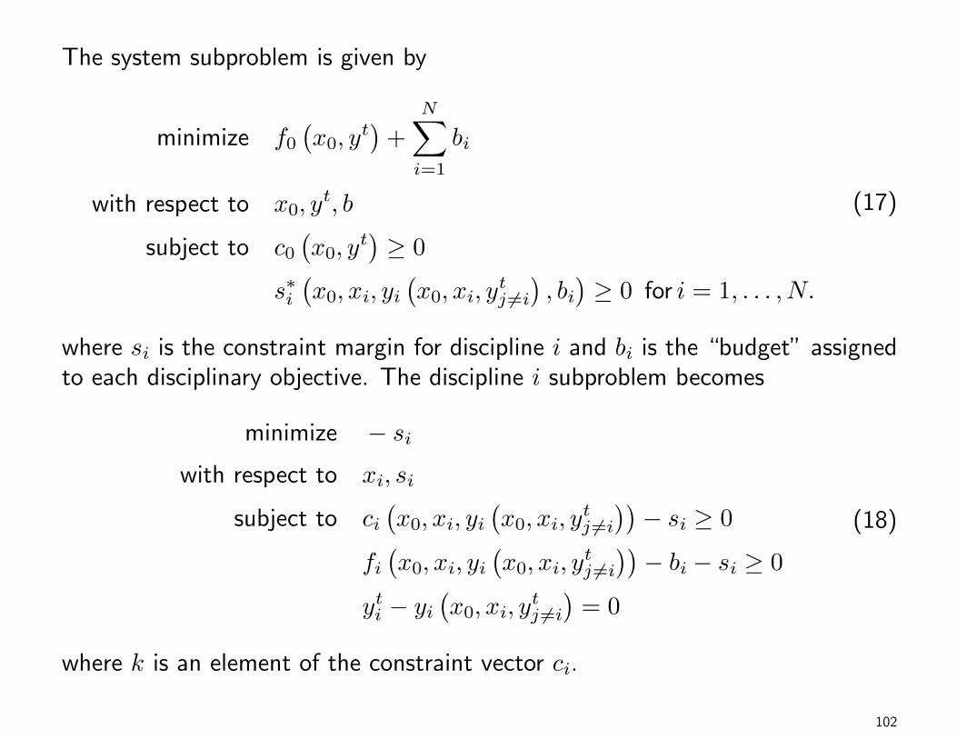
The system subproblem is given by

minimize f0(x0, y

t)

+

N∑i=1

bi

with respect to x0, yt, b

subject to c0(x0, y

t)≥ 0

s∗i(x0, xi, yi

(x0, xi, y

tj 6=i

), bi)≥ 0 for i = 1, . . . , N.

(17)

where si is the constraint margin for discipline i and bi is the “budget” assignedto each disciplinary objective. The discipline i subproblem becomes

minimize − siwith respect to xi, si

subject to ci(x0, xi, yi

(x0, xi, y

tj 6=i

))− si ≥ 0

fi(x0, xi, yi

(x0, xi, y

tj 6=i

))− bi − si ≥ 0

yti − yi(x0, xi, y

tj 6=i

)= 0

(18)

where k is an element of the constraint vector ci.

102

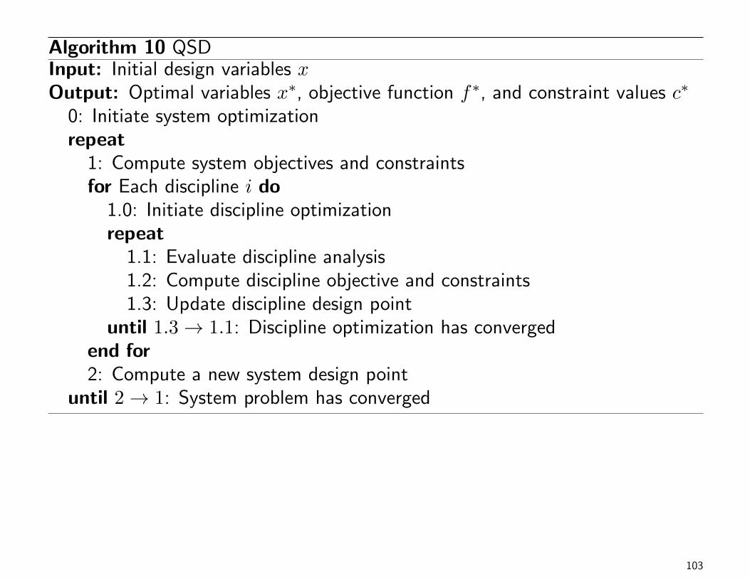
Algorithm 10 QSDInput: Initial design variables xOutput: Optimal variables x∗, objective function f∗, and constraint values c∗

0: Initiate system optimizationrepeat

1: Compute system objectives and constraintsfor Each discipline i do

1.0: Initiate discipline optimizationrepeat

1.1: Evaluate discipline analysis1.2: Compute discipline objective and constraints1.3: Update discipline design point

until 1.3→ 1.1: Discipline optimization has convergedend for2: Compute a new system design point

until 2→ 1: System problem has converged

103

x(0)0 , yt,(0), b(0) x

(0)i , s

(0)i

x∗0

0,2→1:System

Optimization1 : x0, y

t 1.2 : x0, yt, bi 1.1 : x0, y

tj 6=i

2 : f0, c0

1:System

Functions

x∗i 2 : s∗i1.0,1.3→1.1:

Optimization i1.2 : xi, si 1.1 : xi

1.3 : fi, ci, cci

1.2Discipline iFunctions

y∗i 1.2 : yi1.1

Analysis i

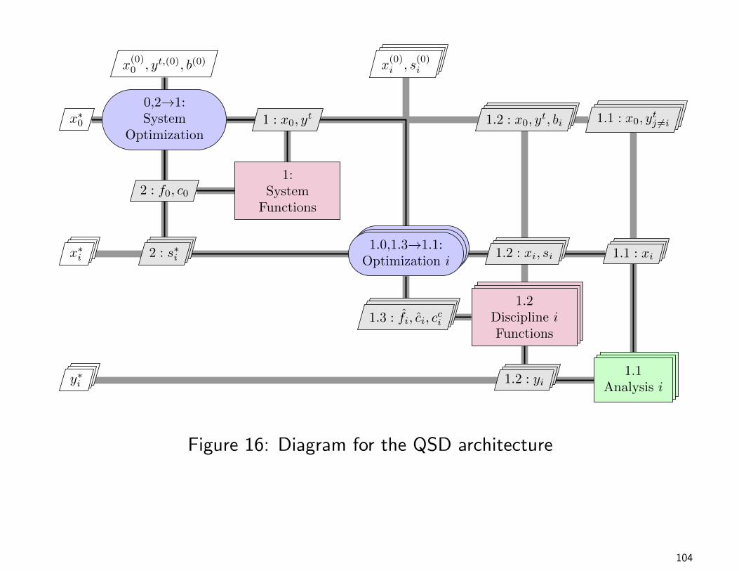
Figure 16: Diagram for the QSD architecture

104

Some notes on QSD:

• Due to the use of target copies, we classify this architecture as distributedIDF.

• This is a bilevel architecture where the solutions of disciplinary subproblemsare constraints in the system subproblem. Therefore, post-optimalitysensitivities or surrogate model approximations of optimized disciplinarysubproblems are required to solve the system subproblem.

• Haftka and Watson have extended the theory behind QSD to solve problemswith a combination of discrete and continuous variables [60].

• Liu et al. [97] successfully applied QSD with surrogate models to a structuraloptimization problem. However, they made no comparison of theperformance to other architectures, not even QSD without the surrogates.

• A version of QSD without surrogate models was benchmarked by de Wit andvan Keulen [37]. Unfortunately, this architecture was the worst of all thearchitectures tested in terms of disciplinary evaluations.

105

A version of QSD using surrogate models should yield improved performance,due to the smoothness introduced by the model, but this version has not beenbenchmarked to our knowledge.

106

4.9 Asymmetric Subspace Optimization (ASO)

The ASO architecture [31] is a new distributed-MDF architecture.

• It was motivated by the case of high-fidelity aerostructural optimization,where the aerodynamic analysis typically requires an order of magnitudemore time to complete than the structural analysis [105].

• To reduce the number of expensive aerodynamic analyses, the structuralanalysis is coupled with a structural optimization inside the MDA.

• This idea can be readily generalized to any problem where there is a widediscrepancy between discipline analysis times.

107

The system subproblem in ASO is

minimize f0 (x, y (x, y)) +∑k

fk (x0, xk, yk (x0, xk, yj 6=k))

with respect to x0, xk

subject to c0 (x, y (x, y)) ≥ 0

ck (x0, xk, yk (x0, xk, yj 6=k)) ≥ 0 for all k,(19)

where subscript k denotes disciplinary information that remains outside of theMDA. The disciplinary problem for discipline i, which is resolved inside theMDA, is

minimize f0 (x, y (x, y)) + fi (x0, xi, yi (x0, xi, yj 6=i))

with respect to xi

subject to ci (x0, xi, yi (x0, xi, yj 6=i)) ≥ 0.

(20)

108

x(0)0,1,2 yt,(0) x

(0)3

x∗0,1,2

0,10→1:System

Optimization9 : x0,1,2 2 : x0, x1 3 : x0, x2 6 : x0,1,2 5 : x0

10 : f0,1,2, c0,1,2

9:Discipline 0, 1,

and 2Functions

1,8→2:MDA

2 : yt2, yt3 3 : yt3

y∗1 9 : y1 8 : y12:

Analysis 13 : y1 6 : y1 5 : y1

y∗2 9 : y2 8 : y23:

Analysis 26 : y2 5 : y2

x∗3 9 : x3

4,7→5:Optimization 3

6 : x3 5 : x3

7 : f0, c0, f3, c3

6:Discipline 0

and 3Functions

y∗3 9 : y3 8 : y3 6 : y35:

Analysis 3

Figure 17: Diagram for the ASO architecture

109

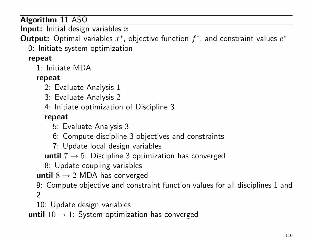
Algorithm 11 ASOInput: Initial design variables xOutput: Optimal variables x∗, objective function f∗, and constraint values c∗

0: Initiate system optimizationrepeat

1: Initiate MDArepeat

2: Evaluate Analysis 13: Evaluate Analysis 24: Initiate optimization of Discipline 3repeat

5: Evaluate Analysis 36: Compute discipline 3 objectives and constraints7: Update local design variables

until 7→ 5: Discipline 3 optimization has converged8: Update coupling variables

until 8→ 2 MDA has converged9: Compute objective and constraint function values for all disciplines 1 and210: Update design variables

until 10→ 1: System optimization has converged

110

Notes on ASO:

• The optimality of the final solution is preserved by using the coupledpost-optimality sensitivity (CPOS) equations, developed by Chittick andMartins [31], to calculate gradients at the system level.

• CPOS represents the extension of the coupled sensitivity equations [141, 106]to include the optimality conditions.

• ASO was later implemented using a coupled-adjoint approach as well [30].

• Kennedy et al. [72] present alternative strategies for computing thedisciplinary subproblem optima and the post-optimality sensitivity analysis.

• As with other bilevel MDO architectures, the post-optimality analysis isnecessary to ensure convergence to an optimal design of the originalmonolithic problem.

111

Results of ASO show a substantial reduction in the number of calls to theaerodynamics analysis, and even a slight reduction in the number of calls to thestructural analysis [31].

• However, the total time for the optimization routine is only competitive withMDF if the aerodynamic analysis is substantially more costly than thestructural analysis.

• If the two analyses take roughly equal time, MDF is still much faster.

• Furthermore, the use of CPOS increases the complexity of the sensitivityanalysis compared to a normal coupled adjoint, which adds to the overallsolution time. As a result, this architecture may only appeal to practitionerssolving MDO problems with widely varying computational cost in thediscipline analysis.

112

References

[1] J. Agte, O. de Weck, J. Sobieszczanski-Sobieski, P. Arendsen, A. Morris,and M. Spieck. MDO: Assessment and Direction for Advancement — anOpinion of One International Group. Structural and MultidisciplinaryOptimization, 40:17–33, 2010.

[2] J. Ahn and J. H. Kwon. An Efficient Strategy for Reliability-BasedMultidisciplinary Design Optimization using BLISS. Structural andMultidisciplinary Optimization, 31:363–372, 2006.

[3] N. M. Alexandrov and R. M. Lewis. Comparative Properties ofCollaborative Optimization and Other Approaches to MDO. In 1st ASMOUK/ISSMO Conference on Engineering Design Optimization, 1999.

[4] N. M. Alexandrov and R. M. Lewis. Analytical and ComputationalAspects of Collaborative Optimization for Multidisciplinary Design. AIAAJournal, 40(2):301–309, 2002.

[5] N. M. Alexandrov and R. M. Lewis. Reconfigurability in MDO Problem

113

Synthesis, Part 1. In 10th AIAA/ISSMO Multidisciplinary Analysis andOptimization Conference, number September, Albany, NY, 2004.

[6] J. T. Allison, M. Kokkolaras, and P. Y. Papalambros. On SelectingSingle-Level Formulations for Complex System Design Optimization.Journal of Mechanical Design, 129(September):898–906, Sept. 2007.

[7] J. T. Allison, B. Roth, M. Kokkolaras, I. M. Kroo, and P. Y.Papalambros. Aircraft Family Design Using Decomposition-BasedMethods. In 11th AIAA/ISSMO Multidisciplinary Analysis andOptimization Conference, Sept. 2006.

[8] J. T. Allison, D. Walsh, M. Kokkolaras, P. Y. Papalambros, andM. Cartmell. Analytical Target Cascading in Aircraft Design. In 44thAIAA Aerospace Sciences Meeting, 2006.

[9] R. Balling and M. R. Rawlings. Collaborative Optimization withDisciplinary Conceptual Design. Structural and MultidisciplinaryOptimization, 20(3):232–241, Nov. 2000.

[10] R. J. Balling and J. Sobieszczanski-Sobieski. Optimization of Coupled

114

Systems: A Critical Overview of Approaches. AIAA Journal, 34(1):6–17,1996.

[11] M. S. Bazaara, H. D. Sherali, and C. M. Shetty. Nonlinear Programming:Theory and Algorithms. John Wiley & Sons, 2006.

[12] J. F. Benders. Partitioning Procedures for Solving Mixed VariablesProgramming Problems. Numerische Mathematik, 4:238–252, 1962.

[13] G. Berkooz, P. Holmes, and J. L. Lumley. The Proper OrthogonalDecomposition in the Analysis of Turbulent Flows. Annual Review ofFluid Mechanics, 25:539–575, Jan. 1993.

[14] D. P. Bertsekas. Constrained Optimization and Lagrange MultiplierMethods. Athena Scientific, 1996.

[15] D. P. Bertsekas and J. N. Tsitsiklis. Parallel and DistributedComputation: Numerical Methods. Athena Scientific, 1997.

[16] L. T. Biegler, O. Ghattas, M. Heinkenschloss, and B. van Bloemen

115

Waanders, editors. Large-Scale PDE-Constrained Optimization.Springer-Verlag, 2003.

[17] C. Bloebaum. Coupling strength-based system reduction for complexengineering design. Structural Optimization, 10:113–121, 1995.

[18] C. L. Bloebaum, P. Hajela, and J. Sobieszczanski-Sobieski.Non-Hierarchic System Decomposition in Structural Optimization.Engineering Optimization, 19(3):171–186, 1992.

[19] V. Y. Blouin, G. M. Fadel, I. U. Haque, J. R. Wagner, and H. B.Samuels. Continuously Variable Transmission Design for OptimumVehicle Performance by Analytical Target Cascading. InternationalJournal of Heavy Vehicle Systems, 11:327–348, 2004.

[20] R. D. Braun. Collaborative Optimization: An Architecture for Large-ScaleDistributed Design. PhD thesis, Stanford University, Stanford, CA 94305,1996.

[21] R. D. Braun, P. Gage, I. M. Kroo, and I. P. Sobieski. Implementation andPerformance Issues in Collaborative Optimization. In 6th AIAA, NASA,

116

and ISSMO Symposium on Multidisciplinary Analysis and Optimization,1996.

[22] R. D. Braun and I. M. Kroo. Development and Application of theCollaborative Optimization Architecture in a Multidisciplinary DesignEnvironment. In N. Alexandrov and M. Y. Hussaini, editors,Multidisciplinary Design Optimization: State-of-the-Art, pages 98–116.SIAM, 1997.

[23] R. D. Braun, A. A. Moore, and I. M. Kroo. Collaborative Approach toLaunch Vehicle Design. Journal of Spacecraft and Rockets,34(4):478–486, July 1997.

[24] N. F. Brown and J. R. Olds. Evaluation of Multidisciplinary OptimizationTechniques Applied to a Reusable Launch Vehicle. Journal of Spacecraftand Rockets, 43(6):1289–1300, 2006.

[25] T. R. Browning. Applying the Design Structure Matrix to SystemDecomposition and Integration Problems: A Review and New Directions.IEEE Transactions on Engineering Management, 48(3):292–306, 2001.

117

[26] I. A. Budianto and J. R. Olds. Design and Deployment of a SatelliteConstellation Using Collaborative Optimization. Journal of Spacecraftand Rockets, 41(6):956–963, Nov. 2004.

[27] G. Cai, J. Fang, Y. Zheng, X. Tong, J. Chen, and J. Wang. Optimizationof System Parameters for Liquid Rocket Engines with Gas-GeneratorCycles. Journal of Propulsion and Power, 26(1):113–119, 2010.

[28] T.-Y. Chen. Calculation of the Move Limits for the Sequential LinearProgramming Method. International Journal for Numerical Methods inEngineering, 36(15):2661–2679, Aug. 1993.

[29] Y. Chen, X. Chen, and Y. Lin. The Application of Analytical TargetCascading in Parallel Hybrid Electric Vehicle. In IEEE Vehicle Power andPropulsion Conference, pages 1602–1607, 2009.

[30] I. R. Chittick and J. R. R. A. Martins. Aero-Structural OptimizationUsing Adjoint Coupled Post-Optimality Sensitivities. Structural andMultidisciplinary Optimization, 36:59–70, 2008.

[31] I. R. Chittick and J. R. R. A. Martins. An Asymmetric Suboptimization

118

Approach to Aerostructural Optimization. Optimization and Engineering,10(1):133–152, March 2009.

[32] R. Choudhary, A. Malkawi, and P. Y. Papalambros. Analytic TargetCascading in Simulation-based Building Design. Automation inConstruction, 14(4):551–568, Aug. 2005.

[33] A. J. Conejo, F. J. Nogales, and F. J. Prieto. A Decomposition ProcedureBased on Approximate Newton Directions. Mathematical Programming,93:495–515, 2002.

[34] A. R. Conn, N. I. M. Gould, and P. L. Toint. Trust Region Methods.SIAM, Philadelphia, PA, 2000.

[35] E. J. Cramer, J. E. Dennis Jr, P. D. Frank, R. M. Lewis, and G. R.Shubin. Problem Formulation for Multidisciplinary Optimization. SIAMJournal on Optimization, 4(4):754–776, 1994.

[36] G. B. Dantzig and P. Wolfe. Decomposition Principle for LinearPrograms. Operations Research, 8:101–111, 1960.

119

[37] A. J. de Wit and F. van Keulen. Numerical Comparison of MultilevelOptimization Techniques. In Proceedings of the 48thAIAA/ASME/ASCE/AHS/ASC Structures, Structural Dynamics, andMaterials Conference, Apr. 2007.

[38] A. J. de Wit and F. van Keulen. Overview of Methods for Multi-Leveland/or Multi-Disciplinary Optimization. In 51stAIAA/ASME/ASCE/AHS/ASC Structures, Structural Dynamics, andMaterials Conference, number April, Orlando, FL, Apr. 2010.

[39] A.-V. DeMiguel. Two Decomposition Algorithms for NonconvexOptimization Problems with Global Variables. PhD thesis, StanfordUniversity, 2001.

[40] A.-V. DeMiguel and W. Murray. An Analysis of CollaborativeOptimization Methods. In 8th AIAA/USAF/NASA/ISSMO Symposiumon Multidisciplinary Analysis & Optimization, Long Beach, CA, 2000.

[41] V. DeMiguel and W. Murray. A Local Convergence Analysis of BilevelDecomposition Algorithms. Optimization and Engineering, 7(2):99–133,June 2006.

120

[42] R. Enblom. Two-Level Numerical Optimization of Ride Comfort inRailway Vehicles. Journal of Rail and Rapid Transit, 220(1):1–11, Mar.2006.

[43] L. F. P. Etman, M. Kokkolaras, A. T. Hofkamp, P. Y. Papalambros, andJ. E. Rooda. Coordination Specification in Distributed Optimal Design ofMultilevel Systems Using the χ Language. Structural andMultidisciplinary Optimization, 29:198–212, 2005.

[44] A. V. Fiacco and G. P. McCormick. Nonlinear Programming: SequentialUnconstrained Minimization Techniques. SIAM, 1990.

[45] R. Ganguli. Survey of Recent Developments in Rotorcraft DesignOptimization. Journal of Aircraft, 41(3):493–510, 2004.

[46] C. Geethaikrishnan, P. M. Mujumdar, K. Sudhakar, and V. Adimurthy. AHybrid MDO Architecture for Launch Vehicle Conceptual Design. In 51stAIAA/ASME/ASCE/AHS/ASC Structures, Structural Dynamics, andMaterials Conference, number April, Orlando, FL, Apr. 2010.

[47] P. Geyer. Component-oriented Decomposition for Multidisciplinary Design

121

Optimization in Building Design. Advanced Engineering Informatics,23(1):12–31, 2009.

[48] P. E. Gill, W. Murray, and M. A. Saunders. SNOPT: An SQP Algorithmfor Large-Scale Constrained Optimization. SIAM Review, 47(1):99–131,2005.

[49] B. Glaz, P. P. Friedmann, and L. Liu. Helicopter Vibration Reductionthroughout the Entire Flight Envelope Using Surrogate-BasedOptimization. Journal of the American Helicopter Society,54:12007—-1–15, 2009.

[50] J. Gray, K. T. Moore, and B. A. Naylor. OpenMDAO: An Open SourceFramework for Multidisciplinary Analysis and Optimization. In 13thAIAA/ISSMO Multidisciplinary Analysis and Optimization Conference,Fort Worth, TX, Sept. 2010.

[51] B. Grossman, Z. Gurdal, G. J. Strauch, W. M. Eppard, and R. T. Haftka.Integrated Aerodynamic/Structural Design of a Sailplane Wing. Journalof Aircraft, 25(9):855–860, 1988.

122

[52] B. Grossman, R.T.Haftka, P.-J. Kao, D.M.Polen, and M.Rais-Rohani.Integrated Aerodynamic-Structural Design of a Transport Wing. Journalof Aircraft, 27(12):1050–1056, 1990.

[53] X. Gu, J. E. Renaud, L. M. Ashe, S. M. Batill, A. S. Budhiraja, and L. J.Krajewski. Decision-Based Collaborative Optimization. Journal ofMechanical Design, 124(1):1–13, Mar. 2002.

[54] X. S. Gu, J. E. Renaud, and C. L. Penninger. Implicit UncertaintyPropagation for Robust Collaborative Optimization. Journal ofMechanical Design, 128(4):1001–1013, July 2006.

[55] R. T. Haftka. Automated Procedure for Design of Wing Structures toSatisfy Strength and Flutter Requirements. Technical Report TN D-7264,NASA Langley Research Center, Hampton, VA, 1973.

[56] R. T. Haftka. Optimization of Flexible Wing Structures Subject toStrength and Induced Drag Constraints. AIAA Journal, 14(8):1106–1977,1977.

123

[57] R. T. Haftka. Simultaneous Analysis and Design. AIAA Journal,23(7):1099–1103, July 1985.

[58] R. T. Haftka and C. P. Shore. Approximate Methods for CombinedThermal/Structural Design. Technical Report TP-1428, NASA, June1979.

[59] R. T. Haftka and L. T. Watson. Multidisciplinary Design Optimizationwith Quasiseparable Subsystems. Optimization and Engineering, 6:9–20,2005.

[60] R. T. Haftka and L. T. Watson. Decomposition Theory forMultidisciplinary Design Optimization Problems with Mixed IntegerQuasiseparable Subsystems. Optimization and Engineering, 7(2):135–149,June 2006.

[61] J. Han and P. Y. Papalambros. A Note on the Convergence of AnalyticalTarget Cascading with Infinite Norms. Journal of Mechanical Design,132(3):034502—-1–6, Mar. 2010.

[62] J. Han and P. Y. Papalambros. A Sequential Linear Programming

124

Coordination Algorithm for Analytical Target Cascading. Journal ofMechanical Design, 132(3):021003—-1–8, Mar. 2010.

[63] J. Han and P. Y. Papalambros. Optimal Design of Hybrid Electric FuelCell Vehicles Under Uncertainty and Enterprise Considerations. JournalOf Fuel Cell Science And Technology, 7(2):021020—-1–9, Apr. 2010.

[64] Y. He and J. Mcphee. Multidisciplinary Optimization of MultibodySystems with Application to the Design of Rail Vehicles. MultibodySystem Dynamics, 14(2):111–135, 2005.

[65] C.-H. Huang, J. Galuski, and C. L. Bloebaum. Multi-Objective ParetoConcurrent Subspace Optimization for Multidisciplinary Design. AIAAJournal, 45(8):1894–1906, Aug. 2007.

[66] G. Q. Huang, T. Qu, D. W. L. Cheung, and L. Liang. ExtensibleMulti-Agent System for Optimal Design of Complex Systems usingAnalytical Target Cascading. International Journal of AdvancedManufacturing Technology, 30:917–926, 2006.

[67] G. Q. Huang and T. . A. Qu. Extending Analytical Target Cascading for

125

Optimal Configuration of Supply Chains with Alternative AutonomousSuppliers. International Journal of Production Economics, 115:39–54,2008.

[68] H.-Z. Huang, Y. Tao, and Y. Liu. Multidisciplinary CollaborativeOptimization using Fuzzy Satisfaction Degree and Fuzzy SufficiencyDegree Model. Soft Computing, 12:995–1005, 2008.

[69] K. F. Hulme and C. L. Bloebaum. A Simulation-Based Comparison ofMultidisciplinary Design Optimization Solution Strategies usingCASCADE. Structural and Multidisciplinary Optimization, 19:17–35,2000.

[70] R. Kalavalapally, R. Penmetsa, and R. Grandhi. Multidisciplinaryoptimization of a lightweight torpedo structure subjected to anunderwater explosion. Finite Elements in Analysis and Design,43(2):103–111, December 2006.

[71] G. J. Kennedy and J. R. R. A. Martins. Parallel Solution Methods forAerostructural Analysis and Design Optimization. In Proceedings of the

126

13th AIAA/ISSMO Multidisciplinary Analysis Optimization Conference,Forth Worth, TX, September 2010. AIAA 2010-9308.

[72] G. J. Kennedy, J. R. R. A. Martins, and J. S. Hansen. AerostructuralOptimization of Aircraft Structures Using Asymmetric SubspaceOptimization. In 12th AIAA/ISSMO Multidisciplinary Analysis andOptimizaton Conference, Victoria, BC, Canada, 2008. AIAA.

[73] H. Kim, S. Ragon, G. Soremekun, B. Malone, andJ. Sobieszczanski-Sobieski. Flexible Approximation Model Approach forBi-Level Integrated System Synthesis. In 10th AIAA/ISSMOMultidisciplinary Analysis and Optimization Conference, pages 1–11, Aug.2004.

[74] H. M. Kim. Target Cascading in Optimal System Design. Phd thesis,University of Michigan, 2001.

[75] H. M. Kim, W. Chen, and M. M. Wiecek. Lagrangian Coordination forEnhancing the Convergence of Analytical Target Cascading. AIAAJournal, 44(10):2197–2207, Oct. 2006.

127

[76] H. M. Kim, M. Kokkolaras, L. S. Louca, G. J. Delagrammatikas, N. F.Michelena, Z. S. Filipi, P. Y. Papalambros, J. L. Stein, and D. N. Assanis.Target cascading in vehicle redesign: a class VI truck study. InternationalJournal of Vehicle Design, 29(3):199–225, 2002.

[77] H. M. Kim, N. F. Michelena, P. Y. Papalambros, and T. Jiang. TargetCascading in Optimal System Design. Journal of Mechanical Design,125(3):474–480, Sept. 2003.

[78] H. M. Kim, D. G. Rideout, P. Y. Papalambros, and J. L. Stein. AnalyticalTarget Cascading in Automotive Vehicle Design. Journal of MechanicalDesign, 125(3):481–490, Sept. 2003.

[79] S. Kodiyalam. Evaluation of Methods for Multidisciplinary DesignOptimization ({MDO}), Part 1. \emph{{NASA} Report}CR-2000-210313, NASA, 1998.

[80] S. Kodiyalam, M. Kremenetsky, and S. Posey. Balanced HPCInfrastructure for CFD and Associated Multi-Discipline Simulations ofEngineering Systems. Journal of Aerospace Sciences and Technologies,61(3):434–443, 2009.

128

[81] S. Kodiyalam and J. Sobieszczanski-Sobieski. Bilevel Integrated SystemSynthesis with Response Surfaces. AIAA Journal, 38(8):1479–1485, Aug.2000.

[82] S. Kodiyalam and J. Sobieszczanski-Sobieski. Multidisciplinary DesignOptimization - Some Formal Methods, Framework Requirements, andApplication to Vehicle Design. International Journal of Vehicle Design,25:3–22, 2001.

[83] S. Kodiyalam and C. Yuan. Evaluation of Methods for MultidisciplinaryDesign Optimization ({MDO}), Part 2. \emph{{NASA} Report}CR-2000-210313, NASA, Nov. 2000.

[84] M. Kokkolaras, R. Fellini, H. M. Kim, N. F. Michelena, and P. Y.Papalambros. Extension of the Target Cascading Formulation to theDesign of Product Families. Structural and MultidisciplinaryOptimization, 24:293–301, 2002.

[85] M. Kokkolaras, L. S. Louca, G. J. Delagrammatikas, N. F. Michelena,Z. S. Filipi, P. Y. Papalambros, J. L. Stein, and D. N. Assanis.Simulation-based Optimal Design of Heavy Trucks by Model-based

129

Decomposition: an Extensive Analytical Target Cascading Case Study.International Journal of Heavy Vehicle Systems, 11:403–433, 2004.

[86] M. Kokkolaras, Z. P. Mourelatos, and P. Y. Papalambros. DesignOptimization of Hierarchically Decomposed Multilevel Systems UnderUncertainty. Journal of Mechanical Design, 128(2):503–508, Mar. 2006.

[87] I. M. Kroo. {MDO} for Large-Scale Design. In N. Alexandrov and M. Y.Hussaini, editors, Multidisciplinary Design Optimization: State-of-the-Art,pages 22–44. SIAM, 1997.

[88] I. M. Kroo, S. Altus, R. Braun, P. Gage, and I. Sobieski. MultidisciplinaryOptimization Methods for Aircraft Preliminary Design. In 5thAIAA/USAF/NASA/ISSMO Symposium on Multidisciplinary Analysisand Optimization, 1994.

[89] A. B. Lambe and J. R. R. A. Martins. Extensions to the Design StructureMatrix for the Description of Multidisciplinary Design, Analysis, andOptimization Processes. Structural and Multidisciplinary Optimization,2012. (In press).

130

[90] L. S. Lasdon. Optimization Theory for Large Systems. The MacmillanCompany, 1970.

[91] L. A. Ledsinger and J. R. Olds. Optimized Solutions for Kistler K-1Branching Trajectories Using Multidisciplinary Design OptimizationTechniques. Journal of Spacecraft and Rockets, 39(3):420–429, May2002.

[92] P. A. Legresley and J. J. Alonso. Improving the Performance of DesignDecomposition Methods with POD. In Proceedings of the 10thAIAA/ISSMO Multidisciplinary Analysis and Optimization Conference,Aug. 2004.

[93] X. Li, W. Li, and C. Liu. Geometric Analysis of CollaborativeOptimization. Structural and Multidisciplinary Optimization, 35:301–313,2008.

[94] Y. Li, Z. Lu, and J. J. Michalek. Diagonal Quadratic Approximation forParallelization of Analytical Target Cascading. Journal of MechanicalDesign, 130(5):051402—-1–11, May 2008.

131

[95] Z. Li, M. Kokkolaras, P. Y. Papalambros, and S. J. Hu. Product andProcess Tolerance Allocation in Multistation Compliant Assembly UsingAnalytical Target Cascading. Journal of Mechanical Design,130(9):091701—-1–9, Sept. 2008.

[96] J. G. Lin. Analysis and Enhancement of Collaborative Optimization forMultidisciplinary Design. AIAA Journal, 42(2):348–360, Feb. 2004.

[97] B. Liu, R. T. Haftka, and L. T. Watson. Global-Local StructuralOptimization Using Response Surfaces of Local Optimization Margins.Structural and Multidisciplinary Optimization, 27(5):352–359, July 2004.

[98] H. Liu, W. Chen, M. Kokkolaras, P. Y. Papalambros, and H. M. Kim.Probabilistic Analytical Target Cascading: A Moment MatchingFormulation for Multilevel Optimization Under Uncertainty. Journal ofMechanical Design, 128(4):991–1000, July 2006.

[99] E. Livne. Integrated Aeroservoelastic Optimization: Status and Direction.Journal of Aircraft, 36(1):122–145, 1999.

[100] E. Livne, L. Schmit, and P. Friedmann. Towards Integrated

132

Multidisciplinary Synthesis of Actively Controlled Fiber Composite Wings.Journal of Aircraft, 27(12):979–992, December 1990.

[101] C. A. Mader, J. R. R. A. Martins, J. J. Alonso, and E. van der Weide.ADjoint: An Approach for the Rapid Development of Discrete AdjointSolvers. AIAA Journal, 46(4):863–873, April 2008.

[102] V. M. Manning. Large-Scale Design of Supersonic Aircraft viaCollaborative Optimization. PhD thesis, Stanford University, 1999.

[103] C. Marriage. Automatic Implementation of Multidisciplinary DesignOptimization Architectures Using πMDO. Master’s thesis, University ofToronto, 2008.

[104] C. J. Marriage and J. R. R. A. Martins. Reconfigurable Semi-AnalyticSensitivity Methods and MDO Architectures within the πMDOFramework. In Proceedings of the 12th AIAA/ISSMO MultidisciplinaryAnalysis and Optimizaton Conference, Victoria, BC, Canada, Sept. 2008.

[105] J. R. R. A. Martins, J. J. Alonso, and J. J. Reuther. High-Fidelity

133

Aerostructural Design Optimization of a Supersonic Business Jet. Journalof Aircraft, 41(3):523–530, 2004.

[106] J. R. R. A. Martins, J. J. Alonso, and J. J. Reuther. A Coupled-AdjointSensitivity Analysis Method for High-Fidelity Aero-Structural Design.Optimization and Engineering, 6(1):33–62, March 2005.

[107] J. R. R. A. Martins, C. Marriage, and N. Tedford. pyMDO: AnObject-Oriented Framework for Multidisciplinary Design Optimization.ACM Transactions on Mathematical Software, 36(4):20:1–25, 2009.

[108] J. R. R. A. Martins, P. Sturdza, and J. J. Alonso. The Complex-StepDerivative Approximation. ACM Transactions on Mathematical Software,29(3):245–262, 2003.

[109] C. D. McAllister and T. W. Simpson. Multidisciplinary Robust DesignOptimization of an Internal Combustion Engine. Journal of MechanicalDesign, 125(1):124–130, Mar. 2003.

[110] C. D. McAllister, T. W. Simpson, K. Hacker, K. Lewis, and A. Messac.Integrating Linear Physical Programming within Collaborative

134

Optimization for Multiobjective Multidisciplinary Design Optimization.Structural and Multidisciplinary Optimization, 29(3):178–189, Mar. 2005.

[111] J. J. Michalek, F. M. Feinberg, and P. Y. Papalambros. LinkingMarketing and Engineering Product Design Decisions via AnalyticalTarget Cascading. Journal of Product Innovation Management,22(1):42–62, 2005.

[112] J. J. Michalek and P. Y. Papalambros. An Efficient Weighting UpdateMethod to Achieve Acceptable Consistency Deviation in Analytical TargetCascading. Journal of Mechanical Design, 127(March):206–214, Mar.2005.

[113] J. J. Michalek and P. Y. Papalambros. BB-ATC: Analytical TargetCascading using Branch and Bound for Mixed Integer NonlinearProgramming. In Proceedings of the ASME Design Engineering TechnicalConference, 2006.

[114] N. F. Michelena, H. Park, and P. Y. Papalambros. ConvergenceProperties of Analytical Target Cascading. AIAA Journal, 41(5):897–905,May 2003.

135

[115] J. Nocedal and S. J. Wright. Numerical Optimization. Springer-Verlag,2nd edition, 2006.

[116] S. L. Padula, N. Alexandrov, and L. L. Green. MDO Test Suite at NASALangley Research Center. In Proceedings of the 6th AIAA/NASA/ISSMOSymposium on Multidisciplinary Analysis and Optimization,Bellevue,˜WA, 1996.

[117] S. L. Padula and R. E. Gillian. Multidisciplinary Environments: A Historyof Engineering Framework Development. In 11th AIAA/ISSMOMultidisciplinary Analysis and Optimization Conference, Porthsmouth,VA, Sept. 2006.

[118] S. Parashar and C. L. Bloebaum. Multi-objective genetic algorithmconcurrent subspace optimization (MOGACSSO) for Multidisciplinarydesign. In 11th AIAA/ISSMO Multidisciplinary Analysis and OptimizationConference, May 2006.

[119] S. Parashar and C. L. Bloebaum. Robust Multi-Objective GeneticAlgorithm Concurrent Subspace Optimization (R-MOGACSSO) for

136

Multidisciplinary Design. In 11th AIAA/ISSMO Multidisciplinary Analysisand Optimization Conference, Sept. 2006.

[120] R. E. Perez. A Multidisciplinary Optimization Framework for FlightDynamics and Control Integration in Aircraft Design. PhD thesis,University of Toronto, 2007.

[121] R. E. Perez, H. H. T. Liu, and K. Behdinan. Evaluation ofMultidisciplinary Optimization Approaches for Aircraft ConceptualDesign. In 10th AIAA/ISSMO Multidisciplinary Analysis andOptimization Conference, number September, Albany, NY, Aug. 2004.

[122] R. E. Perez, H. H. T. Liu, and K. Behdinan. MultidisciplinaryOptimization Framework for Control-Configuration Integration in AircraftConceptual Design. Journal of Aircraft, 43(6):1937–1948, Nov. 2006.

[123] D. Peri and E. F. Campana. Multidisciplinary Design Optimization of aNaval Surface Combatant. Journal of Ship Research, 47(1):1–12, 2003.

[124] B. Potsaid, Y. Bellouard, and J. T.-Y. Wen. A Multidisciplinary Designand Optimization Methodology for the Adaptive Scanning Optical

137

Microscope (ASOM). Proceedings of the SPIE, 6289(May2010):62890L1–12, 2006.

[125] J. E. Renaud and G. A. Gabriele. Improved Coordination in NonhierarchicSystem Optimization. AIAA Journal, 31(12):2367–2373, Dec. 1993.

[126] J. E. Renaud and G. A. Gabriele. Approximation in Non-HierarchicSystem Optimization. AIAA Journal, 32(1):198–205, 1994.

[127] T. D. Robinson, K. E. Willcox, M. S. Eldred, and R. Haimes. MultifidelityOptimization for Variable Complexity Design. In 11th AIAA/ISSMOMultidisciplinary Analysis and Optimization Conference, 2006.

[128] B. Roth and I. Kroo. Enhanced Collaborative Optimization: Applicationto an Analytic Test Problem and Aircraft Design. In 12th AIAA/ISSMOMultidisciplinary Analysis and Optimizaton Conference, numberSeptember, Victoria, British Columbia, Canada, Sept. 2008.

[129] B. D. Roth. Aircraft Family Design using Enhanced CollaborativeOptimization. phdthesis, Stanford University, 2008.

138

[130] A. Ruszczynski. On Convergence of an Augmented LagrangianDecomposition Method for Sparse Convex Optimization. Mathematics ofOperations Research, 20(3):634–656, 1995.

[131] L. A. Schmit. Structural Design by Systematic Synthesis. In 2ndConference on Electronic Computation, pages 105–132, New York, NY,1960. ASCE.

[132] L. A. Schmit and W. A. Thornton. Synthesis of an Airfoil at SupersonicMach Number. Technical Report CR 144, NASA, Jan. 1965.

[133] L. A. Schmit, Jr. Structural synthesis — precursor and catalyst. Recentexperiences in multidisciplinary analysis and optimization. TechnicalReport CP-2337, NASA, 1984.

[134] L. A. Schmit Jr. and R. K. Ramanathan. Multilevel approach to minimumweight design including buckling constraints. AIAA Journal,16(2):97–104, Feb. 1978.

[135] R. S. Sellar, S. M. Batill, and J. E. Renaud. Response Surface Based,

139

Concurrent Subspace Optimization for Multidisciplinary System Design.In 34th AIAA Aerospace Sciences and Meeting Exhibit, 1996.

[136] M. K. Shin, B. S. Kang, and G. J. Park. Application of theMultidisciplinary Design Optimization Algorithm to the Design of aBelt-Integrated Seat while Considering Crashworthiness. Journal ofAutomobile Engineering, 219(11):1281–1292, Nov. 2005.

[137] M.-K. Shin and G.-J. Park. Multidisciplinary Design Optimization basedon Independent Subspaces. International Journal for Numerical Methodsin Engineering, 64:599–617, 2005.

[138] I. P. Sobieski and I. M. Kroo. Collaborative Optimization Using ResponseSurface Estimation. AIAA Journal, 38(10):1931–1938, 2000.

[139] J. Sobieszczanski-Sobieski. Optimization by Decomposition: a Step fromHierarchic to Non-Hierarchic Systems. Technical Report September,NASA Langley Research Center, Hampton, VA, 1988.

[140] J. Sobieszczanski-Sobieski. Sensitivity of Complex, Internally CoupledSystems. AIAA Journal, 28(1):153–160, Apr. 1990.

140

[141] J. Sobieszczanski-Sobieski. Sensitivity of Complex, Internally CoupledSystems. AIAA Journal, 28(1):153–160, 1990.

[142] J. Sobieszczanski-Sobieski. Integrated System-of-Systems Synthesis.AIAA Journal, 46(5):1072–1080, May 2008.

[143] J. Sobieszczanski-Sobieski, J. S. Agte, and R. R. Sandusky Jr. BilevelIntegrated System Synthesis. AIAA Journal, 38(1):164–172, Jan. 2000.

[144] J. Sobieszczanski-Sobieski, T. D. Altus, M. Phillips, and R. R. SanduskyJr. Bilevel Integrated System Synthesis for Concurrent and DistributedProcessing. AIAA Journal, 41(10):1996–2003, Oct. 2003.

[145] J. Sobieszczanski-Sobieski and R. T. Haftka. Multidisciplinary AerospaceDesign Optimization: Survey of Recent Developments. StructuralOptimization, 14(1):1–23, 1997.

[146] D. V. Steward. The Design Structure Matrix: A Method for Managingthe Design of Complex Systems. IEEE Transactions on EngineeringManagement, 28:71–74, 1981.

141

[147] J. Tajima, F. Momiyama, and N. Yuhara. A New Solution for Two-BagAir Suspension System with Leaf Spring for Heavy-Duty Vehicle. VehicleSystem Dynamics, 44(2):107–138, Feb. 2006.

[148] R. V. Tappeta, S. Nagendra, and J. E. Renaud. A MultidisciplinaryDesign Optimization Approach for High Temperature Aircraft EngineComponents. Structural Optimization, 18(2-3):134–145, Oct. 1999.

[149] R. V. Tappeta and J. E. Renaud. Multiobjective CollaborativeOptimization. Journal of Mechanical Design, 119:403–411, 1997.

[150] N. P. Tedford and J. R. R. A. Martins. Benchmarking MultidisciplinaryDesign Optimization Algorithms. Optimization and Engineering,11:159–183, 2010.

[151] S. Tosserams, L. F. P. Etman, P. Y. Papalambros, and J. E. Rooda. AnAugmented {Lagrangian} Relaxation for Analytical Target Cascadingusing the Alternating Direction Method of Multipliers. Structural andMultidisciplinary Optimization, 31(3):176–189, Mar. 2006.

[152] S. Tosserams, L. F. P. Etman, and J. E. Rooda. An Augmented

142

{Lagrangian} Decomposition Method for Quasiseparable Problems in{MDO}. Structural and Multidisciplinary Optimization, 34:211–227,2007.

[153] S. Tosserams, L. F. P. Etman, and J. E. Rooda. Augmented {Lagrangian}Coordination for Distributed Optimal Design in {MDO}. InternationalJournal for Numerical Methods in Engineering, 73:1885–1910, 2008.

[154] S. Tosserams, L. F. P. Etman, and J. E. Rooda. A Classification ofMethods for Distributed System Optimization based on FormulationStructure. Structural and Multidisciplinary Optimization, 39(5):503–517,2009.

[155] S. Tosserams, L. F. P. Etman, and J. E. Rooda. Block-Separable LinkingConstraints in Augmented Lagrangian Coordination in {MDO}.Structural and Multidisciplinary Optimization, 37(5):521–527, 2009.

[156] S. Tosserams, L. F. P. Etman, and J. E. Rooda. A Micro-accelerometer{MDO} Benchmark Problem. Structural and MultidisciplinaryOptimization, 41(2):255–275, 2010.

143

[157] S. Tosserams, L. F. P. Etman, and J. E. Rooda. Multi–Modality inAugmented Lagrangian Coordination for Distributed Optimal Design.Structural and Multidisciplinary Optimization, 40:329–352, 2010.

[158] S. Tosserams, M. Kokkolaras, L. F. P. Etman, and J. E. Rooda. ANonhierarchical Formulation of Analytical Target Cascading. Journal ofMechanical Design, 132(5):051002—-1–13, May 2010.

[159] G. N. Vanderplaats. An Efficient Feasible Directions Algorithm for DesignSynthesis. AIAA Journal, 22(11):1633–1640, Nov. 1984.

[160] S. J. Wright. Primal-Dual Interior Point Methods. SIAM, 1997.

[161] B. A. Wujek, J. E. Renaud, S. M. Batill, and J. B. Brockman.Concurrent Subspace Optimization Using Design Variable Sharing in aDistributed Computing Environment. Concurrent Engineering: Researchand Applications, 4(4):361–377, 1996.

[162] S. I. Yi, J. K. Shin, and G. J. Park. Comparison of MDO Methods withMathematical Examples. Structural and Multidisciplinary Optimization,39:391–402, 2008.

144

[163] P. M. Zadeh and V. V. Toropov. Multi-Fidelity Multidisciplinary DesignOptimization based on Collaborative Optimization Framework. In 9thAIAA/ISSMO Symposium on Multidisciplinary Analysis and Optimization,number September, Atlanta, GA, Sept. 2002.

[164] P. M. Zadeh, V. V. Toropov, and A. S. Wood. Metamodel-basedCollaborative Optimization Framework. Structural and MultidisciplinaryOptimization, 38:103–115, 2009.

[165] K.-S. Zhang, Z.-H. Han, W.-J. Li, and W.-P. Song. Bilevel AdaptiveWeighted Sum Method for Multidisciplinary Multi-ObjectiveOptimization. AIAA Journal, 46(10):2611–2622, Oct. 2008.

145