1

Jieyi Long, Ja Chun Ku, Seda Ogrenci Memik, Yehea Ismail Dept. of EECS, Northwestern Univ.

SACTA: A Self-Adjusting SACTA: A Self-Adjusting Clock Tree Architecture Clock Tree Architecture

to Cope with Temperature to Cope with Temperature VariationVariation

2

OutlineOutlineIntroductionMotivationSACTAarchitectureskew buffer designoptimization

Experimental resultsConclusion

3

IntroductionIntroductionTemperature impacts affect transistor and interconnect delay cause timing violation

Existing techniques temperature insensitive clock tree [1] robust clock scheduling [3] razor technology [4] each having pros and cons

4

IntroductionIntroduction

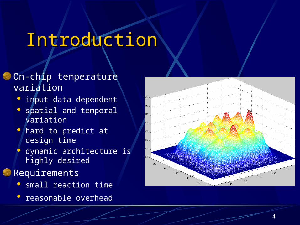
On-chip temperature variation input data dependent spatial and temporal variation hard to predict at design time dynamic architecture is highly

desired

Requirements small reaction time reasonable overhead

5

IntroductionIntroduction

On-chip temperature variation input data dependent spatial and temporal variation hard to predict at design time dynamic architecture is highly

desired

Requirements small reaction time reasonable overhead

6

IntroductionIntroduction

On-chip temperature variation input data dependent spatial and temporal variation hard to predict at design time dynamic architecture is highly

desired

Requirements small reaction time reasonable overhead

7

IntroductionIntroduction

On-chip temperature variation input data dependent spatial and temporal variation hard to predict at design time dynamic architecture is highly

desired

Requirements small reaction time reasonable overhead

8

MotivationMotivation

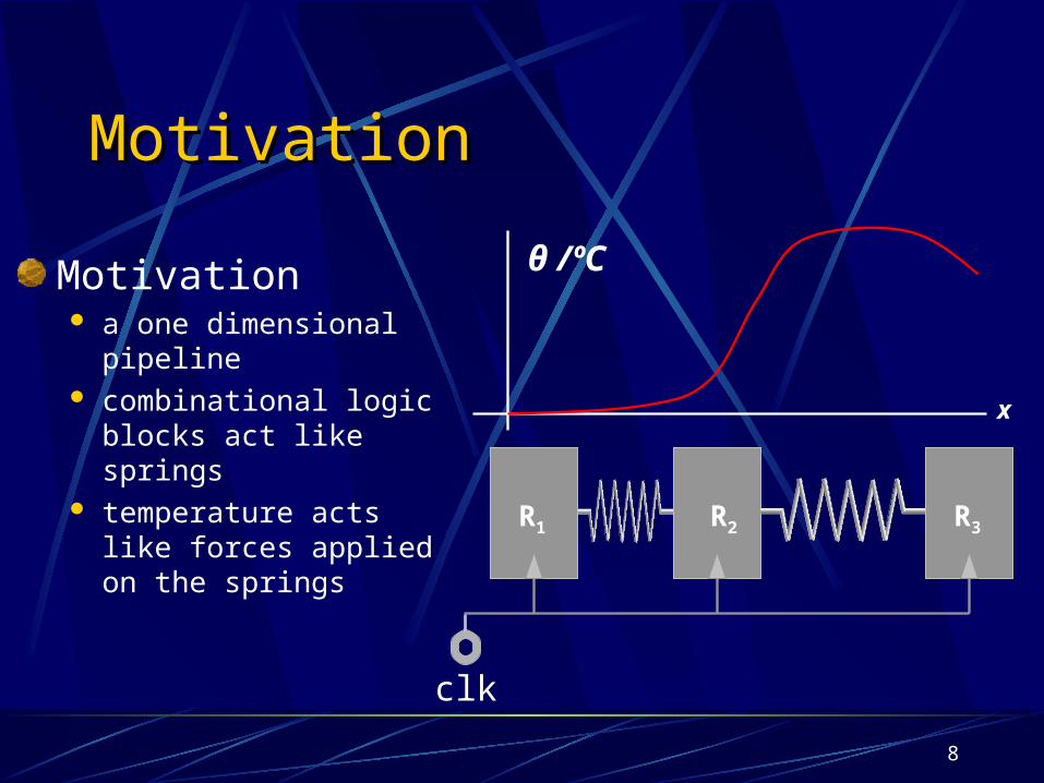
Motivation a one dimensional

pipeline combinational logic blocks

act like springs temperature acts like

forces applied on the springs

R1 R2 R3

θ /ºC

x

clk

9

x

MotivationMotivation

Motivation a one dimensional

pipeline combinational logic blocks

act like springs temperature acts like

forces applied on the springs

what if the clock skews act like springs also?

R1 R2 R3

clk

θ /ºC

10

MotivationMotivationClock skews xi : clock signal arrival time at register Ri

Di,i+1 = Tc-q+Tlogic(max)+Tint+Tsetup

di,i+1 = Tc-q+Tlogic(min)+Tint+Thold

Clock Skew Constraints – di,i+1 ≤ xi – xi+1 ≤ Tcp – Di,i+1

R1 R2 R3

clk

setup time constraint

hold time constraint

11

MotivationMotivationClock skew constraints – di,i+1 ≤ xi – xi+1 ≤ Tcp – Di,i+1

Observation di,i+1, –(xi – xi+1) and Di,i+1 should be made to have the

same dependency on temperature

R1 R2 R3

clk

12

MotivationMotivation

How does di,i+1 and Di,i+1 depend on temperature? HSPICE simulation v.s.

linear model we only need to make the

clock skews linearly dependant on temperature

40 60 80 100 1201

1.02

1.04

1.06

1.08

1.1

1.12

1.14

1.16

Temperature (ºC)N

orm

. Del

ay

HSPICELinear model

13

MotivationMotivation

Constraints revisited assuming the operating temperature

ranging between θmin and θmax

the constraints form a quadrangle we only need to couple xi – xi ＋ 1 with

the local temperature θi,i+1, and make it a line lying strictly within the

the quadrangle

θmax

td

Tcp – Di,i+1(θi,i+1)

– di,i+1(θi,i+1)

(xi – xi ＋ 1)(θi,i+1)θmin

– di,i+1 ≤ xi – xi+1 ≤ Tcp – Di,i+1

θ

14

SACTA: ArchitectureArchitecture

Self-Adjusting Clock Tree Architecture xi – xi+1 = (fi – fi+1– si) + ki (Δθ), where Δθ = θmax – θ Automatic Temperature Adjustable (ATA) skew buffer Temperature-insensitive (fixed) skew buffer

f1 fi fi+1 fn

Ri Ri+1 RnR1

s1-k1 Δθ si-ki Δθ si+1-ki+1 Δθclk

15

SACTASACTA: Skew BufferBuffer Design

Fixed skew buffer bias the gates to Zero Temperature

Coefficient point VZTC

Vdd

Vdd

M1

M2

M3 M4

IZTC

IZTC

VZTC

+

–

VZTCRef

min-size min-size

VZTC

Fixed Skew Buffer

Wmin, [Lmin, 5Lmin]

16

ATA skew buffer

SACTA: Skew Buffer Design

Fixed Buffers

VddVZTC Ref

min-size min-size

Wmin, [Lmin, 5Lmin]

17

SACTASACTA: OptimizationOptimization

Optimizing the clock tree fi and si positively related to the

overhead minimizing the sum of fi and si

Constraints skew buffer design constraints:

si ≥ smin, fi ≥ fmin, ki – λsi = 0

timing correctness: for θ = θmax, θmin,

–di,i+1(θ)≤(xi–xi+1)(θ)≤Tcp – Di,i+1(θ)

td

Tcp – Di,i+1(θi,i+1)

– di,i+1(θi,i+1)

(xi – xi ＋ 1)(θ i,i+1)θmin θmax

18

SACTA optimization formulation

SACTASACTA: OptimizationOptimization

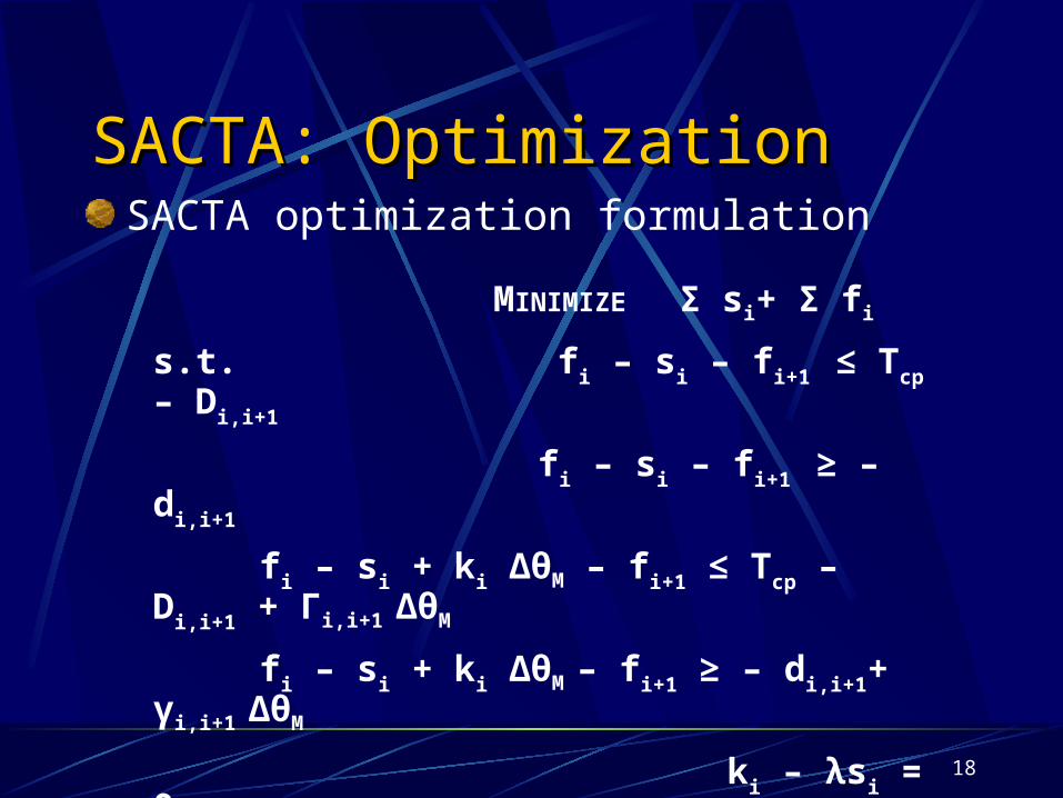
MINIMIZE Σ si+ Σ fi

s.t. fi – si – fi+1 ≤ Tcp – Di,i+1

fi – si – fi+1 ≥ – di,i+1

fi – si + ki ΔθM – fi+1 ≤ Tcp – Di,i+1 + Γi,i+1 ΔθM

fi – si + ki ΔθM – fi+1 ≥ – di,i+1+ γi,i+1 ΔθM

ki – λsi = 0

si ≥ smin, fi, fi+1 ≥ fmin

i = 1, 2, …, n-1

19

Transforming the problem into a network flow formulation defining four new variables fi

Δ = fi – fmin

siΔ

= si – smin ui = fi – si – fi+1+ di,i+1

vi = fi – si(1-λΔθM) – fi+1 + di,i+1 – γi,i+1 ΔθM the optimization problem can be rewritten as

SACTA: OptimizationOptimization

20

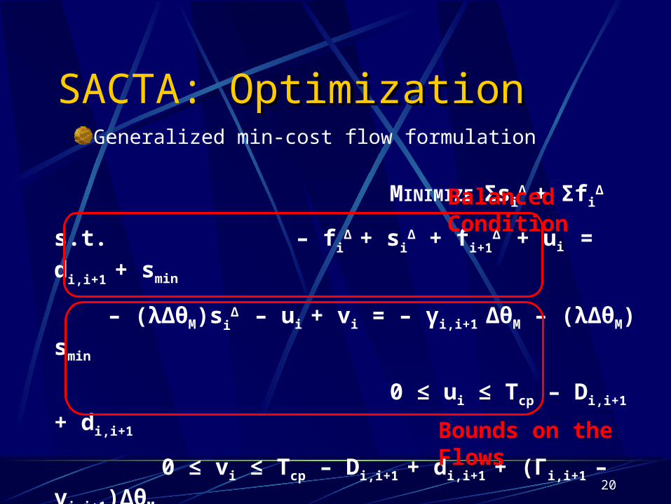
SACTA: OptimizationOptimization

MINIMIZE ΣsiΔ

+ ΣfiΔ

s.t. – fiΔ

+ siΔ + fi+1

Δ + ui = di,i+1 + smin

– (λΔθM)siΔ – ui + vi = – γi,i+1 ΔθM – (λΔθM) smin

0 ≤ ui ≤ Tcp – Di,i+1 + di,i+1

0 ≤ vi ≤ Tcp – Di,i+1 + di,i+1 + (Γi,i+1 – γi,i+1)ΔθM

siΔ, fi

Δ , fi+1

Δ ≥ 0

i = 1, 2, …, n-1

Generalized min-cost flow formulation

Balanced Condition

Bounds on the Flows

21

SACTA: OptimizationOptimization

Balance Condition:

– fiΔ

+ siΔ + fi+1

Δ + ui = di,i+1 + smin

– (λΔθM)siΔ – ui + vi = – γi,i+1 ΔθM – (λΔθM) smin

Graph based depiction of the constraints

0, Tcp – Di,i+1+ di,i+1 , ui

1, +∞, fiΔ 1, +∞, fi+1

Δ

pi

qi

cost, capacity, flowp q

1, +∞, siΔ

0, Tcp– Di,i+1+di,i+1+(Γi,i+1 – γi,i+1 ) ΔθM, vi

Bounds on the Flows:

0 ≤ vi ≤ Tcp – Di,i+1 + di,i+1 + (Γi,i+1 – γi,i+1)ΔθM

0 ≤ ui ≤ Tcp – Di,i+1 + di,i+1

siΔ, fi

Δ , fi+1

Δ ≥ 0

22

SACTA: OptimizationOptimizationGraph based depiction of the constraints

0, Tcp – Di,i+1+ di,i+1 , ui

cost, capacity, flow

1, +∞, fiΔ 1, +∞, fi+1

Δ

pi

qi

p q

1, +∞, si

0, Tcp– Di,i+1+di,i+1+(Γi,i+1 – γi,i+1 ) ΔθM, vi

pn-1

qn-1

p1 p2 p3

q1 q2 q3

w

23

Experimental ResultsExperimental Results

Experiments six different systolic

pipelines both balanced and

unbalanced pipelines are examined

targeting range θmax = 125 ºC, θmin = 25 ºC

VHDL Description

Technology Lib

Di,i+1 and di,i+1

Scale to 90 nm

Γi,i+1 and γi,i+1

Clk Tree Optimization

SACTA Specifications

Delay-θ Model

Tcp, θmax, θmin

SynopsysDC

VHDL Description

Technology Lib

Di,i+1 and di,i+1

Scale to 90 nm

Γi,i+1 and γi,i+1

Clk Tree Optimization

SACTA Specifications

Delay-θ Model

Tcp, θmax, θmin

SynopsysDC

24

Experimental ResultsExperimental ResultsExperimental results uniform temperature distribution maximum permissible temperature

50

60

70

80

90

100

110

120

130

P B P U RB RU FB FU

Max Temperature w/ SACTA Max Temperature w/o SACTA

50

60

70

80

90

100

110

120

130

P B P U RB RU FB FU

Max Temperature w/ SACTAMax Temperature w/ SACTA Max Temperature w/o SACTAMax Temperature w/o SACTA

six different pipelines

T/°C

25

Experimental ResultsExperimental ResultsExperimental results uniform temperature distribution (125 ºC) relative performance improvement

six different pipelines

RP

0.85

0.9

0.95

1

1.05

1.1

1.15

P B P U RB RU FB FU

Normalized Max Freq w/ SACTA Normalized Max Freq w/o SACTA

0.85

0.9

0.95

1

1.05

1.1

1.15

P B P U RB RU FB FU

Normalized Max Freq w/ SACTANormalized Max Freq w/ SACTA Normalized Max Freq w/o SACTANormalized Max Freq w/o SACTA

26

Experimental ResultsExperimental ResultsExperimental results various temperature profiles X: timing error, Y: no timing error

Thermal Profile/ºC Pipelines w/o SACTA Pipelines w/ SACTA

s1 s2 s3 s4 s5 PB PU RB RU FB FU PB PU RB RU FB FU

125 115 110 107 105 X X X X X X Y Y Y Y Y Y

105 107 110 115 125 X X Y Y X X Y Y Y Y Y Y

100 105 110 105 100 X X Y Y X X Y Y Y Y Y Y

135 125 120 117 115 X X X X X X X Y X Y X Y

115 117 120 125 135 X X X X X X X Y X X X X

27

Experimental ResultsExperimental Results

Experimental results hardware overhead

PB PU RB RU FB FU

On-Tree Inv Num 67 51 67 50 67 53

Pipeline Cell Num 2082 2082 1572 1572 498 498

28

ConclusionsConclusions

Temperature variation affects circuit timing

Dynamic architectures are required

SACTA architecture, skew buffer design, optimization SACTA enhances system robustness and performance hardware overhead of SACTA is small

29