1

Jorge Nocedal Northwestern University

With S. Hansen, R. Byrd and Y. Singer

IPAM, UCLA, Feb 2014

A Stochastic Quasi-Newton Method for Large-Scale Learning

Propose a robust quasi-Newton method that operates in the stochastic approximation regime

• purely stochastic method (not batch) – to compete with stochatic gradient (SG) method

• Full non-diagonal Hessian approximation• Scalable to millions of parameters

2

Goal

wk+1 =wk −αkHk∇F(wk)

3

Outline

Are iterations of this following form viable? - theoretical considerations; iteration costs - differencing noisy gradients?

Key ideas: compute curvature information pointwise at regular intervals, build on strength of BFGS updating recalling that it is an overwriting (and not averaging process)

- results on text and speech problems - examine both training and testing errors

wk+1 =wk −αkHk∇f(wk)

4

Problem

minw∈° n F(w)=E[ f(w;ξ)]

Stochastic function of variable w with random variable ξApplications• Simulation optimization• Machine learning ξ = selection of input-output pair (x, z)

  f (w,ξ) = f(w,xi ,zi ) =l (h(w;xi ),zi )

F(w)=1N

f (w;xi ,zi )i=1

N

∑

Algorithm not (yet) applicable to simulation based optimization

For loss function

Robbins-Monro or stochastic gradient method

using stochastic gradient (estimator)

min-batch

5

Stochastic gradient method

wk+1 =wk −αk∇F(wk) α k = O(1 / k)

 ∇F(wk) :        E [∇F(w)]=∇F(w) 

∇F(wk) =1b

∇i∈S∑ f(w;xi ,zi ),      |S |=b

F(w)=1N

f (w;xi ,zi )i=1

N

∑

b=|S|<< N

1. Is there any reason to think that including a Hessian approximation will improve upon stochastic gradient method?

2. Iteration costs are so high that even if method is faster than SG in terms of training costs it will be a weaker learner

6

Why it won’t work ….

wk+1 =wk −αkHk∇F(wk)

wk+1 =wk −αkBk−1∇F(wk), αk =O(1 / k)

Number of iterations needed to compute an epsilon-accurate solution:

Bk =∇2F(w* )Bk =I

Depends on the Hessian at true solution and the gradient covariance matrix

Depends on the condition number of the Hessian at the true solution

Completely removes the

dependency on the condition number

(Murata 98); cf Bottou-Bousquet

7

Theoretical Considerations

Motivation for choosing Bk → ∇2F        Quasi-Newton

Assuming we obtain efficiencies of classical quasi-Newtonmethods in limited memory form

• Each iteration requires 4Md operations• M = memory in limited memory implementation; M=5• d = dimension of the optimization problem

8

Computational cost

wk+1 =wk −αkHk∇f(wk)

4Md +d= 21d    vs     d      Stochastic gradient

method

cost of computing

       ∇f(wk)

• assuming a min-batch b=50• cost of stochastic gradient = 50d

Use of small mini-batches will be a game-changer b =10, 50, 100

9

Mini-batching

4Md +bd=20d+ 50d    vs     50d     

∇F(wk) =1b

∇i∈S∑ f(w;xi ,zi ),      |S | =b

70d vs 50d

Mini-batching makes operation counts favorable but does not resolve challenges related to noise

1. Avoid differencing noise• Curvature estimates cannot suffer from sporadic spikes in noise

(Schraudolph et al. (99), Ribeiro et at (2013)• Quasi-Newton updating is an overwriting process not an averaging

process• Control quality of curvature information

2. Cost of curvature computation

Use of small mini-batches will be a game-changer b =10,50,100

10

Game changer? Not quite…

11

Desing of Stochastic Quasi-Newton Method

wk+1 =wk −αkHk∇f(wk)

Propose a method based on the famous BFGS formula• all components seem to fit together well• numerical performance appears to be strong

Propose a new quasi-Newton updating formula• Specifically designed to deal with noisy gradients• Work in progress

12

Review of the deterministic BFGS method

wk+1 =wk −αkBk−1∇F(wk)

At every iteration compute and save

     yk =∇F(wk+1 )−∇F(wk), sk =wk+1 −wk,

wk+1 =wk −αkHk∇F(wk)

H k+1 =(I −ρkskykT )Hk(I −ρkyksk

T )+ ρkskskT ρk =

1

skT yk

Correction pairs yk , sk uniquely determine BFGS updating

13

The remarkable properties of BFGS method (convex case)

tr(Bk+1) =tr(Bk)−° Bksk°´skTBksk

+° yk°´2

ykTsk

detBk+1 = detBk

ykTskskTsk

skTsk

skTBksk

° (Bk −∇F(x* ))sk°´°´sk°´

→ 0

If the algorithm takes a bad step, matrix is corrected...

Superlinear convergence; global convergence

for strongly convex problems, self-correction properties

Only need to approximate Hessian in a subspace

Powell 76

Byrd-N 89

14

Adaptation to stochastic setting

Cannot mimic classical approach and update after each iteration

Since batch size b is small this will yield highly noisy curvature estimates

yk =∇F(wk+1 )−∇F(wk), sk =wk+1 −wk

Instead: Use a collection of iterates to define the correction

pairs

15

Stochastic BFGS: Approach 1

Define two collections of size L:

wi ,∇F(wi ) |i ∈I{ } , wj ,∇F(wj ) | j ∈J{ }    |I |=|J |=L

wI =1|I |

wii∈I∑ , gI =

1|I |

∇i∈I∑ F(wi )

s =wI −wj , y= gI −gJ

Define average iterate/gradient:

New curvature pair:

wk+1 =wk −αk∇F(wk)wk+1 =wk −αkHt∇F(wk)

wi ,∇F(wi ) |i ∈I{ }

w j ,∇F(wj ) | j ∈J{ }

wi ,∇F(wi ) |i ∈I{ }

w j ,∇F(wj ) | j ∈J{ }

wi ,∇F(wi ) |i ∈I{ }

s =wI −wJ

y=gI −gJ

       →  H2

s =wI −wJ

y=gI −gJ

→  H1

s =wI −wJ

y=gI −gJ

        →  H3

16

Stochastic L-BFGS: First Approach

17

Stochastic BFGS: Approach 1

We could not make this work in a robust manner!

1. Two sources of error• Sample variance• Lack of sample uniformity

2. Initial reaction• Control quality of average gradients• Use of sample variance … dynamic sampling

s =wI −wJ ,y= gI −gJ

Proposed Solution Control quality of curvature y estimate directly

Standard definition

arises from

Hessian-vector products are often available

Define curvature vector for L-BFGS via a Hessian-vector product perform only every L iterations

y  ←  ∇2F(wI )s

y =∇F(wI )−∇F(wJ )

18

∇F(wI )−∇F(wJ ) ≈∇2F(wI )(wI −wJ )

Key idea: avoid differencing

y =∇2F(wI )s

∇2F(wk)s=1bH

∇i∈SH

∑ 2f (w;xi ,zi )s,         |SH | =bH

19

Structure of Hessian-vector product

Mini-batch stochastic gradient

1. Code Hessian-vector product directly2. Achieve sample uniformity automatically (c.f. Schraudolph)

3. Avoid numerical problems when ||s|| is small

4. Control cost of y computation

wk+1 =wk −αk∇F(wk)wk+1 =wk −αkHt∇F(wk)

wi | i ∈I{ }

w j | j ∈J{ }

wi | i ∈I{ }

w j | j ∈J{ }

wi | i ∈I{ }

s =wI −wJ

y=∇2F(wI )s→  H2

s =wI −wJ

y=∇2F(wI )s      →  H1

s =wI −wJ

y=∇2F(wI )s          →  H3

20

The Proposed Algorithm

• b: stochastic gradient batch size

• bH: Hessian-vector batch size

• L: controls frequency of quasi-Newton updating

• M: memory parameter in L-BFGS updating M=5

- use limited memory form

21

Algorithmic Parameters

22

Need Hessian to implement a quasi-Newton method?

Are you out of your

mind?

We don’t need Hessian-vector product, but it has many

Advantages: complete freedom in sampling and accuracy

ŦŒ ä śϖ⌥ ħ??

23

Numerical Tests

wk+1 =wk −αkHk∇f(wk)      αk =β / k

wk+1 =wk −αk∇f(wk)      αk =β / k     Stochastic gradient

method (SGD)

Stochastic quasi-Newton

method (SQN)

parameter β to be fixed at start for each method;found by bisection procedure

It is well know that SGD is highly sensitive to choice of steplength,

and so will be the SQN method (though perhaps less)

• b = 50, 300, 1000

• M = 5, L = 20 bH = 100024

RCV1 Problem n = 112919, N = 688329

Accessed

data points;

includes Hessian-

vector products

sgd

sqn

• b = 100, 500 , M = 5, L = 20, bH = 1000

25

Speech Problem n= 30315, N = 191607

sgd

sqn

26

Varying Hessian batch bH: RCV1

b=300

27

Varying memory size M in limited memory BFGS: RCV1

28

Varying L-BFGS Memory Size: Synthetic problem

29

Generalization Error: RCV1 Problem

SGD

SQN

• Synthetically Generated Logistic Regression: Singer et al

– n = 50, N = 7000

– Training data:.

• RCV1 dataset

– n = 112919, N = 688329

– Training data: xi ∈[0,1]n, zi ∈[0,1]

xi ∈° n, zi ∈[0,1]

• SPEECH dataset

– NF = 235, |C| = 129

– n = NF x |C| --> n= 30315, N = 191607

– Training data: xi ∈° NF , zi ∈[1,129]30

Test Problems

Iteration Costs

• mini-batch stochastic gradient

SQNSGD

• mini-batch stochastic gradient

• Hessian-vector product every L iterations

• matrix-vector product

31

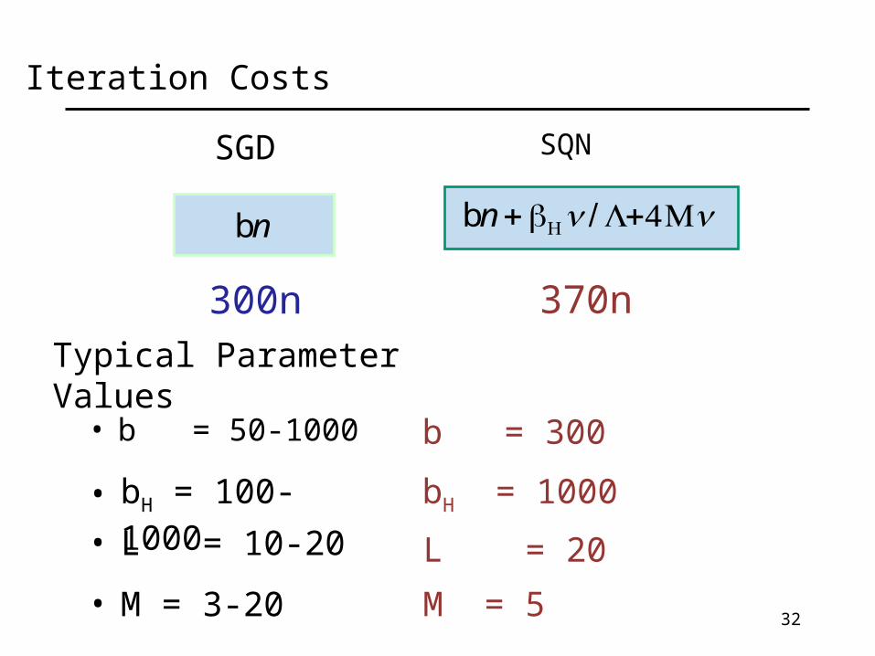
• b = 50-1000

bn bn +bHn/ L+4Mn

SGD SQN

• bH = 100-1000

• L = 10-20

• M = 3-20

Typical Parameter Values

b = 300

bH = 1000

L = 20

M = 5

300n 370n

32

Iteration Costs

33

Hasn’t this been done before?

Hessian-free Newton method: Martens (2010), Byrd et al (2011)

- claim: stochastic Newton not competitive with stochastic BFGS Prior work: Schraudolph et al. - similar, cannot ensure quality of y - change BFGS formula in one-sided form

34

Supporting theory?

Work in progress: Figen Oztoprak, Byrd, Soltnsev

- combine classical analysis Murata, Nemirovsky et a - and asumptotic quasi-Newton theory - effect on constants (condition number) - invoke self-correction properties of BFGS

Practical Implementation: limited memory BFGS - loses superlinear convergence property - enjoys self-correction mechanisms

SGD:

SQN:

b adp/iter

b + bH/L adp/iter

bn + bHn/L +4Mn work/iter

bn work/iter

bH=1000, M=5, L=200

Parameters L, M and bH provide freedom in adapting the SQN method to a specific application 35

Small batches: RCV1 Problem

36

Alternative quasi-Newton framework

BFGS method was not derived with noisy gradients in mind

- how do we know it is an appropriate framework -

Start from scratch - derive quasi-Newton updating formulas tolerant to noise

Define quadratic model around a reference point z

Using a collection indexed by I , natural to require

i.e. residuals are zero in expectation

Not enough information to determine the whole model

37

Foundations

qz (w)= f(w) + gT (w−z) +12(w−z)T B(w−z)

[∇qj∈I∑ (wj )−∇f(wj )] =0

Given a collection I, choose model q to minimize

Differentiating w.r.t. g:

Encouraging: obtained residual condition

38

Mean square error

F(g, B)=  °´j∈I∑  ∇q(wj )−∇f(wj )°´2=0

ming,B °´j∈I∑ Bsk + g−∇f (wj )°´

2

Define sk =wk −z,  restate problem as

j∈I∑ {Bsk + g−∇f (wj )} =0

qz (w)=gT (w−z) +12(w−z)T B(w−z)

39

The End