1 ka-fu wong university of hong kong modeling cycles: ma, ar and arma models
Post on 19-Dec-2015
215 views
TRANSCRIPT

1
Ka-fu WongUniversity of Hong Kong
Modeling Cycles: MA, AR and ARMA Models
2
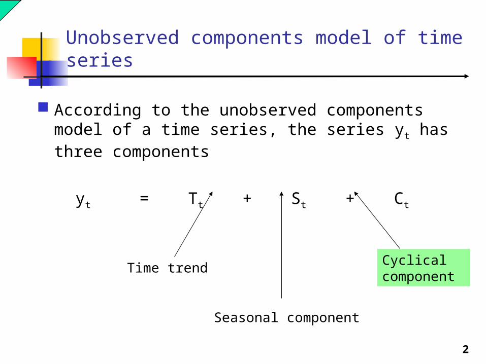
Unobserved components model of time series
According to the unobserved components model of a time series, the series yt has three components
yt = Tt + St + Ct
Time trend
Seasonal component
Cyclical component

3
The Starting Point
Let yt denote the cyclical component of the time series.
We will assume, unless noted otherwise, that yt is a zero-mean covariance stationary process. Recall that part of this assumption is that the time
series originated infinitely far back into the past and will continue infinitely far into the future, with the same mean, variance, and autocovariance structure.
The starting point for introducing the various kinds of econometric models that are available to describe stationary processes is the Wold Representation Theorem (or, simply, Wold’s theorem).
4
Wold’s theorem
According to Wold’s theorem, if yt is a zero mean covariance stationary process than it can be written in the form:
...221100
ttt
iitit bbbby
where the ε’s are (i) WN(0,σ2), (ii) b0 = 1, and (iii)
0
2
iib
In other words, each yt can be expressed in terms of a single linear function of current and (possibly an infinite number of) past drawings of the white noise process, εt.
If yt depends on an infinite number of past ε’s, the weights on these ε’s, i.e., the bi’s must be going to zero as i gets large (and they must be going to zero at a fast enough rate for the sum of squared bi’s to converge).
5
Innovations
εt is called the innovation in yt because εt is that part of yt not predictable from the past history of yt, i.e., E(εt │yt-1,yt-2,…)=0
Hence, the forecast (conditional expectation) E(yt │yt-1,yt-2,…)
= E(yt │εt-1,εt-2,…)
= E(εt + b1εt-1 + b2εt-2 +…│εt-1,εt-2,…)
= E(εt │εt-1,εt-2,…) + E(b1εt-1 + b2εt-2 +…│εt-1,εt-2,…)
= 0 + (b1εt-1 + b2εt-2 +…)
= b1εt-1 + b2εt-2 +…And, the one-step ahead forecast error yt - E(yt │yt-1,yt-2,…)
= (εt + b1εt-1 + b2εt-2 +…)-(b1εt-1 + b2εt-2 +…)
= εt

6
Mapping Wold to a variety of models
The one-step-ahead forecast error isyt - E(yt │yt-1,yt-2,…) = (εt + b1εt-1 + b2εt-2 +…)-(b1εt-1 + b2εt-2 +…)= εt
Thus, according to the Wold theorem, each yt can be expressed as the same weighted average of current and past innovations (or, 1-step ahead forecast errors).
It turns out that the Wold representation can usually be well-approximated by a variety of models that can expressed in terms of a very small number of parameters. the moving-average (MA) models, the autoregressive (AR) models, and the autoregressive moving-average (ARMA) models.

7
Mapping Wold to a variety of models
For example, suppose that the Wold representation has the form:
0iit
it by
for some b, 0 < b < 1. (i.e., bi = bi)
Then it can be shown that
yt = byt-1 + εt
which is an AR(1) model.
8
Mapping Wold to a variety of models
The procedure we will follow is to describe each of these three types of models and, especially, the shapes of the autocorrelation and partial autocorrelations that they imply.
Then, the game will be to use the sample autocorrelation/partial autocorrelation functions of the data to “guess” which kind of model generated the data. We estimate that model and see if it provide a good fit to the data. If yes, we proceed to the forecasting step using this estimated model of the cyclical component. If not, we guess again …
9
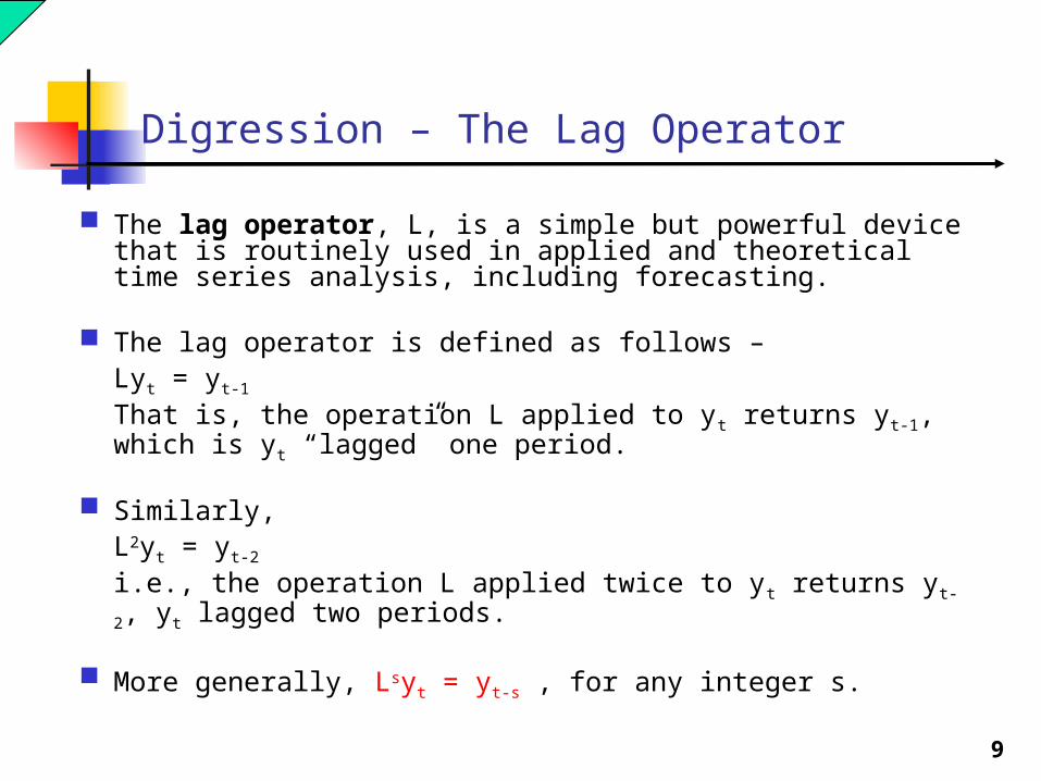
Digression – The Lag Operator
The lag operator, L, is a simple but powerful device that is routinely used in applied and theoretical time series analysis, including forecasting.
The lag operator is defined as follows –Lyt = yt-1
That is, the operation L applied to yt returns yt-1, which is yt “lagged” one period.
Similarly,L2yt = yt-2
i.e., the operation L applied twice to yt returns yt-2, yt lagged two periods.
More generally, Lsyt = yt-s , for any integer s.
10
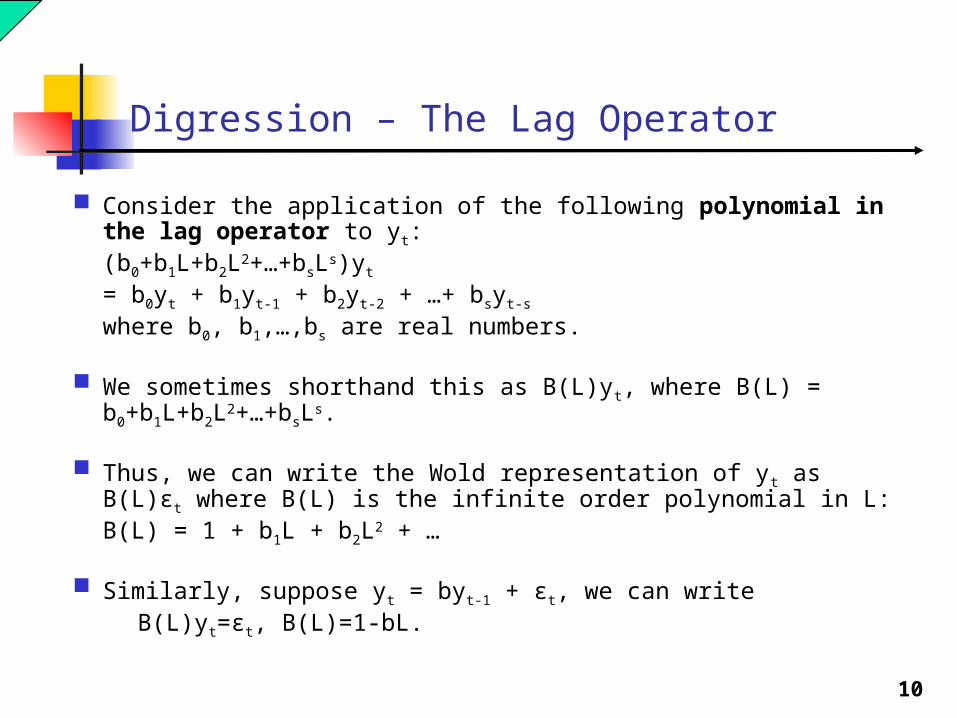
Digression – The Lag Operator
Consider the application of the following polynomial in the lag operator to yt:
(b0+b1L+b2L2+…+bsLs)yt
= b0yt + b1yt-1 + b2yt-2 + …+ bsyt-s
where b0, b1,…,bs are real numbers.
We sometimes shorthand this as B(L)yt, where B(L) = b0+b1L+b2L2+…+bsLs.
Thus, we can write the Wold representation of yt as B(L)εt where B(L) is the infinite order polynomial in L:
B(L) = 1 + b1L + b2L2 + …
Similarly, suppose yt = byt-1 + εt, we can write B(L)yt=εt, B(L)=1-bL.
11
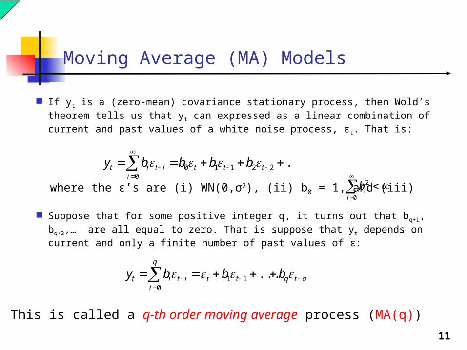
Moving Average (MA) Models
If yt is a (zero-mean) covariance stationary process, then Wold’s theorem tells us that yt can expressed as a linear combination of current and past values of a white noise process, εt. That is:
...221100
ttt
iitit bbbby
where the ε’s are (i) WN(0,σ2), (ii) b0 = 1, and (iii)
0
2
iib
Suppose that for some positive integer q, it turns out that bq+1, bq+2,… are all equal to zero. That is suppose that yt depends on current and only a finite number of past values of ε:
qtqtt
q
iitit bbby
...11
0
This is called a q-th order moving average process (MA(q))

12
Realization of two MA(1) processesyt = εt + θεt-1
13
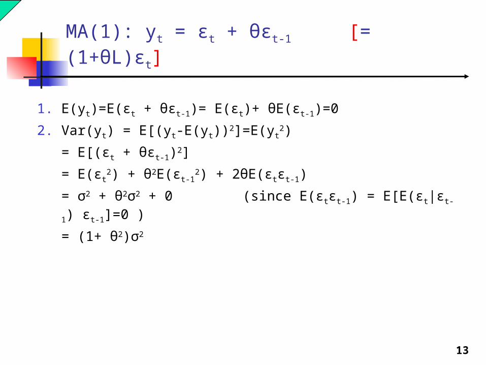
MA(1): yt = εt + θεt-1 [= (1+θL)εt]
1. E(yt)=E(εt + θεt-1)= E(εt)+ θE(εt-1)=0
2. Var(yt) = E[(yt-E(yt))2]=E(yt2)
= E[(εt + θεt-1)2]
= E(εt2) + θ2E(εt-1
2) + 2θE(εtεt-1)
= σ2 + θ2σ2 + 0 (since E(εtεt-1) = E[E(εt|εt-1) εt-
1]=0 )
= (1+ θ2)σ2
14
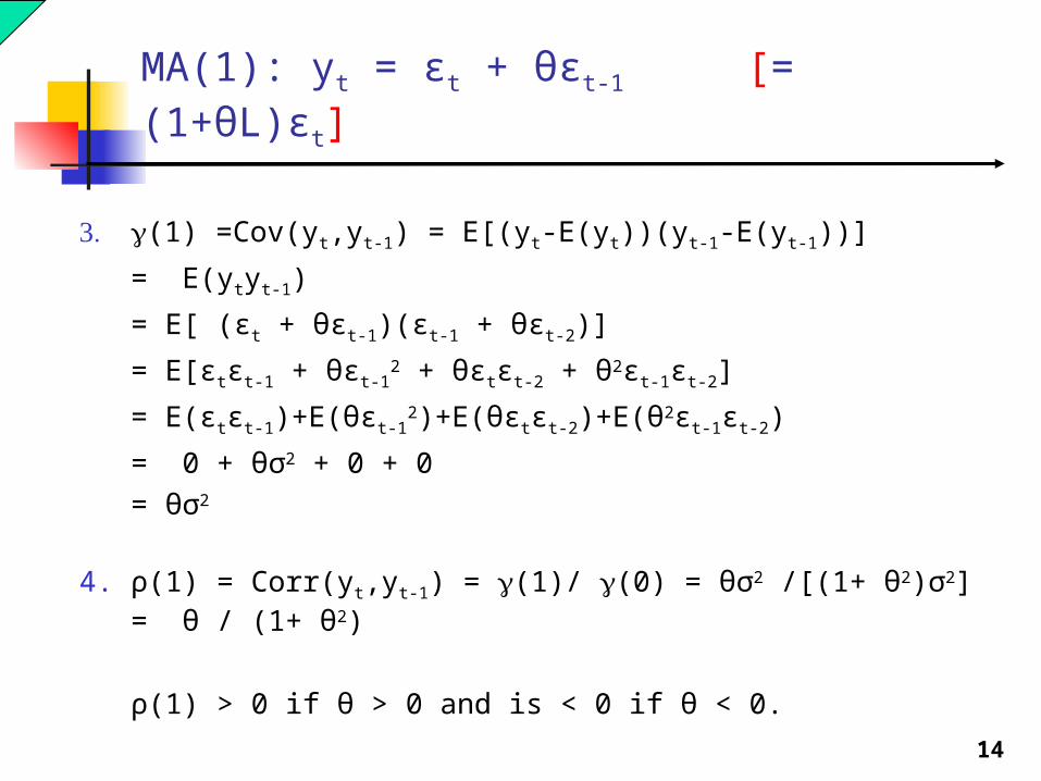
MA(1): yt = εt + θεt-1 [= (1+θL)εt]
3. (1) =Cov(yt,yt-1) = E[(yt-E(yt))(yt-1-E(yt-1))]
= E(ytyt-1)
= E[ (εt + θεt-1)(εt-1 + θεt-2)]
= E[εtεt-1 + θεt-12 + θεtεt-2 + θ2εt-1εt-2]
= E(εtεt-1)+E(θεt-12)+E(θεtεt-2)+E(θ2εt-1εt-2)
= 0 + θσ2 + 0 + 0 = θσ2
4. ρ(1) = Corr(yt,yt-1) = (1)/ (0) = θσ2 /[(1+ θ2)σ2] = θ / (1+ θ2)
ρ(1) > 0 if θ > 0 and is < 0 if θ < 0.
15
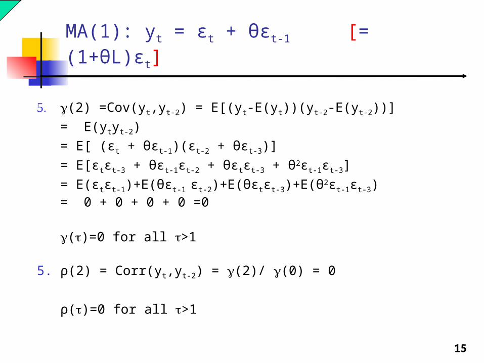
MA(1): yt = εt + θεt-1 [= (1+θL)εt]
5. (2) =Cov(yt,yt-2) = E[(yt-E(yt))(yt-2-E(yt-2))]
= E(ytyt-2)
= E[ (εt + θεt-1)(εt-2 + θεt-3)]
= E[εtεt-3 + θεt-1εt-2 + θεtεt-3 + θ2εt-1εt-3]
= E(εtεt-1)+E(θεt-1 εt-2)+E(θεtεt-3)+E(θ2εt-1εt-3)= 0 + 0 + 0 + 0 =0
()=0 for all >1
5. ρ(2) = Corr(yt,yt-2) = (2)/ (0) = 0
ρ()=0 for all >1
16
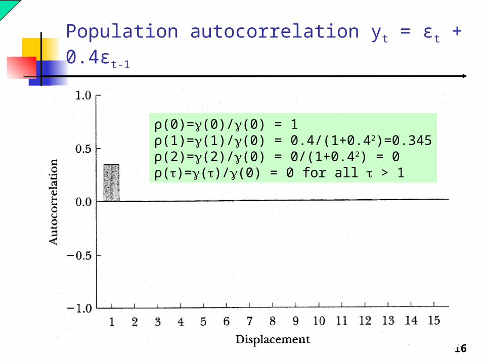
Population autocorrelation yt = εt + 0.4εt-1
ρ(0)=(0)/(0) = 1ρ(1)=(1)/(0) = 0.4/(1+0.42)=0.345ρ(2)=(2)/(0) = 0/(1+0.42) = 0ρ()=()/(0) = 0 for all > 1
17
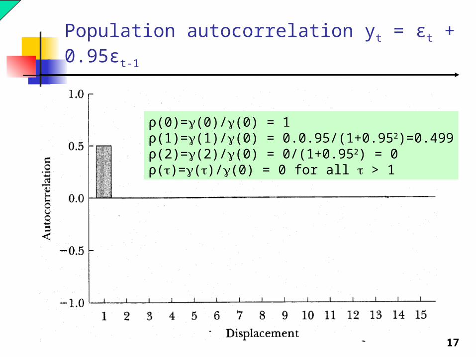
Population autocorrelation yt = εt + 0.95εt-
1
ρ(0)=(0)/(0) = 1ρ(1)=(1)/(0) = 0.0.95/(1+0.952)=0.499ρ(2)=(2)/(0) = 0/(1+0.952) = 0ρ()=()/(0) = 0 for all > 1
18
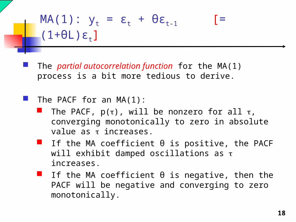
MA(1): yt = εt + θεt-1 [= (1+θL)εt]
The partial autocorrelation function for the MA(1) process is a bit more tedious to derive.
The PACF for an MA(1): The PACF, p(), will be nonzero for all , converging
monotonically to zero in absolute value as increases. If the MA coefficient θ is positive, the PACF will exhibit
damped oscillations as increases. If the MA coefficient θ is negative, then the PACF will
be negative and converging to zero monotonically.

19
Population Partial Autocorrelation yt = εt + 0.4εt-1
20
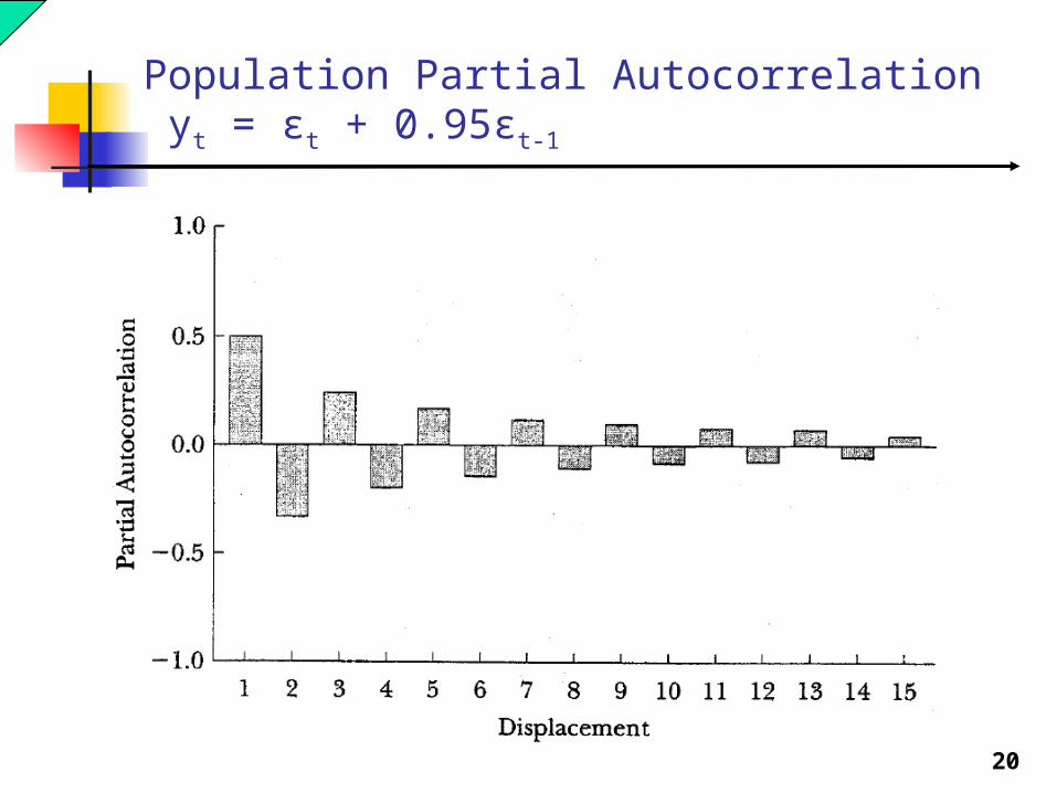
Population Partial Autocorrelation yt = εt + 0.95εt-1

21
Forecasting yT+h E(yT+h│yT,yT-1,…)
E(yT+h│yT,yT-1,…) = E(yT+h│εT,εT-1,…)since each yt can be expressed as a function of εT,εT-1,
… E(yT+1│εT,εT-1,…) = E(εT+1+ θεT│εT,εT-1,…)
since yT+1 = εT+1+ θεT
= E(εT+1│εT,εT-1,…) + E(θεT│εT,εT-1,…)= θεT
E(yT+2│εT,εT-1,…)=E(εT+2+ θεT+1│εT,εT-1,…)= E(εT+2│εT,εT-1,…)+E(θεT+1│εT,εT-1,…)= 0…
E(yT+h│yT,yT-1,…) = E(yT+h│εT,εT-1,…)= θεT for h = 1= 0 for h > 1
22
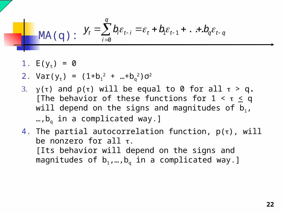
MA(q):
1. E(yt) = 0
2. Var(yt) = (1+b12 + …+bq
2)σ2
3. () and ρ() will be equal to 0 for all > q. [The behavior of these functions for 1 < < q will depend on the signs and magnitudes of b1,…,bq in a complicated way.]
4. The partial autocorrelation function, p(), will be nonzero for all . [Its behavior will depend on the signs and magnitudes of b1,…,bq in a complicated way.]
qtqtt
q
iitit bbby
...11
0

23
MA(q):
5. E(yT+h│yT,yT-1,…) = E(yT+h│εT, εT-1,…) = ?
yT+1 = εT+1 + θ1εT + θ2εT-1 + … + θqεT-q+1
So, E(yT+1│ εT, εT-1,…) = θ1εT +θ2εT-1+…+ θqεT-q+1
More generally,E(yT+h│εT, εT-1,…) = θhεT + … + θqεT-q+h for h < q
0 for h > q
qtqtt
q
iitit bbby
...11
0

24
Autoregressive Models (AR(p))
In certain circumstances, the Wold form for yt,
...22110
ttt
iitit bbby
can be “inverted” into a finite-order autoregressive form, i.e.,
yt = φ1yt-1+ φ2yt-2+…+ φpyt-p+εt
This is called a p-th order autoregressive process AR(p)).
Note that it has p unknown coefficients: φ1,…, φp
Note too that the AR(p) model looks like a standard linear regression model with zero-mean, homoskedastic, and serially uncorrelated errors.

25
AR(1): yt = φyt-1 + εt
26
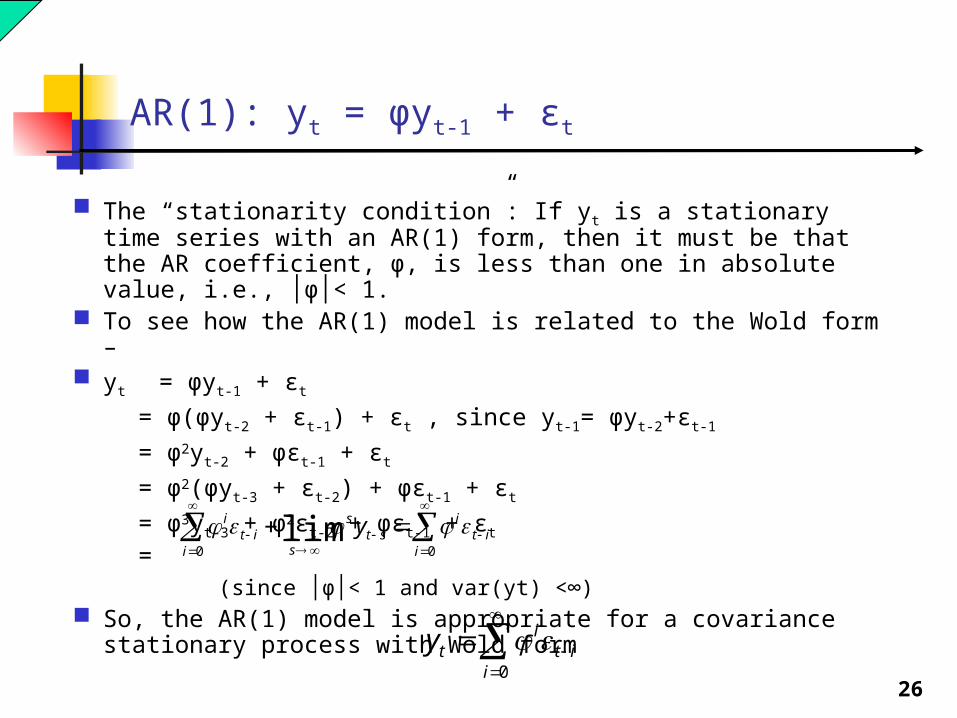
AR(1): yt = φyt-1 + εt
The “stationarity condition”: If yt is a stationary time series with an AR(1) form, then it must be that the AR coefficient, φ, is less than one in absolute value, i.e., │φ│< 1.
To see how the AR(1) model is related to the Wold form – yt = φyt-1 + εt
= φ(φyt-2 + εt-1) + εt , since yt-1= φyt-2+εt-1
= φ2yt-2 + φεt-1 + εt
= φ2(φyt-3 + εt-2) + φεt-1 + εt
= φ3yt-3 + φ2εt-2 + φεt-1 + εt
= (since │φ│< 1 and var(yt) <∞)
So, the AR(1) model is appropriate for a covariance stationary process with Wold form
iti
ist
s
sit
i
i y
00
lim
iti
ity
0

27
AR(1): yt = φyt-1 + εt
Mean of yt : E(yt) = E(φyt-1 + εt)
= φE(yt-1) + E(εt)
= φE(yt) + E(εt), by stationaritySo,
E(yt) = E(εt)/(1-φ)
= 0, since εt~WN
Variance of yt : Var(yt) = E(yt2) since E(yt) = 0.
E(yt2) = E[(φyt-1 + εt)2]
= φ2E(yt2) + E(εt
2) + φE(yt-1εt)
(1- φ2)E(yt2) = σ2
E(yt2) = σ2/(1- φ2)
28
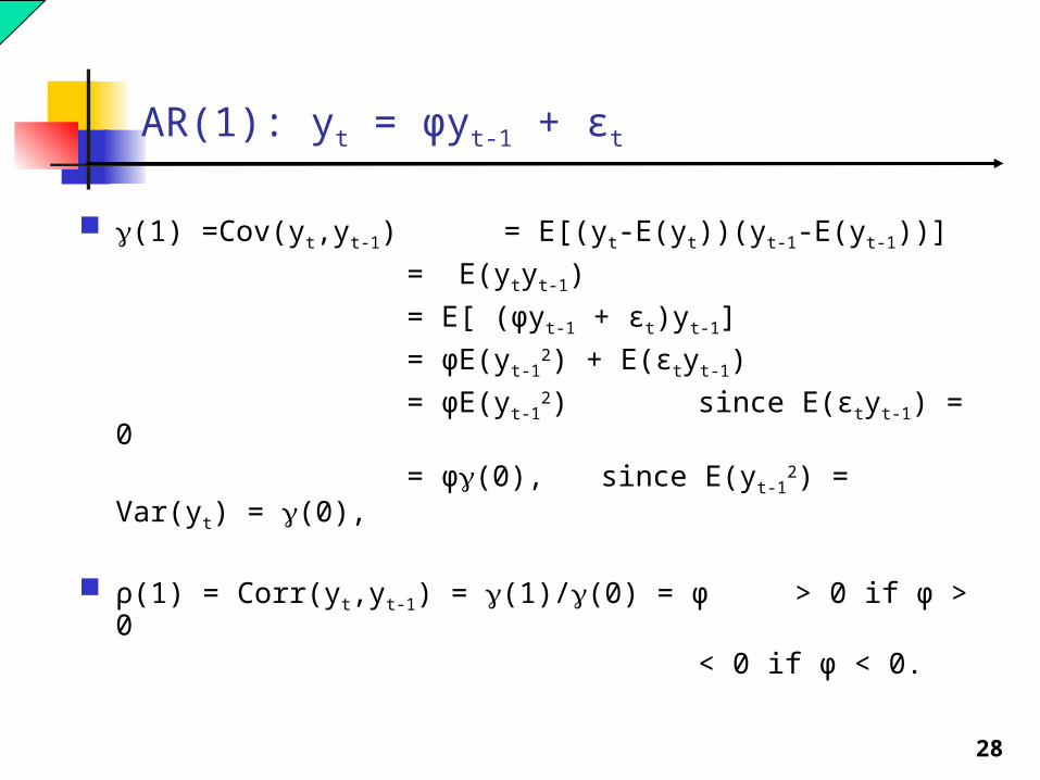
AR(1): yt = φyt-1 + εt
(1) =Cov(yt,yt-1) = E[(yt-E(yt))(yt-1-E(yt-1))]
= E(ytyt-1)
= E[ (φyt-1 + εt)yt-1]
= φE(yt-12) + E(εtyt-1)
= φE(yt-12) since E(εtyt-1) = 0
= φ(0), since E(yt-12) = Var(yt) =
(0),
ρ(1) = Corr(yt,yt-1) = (1)/(0) = φ > 0 if φ > 0 < 0 if φ < 0.

29
AR(1): yt = φyt-1 + εt
More generally, for the AR(1) process: ρ() = φ for all
So the ACF for the AR(1) process will Be nonzero for all values of , decreasing monotonically
in absolute value to zero as increases be strictly positive, decreasing monotonically to zero as
increases, if φ is positive alternate in sign as it decreases to zero, if φ is negative
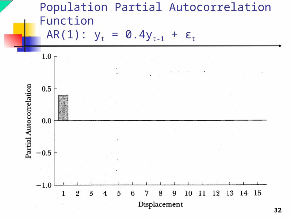
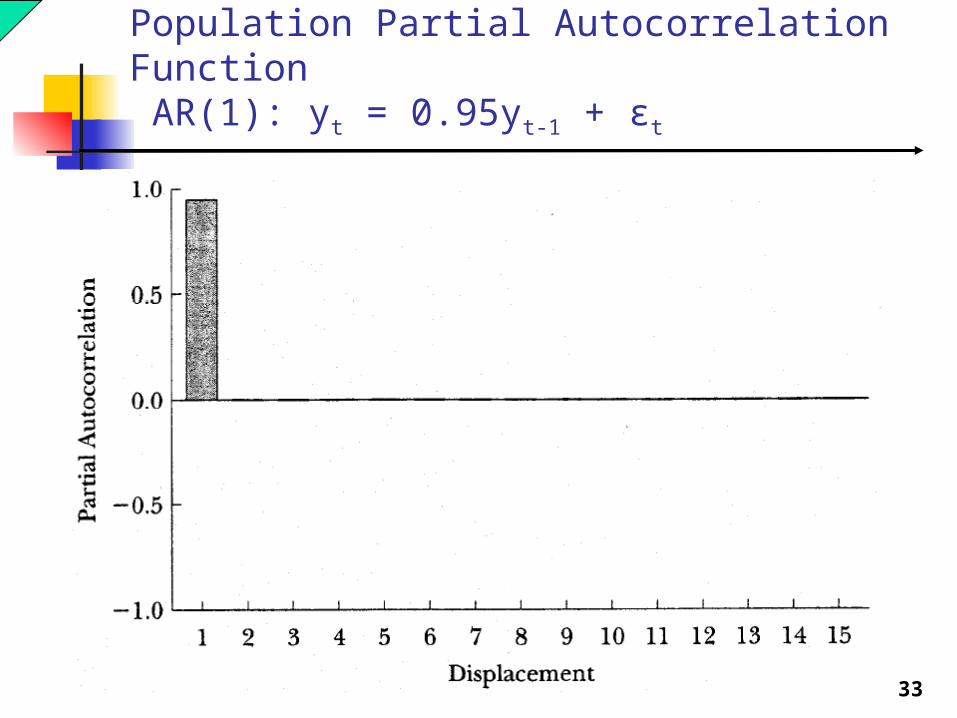
The PACF for an AR(1)will be equal to φ for = 1 and will be equal to 0 otherwise, i.e.,
p() = φ if = 1 0 if > 1
30
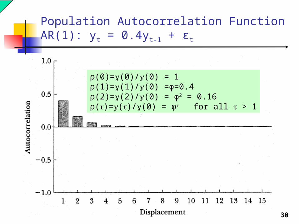
Population Autocorrelation FunctionAR(1): yt = 0.4yt-1 + εt
ρ(0)=(0)/(0) = 1ρ(1)=(1)/(0) =φ=0.4ρ(2)=(2)/(0) = φ2 = 0.16ρ()=()/(0) = φ for all > 1

31
Population Autocorrelation Function AR(1): yt = 0.95yt-1 + εt
ρ(0)=(0)/(0) = 1ρ(1)=(1)/(0) =φ=0.95ρ(2)=(2)/(0) = φ2 = 0.9025ρ()=()/(0) = φ for all > 1
32
Population Partial Autocorrelation Function AR(1): yt = 0.4yt-1 + εt
33
Population Partial Autocorrelation Function AR(1): yt = 0.95yt-1 + εt

34
AR(1): yt = φyt-1 + εt
E(yT+h│yT,yT-1,…)= E(yT+h│yT,yT-1,… εT,εT-1,…)
1. E(yT+1│yT,yT-1,…, εT,εT-1,…) = E(φyT+εT+1│ yT,yT-1,…, εT,εT-1,…)= E(φyT │ yT,yT-1,…, εT,εT-1,…) + E(εT+1│ yT,yT-1,…, εT,εT-1,…)= φyT
2. E(yT+2│ yT,yT-1,…, εT,εT-1,…)= E(φyT+1+εT+2│ yT,yT-1,…, εT,εT-1,…)= E(φyT+1│yT,yT-1,…, εT,εT-1,…)= φ E(yT+1│yT,yT-1,…, εT,εT-1,…)= φ(φyT) = φ2yT
3. E(yT+h│yT,yT-1,…) = φhyT

35
Properties of the AR(p) Process
yt = φ1yt-1+ φ2yt-2+…+ φpyt-p+εt
or, using the lag operator,φ(L)yt = εt, φ(L) = 1- φ1L-…-φpLp
where the ε’s are WN(0,σ2).

36
AR(p): yt = φ1yt-1+ φ2yt-2+…+ φpyt-p+εt
The coefficients of the AR(p) model of a covariance stationary time series must satisfy the stationarity condition: Consider the values of x that solve the equation
1-φ1x-…-φpxp = 0
These x’s must all be greater than 1 in absolute value.
For example, if p = 1 (the AR(1) case), consider the solutions to
1- φx = 0The only value of x that satisfies this equation is x = 1/φ, which will be greater than one in absolute value if and only if the absolute value of φ is less than one. So, │φ│< 1 is the stationarity condition for the AR(1) model.The condition guarantees that the impact of εt on yt+
decays to zero as increases.

37
AR(p): yt = φ1yt-1+ φ2yt-2+…+ φpyt-p+εt
The autocovariance and autocorrelation functions, () and ρ(), will be non-zero for all . Their exact shapes will depend upon the signs and magnitudes of the AR coefficients, though we know that they will be decaying to zero as goes to infinity.
The partial autocorrelation function, p(), will be equal to 0 for all > p.
The exact shape of the pacf for 1 < < p will depend on the signs and magnitudes of φ1,…, φp.

38
Population Autocorrelation Function AR(2): yt = 1.5yt-1 -0.9yt-2+ εt

39
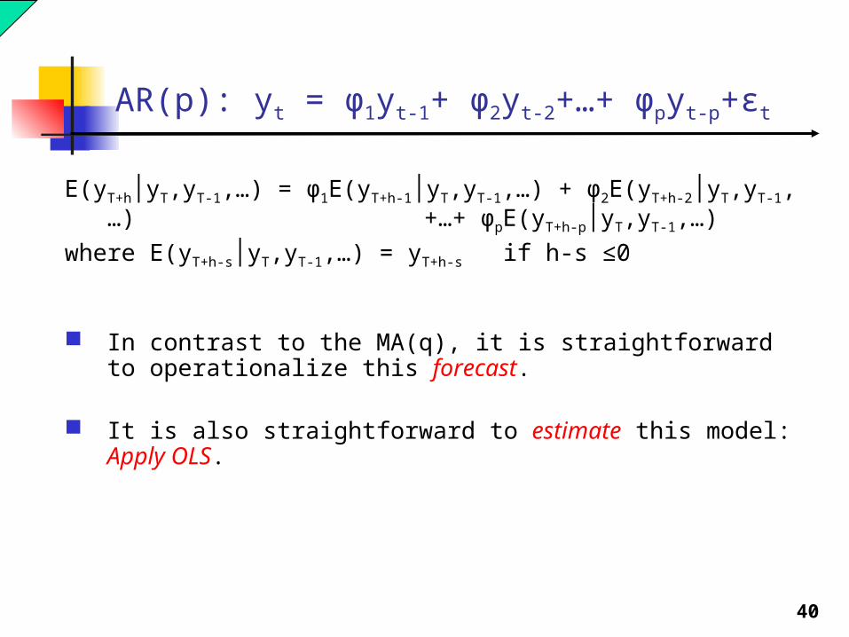
AR(p): yt = φ1yt-1+ φ2yt-2+…+ φpyt-p+εt
E(yT+h│yT,yT-1,…) = ? h = 1:
yT+1 = φ1yT+ φ2yT-1+…+ φpyT-p+1+εT+1
E(yT+1│yT,yT-1,…)=φ1yT+φ2yT-1+…+φpyT-p+1
h = 2:yT+2 = φ1yT+1+ φ2yT+…+ φpyT-p+2+εT+2
E(yT+2│yT,yT-1,…) = φ1E(yT+1│yT,yT-1,…) + φ2yT+…+ φpyT-p+2
h = 3yT+3 = φ1yT+2+ φ2yT+1+ φ3yT+…+ φpyT-p+3+εT+3
E(yT+3│yT,yT-1,…) = φ1E(yT+2│yT,yT-1,…) + φ2E(yT+1│yT,yT-1,…) + φ3yT+…+ φpyT-p+3
40
AR(p): yt = φ1yt-1+ φ2yt-2+…+ φpyt-p+εt
E(yT+h│yT,yT-1,…) = φ1E(yT+h-1│yT,yT-1,…) + φ2E(yT+h-2│yT,yT-1,…) +…+ φpE(yT+h-p│yT,yT-1,…)
where E(yT+h-s│yT,yT-1,…) = yT+h-s if h-s ≤0
In contrast to the MA(q), it is straightforward to operationalize this forecast.
It is also straightforward to estimate this model: Apply OLS.
41
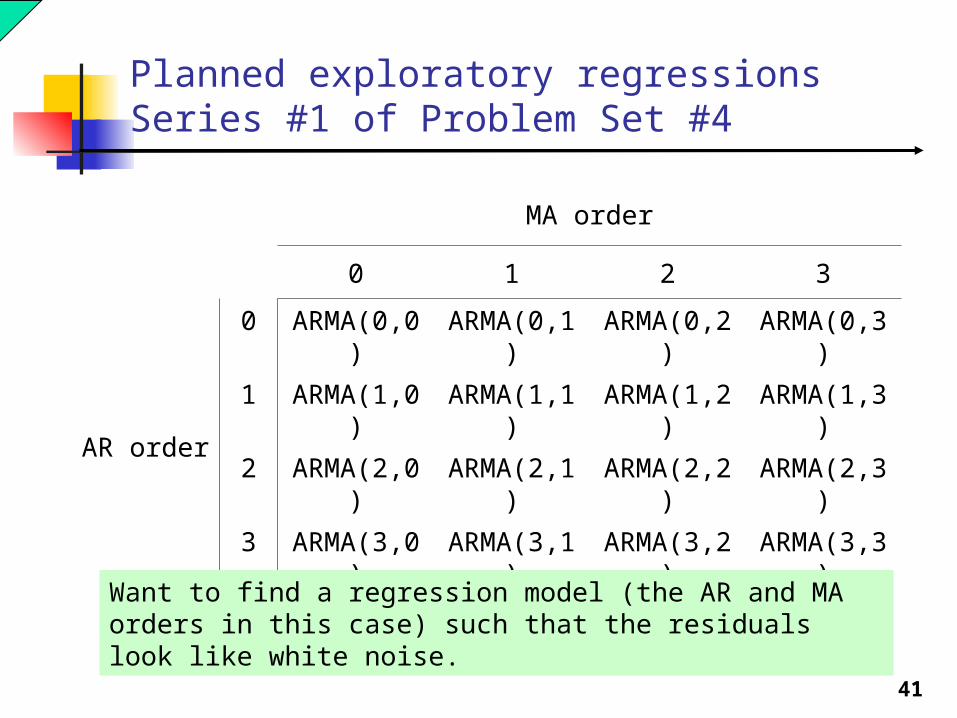
Planned exploratory regressions Series #1 of Problem Set #4
MA order
0 1 2 3
AR order
0 ARMA(0,0)
ARMA(0,1)
ARMA(0,2)
ARMA(0,3)
1 ARMA(1,0)
ARMA(1,1)
ARMA(1,2)
ARMA(1,3)
2 ARMA(2,0)
ARMA(2,1)
ARMA(2,2)
ARMA(2,3)
3 ARMA(3,0)
ARMA(3,1)
ARMA(3,2)
ARMA(3,3)
Want to find a regression model (the AR and MA orders in this case) such that the residuals look like white noise.

42
Model selection
MA order
0 1 2 3
AR order
0 3.062311
2.833607
2.804140
2.798167
1 2.785920
2.790444
2.793938
2.798289
2 2.791028
2.779683
2.784112
2.786560
3 2.795964
2.783694
2.782536
2.786013
MA order
0 1 2 3
AR order
0 3.071552
2.852088
2.831862
2.835130
1 2.804432
2.818213
2.830964
2.844570
2 2.818845
2.816772
2.830473
2.842193
3 2.833116
2.830135
2.838265
2.851030
AIC
SIC
43
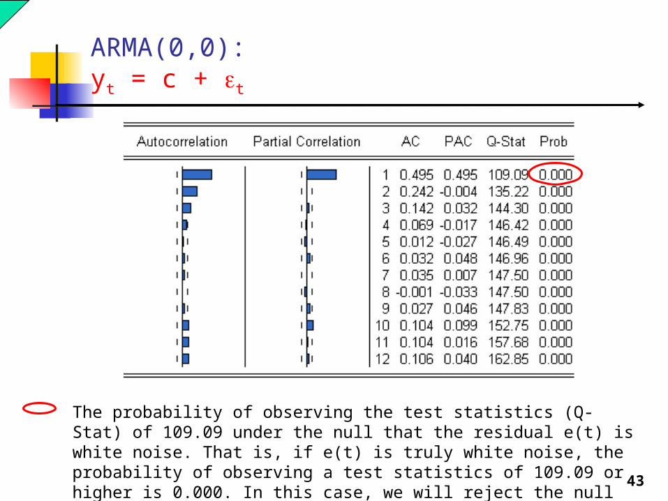
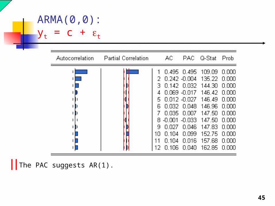
ARMA(0,0): yt = c + t
The probability of observing the test statistics (Q-Stat) of 109.09 under the null that the residual e(t) is white noise. That is, if e(t) is truly white noise, the probability of observing a test statistics of 109.09 or higher is 0.000. In this case, we will reject the null hypothesis.

44
ARMA(0,0): yt = c + t
The 95% confidence band for the autocorrelation under the null that residuals e(t) is white noise. That is, if e(t) is truly white noise, 95% of time (out of many realization of samples), the autocorrelation will fall within the band. We will reject the null hypothesis if the autocorrelation falls outside the band.
45
ARMA(0,0): yt = c + t
The PAC suggests AR(1).

46
ARMA(0,1)
47
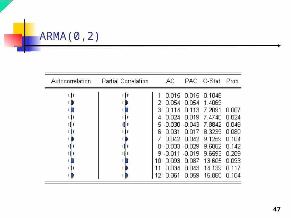
ARMA(0,2)
48
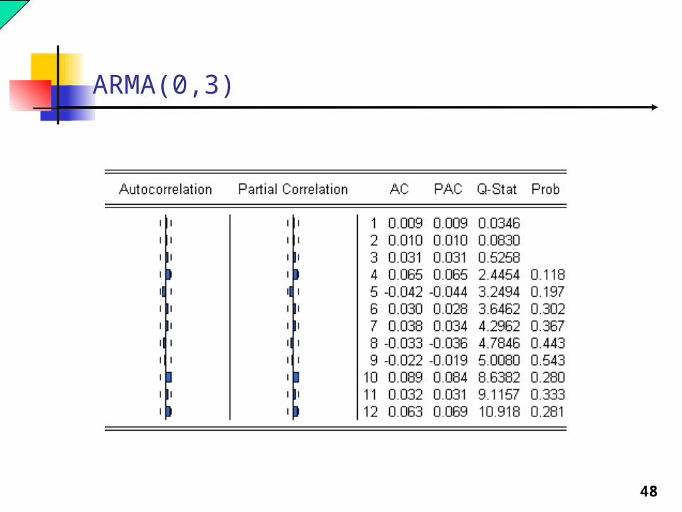
ARMA(0,3)

49
ARMA(1,0)
50
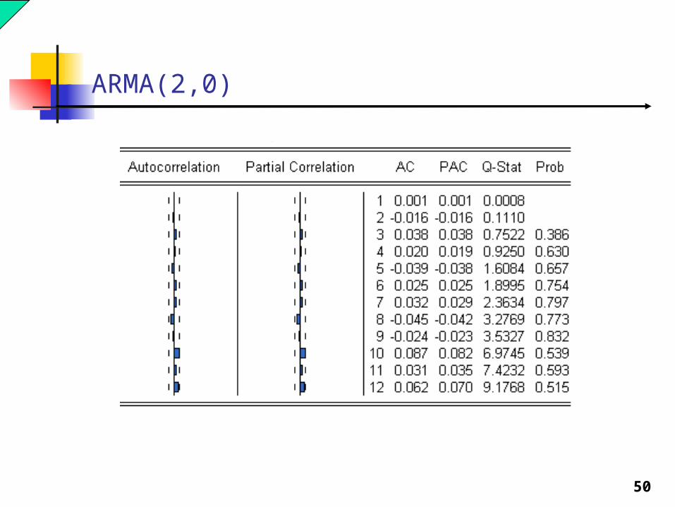
ARMA(2,0)

51
ARMA(1,1)

52
AR or MA?
ARMA(1,0) ARMA(0,3)
Truth: yt = 0.5 yt-1 + t
We cannot reject the null that e(t) is white noise in both models.
53
Approximation
Any MA process may be approximated by an AR(p) process, for sufficient large p. And the residuals will appear white noise.
Any AR process may be approximated by a MA(q) process, for sufficient large q. And the residuals will appear white noise.
In fact, if an AR(p) process can be written exactly as a MA(q) process, the AR(p) process is called invertible.
Similarly, if a MA(q) process can be written exactly as an AR(p) process, the MA(q) process is called invertible.
54
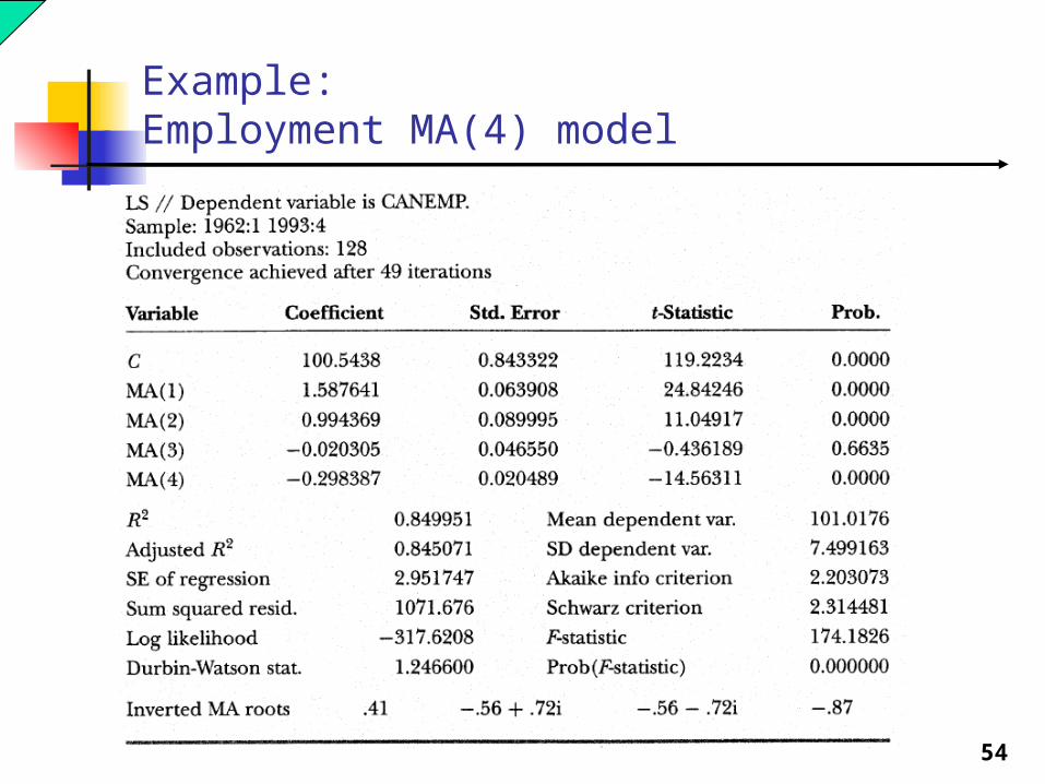
Example:Employment MA(4) model
55
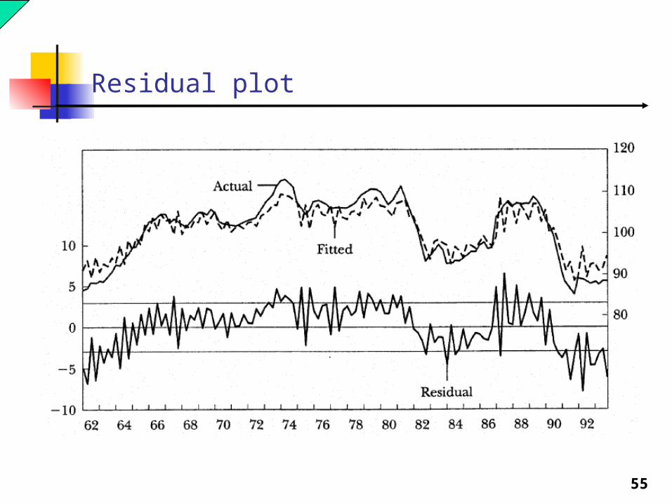
Residual plot

56
Correlogram of sample residual from an MA(4) model
57
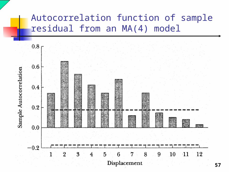
Autocorrelation function of sample residual from an MA(4) model

58
Partial autocorrelation function of sample residual from an MA(4) model
59
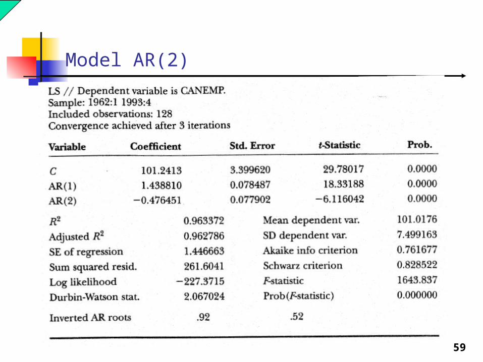
Model AR(2)
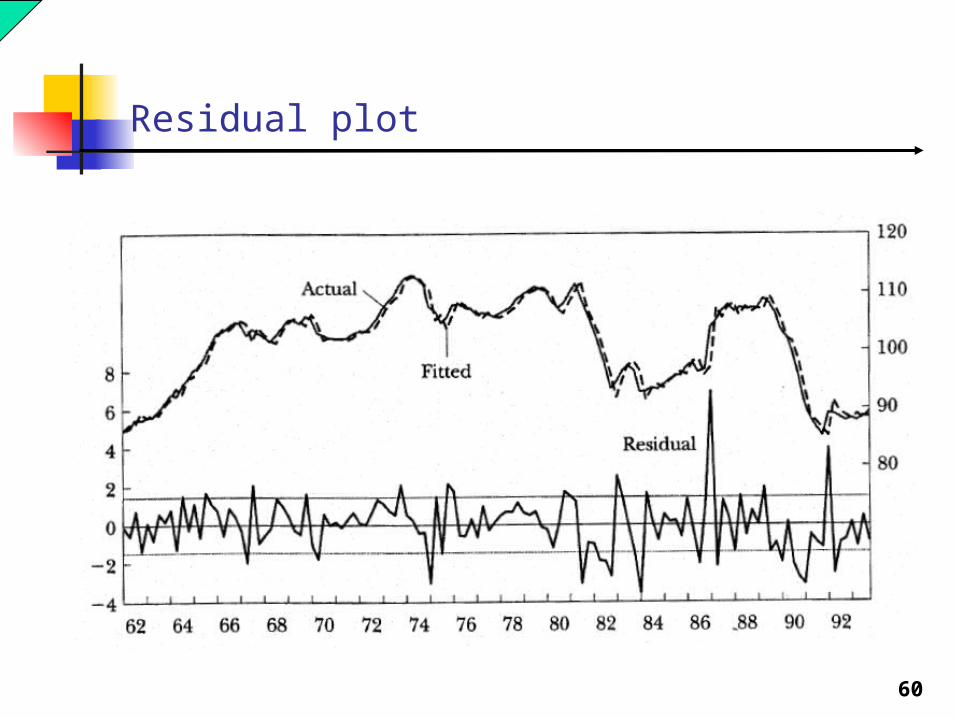
60
Residual plot
61
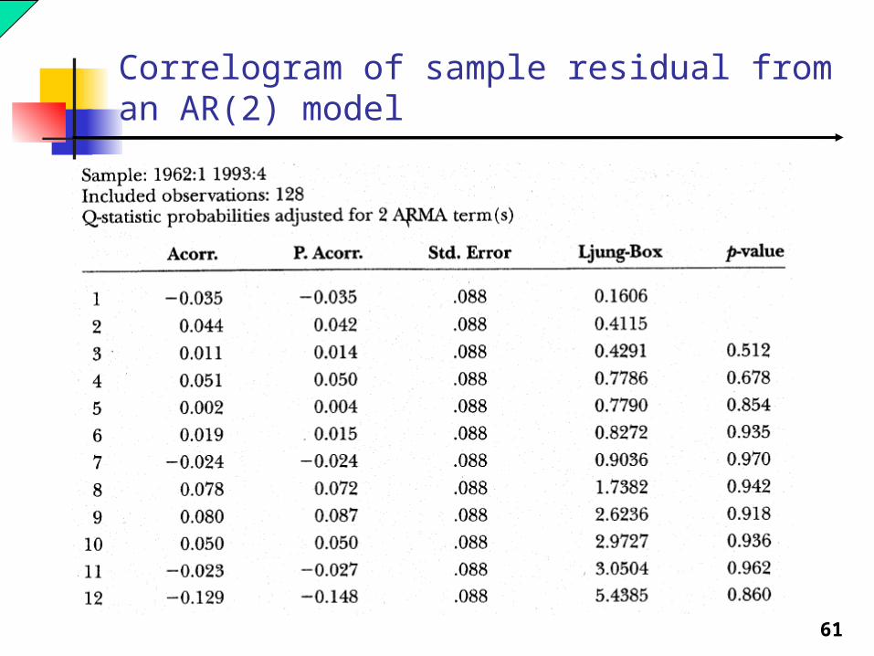
Correlogram of sample residual from an AR(2) model

62
Model selection criteria – various MA and AR orders
SIC values
AIC values

63
Autocorrelation function of sample residual from an AR(2) model
64
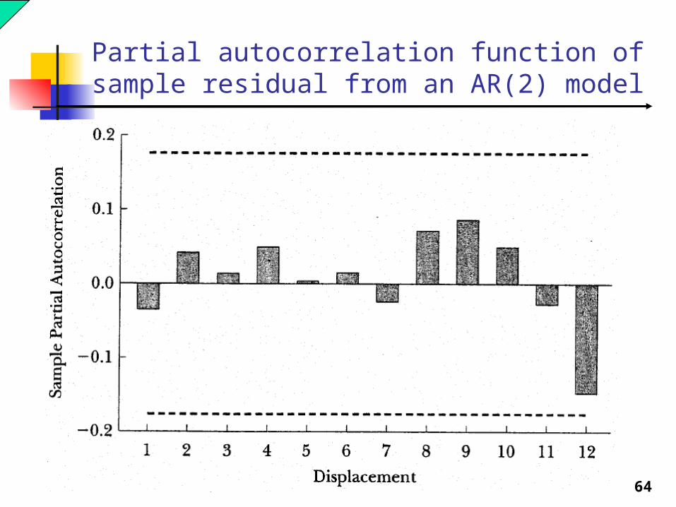
Partial autocorrelation function of sample residual from an AR(2) model

65
ARMA(3,1)

66
Residual plot
67
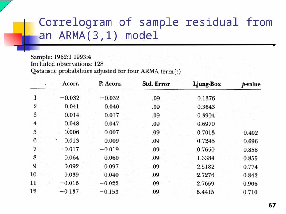
Correlogram of sample residual from an ARMA(3,1) model

68
Autocorrelation function of sample residual from an ARMA(3,1) model

69
Partial autocorrelation function of sample residual from an ARMA(3,1) model
70
End