1 lecture 21, statistics 246, april 8, 2004 identifying expression differences in cdna microarray...
Post on 21-Dec-2015
217 views
TRANSCRIPT

1
Lecture 21, Statistics 246,April 8, 2004
Identifying expression differences in cDNA microarray experiments, cont.

2
An empirical Bayes story
Suppose that our M values are independently and normally distributed, and that a proportion p of genes are differentially expressed, i.e. have M’s with non-zero means.
Further, suppose that the variances and means of these are chosen jointly
from inverse chi-square and normal conjugate priors, respectively. Genes not differentially expressed have zero means, and variances chosen
from the same inverse chi-squared distribution. The scale and d.f. parameters in the inverse chi-square are estimated from
the data, as is a parameter c connecting the prior for the mean with that for the variances.
We then calculate for the posterior probability that a given gene is
differentially expressed, and find it is an increasing function of B over the page, where a and c are estimated parameters, and p is in the constant.

3
B=const+log
2an
+s2 +M•2
2an
+s2 +M•
2
1+nc
⎛
⎝
⎜ ⎜
⎞
⎠
⎟ ⎟
Empirical Bayes log posterior odds ratio (LOR)
Notice that for large n this approximately t=M./s .

4
B=LOR compared with t and M.

5
Extensions include dealing with
• Replicates within and between slides• Several effects: use a linear model• ANOVA: are the effects equal?• Time series: selecting genes for trends
6
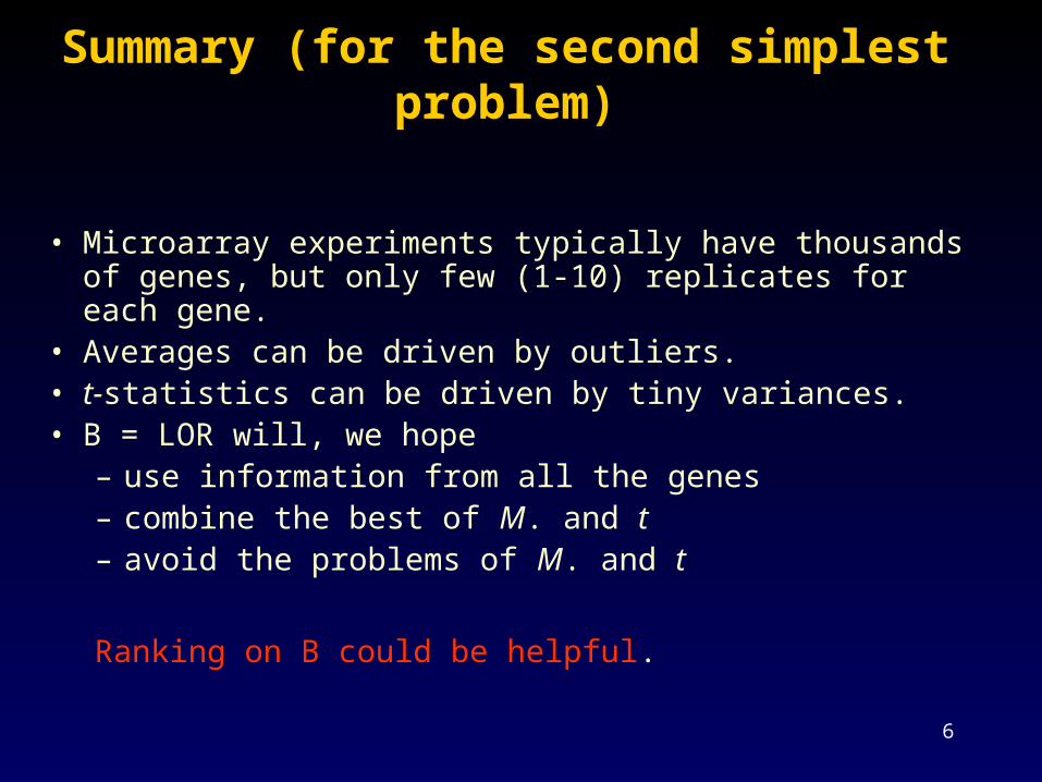
Summary (for the second simplest problem)
• Microarray experiments typically have thousands of genes, but only few (1-10) replicates for each gene.
• Averages can be driven by outliers.• t-statistics can be driven by tiny variances.• B = LOR will, we hope
– use information from all the genes– combine the best of M. and t– avoid the problems of M. and t
Ranking on B could be helpful.

7
Use of linear models with cDNA microarray data
In many situations we want to combine data from different experiments in a slightly more elaborate manner than simply averaging. One way of doing so is via (fixed effects) linear models, where we estimate certain quantities of interest which we call effects for each gene on our slide.
Typically these estimates may be regarded as approximately normally distributed with common SD, and mean zero in the absence of any relevant differential expression.
In such cases, the preceding two strategies: qq-plots, and various combinations of estimated effect (cf M.), standardized estimate (cf. t) both apply.

8
Advantages of linear models
• Analyse all arrays together combining information in optimal way
• Combined estimation of precision• Extensible to arbitrarily complicated experiments• Design matrix: specifies RNA targets used on
arrays• Contrast matrix: specifies which comparisons
are of interest

9
Log-ratios or single channel intensities?
• Traditional analyses, as here, treat log-ratios M=log(R/G) as the primary data, i.e., we take gene expression measurements as relative
• An alternative approach treats individual channel intensities R and G as the primary data, i.e., views gene expression measures as “absolute” (Wolfinger, Churchill, Kerr)
• A single channel approach makes new analyses possible but it– make stronger assumptions– requires more complex models (mixed models in
place of ordinary linear models) to accommodate correlation between R and G on same spot
– requires absolute normalization methods
10
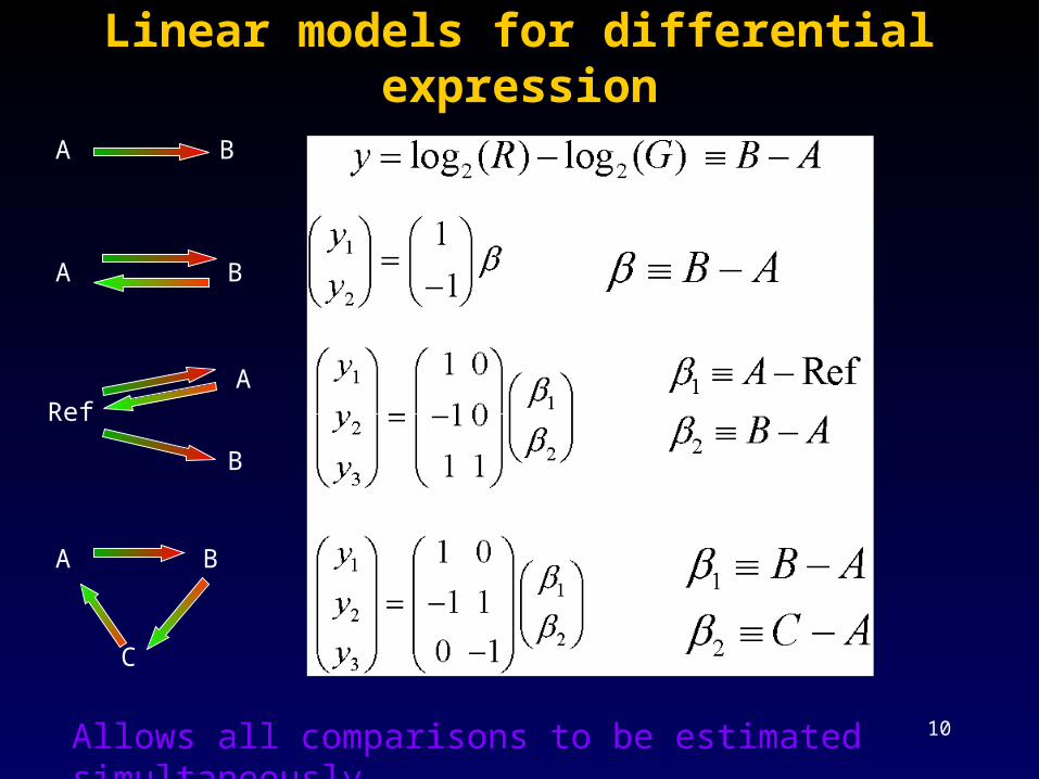
Linear models for differential expression
A B
RefA
B
A B
A B
C
Allows all comparisons to be estimated simultaneously
11
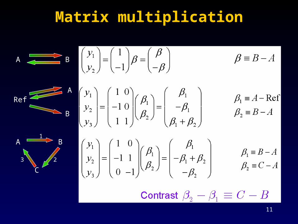
Matrix multiplication
A B
RefA
B
A B
C
1
23

12
⎟⎟⎟⎟⎟⎟
⎠
⎞
⎜⎜⎜⎜⎜⎜
⎝
⎛
⎥⎥⎥⎥⎥⎥⎥⎥⎥
⎦
⎤
⎢⎢⎢⎢⎢⎢⎢⎢⎢
⎣
⎡
=
⎟⎟⎟⎟⎟⎟⎟⎟⎟
⎠
⎞
⎜⎜⎜⎜⎜⎜⎜⎜⎜
⎝
⎛
ba
ba
b
a
a
y
y
y
y
y
y
y
2
1
2
1
7
6
5
4
3
2
1
11100
10010
00010
01100
01001
00001
00100
WT.P11 + a1
MT.P21 + (a1 + a2) + b + (a1 + a2)b
MT.P11 +a1+b+a1.b
WT.P21 + a1 + a2
WT.P1
MT.P1 + b
1
2
3
4
5
6
7
Slightly larger example:

13
Linear model estimates
Obtain a linear model for each gene g
Estimate model by robust regression,least squares or generalized least squaresto get
coefficients
standard deviations
standard errors

14
Parallel inference for genes
• 10,000-40,000 linear models• Curse of dimensionality:
Need to adjust for multiple testing, e.g., control family-wise error rate (FWE) or false discovery rate (FDR)
• Boon of parallelism:Can borrow information from one gene to another

15
Hierarchical model
Normal Model Prior
Normality, independence assumptions are wrong but convenient, resulting methods are useful
16
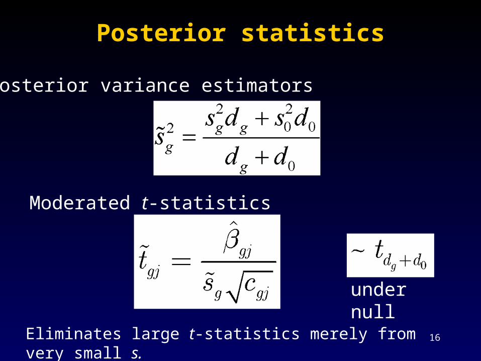
Posterior statistics
Moderated t-statistics
Posterior variance estimators
Eliminates large t-statistics merely from very small s.
under null

17
Posterior Odds
Posterior probability of differential expression for any gene is
Generalization of B mentioned earlier.
Monotonic function of for constant d.
Exercise. Prove all the distributional statements made above.

18
Summary
• Analyse data all at once
• Use standard deviances not just fold changes
• Use ensemble information to shrink variances
• Assess differential expression for all comparisons together

19
Appendix: slightly more general theoretical development
Assume that for each gene,
Also, assume that certain contrasts g = CT g are of interest. The estimators of these contrasts and their estimated covariance matrices are
If we let vgj be the jth diagonal element of CTVgC, then our assumptions are
where dg is the residual degrees of freedom in the linear model for gene g.
€
E(yg ) = Xα g; var(yg ) =Wgσ g2 .
€
) g =CT
) α g , var(
) β g ) =CTVgCσ g
2.
€
) gj | β gj ,σ g
2 ~ N(β gj ,vgjσ g2), sg
2 |σ g2 ~
σ g2
dgχ dg
2 ,

20
Hierarchical model
As before, we define a simple hierarchical model to combine information across the genes. Prior information on the variances is assumed to come via a prior estimate 2 with d.f. :
For any given j, we assume gj non-zero with known proportion pj
pr(gj 0) = pj .For those genes which are differentially expressed, prior information is assumed in the form
The moderated t and posterior odds are as before. See http://bioinf.wehi.edu.au/limma/ for an R-package and more details.
€
1
σ g2
~1
νλ 2χ ν
2 .
€
) gj |σ g
2,β gj ≠ 0 ~ N(0,λ jσ g2).

21
From single genes to sets of genes
All of the foregoing has concerned single genes, i.e. has been a one-gene-at-a-time approach, although the empirical Bayes idea exploits the fact that there are really lots of genes.
The problem of discovering sets of genes affected by a treatment at the same time as carrying out some kind of statistical inference, remains a challenge.
What follows is a quick reminder that many people use clustering in this context, sometimes ignoring known information about the units being clustered. What is relevant here is that clustering can deliver sets of genes associated with treatment or other differences, though not to date within a formal statistical framework.
We then present a brief discussion of a related idea, aimed at finding sets of genes which can be examined in much the same way as single genes.

22
Cluster Analysis
Can cluster genes, cell samples, or both.
Strengthens signal when averages are taken within clusters of genes (Eisen).
Useful (essential ?) when seeking new subclasses of cells, tumours, etc.
Leads to readily interpreted figures.

23
Clusters
Taken from Nature February, 2000Paper by Allzadeh. A et alDistinct types of diffuse large B-cell lymphoma identified by Gene expression profiling,

24
Discovering sub-groups

25
Limitations
Cluster analyses:1) Usually outside the normal framework of statistical
inference;2) less appropriate when only a few genes are likely to
change.3) Needs lots of experimentsSingle gene tests:1) may be too noisy in general to show much2) may not reveal coordinated effects of positively
correlated genes.3) hard to relate to pathways.

26
A synthesis
We and others are working on methods which try to combine the best of both of the preceding approaches.
Try to find groups of genes and combine their responses to reduce noise and enhance interpretability.
Use testing to assign significance with groups of genes as we did with single genes.

27
One approach: clustering genes
1 2 3 4 5
Cluster 6=(1,2)
Cluster 7=(1,2,3)Cluster 8=(4,5)
Cluster 9= (1,2,3,4,5)
Let p = number of genes.
1. Calculate within class correlation.
2. Perform hierarchical clustering which will produce (2p-1) clusters of genes.
3. Average within clusters of genes.
4 Perform testing on averages of clusters of genes as if they were single genes.
E.g. p=5

28
Data - Ro1
Transgenic mice with a modified Gi coupled receptor (Ro1).
Experiment: induced expression of Ro1 in mice.8 control (ctl) mice 9 treatment mice eight weeks after Ro1 being induced. Long-term question: Which groups of genes work
together. Based on paper: Conditional expression of a Gi-coupled
receptor causes ventricular conduction delay and a lethal cardiomyopathy, see Redfern C. et al. PNAS, April 25, 2000.
http://www.pnas.org alsohttp://www.GenMAPP.org/ (Conklin lab, UCSF)

29
Histogram
Cluster of genes(1703, 3754)

30
Top 15 averages of gene clusters
-13.4 7869 = (1703, 3754)
-12.1 3754
11.8 6175
11.7 4689
11.3 6089
11.2 1683
-10.7 2272
10.7 9955 = (6194, 1703, 3754)
10.7 5179
10.6 3916
-10.4 8255 = (4572, 4772, 5809)
-10.4 4772
-10.4 10548 = (2534, 1343, 1954)
10.3 9476 = (6089, 5455, 3236, 4014)
Might be influenced by 3754
1 0.7 0.7
0.7 1 0.8
0.7 0.8 1
⎡
⎣
⎢ ⎢
⎤
⎦
⎥ ⎥
Correlation1 0.5 0.5
0.5 1 0.8
0.5 0.8 1
⎡
⎣
⎢ ⎢
⎤
⎦
⎥ ⎥
T Group ID

31
Remarks
Hard to extend this method to negatively correlated clusters of genes. Need to consider together with other methods.
Need to identify high averages of clusters of genes that are due to high averages from sub-clusters of those genes.
May be worth pursuing. Not clear.
32
Acknowledgments
Yee Hwa Yang
Sandrine Dudoit
Ingrid Lönnstedt
Natalie Thorne
David Freedman
Gordon Smyth
Ngai lab, UCB
Matt Callow (LBNL)
Bruce Conklin
Karen Vranizan