1 mil gold bond wire study...sandia report sand2013-3715 unlimited release printed may 2013 1 mil...
TRANSCRIPT

SANDIA REPORT SAND2013-3715 Unlimited Release Printed May 2013
1 Mil Gold Bond Wire Study Johnathon D. Huff, Michael B. McLean, Mark W. Jenkins, and Brian M. Rutherford Prepared by Sandia National Laboratories Albuquerque, New Mexico 87185 and Livermore, California 94550
Sandia National Laboratories is a multi-program laboratory managed and operated by Sandia Corporation, a wholly owned subsidiary of Lockheed Martin Corporation, for the U.S. Department of Energy's National Nuclear Security Administration under contract DE-AC04-94AL85000. Approved for public release; further dissemination unlimited.

2
Issued by Sandia National Laboratories, operated for the United States Department of Energy by Sandia Corporation. NOTICE: This report was prepared as an account of work sponsored by an agency of the United States Government. Neither the United States Government, nor any agency thereof, nor any of their employees, nor any of their contractors, subcontractors, or their employees, make any warranty, express or implied, or assume any legal liability or responsibility for the accuracy, completeness, or usefulness of any information, apparatus, product, or process disclosed, or represent that its use would not infringe privately owned rights. Reference herein to any specific commercial product, process, or service by trade name, trademark, manufacturer, or otherwise, does not necessarily constitute or imply its endorsement, recommendation, or favoring by the United States Government, any agency thereof, or any of their contractors or subcontractors. The views and opinions expressed herein do not necessarily state or reflect those of the United States Government, any agency thereof, or any of their contractors. Printed in the United States of America. This report has been reproduced directly from the best available copy. Available to DOE and DOE contractors from U.S. Department of Energy Office of Scientific and Technical Information P.O. Box 62 Oak Ridge, TN 37831 Telephone: (865) 576-8401 Facsimile: (865) 576-5728 E-Mail: [email protected] Online ordering: http://www.osti.gov/bridge Available to the public from U.S. Department of Commerce National Technical Information Service 5285 Port Royal Rd. Springfield, VA 22161 Telephone: (800) 553-6847 Facsimile: (703) 605-6900 E-Mail: [email protected] Online order: http://www.ntis.gov/help/ordermethods.asp?loc=7-4-0#online

3
SAND2013-3715 Unlimited Release Printed May 2013
1 Mil Gold Bond Wire Study
Johnathon D. Huff and Michael B. McLean Use Control Systems Department
Mark W. Jenkins
Validation and Failure Analysis Department
Brian M. Rutherford Human Factors and Statistics Department
Sandia National Laboratories
P.O. Box 5800 Albuquerque, New Mexico 87185-MS1206
Abstract
In microcircuit fabrication, the diameter and length of a bond wire have been shown to both affect the current versus fusing time ratio of a bond wire as well as the gap length of the fused wire. This study investigated the impact of current level on the time-to-open and gap length of 1 mil by 60 mil gold bond wires. During the experiments, constant current was provided for a control set of bond wires for 250ms, 410ms and until the wire fused; non-destructively pull-tested wires for 250ms; and notched wires. The key findings were that as the current increases, the gap length increases and 73% of the bond wires will fuse at 1.8A, and 100% of the wires fuse at 1.9A within 60ms. Due to the limited scope of experiments and limited data analyzed, further investigation is encouraged to confirm these observations.

4
ACKNOWLEDGMENTS The authors would like to thank Kenneth C. Chen of Sandia National Laboratories for discussions on test planning and data interpretation. The authors also acknowledge the valuable contributions of James “Jim” A. Woods III and Brian Wroblewski of Sandia National Laboratories for their work building the test vehicles.

5
CONTENTS
Acknowledgments........................................................................................................................... 4
Contents .......................................................................................................................................... 5
Figures............................................................................................................................................. 6
Tables .............................................................................................................................................. 6
1. Introduction ............................................................................................................................. 7
2. Test Units .............................................................................................................................. 10
3. Test Equipment Configuration .............................................................................................. 12 3.1. Length Calculations ...................................................................................................... 14
4. Test Procedures and Results ................................................................................................. 16 4.1. Test No. 1A: Constant Current at Fixed Pulse Width (250ms) .................................... 16
4.1.1. Test Procedure Overview ................................................................................ 16 4.1.2. Test Results ..................................................................................................... 16
4.2. Test No. 1B: Constant Current at Fixed Pulse Width (410ms) ..................................... 19 4.2.1. Test Procedure Overview ................................................................................ 19 4.2.2. Test Results ..................................................................................................... 19
4.3. Test No. 1C: Constant Current (2A – 6A) .................................................................... 20 4.3.1. Test Procedure ................................................................................................ 21 4.3.2. Test Results ..................................................................................................... 21
4.4. Test No. 2: Constant Current at Fixed Pulse Width (Pull-tested Bond Wires) ............. 24 4.4.1. Test Procedure ................................................................................................ 24 4.4.2. Test Results ..................................................................................................... 24
4.5. Test No. 3: Constant Current at Fixed Pulse Width on Notched Wires ....................... 25 4.5.1. Test Procedure ................................................................................................ 26 4.5.2. Test Results ..................................................................................................... 26
5. Conclusions ........................................................................................................................... 28 5.1. Key Results ................................................................................................................... 28 5.2. Future Work .................................................................................................................. 28
6. References ............................................................................................................................. 30
Appendix A – Test No. 1A Data ................................................................................................... 32
Appendix B – Test No. 1B Data ................................................................................................... 34
Appendix C – Test No. 1C Data ................................................................................................... 35
Appendix D – Test No. 2 Data...................................................................................................... 36
Appendix E – Statistical Testing................................................................................................... 37
Appendix F – Computation of Statistical Tolerance Limits ......................................................... 41
Distribution ................................................................................................................................... 45

6
FIGURES Figure 1. Schematic of Bond Wire [5] ............................................................................................ 7 Figure 2. Test Vehicle with 45 Bonds (4 ½ x 4 ½ in.) .................................................................. 10 Figure 3. Test Vehicle Bond Wire Pad Design ............................................................................. 10 Figure 4. Scanning Electron Microscope (SEM) Image (a); Optical Image (b) ........................... 11 Figure 5. Constant Current Test Circuit ........................................................................................ 12 Figure 6. Green Trace Shows No Melting (a); Green Trace Shows Melting at 31ms (b) ............ 13 Figure 7. Test Set-up Switching Equipment on Left, Thermal Imaging Equipment on Right ..... 13 Figure 8. Thermal Imaging of One Wire Bond on Test Vehicle with Current Provided by Probes....................................................................................................................................................... 14 Figure 9. Reference Measurement ................................................................................................ 14 Figure 10. Gap Length Measurement (16.9 mil) .......................................................................... 16 Figure 11. 1.7A, Fused at 170s, Gap Length = 3.54 mil ............................................................... 17 Figure 12. 1.8A, Fused at 126s, Gap Length = 3.15 mil ............................................................... 17 Figure 13. 1.9A, Fused at 28s, Gap Length = 3.94 mil ................................................................. 18 Figure 14. Current vs. Gap Length ............................................................................................... 21 Figure 15. 2A, Fused at 9.4ms, GAP Length = 5.31 mil .............................................................. 21 Figure 16. 3A, Fused at 2.9ms, Gap Length = 10.94 mil ............................................................. 22 Figure 17. 4A, Fused at 1.6ms, Gap Length = 16.9 mil ............................................................... 22 Figure 18. 5A, Fused at 0.92ms, Gap Length = 28.7 mil ............................................................. 22 Figure 19. 6A, Fused at 0.69ms, Gap Length = 31.4 mil ............................................................. 23 Figure 20. Current vs. Gap Length ............................................................................................... 23 Figure 21. Pull vs. Non-pull Tested .............................................................................................. 24 Figure 22. Bond Wire with 25% Notch ........................................................................................ 25 Figure F1. 1.8A Censored Data .................................................................................................... 41 Figure F2. 1.8A Data .................................................................................................................... 42 Figure F3. 1.9A Censored Data .................................................................................................... 42 Figure F4. 1.9A Data .................................................................................................................... 43
TABLES
Table 1. Results Summary .............................................................................................................. 8 Table 2. Fusing Current Results Summary (250ms) ..................................................................... 16 Table 3. Fusing Current Results Summary (410ms) ..................................................................... 19 Table 4. Log-normal Distribution Parameters .............................................................................. 19 Table 5. Tolerance Bounds ........................................................................................................... 20 Table 6. Fusing Current Results Summary (Pull-tested) .............................................................. 24 Table 7. Estimate for Distribution of Fusing Times ..................................................................... 25 Table 8. Fusing Current with Notched Wires Results Summary .................................................. 26 Table 9. Future Work Summary ................................................................................................... 28

7
1. INTRODUCTION Wire fusing is one of the important sources of circuit failures in microelectronics. Bond wires made of gold are common. Gold bond wire fusing is dominated by heat conduction through the wire. The ends of each wire are connected to a heat sink and maintained at a low temperature [1], [2]. The maximum temperature then occurs at the center of the wire. Before melting occurs at the wire center, the one-dimensional heat equation can be solved [Error! Bookmark not defined.], [3]. The calculated threshold values are found to be approximately 15% lower than the measured value. After the wire center begins to melt, capillary action dominates; Lord Rayleigh determined that maximum instability occurs at a fused (gap) length of 4.51d [7], where d is the wire diameter. This value will be used as the minimum fused (gap) length. The solution to the one-dimensional heat equation given in [Error! Bookmark not defined.], [Error! Bookmark not defined.] is applicable to the portion of the wire that is not melted. After accounting for the shortening of the wire length by the minimum fused gap length, the discrepancy between the one-dimensional calculation and the measured values becomes negligible. Although several authors have previously discussed fusing time versus total action [4], [5], this report provides the fusing current level for a 1 mil gold bond wire. Figure 1 shows an overall schematic of a bond wire and how current flows during testing.
Figure 1. Schematic of Bond Wire [5] The need to understand the fusing time and gap length dependencies on the current drove this study performed on 1 mil diameter by 60 mil long gold bond wires. The diameter and length are the mean values for all data collected. A summary of the tests performed and results are shown in Table 1.
8
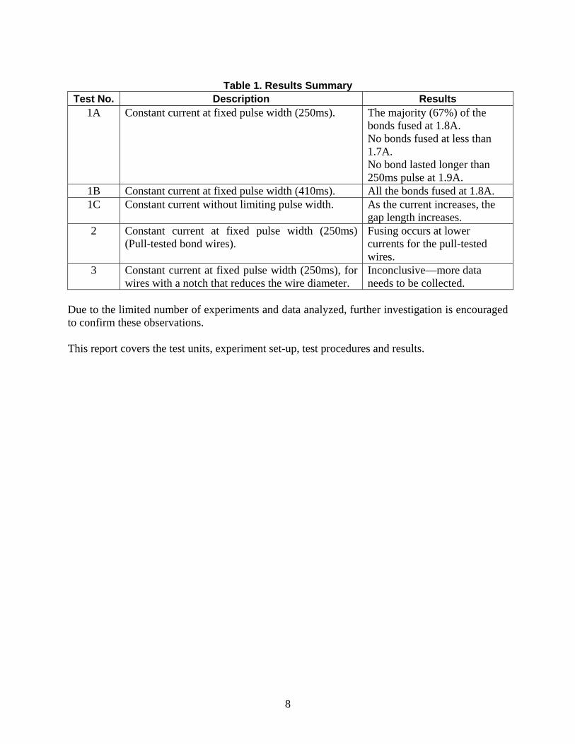
Table 1. Results Summary
Test No. Description Results 1A Constant current at fixed pulse width (250ms). The majority (67%) of the
bonds fused at 1.8A. No bonds fused at less than 1.7A. No bond lasted longer than 250ms pulse at 1.9A.
1B Constant current at fixed pulse width (410ms). All the bonds fused at 1.8A. 1C Constant current without limiting pulse width. As the current increases, the
gap length increases. 2 Constant current at fixed pulse width (250ms)
(Pull-tested bond wires). Fusing occurs at lower currents for the pull-tested wires.
3 Constant current at fixed pulse width (250ms), for wires with a notch that reduces the wire diameter.
Inconclusive—more data needs to be collected.
Due to the limited number of experiments and data analyzed, further investigation is encouraged to confirm these observations. This report covers the test units, experiment set-up, test procedures and results.

9
Intentionally Left Blank
10
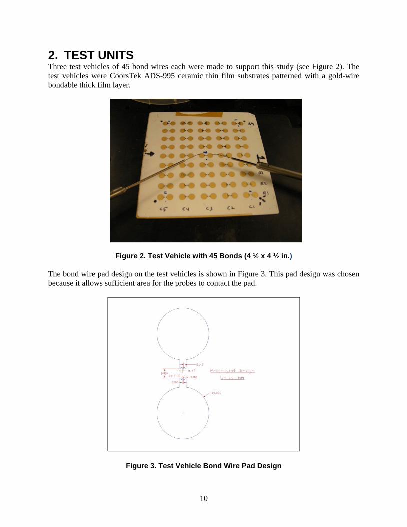
2. TEST UNITS Three test vehicles of 45 bond wires each were made to support this study (see Figure 2). The test vehicles were CoorsTek ADS-995 ceramic thin film substrates patterned with a gold-wire bondable thick film layer.
Figure 2. Test Vehicle with 45 Bonds (4 ½ x 4 ½ in.)
The bond wire pad design on the test vehicles is shown in Figure 3. This pad design was chosen because it allows sufficient area for the probes to contact the pad.
Figure 3. Test Vehicle Bond Wire Pad Design

11
Two images of a gold bond wire connected to the pads are shown in Figure 4. On the left side of Figure 4a is a “wedge” bond and on the right side a “ball” bond. The wires were bonded using an automatic wire bonder to ensure the length and quality of the bond wires would be as consistent as possible. In addition, each bond was inspected and measured prior to testing. See the appendices A-D for detailed information on the bond length and diameter for each test.
(a)
(b)
Figure 4. Scanning Electron Microscope (SEM) Image (a); Optical Image (b)

12
3. TEST EQUIPMENT CONFIGURATION Referring to Figure 5, the constant current test circuit uses a Hewlett Packard 6652A power supply (PS) to provide 6A of stable current to the bond wire (Rload). A stabilizer circuit provides a matching resistive load to the power supply before current is switched to Rload. This reduces current fluctuations and voltage spikes during the switching between the stabilizer and load circuits. Two power MOSFETs (IRL2203N), controlled by waveform generators (WG1 and WG2), provide synchronized switching of the power from the stabilizer circuit to the load circuit.
Figure 5. Constant Current Test Circuit
The calibration circuit enables initial testing of the constant current stability by switching between the stabilizer circuit and the calibration circuit. This allows tweaking of the capacitor (C1) and amplifier (LF353) gain (R1 and R2) to minimize voltage spikes. Final adjustments to stabilize signals were made by replacing the resistors (RS1 and RS2) with 0.1 ohm higher or lower values. The stabilized signals are confirmed by switching between the stabilizer circuit and load at 0.5A constant current. The waveform signals WG1, WG2, Vm1, and Vm2 were monitored with a Tektronix TDS 2024C oscilloscope. Figure 6 shows WG1 (yellow trace) switching off as WG2 switches on the MOSFET with a positive pulse to the gate. The current path changes from the stabilize circuit (as observed by the magenta trace) to the bond wire, Rload, shown by the green trace. Figure 6a shows the curve when the current is not sufficient to melt Rload. Figure 6b shows that the current stops flowing after 31ms (green trace).

13
31ms
(a) (b)
Figure 6. Green Trace Shows No Melting (a); Green Trace Shows Melting at 31ms (b) The thermal response of Rload was monitored using a Thermalyze Opthotherm EL (see Figure 7). A 9 x 5 matrix of 45 wires were placed under the thermal imaging camera and probed one at a time with micromanipulators (see Figure 8). The probes use a sharp 1.2 micron tungsten tip modified to provide more contact area and less contact resistance. The tip ends are bent slightly by overpressure on a gold pad, then with both probes on the same pad, high current (6A) is run through the probe tips to clean them. This reduces the total contact resistance from several ohms to less than 1 ohm. This also drops the required power supply voltage from above 12V to a manageable 3V at 2A. The thermal capture software allows video capture of the event and user defined areas to measure temperature on the images.
Figure 7. Test Set-up Switching Equipment on Left, Thermal Imaging Equipment on Right

14
Figure 8. Thermal Imaging of One Wire Bond on Test Vehicle with Current Provided by Probes
3.1. Length Calculations The gap length, as well as wire length and diameter, was measured by taking an image of a ruler (see Figure 9) and then taking an image of the bond wire at the same magnification. An image processing software package (ImageJ) uses the image of the ruler as a reference for distance (here, 1mm) and calculates the user’s desired length based on this reference. In this report, the yellow line on the figures is the user’s desired measurement.
Figure 9. Reference Measurement

15
Intentionally Left Blank

16
4. TEST PROCEDURES AND RESULTS 4.1. Test No. 1A: Constant Current at Fixed Pulse Width (250ms) The goal of this test was to determine the maximum current before the wire fused at a fixed pulse width of 250ms. If the wire did not fuse at 250ms, then the wire was allowed to cool to room temperature and then retested at a higher current. Figure 10 shows a fused bond wire. The data displayed in the image shows a gap length of 16.9 mil(0.43mm) at 4A.
Figure 10. Gap Length Measurement (16.9 mil)
4.1.1. Test Procedure Overview 1. SEM and optical image taken of each bond as a baseline. 2. Each bond tested, beginning at .5A and increased in .1A increments, limited to a 250ms
pulse width at each current until the bond wire fused. 3. Once the wire fused, data was recorded as shown in Appendix A. 4. Steps 1, 2, and 3 repeated for each bond wire.
4.1.2. Test Results 4.1.2.1. Summary A summary of the fusing currents is shown in Table 2. Following the table are images of a few of the results.
Table 2. Fusing Current Results Summary (250ms)
Number of Bonds (42 total)
Fusing Current (A)
1 1.7 28 1.8 13 1.9

17
The results are as follows: The majority (67%) of the bonds fused at 1.8A.
No bonds fused at less than 1.7A.
No bond lasted longer than the 250ms pulse at 1.9A.
Figure 11. 1.7A, Fused at 170s, Gap Length = 3.54 mil
Figure 12. 1.8A, Fused at 126s, Gap Length = 3.15 mil

18
Figure 13. 1.9A, Fused at 28s, Gap Length = 3.94 mil 4.1.2.2. Statistical Data Analysis The summary data in Table 2 and the raw data in Appendix A provide the basis for summary statistics, distribution estimates, and confidence statements regarding bond wire fusing times and currents for the levels tested. The next series of tests (1B, see Section 4.2) involves subjecting a different sample of bond wires to a similar series of tests using a 410ms pulse. A comparison of results from these two series of tests indicates that the results can be combined, which provide better estimates and confidence statements (see Appendix E). Consequently, a discussion of the combined results is provided in the next section. 4.1.2.3. Data Comparison to Theory In [Error! Bookmark not defined.], the fusing current is expressed in terms of a metal constant
M in the formula where A is in cm2 and L is in cm. For gold (Au), 4.68510 / . Given a bond wire length of 0.1524 cm and a reduction of 4.51 4.51 2.54 100.0115 , the fusing current is found to be
1.27 100.1409
4.685 10 1.7
which corresponds to the lowest fusing current measured.
19
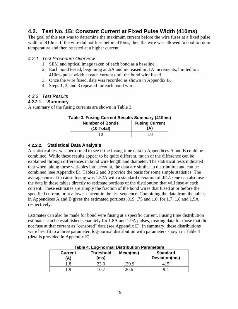
4.2. Test No. 1B: Constant Current at Fixed Pulse Width (410ms) The goal of this test was to determine the maximum current before the wire fuses at a fixed pulse width of 410ms. If the wire did not fuse before 410ms, then the wire was allowed to cool to room temperature and then retested at a higher current. 4.2.1. Test Procedure Overview
1. SEM and optical image taken of each bond as a baseline. 2. Each bond tested, beginning at .5A and increased in .1A increments, limited to a
410ms pulse width at each current until the bond wire fused. 3. Once the wire fused, data was recorded as shown in Appendix B. 4. Steps 1, 2, and 3 repeated for each bond wire.
4.2.2. Test Results 4.2.2.1. Summary A summary of the fusing currents are shown in Table 3.
Table 3. Fusing Current Results Summary (410ms) Number of Bonds
(10 Total) Fusing Current
(A)
10 1.8 4.2.2.2. Statistical Data Analysis A statistical test was performed to see if the fusing time data in Appendices A and B could be combined. While these results appear to be quite different, much of the difference can be explained through differences in bond wire length and diameter. The statistical tests indicated that when taking these variables into account, the data are similar in distribution and can be combined (see Appendix E). Tables 2 and 3 provide the basis for some simple statistics. The average current to cause fusing was 1.82A with a standard deviation of .047. One can also use the data in these tables directly to estimate portions of the distribution that will fuse at each current. These estimates are simply the fraction of the bond wires that fused at or before the specified current, or at a lower current in the test sequence. Combining the data from the tables in Appendices A and B gives the estimated portions .019, .75 and 1.0, for 1.7, 1.8 and 1.9A respectively. Estimates can also be made for bond wire fusing at a specific current. Fusing time distribution estimates can be established separately for 1.8A and 1.9A pulses, treating data for those that did not fuse at that current as "censored" data (see Appendix E). In summary, these distributions were best fit to a three parameter, log-normal distribution with parameters shown in Table 4 (details provided in Appendix E).
Table 4. Log-normal Distribution Parameters Current
(A) Threshold
(ms) Mean(ms) Standard
Deviation(ms)
1.8 23.0 139.9 415 1.9 10.7 20.6 9.4

20
Stronger statistical statements are possible that reflect the limitations in the number and type of data and provide confidence statements associated with the inferences. The results are summarized below and more detail on the analysis is provided in Appendix F. Consider the statements:
(*) YY% certainty that at least XX% of the bond wire population will yield a fusing response lower than Tu; or
(**) YY% certainty that at least XX% of the bond wire population will yield a fusing response higher than Tl.
The percentages YY and XX and the thresholds Tu and Tl are parameters of the statement. These statements are based on statistical tolerance bounds, defined as confidence bounds on distribution percentiles. Statements (*) and (**) can be used to estimate the bond wire performance as a function of time for any given current where at least two test units fused. The estimates and bounds in the table below address the question: “How long will it take for the bond wire to fuse when subjected to the current given in the first column?” The table below provides tolerance bounds based on this data. Similar tables can be produced for other values of XX and YY.
Table 5. Tolerance Bounds
Current (A)
YY (%)
XX=.5 (lower bound)
(ms)
XX=.95 (upper bound)
(ms)
Estimate (lower bound)
(ms)
Estimate (upper bound)
(ms) 1.8 90 24.3 789.6 25.3 472.5 1.9 90 11.8 58.5 12.5 37.6
As an example of how one might use these tables, the statement can be made that with 90% certainty, 95% of the bond wires will fuse at or before 58.5ms when exposed to a 1.9A pulse. The expected time of fusing at this current is 20.6ms (from Table 4). It is important to note that some of the variability contributing to the standard deviation and fairly wide tolerance bounds is the result of differences in the bond wire length and diameter (both have a significant effect on fusing time). 4.3. Test No. 1C: Constant Current (2A – 6A) The goal of this test was to determine the impact of current on the gap length of the bond wire after fusing. The pulse width was not limited as in Test No. 1A and1B. The bond wires were subjected to a constant current until they fused.

21
4.3.1. Test Procedure 1. SEM and optical image taken of each bond as a baseline. 2. Each bond tested beginning at 2A and increasing in 2A increments up to 6A,
unlimited pulse length. 3. Once the wire fused, data was recorded as shown in Appendix C. 4. Steps 1, 2, and 3 repeated for each bond wire.
4.3.2. Test Results 4.3.2.1. Summary The fusing current data is summarized in Figure 14. The results show that in general, the gap length increases as the current increases.
Figure 14. Current vs. Gap Length
Figure 15. 2A, Fused at 9.4ms, GAP Length = 5.31 mil
0
0.1
0.2
0.3
0.4
0.5
0.6
0.7
0.8
0.9
1
0 1 2 3 4 5 6 7
Gap
Length (mm)
Current (A)
Current vs Gap Length
Bond Wire
22
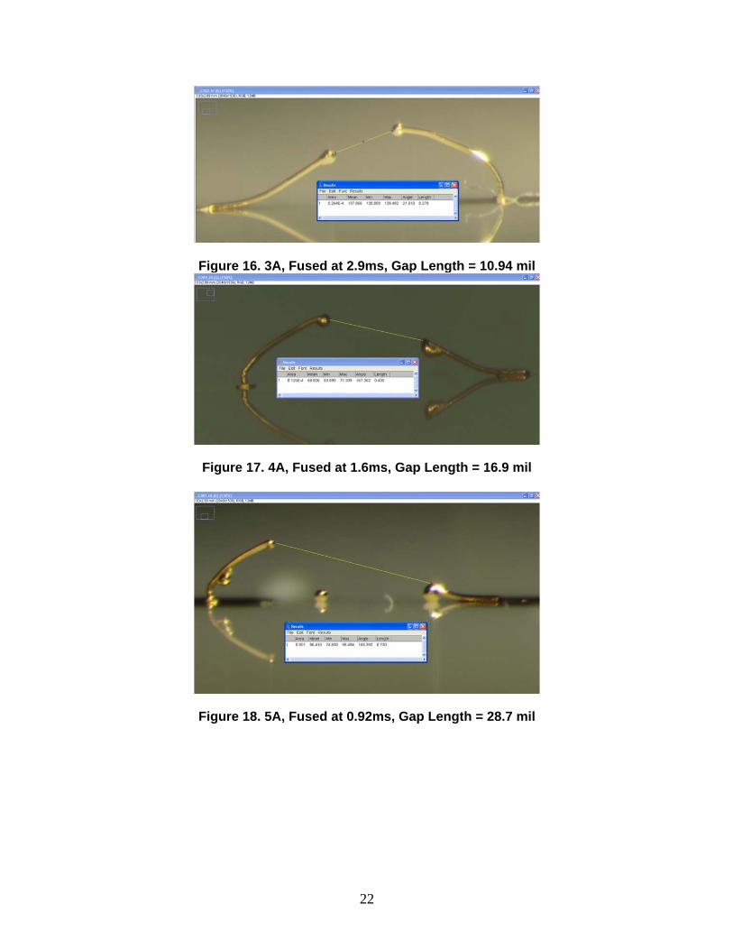
Figure 16. 3A, Fused at 2.9ms, Gap Length = 10.94 mil
Figure 17. 4A, Fused at 1.6ms, Gap Length = 16.9 mil
Figure 18. 5A, Fused at 0.92ms, Gap Length = 28.7 mil
23
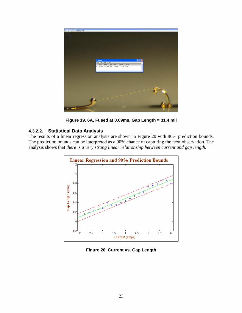
Figure 19. 6A, Fused at 0.69ms, Gap Length = 31.4 mil 4.3.2.2. Statistical Data Analysis The results of a linear regression analysis are shown in Figure 20 with 90% prediction bounds. The prediction bounds can be interpreted as a 90% chance of capturing the next observation. The analysis shows that there is a very strong linear relationship between current and gap length.
Figure 20. Current vs. Gap Length
24
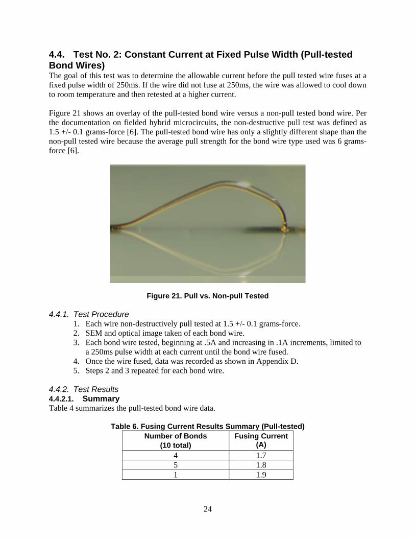
4.4. Test No. 2: Constant Current at Fixed Pulse Width (Pull-tested Bond Wires) The goal of this test was to determine the allowable current before the pull tested wire fuses at a fixed pulse width of 250ms. If the wire did not fuse at 250ms, the wire was allowed to cool down to room temperature and then retested at a higher current. Figure 21 shows an overlay of the pull-tested bond wire versus a non-pull tested bond wire. Per the documentation on fielded hybrid microcircuits, the non-destructive pull test was defined as 1.5 +/- 0.1 grams-force [6]. The pull-tested bond wire has only a slightly different shape than the non-pull tested wire because the average pull strength for the bond wire type used was 6 grams-force [6].
Figure 21. Pull vs. Non-pull Tested 4.4.1. Test Procedure
1. Each wire non-destructively pull tested at 1.5 +/- 0.1 grams-force. 2. SEM and optical image taken of each bond wire. 3. Each bond wire tested, beginning at .5A and increasing in .1A increments, limited to
a 250ms pulse width at each current until the bond wire fused. 4. Once the wire fused, data was recorded as shown in Appendix D. 5. Steps 2 and 3 repeated for each bond wire.
4.4.2. Test Results 4.4.2.1. Summary Table 4 summarizes the pull-tested bond wire data.
Table 6. Fusing Current Results Summary (Pull-tested) Number of Bonds
(10 total) Fusing Current
(A)
4 1.7 5 1.8 1 1.9
25
4.4.2.2. Statistical Data Analysis Statistical tests indicate significant differences between the pull-tested bond wires and those in the other two samples in Test No. 1A and 1B (listed in Appendices A and B). The summary in Table 4 shows that in general, fusing occurred for the pull-tested wires at lower currents. Because of the limited number of data, it is not possible to get a good estimate of fusing-time distribution. A rough estimate for 1.8A is provided in Table 7, based on a three parameter, log-normal distribution. See Appendix E for details on the statistical testing.
Table 7. Estimate for Distribution of Fusing Times Current
(A) Threshold(ms) Mean(ms) Standard
Deviation(ms)
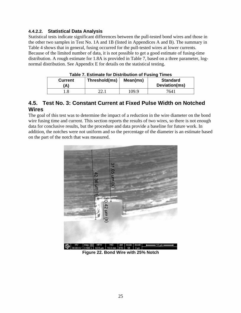
1.8 22.1 109.9 7641 4.5. Test No. 3: Constant Current at Fixed Pulse Width on Notched Wires The goal of this test was to determine the impact of a reduction in the wire diameter on the bond wire fusing time and current. This section reports the results of two wires, so there is not enough data for conclusive results, but the procedure and data provide a baseline for future work. In addition, the notches were not uniform and so the percentage of the diameter is an estimate based on the part of the notch that was measured.
Figure 22. Bond Wire with 25% Notch
26
4.5.1. Test Procedure 1. SEM and optical image taken of each bond wire. 2. Each bond wire tested, beginning at .5A and increased in .1A increments, limited to a
250ms pulse width at each current until the bond wire fused. 3. Once the wire fused, data was recorded as shown in the summary section below. 4. Steps 2 and 3 repeated for each bond wire.
4.5.2. Test Results 4.5.2.1. Summary Table 8 summarizes the notched bond wire data.
Table 8. Fusing Current with Notched Wires Results Summary Diameter
Reduction (%)
Number of Bonds (2 total)
Fusing Current (A)
Fusing Time (ms)
25 1 1.8 35.4 27 1 1.8 41.6
4.5.2.2. Statistical Data Analysis No meaningful data analysis could be done due to the small sample size. Section 5.2 describes proposed future work.

27
Intentionally Left Blank

28
5. CONCLUSIONS 5.1. Key Results Based on the data obtained to date, the conclusions are as follows:
Majority (73%) of the bonds fused at 1.8A (for samples that were not pull tested)
No bonds fused at less than 1.7A (lower bound)
No bond lasted longer than 60ms at 1.9A (upper bound)
As current increases, the gap length increases (approximately linearly)
5.2. Future Work Table 9 details the future work that could be performed for each of the characterization tests described in this report.
Table 9. Future Work Summary Test No. Description Future Work
1A Constant current at fixed pulse width (250ms). Test additional bond wires. 1B Constant current at fixed pulse width (410ms). Test additional bond wires. 1C Constant current without limiting pulse width. Test additional bond wires and
vary the current to lower than 2A and higher than 6A.
2 Constant current at fixed pulse width (250ms), for pull-tested bond wires.
Test additional bond wires.
3 Constant current at fixed pulse width (250ms), for notched wires that reduce the wire diameter.
Test additional bond wires and perform analysis comparing these results to the Test 1A, 1B, 1C and 2 results.

29
Intentionally Left Blank

30
6. REFERENCES 1. Chen, Kenneth C. and Brigham, William P., “EBW Gapping Study,” SAND2001-0698, Sandia National Laboratories, Albuquerque, NM, March 2001. 2. Chen, Kenneth C., Tom (T) Y. Lin and Larry K. Warne, “Bond Wire and Bridge-wire Fusing,” SAND2011-1658, Sandia National Laboratories, Albuquerque, NM, March 2011. 3. Krabbenborg, B., “High current bond design rules based on bond pad degradation and fusing of the wire,” Microelectronics Reliability, vol. 39, no. 1, pp. 77-88, 1999. 4. Loh, Eugene, “Physical Analyses for Data on Fused-Open Bond Wires,” IEEE Transactions on Components, Hybrids, and Manufacturing Technology, vol.6, no.2, pp. 209-217, 1983. 5. Mertol, Atila, “Estimation of Aluminum and Gold Bond Wire Fusing Current and Fusing Time,” IEEE Transactions on Components, Hybrids, and Manufacturing Technology, vol.18, no.1, pp. 210-214, 1995. 6. Peck, D., “Gold Fine Wire Bonding,” SS289361, Sandia National Laboratories, September 1994. 7. Strutt, J.W., Lord Rayleigh, “On the Instability of Cylindrical Fluid Surfaces,” Philosophical Magazine, vol. 34, pp. 177-180, 1892.

31
Intentionally Left Blank

32
APPENDIX A – TEST NO. 1A DATA Note: Bond No. 1, 2 and 4 were not tested.
Bond Wire No.
Diameter (um)
Length (mm)
Fusing Time (ms)
Fusing Current
(A)
Gap Length After
Melting (mm)
1 27.98 1.51 1.8 0.09 2 26.66 1.51 1.8 0.09 3 27.97 1.40 28 1.9 0.10 4 27.39 1.41 0.09 5 26.81 1.42 52 1.9 0.08 6 26.23 1.41 58.8 1.9 0.08 7 25.64 1.46 196 1.8 0.09 8 26.42 1.51 30 1.8 0.10 9 25.84 1.51 29 1.8 0.10 10 27.39 1.54 29.6 1.8 0.09 11 27.59 1.53 70 1.8 0.08 12 27.78 1.50 45 1.8 0.09 13 27.59 1.51 36 1.8 0.09 14 27.00 1.52 24 1.9 0.09 15 27.59 1.46 31 1.9 0.09 16 27.39 1.47 126 1.8 0.08 17 27.39 1.51 32 1.8 0.09 18 27.78 1.50 23 1.9 0.09 19 27.39 1.52 24 1.8 0.10 20 27.00 1.53 28 1.8 0.10 21 27.59 1.51 46 1.8 0.09 22 27.78 1.50 74 1.8 0.09 23 27.98 1.53 38 1.8 0.10 24 26.62 1.49 184 1.8 0.09
25 27.20 1.51 34 1.8 0.10 26 27.59 1.52 37 1.8 0.09 27 27.39 1.51 38 1.8 0.09 28 27.59 1.52 33 1.8 0.10 29 27.20 1.53 50 1.8 0.09 30 28.36 1.51 73 1.8 0.08 31 27.2 1.40 42 1.8 0.09 32 27.2 1.53 43 1.8 0.09 33 27.59 1.49 170 1.7 0.09 34 27.00 1.43 36 1.9 0.09

33
Bond Wire No.
Diameter (um)
Length (mm)
Fusing Time (ms)
Fusing Current
(A)
Gap Length After
Melting (mm)
35 27.78 1.50 218 1.8 0.09 36 27.39 1.49 76 1.8 0.09 37 28.36 1.52 24 1.9 0.09 38 27.78 1.51 54 1.8 0.08 39 28.36 1.50 27 1.9 0.09 40 29.14 1.46 31 1.9 0.09 41 29.14 1.50 30 1.9 0.09 42 27.00 1.48 36 1.9 0.08 43 27.59 1.52 33 1.9 0.09 44 27.39 1.52 54 1.8 0.08 45 28.17 1.52 46 1.8 0.09

34
APPENDIX B – TEST NO. 1B DATA
Bond Wire No.
Diameter (um)
Length (mm)
Fusing Time (ms)
Fusing Current
(A)
Gap Length After
Melting (mm)
1 26.81 1.538 56.59 1.8 0.094 2 27.10 1.584 29.99 1.8 0.097 3 26.81 1.544 36.00 1.8 0.095 4 26.52 1.521 30.39 1.8 0.103 5 25.21 1.527 31.19 1.8 0.102 6 25.79 1.553 32.39 1.8 0.099 7 26.08 1.529 35.79 1.8 0.097 8 25.94 1.559 30.19 1.8 0.096 9 26.52 1.583 28.78 1.8 0.097 10 27.25 1.558 52.60 1.8 0.090
35
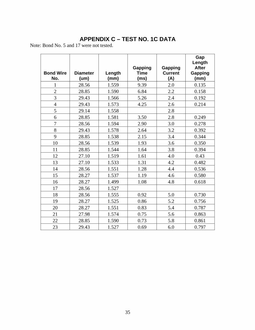
APPENDIX C – TEST NO. 1C DATA
Note: Bond No. 5 and 17 were not tested.
Bond Wire No.
Diameter (um)
Length (mm)
Gapping Time (ms)
Gapping Current
(A)
Gap Length After
Gapping (mm)
1 28.56 1.559 9.39 2.0 0.135 2 28.85 1.590 6.84 2.2 0.158 3 29.43 1.566 5.26 2.4 0.192 4 29.43 1.573 4.25 2.6 0.214 5 29.14 1.558 2.8 6 28.85 1.581 3.50 2.8 0.249 7 28.56 1.594 2.90 3.0 0.278 8 29.43 1.578 2.64 3.2 0.392 9 28.85 1.538 2.15 3.4 0.344 10 28.56 1.539 1.93 3.6 0.350 11 28.85 1.544 1.64 3.8 0.394 12 27.10 1.519 1.61 4.0 0.43 13 27.10 1.533 1.31 4.2 0.482 14 28.56 1.551 1.28 4.4 0.536 15 28.27 1.537 1.19 4.6 0.580 16 28.27 1.499 1.08 4.8 0.618 17 28.56 1.527 18 28.56 1.555 0.92 5.0 0.730 19 28.27 1.525 0.86 5.2 0.756 20 28.27 1.551 0.83 5.4 0.787 21 27.98 1.574 0.75 5.6 0.863 22 28.85 1.590 0.73 5.8 0.861 23 29.43 1.527 0.69 6.0 0.797
36
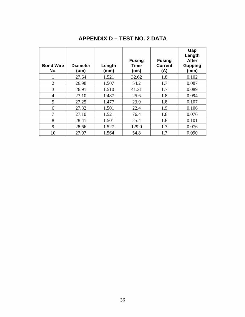
APPENDIX D – TEST NO. 2 DATA
Bond Wire No.
Diameter (um)
Length (mm)
Fusing Time (ms)
Fusing Current
(A)
Gap Length After
Gapping (mm)
1 27.64 1.521 32.62 1.8 0.102 2 26.98 1.507 54.2 1.7 0.087 3 26.91 1.510 41.21 1.7 0.089 4 27.10 1.487 25.6 1.8 0.094 5 27.25 1.477 23.0 1.8 0.107 6 27.32 1.501 22.4 1.9 0.106 7 27.10 1.521 76.4 1.8 0.076 8 28.41 1.501 25.4 1.8 0.101 9 28.66 1.527 129.0 1.7 0.076 10 27.97 1.564 54.8 1.7 0.090

37
APPENDIX E – STATISTICAL TESTING
Statistical tests were performed to compare data acquired from the 250ms and 410ms pulse tests. These data are described in Sections 4.1 and 4.2 and are given in Appendicies A and B. Because all the responses from testing using 410ms pulses resulted in fusing at 1.8A, the only comparison made was at this current. For this comparison, one observation was considered to be “left-censored” (one only knows that it had fused by time t) and a number of observations were considered to be “right-censored” (one only knows that they had not fused at time 250ms). The censored observations, together with the set of bond wires that failed at 1.8A, provide the basis for the 250ms test results. The bond wire that fused at 1.7A was treated using the following assumptions:
1) A bond wire that fused at a lower current would fuse at the higher testing current in less or equal time; and
2) A bond wire that fused at a lower current would fuse at the higher testing current before any of the bond wires that did not fuse at the lower current.
Note that assumption 1) does not require an understanding about the relationship between testing at the different currents, beyond assuming the higher current will cause fusing at least as fast as the lower current. Assumption 2) carries the assumption that not fusing at a lower current indicates a “stronger” bond wire, and hence at the higher current the bond wires that did fuse at the lower current would fuse earlier. This assumption seems reasonable if, for example, the fusing is strictly a function of the temperature achieved by the bond wire during testing. Statistical tests for the censored data were performed using Minitab® software. The following shows the resulting ANOVA table. Column “P” shows the p-values related to the testing. Using p = .05 (or most any reasonable value) as a significance level, the table indicates that bond length and diameter are significant in determining fusing time, however “test set” is not. Test set is being used as an indicator variable to distinguish between the 250ms and 410ms pulse results. As a result of these tests the two data sets were combined.

38
Response Variable Start: start 1.8 End: alt end 1.8 Censoring Information Count Uncensored value 38 Right censored value 13 Left censored value 1 Estimation Method: Maximum Likelihood Distribution: Weibull Regression Table
Standard 95.0% Normal CI
Predictor Coef Error Z P Lower Upper
Intercept 25.1531 8.5637 2.94 0.003 8.36854 41.9376
test set 1 -0.33138 0.513171 -
0.65 0.518 -1.33718 0.674418
Bond Length -22.9201 5.80033 -
3.95 0 -34.2885 -11.5517
Diameter 0.530564 0.200275 2.65 0.008 0.138031 0.923096
Shape 1.24202 0.157431 0.968803 1.59229 Log-Likelihood = -210.046
Similar statistical tests were performed to compare the combined data discussed above and the pull-tested bond wire data described in Section 4.4. In the ANOVA table below, “test set” is used to distinguish between the combined results and the pull tested responses. In this case, the p-value .026 indicates a significant difference. Response Variable Start: start 1.8 End: alt end 1.8 Censoring Information Count Uncensored value 43 Right censored value 14 Left censored value 5 Estimation Method: Maximum Likelihood Distribution: Weibull

39
Regression Table
Standard 95.0% Normal CI
Predictor Coef Error Z P Lower Upper
Intercept 25.8207 8.61024 3.00 0.003 8.94493 42.6964
test set_1 1 0.787882 0.353983 2.23 0.026 0.0940884 1.48168
Bond Length 21.5984 4.23421 -
5.10 0.000 -29.8973 -13.2995
Diameter 0.393815 0.176404 2.23 0.026 0.0479993 0.739631
Shape 1.09117 0.129746 0.86433 1.37754 Log-Likelihood = -243.393

40
Intentionally Left Blank
41
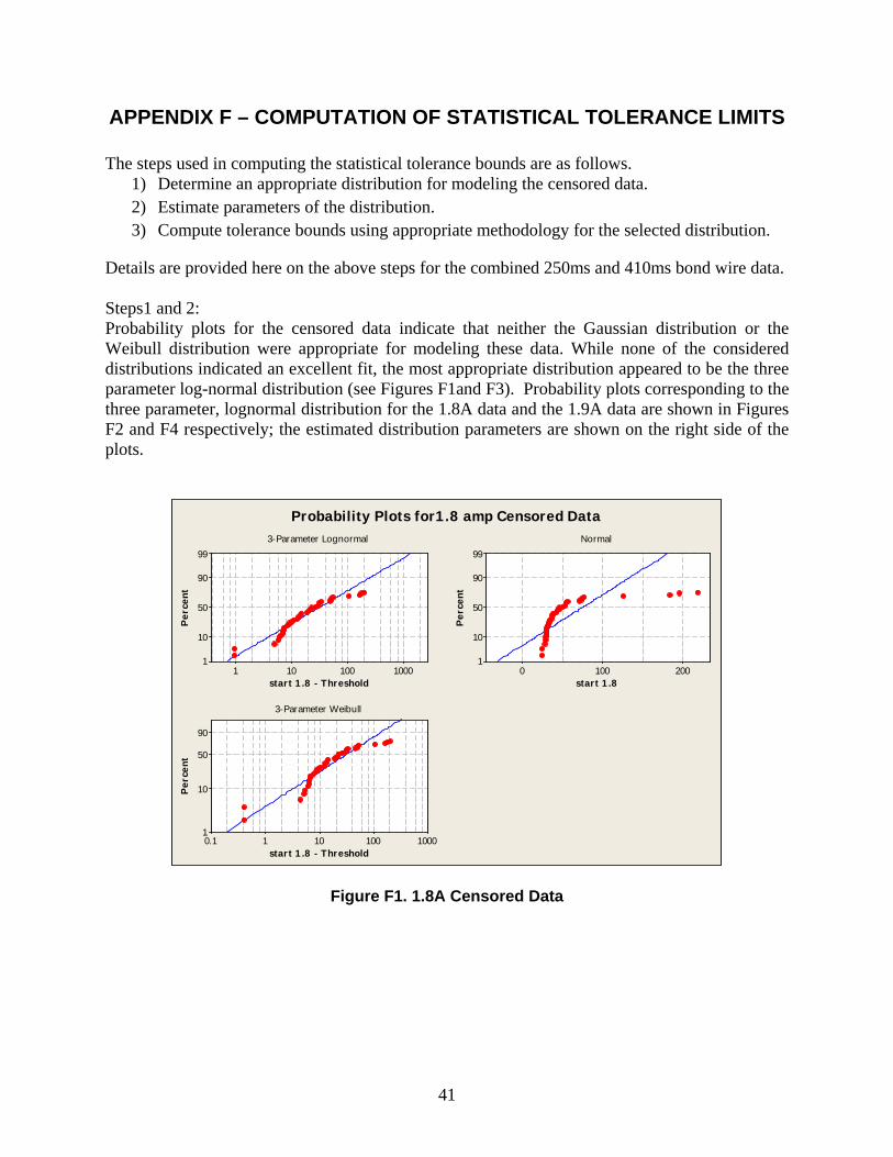
APPENDIX F – COMPUTATION OF STATISTICAL TOLERANCE LIMITS
The steps used in computing the statistical tolerance bounds are as follows. 1) Determine an appropriate distribution for modeling the censored data. 2) Estimate parameters of the distribution. 3) Compute tolerance bounds using appropriate methodology for the selected distribution.
Details are provided here on the above steps for the combined 250ms and 410ms bond wire data. Steps1 and 2: Probability plots for the censored data indicate that neither the Gaussian distribution or the Weibull distribution were appropriate for modeling these data. While none of the considered distributions indicated an excellent fit, the most appropriate distribution appeared to be the three parameter log-normal distribution (see Figures F1and F3). Probability plots corresponding to the three parameter, lognormal distribution for the 1.8A data and the 1.9A data are shown in Figures F2 and F4 respectively; the estimated distribution parameters are shown on the right side of the plots.
1000100101
99
90
50
10
1
start 1.8 - Threshold
Per
cent
2001000
99
90
50
10
1
start 1.8
Per
cent
10001001010.1
90
50
10
1
start 1.8 - Threshold
Per
cent
Probability Plots for1.8 amp Censored Data3-Parameter Lognormal Normal
3-Parameter Weibull
Figure F1. 1.8A Censored Data

42
100001000100101
99
95
90
80
7060504030
20
10
5
1
start 1.8 - Threshold
Perc
ent
Loc 3.45493Scale 1.61604Thres 23.0416Mean 139.871StDev 415.041Median 54.6975IQ R 83.5103A D* 54.893C orrelation 0.957
Table of Statistics
Probability Plot fo 1.8 amp Data
Arbitrary Censoring3-Parameter Lognormal - 80% CI
Figure F2. 1.8A Data
100101
99
90
50
10
1
start 1.9 - Threshold
Per
cent
40200-20
99
90
50
10
1
start 1.9
Per
cent
1001010.10.01
90
50
10
1
start 1.9 - Threshold
Per
cent
Probability Plots for1.9 amp Censored Data3-Parameter Lognormal Normal
3-Parameter Weibull
Figure F3. 1.9A Censored Data

43
70605040302015
99
95
90
80
7060504030
20
10
5
1
start 1.9 - Threshold
Perc
ent
Loc 1.97502Scale 0.800627Thres 10.6744Mean 20.6040StDev 9.41162Median 17.8811IQ R 8.16738A D* 6.416C orrelation 0.975
Table of Statistics
Probability Plot fo 1.9 amp Data
Arbitrary Censoring3-Parameter Lognormal - 80% CI
Figure F4. 1.9A Data Step 3: An appropriate way to compute tolerance bounds for these data is to transform the data to the Gaussian distribution by subtracting the threshold and taking the logarithm. Tolerance bounds are then computed using standard Gaussian methods (i.e., using the non-central t-distribution); the reverse transformation is then used to obtain the appropriate bounds. This process was applied here and the results provided in Section 4.2.

44
Intentionally Left Blank
45
DISTRIBUTION 4 Lawrence Livermore National Laboratory Attn: N. Dunipace (1) P.O. Box 808, MS L-795
Livermore, CA 94551-0808 1 MS0447 Michael F. Hall 2111 1 MS0492 Kenneth C. Chen 0411 1 MS0634 Van T. Pham 2958 1 MS0665 James A. Woods II 2542 1 MS0959 Brian Wroblewski 1833 1 MS9014 Dawn M. Skala 8238 1 MS9014 Robert L. Kinzel 8238 1 MS9154 Stephan L. King-Monroe 8237 1 MS0899 Technical Library 9536 (electronic copy)

46
