1

Mining Quantitative Association Rules Mining Quantitative Association Rules in Large Relational Databasein Large Relational Database

Presented by Jin Jin

April 1, 2004

2

ReviewReview

Association Rules –interesting association relationship among huge amounts of transactionsAn association rule is an expression of the form X => Y, where X and Y are sets of itemsGoal of AA – To find all association rules that satisfy user-specified minimum support and minimum confidence threshold

3

OutlineOutline

• Introduction• 5 steps of discovering quantitative

association rules• Partitioning quantitative attributes• Interest • Algorithm• Conclusion

4

IntroductionIntroduction

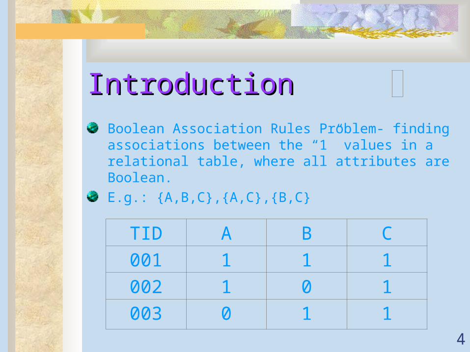
Boolean Association Rules Problem- finding associations between the “1” values in a relational table, where all attributes are Boolean.

E.g.: {A,B,C},{A,C},{B,C}

TID A B C

001 1 1 1

002 1 0 1

003 0 1 1

5

Introduction,CONTIntroduction,CONT

Most Databases have Richer Attributes types

e.g. Quantitative: Age, Income

Categorical: Zip, Make of Car

Quantitative Association Rules Problems - Mining association rules over quantitative and categorical attributes

6

Mapping Quantitative Association Rules Mapping Quantitative Association Rules Problem into the Boolean Association Problem into the Boolean Association Rules ProblemRules Problem

If all attributes are categorical or the quantitative attributes have only a few values, we could map each<attribute, value> pair to a boolean attribute.

If the domain of values for a quantitative attribute is large, first partition the values into intervals and then map each <attribute, interval> pair to a boolean attribute.

7

RecID Age: 20..2

5

Age: 26..35

Married: Yes

Married: No

NumCars: 0

NumCars: 1

100 1 0 0 1 0 1

200 1 0 1 0 0 1

300 0 1 1 0 1 0

400 0 1 0 1 1 0

RecordID Age Married NumCars

100 23 No 1

200 25 Yes 1

300 29 Yes 0

300 33 No 0

8

Mapping ProblemsMapping Problems

MinSup – If the number of intervals for a quantitative attribute is large, the support for any single interval can be low

MinConf – Information lost due to partitioning into intervals. This information lost increases as the interval sizes become larger.

9

Catch-22Catch-22

If intervals are too large, rules may not have MinConf

If intervals are too small, rules may not have MinSup

How do we solve it ?

10

Solve Catch-22Solve Catch-22

Consider all possible continuous ranges over the values of the quantitative attribute, or over the partitioned intervals

Solve minimum support – combine adjacent intervals/values

Solve minimum confidence – increase number of intervals

11

Unfortunately , More ProblemsUnfortunately , More ProblemsExec Time – If a quantitative attribute has n values(or intervals), there are on average O(n2) ranges that include a specific value or interval.

Many Rules – If a value(or interval) has MinSup, then any range containing this value also has MinSup, thus producing many uninteresting rules.

12

Our ApproachOur Approach

Maximum Support – stop combining adjacent intervals if their combined support exceeds this value

Partial Completeness – quantify information lost due to partitioning

Interest Measure – help prune out uninteresting rules

13

Problem definitionProblem definition

The rule X=>Y holds in the record set D with confidence c if c% of records in D that support X also support Y.

The rule X=>Y has support s in the record set D if s% of records in D support XUY

14

Formal Problem StatementFormal Problem Statement

“ Given a set of Records D, the problem of mining quantitative association rules is to find all quantitative association rules that have support and confidence greater than the user-specified minimum support and minimum confidence”

15

5 steps of discovering quantitative 5 steps of discovering quantitative association rulesassociation rules

1) Determine the number of partitions for each quantitative attribute

2) Mapping the values of each attribute to a set of consecutive integers, such that the order of the values is preserved

3) Find the support for each value of both quantitative and categorical attributes. For quantitative attributes, adjacent values are combined as long as their support is less than the user-specified maximum support. Next,generate the frequent itemsets.

4) Use Frequent itemsets to generate association rules5) Determining the interesting rules.

16

17

Partitioning Quantitative attributesPartitioning Quantitative attributes

Partial Completeness – Gives a handle on the amount of information lost by partitioning. The lower the level of partial completeness, the less the information lost.

Equi-Depth Partitioning – Minimizes the number of intervals required to satisfy Partial Completeness level

18

Partial CompletenessPartial Completeness

R – Set of rules generated by considering all ranges over the raw values

R’ – Set of rules generated by considering all ranges over the partitions

Measure the information loss – for each rule in R, how “far” the “closest” rule in R’ is

Using the ratio of the support of the rules as a measure of how far apart the rules are

19

Partial Completeness Over ItemsetsPartial Completeness Over ItemsetsLet C denote the set of all frequent itemsets in D. For any , we call P K-complete w.r.t C if

1KCP

PXXXPX '' and

)(support*)support( and Y

oftion generaliza a is Ysuch that Y )

)(support*)support(

and X oftion generaliza a is i)

such that

'

'''

'

'

'

YKY

XXYii

XKX

X

PXCX

20

Sample Partial CompletenessSample Partial CompletenessNumber Itemset Support

1 Age: 20-30 5%

2 Age: 20-40 6%

3 Age: 20-50 8%

4 Cars: 1-2 5%

5 Cars: 1-3 6%

6 Age: 20-30, Cars 1-2 4%

7 Age: 20-40, Cars 1-3 5%

Itemsets 2,3,5,7 form a 1.5-complete set

21

Close RuleClose Rule

Given a set of frequent itemsets P which is K-complete w.r.t. the set of all frequent itemsets, the minimum confidence when generating rules from P must be set to 1/K times the desired level to guarantee that a close rule will be generated

22

Determining Number of PartitionsDetermining Number of Partitions

Given A Partial Completeness Level K, and Equi-Depth partitioning, we get

Number of Intervals = where n = Number of quantitative attributes m = Minimum support K = Partial Completeness Level

)1(

2

km

n

23

InterestInterest

Consider the following rules, where about a quarter of people in the age group 20..30 are in the age group 20..25

Age: 20-30 =>Cars: 1..2 (8% Supp, 70% Conf)

Age: 20-25 =>Cars: 1..2 (2% Supp, 70% Conf)

Second Rule Redundant

Capture Rules by “Greater than Expected”

24

Expected ValuesExpected Values

Epr(Z’)[Pr(Z)] – the “expected” value of Pr(Z) based on Pr(Z’), where Z’ is a generalization of Z

Epr(Y’|X’)[Pr(Y|X)] – the “expected” confidence of the rule X=>Y based on the rule X’=>Y’, where X’ and Y’ are generalizations of X and Y, respectively.

25

Expected Values, ContExpected Values, Cont

26

Interest MeasureInterest Measure

A Rule X =>Y is R-Interesting w.r.t X’ => Y’ if the support of the rule X=>Y is R times the expected support based on X’ => Y’,

Or the confidence is R times the expected confidence based on X’ => Y’ , and the itemset X U Y is R-interesting w.r.t X’ U Y’.

27

Algorithm—finding frequent itemsetAlgorithm—finding frequent itemset

Based on the Apriori algorithm for finding boolean association rules

Candidate Generation

Join Phase

Subset Prune Phase

Interest Prune Phase

Counting Support of Candidates

28

Algorithm’ContAlgorithm’Cont

K-itemset denote an itemset having k-items

L k : Set of Frequent k - itemsets

L k –1 is used to generate C k , the Candidate k-Itemsets

Scan Database, determine which of the candidates in C k are contained in the record, and their support increment by one

At the end of the pass, C k is examined and yield L k.

29

Candidate GenerationCandidate Generation

Join Phase: L k-1 is joined with itself, first k-2 items are the same, and the attributes of the last two items are different.

e.g. L2{<Married: Yes><Age 20..24>}{<Married: Yes><Age 20..29>}{<Married: Yes> <NumCars: 0..1>}{<Age:20..29><NumCars: 0..1>}

After the Join step, C3 will consist of the following:{<Married: Yes><Age 20..24> <NumCars: 0..1>}{<Married: Yes><Age 20..29><NumCars: 0..1>}

30

Candidate GenerationCandidate GenerationSubset Prune Phrase:Join Results having some (k-1)-subset that is not in L k-1 are deleted

Delete: (Married: yes; Age 20..24; NumCars: 0..1)

(Age: 20..24; NumCars: 0..1) Not in L2

Interest Prune Phase: Further pruning candidate set according to user-specified interest level

31

Counting Support of CandidatesCounting Support of CandidatesPartition candidates into groups such that candidates in each group have the same attributes and the same values for categorical attributes.

Replace each group with a single super candidate. 1) The common categorical attribute values 2) A data structure representing the set of values of the quantitative attributes e.g. {<Married: Yes><Age 20..24> <NumCars: 0..1>}

{<Married: Yes><Age 20..29><NumCars: 1..2>}

32

Counting Support of Candidates’ContCounting Support of Candidates’Cont

Find which “super-candidates” are supported by the categorical attributes in the record.

If categorical attributes of a “super-candidates” are supported by a given record, we need to find which of the candidates in the super-candidates are supported by quantitative attributes.

33

ConclusionConclusion

Partitioning and combining adjacent partitions

Partial Completeness

“Greater-than-expected-value” interest measure

34

Questions??Questions??