1

Norm-Preservation: Why Residual NetworksCan Become Extremely Deep?

Alireza Zaeemzadeh, Student Member, IEEE, Nazanin Rahnavard, Senior Member, IEEE,and Mubarak Shah, Fellow, IEEE

Abstract—Augmenting neural networks with skip connections, as introduced in the so-called ResNet architecture, surprised thecommunity by enabling the training of networks of more than 1,000 layers with significant performance gains. This paper deciphersResNet by analyzing the effect of skip connections, and puts forward new theoretical results on the advantages of identity skipconnections in neural networks. We prove that the skip connections in the residual blocks facilitate preserving the norm of the gradient,and lead to stable back-propagation, which is desirable from optimization perspective. We also show that, perhaps surprisingly, as moreresidual blocks are stacked, the norm-preservation of the network is enhanced. Our theoretical arguments are supported by extensiveempirical evidence.Can we push for extra norm-preservation? We answer this question by proposing an efficient method to regularize the singular values ofthe convolution operator and making the ResNet’s transition layers extra norm-preserving. Our numerical investigations demonstrate thatthe learning dynamics and the classification performance of ResNet can be improved by making it even more norm preserving. Ourresults and the introduced modification for ResNet, referred to as Procrustes ResNets, can be used as a guide for training deepernetworks and can also inspire new deeper architectures.

Index Terms—Residual Networks, Convolutional Neural Networks, Optimization Stability, Norm Preservation, Spectral Regularization.

F

1 INTRODUCTION

Deep neural networks have progressed rapidly during thelast few years, achieving outstanding, sometimes superhuman, performance [1]. It is known that the depth ofthe network, i.e., number of stacked layers, is of decisivesignificance. It is shown that as the networks become deeper,they are capable of representing more complex mappings [2].However, deeper networks are notoriously harder to train. Asthe number of layers is increased, optimization issues ariseand, in particular, avoiding vanishing/exploding gradientsis essential to optimization stability of such networks. Batchnormalization, regularization, and initialization techniqueshave shown to be useful remedies for this problem [3], [4].

Furthermore, it has been observed that as the networksbecome increasingly deep, the performance gets saturatedor even deteriorates [5]. This problem has been addressedby many recent network designs [5], [6], [7], [8]. All of theseapproaches use the same design principle: skip connections.This simple trick makes the information flow across the layerseasier, by bypassing the activations from one layer to the nextusing skip connections. Highway Networks [7], ResNets [5],[6], and DenseNets [8] have consistently achieved state-of-the-art performances by using skip connections in differentnetwork topologies. The main goal of skip connection isto enable the information to flow through many layerswithout attenuation. In all of these efforts, it is observedempirically that it is crucial to keep the information pathclean by using identity mapping in the skip connection. It isalso observed that more complicated transformations in the

The authors are with the School of Electrical Engineering and ComputerScience, University of Central Florida, Orlando, FL 32816 USA (e-mail:zaeemzadeh@eecs.ucf.edu; nazanin@eecs.ucf.edu; shah@crcv.ucf.edu).

skip connection lead to more difficulty in optimization, eventhough such transformations have more representationalcapabilities [6]. This observation implies that identity skipconnection, while provides adequate representational ability,has a great feature of optimization stability, enabling deeperwell-behaved networks.

Since the introduction of Residual Networks (ResNets) [5],[6], there have been some efforts on understanding how theresidual blocks may help the optimization process and howthey improve the representational ability of the networks.Authors in [9] showed that skip connection eliminates thesingularities caused by the model non-identifiability. Thismakes the optimization of deeper networks feasible andfaster. Similarly, to understand the optimization landscape ofResNets, authors in [10] prove that linear residual networkshave no critical points other than the global minimum. Thisis in contrast to plain linear networks, in which other criticalpoints may exist [11]. Furthermore, authors in [12] show thatas depth increases, gradients of plain networks resemblewhite noise and become less correlated. This phenomenon,which is referred to as shattered gradient problem, makestraining more difficult. Then, it is demonstrated that residualnetworks reduce shattering, compared to plain networks,leading to numerical stability and easier optimization.

In this paper, we present and analytically study anotherdesirable effect of identity skip connection: the norm preserva-tion of error gradient, as it propagates in the backward path. Weshow theoretically and empirically that each residual blockin ResNets is increasingly norm-preserving, as the networkbecomes deeper. This interesting result is in contrast tohypothesis provided in [13], which states that residualnetworks avoid vanishing gradient solely by shortening theeffective path of the gradient.

arX

iv:1

805.

0747

7v5

[cs

.CV

] 2

2 A

pr 2

020

2

Furthermore, we show that identity skip connectionenforces the norm-preservation during the training, leadingto well-conditioning and easier training. This is in contrastto the initialization techniques, in which the initializationdistribution is modified to make the training easier [3], [14].This is done by keeping the variance of weights gradient thesame across layers. However, as observed in [14] and veri-fied by our experiments, using such initialization methods,although the network is initially fairly norm-preserving, thenorms of the gradients diverge as training progresses.

We analyze the role of identity mapping as skip connec-tion in the ResNet architecture from a theoretical perspective.Moreover, we use the insight gained from our theoreticalanalysis to propose modifications to some of the buildingblocks of the ResNet architecture. Two main contributions ofthis paper are as follows.

• Proof of the Norm Preservation of ResNets: We showthat having identity mapping in the shortcut pathleads to norm-preserving building blocks. Specifically,identity mapping shifts all the singular values of thetransformations towards 1. This makes the optimizationof the network much easier by preserving the magnitudeof the gradient across the layers. Furthermore, we showthat, perhaps surprisingly, as the network becomes deeper,its building blocks become more norm-preserving. Hence,the gradients can flow smoothly through very deepnetworks, making it possible to train such networks.Our experiments validate our theoretical findings.

• Enhancing Norm Preservation: Using insights from ourtheoretical investigation, we propose important modifi-cations to the transition blocks in the ResNet architecture.The transition blocks are used to change the number ofchannels and feature map size of the activations. Sincethese blocks do not use identity mapping as the skipconnection, in general, they do not preserve the normof the gradient. We propose to change the dimensionof the activations in a norm preserving manner, suchthat the network becomes even more norm-preserving.For that, we propose a computationally efficient methodto set the nonzero singular values of the convolutionoperator, without using singular value decomposition.We refer to the proposed architecture as ProcrustesResNet (ProcResNet). Our experiments demonstratethat the proposed norm-preserving blocks are able toimprove the optimization stability and performance ofResNets.

The rest of the paper is organized as follows. In Section 2,the theoretical results and the bounds for norm-preservationof linear and nonlinear residual networks are presented.Then, in Section 3, we show how to enhance the normpreservation of the residual networks by introducing a newcomputationally efficient regularization of convolutions. Toverify our theoretical investigation and to demonstrate theeffectiveness of the proposed regularization, we provideour experiments in Section 4. Finally, Section 5 drawsconclusions.

2 NORM-PRESERVATION OF RESIDUAL NET-WORKS

Our following main theorem states that, under certainconditions, a deep residual network representing a nonlinearmapping is norm-preserving in the backward path. We showthat, at each residual block, the norm of the gradient withrespect to the input is close to the norm of gradient withrespect to the output. In other words, the residual block withidentity mapping, as the skip connection, preserves the normof the gradient in the backward path. This results in severaluseful characteristics such as avoiding vanishing/explodinggradient, stable optimization, and performance gain.

Suppose we want to represent a nonlinear mapping F :RN → RN with a sequence of L non-linear residual blocksof form:

xl+1 = xl + Fl(xl). (1)

As illustrated in Figure 1(b), xl and xl+1 represent respec-tively the input and output at lth layer. Fl(xl) is the residualtransformation learned by the lth layer. Before presenting thetheorem, we lay out the following assumptions on F .

Assumption 1. The function F : RN → RN is differentiable,invertible, and satisfies the following conditions:

(i) ∀x,y, z with bounded norm, ∃α > 0, ‖(F ′(x) −F ′(y))z‖ ≤ α‖x− y‖‖z‖,

(ii) ∀x,y with bounded norm, ∃β > 0, ‖F−1(x)−F−1(y)‖ ≤β‖x− y‖, and

(iii) ∃x with bounded norm such that Det(F ′(x)) > 0,

α and β are constants, independent of network size andarchitecture. Also, we assume that the domain of inputs isbounded. By rescaling inputs, we can assume, without lossof generality, that ‖x1‖2 ≤ 1 for any input x1.

We would like to emphasize the point that these assump-tions are on the mapping that we are trying to represent bythe network, not the network itself. Thus, assumptions areindependent of architecture. Assumptions (i) and (ii) meanthat the function F is smooth, Lipschitz continuous, and itsinverse is differentiable. The practical relevance of invert-ibility assumption is justified by the success of reversiblenetworks [15], [16], [17]. Reversible architectures look forthe true mapping F only in the space of invertible functionsand it is shown that imposing such strict assumption on thearchitecture does not hurt its representation ability [16]. Thus,the mapping F is either invertible or can be well approxi-mated by an invertible function, in many scenarios. However,unlike the reversible architectures, we do not assume residualblocks or the residual transformations, Fl(.), are invertible,which makes the assumption less strict. Furthermore, ourextensive experiments in Section 4 show that our theoreticalanalysis, which is based on these assumptions, hold. Thisis further empirical justification that these assumptions arerelevant in practice. Finally, Assumption (iii) is without lossof generality [10], [18].

Theorem 1. Suppose we want to represent a nonlinear mappingF : RN → RN , satisfying Assumption 1, with a sequence of Lnon-linear residual blocks of form xl+1 = xl + Fl(xl). Thereexists a solution such that for all residual blocks we have:

(1− δ)‖ ∂E∂xl+1

‖2 ≤ ‖∂E∂xl‖2 ≤ (1 + δ)‖ ∂E

∂xl+1‖2,

3

where δ = c log(2L)L , E(.) is the cost function, and c =c1 max{αβ(1 + β), β(2 + α) + α} for some c1 > 0. α andβ are constants defined in Assumption 1.

Proof. See Section A.1.

This theorem shows that the mapping F can be repre-sented by a sequence of L non-linear residual blocks, suchthat the norm of the gradient does not change significantly,as it is backpropagated through the layers. One interestingimplication of Theorem 1 is that as L, the number of layers,increases, δ becomes smaller and the solution becomes morenorm-preserving. This is a very desirable feature becausevanishing or exploding gradient often occurs in deepernetwork architectures. However, by utilizing residual blocks,as more blocks are stacked, the solution becomes extra norm-preserving.

Now that we proved such a solution exists, we show whyresidual networks can remain norm preserving throughoutthe training. For that, we consider the case where Fl(xl)consists of two layers of convolution and nonlinearity. Thefollowing corollary shows the bound on norm preservationof the residual block depends on the norm of the weights.Therefore, if we bound the optimizer to search only in thespace of functions with small norms, we can ensure thatthe network will remain norm preserving throughout thetraining. Therefore, any critical point in this space is alsonorm-preserving. On the other hand, based on Theorem 1,we know that at least one norm preserving solution exists.It is also known that, under certain conditions, any criticalpoint achieved during optimization of ResNets is a globalminimizer, meaning that it achieves the same loss functionvalue as the global minimum [10], [18], [19]. Thus, this resultimplies that ResNets are able to maintain norm-preservationthroughout the training and if they converge, the solution isa norm-preserving global minimizer. The conclusions of thecorollary can be easily generalized for residual block withmore than two layers.

Corollary 1. Suppose a network contains non-linear residualblocks of form xl+1 = xl +W

(2)l ρ(W

(1)l ρ(xl)), where ρ(.) is

an element-wise non-linear operator with bounded derivative, i.e.,0 ≤ ∂ρn(xl)

∂xl,n≤ cρ,∀n = 1, . . . , N . Then, we have:

(1− δ)‖ ∂E∂xl+1

‖2 ≤ ‖∂E∂xl‖2 ≤ (1 + δ)‖ ∂E

∂xl+1‖2

and δ = c2ρ‖W(1)l ‖2‖W

(2)l ‖2.

Proof. See Section A.3

Here, ‖.‖2 is the induced matrix norm and is the largestsingular value of the matrix, which is known to be upperbounded by the entry-wise `2 norm. This means that norm-preservation is enforced throughout the training process,as long as the norm of the weights are small, not just atthe beginning of the training by good initialization. Thisis the case in practice, since the weights of the networkare regularized either explicitly using `2 regularization, alsoknown as weight decay, or implicitly by the optimizationalgorithm [20], [21]. Thus, the gradients will have verysimilar magnitudes at different layers, and this leads towell-conditioning and faster convergence [14].

Although Theorem 1 holds for linear blocks as well, wecan derive tighter bounds for linear residual blocks by takinga slightly different approach. For that, we model each linearresidual block as:

xl+1 = xl +W lxl, (2)

where, xl,xl+1 ∈ RN are respectively the input and outputof the lth residual block, with dimension N . The weightmatrix W l ∈ RN×N is the tunable linear transformation.The goal of learning is to compute a function y =M(x,W),where x = x1 is the input, y = xL+1 is its correspondingoutput, andW is the collection of all adjustable linear trans-formations, i.e., W 1,W 2, . . . ,WL. In the case of simplifiedlinear residual networks, function M(x,W) is a stack ofL residual blocks, as formulated in (2). Mathematicallyspeaking, we have:

y =M(x,W) =L∏l=1

(I +W l)x, (3)

where I is an N × N identity matrix. M(x,W) is usedto learn a linear mapping R ∈ RN×N from its inputs andoutputs. Furthermore, assume that y is contaminated withindependent identically distributed (i.i.d) Gaussian noise,i.e., y = Rx+ ε, where ε is a zero mean noise vector withcovariance matrix I . Hence, our objective is to minimize theexpected error of the maximum likelihood estimator as:

minWE(W) = E{1

2‖y −M(x,W)‖22}, (4)

where the expectation E is with respect to the population(x,y). The following theorem states the bound on the normpreservation of the linear residual blocks.

Theorem 2. For learning a linear map, R ∈ RN×N , betweenits input x and output y contaminated with i.i.d Gaussian noise,using a network consisting of L linear residual blocks of formxl+1 = xl +W lxl, there exists a global optimum for E(.), asdefined in (4), such that for all residual blocks we have

(1− δ)‖ ∂E∂xl+1

‖2 ≤ ‖∂E∂xl‖2 ≤ (1 + δ)‖ ∂E

∂xl+1‖2

for L ≥ 3γ, where δ = cL , c = 2(

√π +√

3γ)2, andγ = max(| log σmax(R)|, | log σmin(R)|), where σmax(R)and σmin(R), respectively, are maximum and minimum singularvalues of R.

Proof. See Section A.2

Similar to the nonlinear residual blocks, the linear blocksbecome more norm-preserving as we increase the depth.However, the linear blocks become norm-preserving at afaster rate. The gradient norm ratio for the linear blocksapproaches 1 with a rate of O( 1

L ), while this ratio fornonlinear blocks approaches 1 with a rate of O( log(L)

L ).

3 PROCRUSTES RESIDUAL NETWORK

As depicted in Figure 1(a), residual networks contain fourdifferent types of blocks: (i) convolution layer (first layer),(ii) fully connected layer (last layer), (iii) transition blocks(which change the dimension) as depicted in Figure 1(c), and

4

image conv transitionblock

non-transitionblock

. . . transitionblock

non-transitionblock

. . . transitionblock

non-transitionblock

. . . fully con-nected

(a) Block diagram of ResNet

xl conv conv conv + xl+1

(b) Residual block with identity mapping (non-transition block)

conv

xl conv conv conv + xl+1

(c) Origianl ResNet transition block

xl conv* conv conv conv + xl+1

(d) Proposed transition block

xl conv conv conv xl+1

(e) Plain block (transition and non-transition block in a network withoutskip connections)

Figure 1: ResNet architecture and its building blocks. Each conv block represents a sequence of batch normalization, ReLU, andconvolution layers. conv* block represents the regularized convolution layer.

(iv) residual blocks with identity skip connection, as illus-trated in Figure 1(b), which we also refer to as non-transitionblocks. Theoretical investigation presented in Section 2 holdsonly for residual blocks with identity mapping as the skipconnection. Such identity skip connection cannot be used inthe transition blocks, since the size of the input is not thesame as the size of output. If the benefits of residual networkscan be explained, at least partly, by norm-preservation, thenone can improve them by alternative methods for preservingthe norm. In this section, we propose to modify the transitionblocks of ResNet architecture, to make them norm-preserving.Due to multiplicative effect through the layers, making theselayers norm-preserving may be important, although theymake up a small portion of the network. In the following,we discuss how to preserve the norm of the back-propagatedgradients across all the blocks of the network.

As depicted in Figure 1(c), in the original ResNet architec-ture, the dimension changing blocks, also known as transitionblocks, use 1 × 1 convolution with stride of 2 in their skipconnections to match the dimension of input and outputactivations. Such transition blocks are not norm-preservingin general.

Figure 1(d) shows the block diagram of the proposednorm-preserving transition block. To change the dimensionin a norm-preserving manner, we utilize a norm preservingconvolution layer, conv*. For that, we project the convolutionkernel onto the set of norm preserving kernels by settingits singular values. Here, we show how we can makethe convolution layer norm preserving by regularizing thesingular values, without using singular value decomposition.Specifically, the gradient of a convolution layer with kernelof size k, with c input channels, and d output channels canbe formulated as:

∆x = W∆y, (5)

where ∆x and ∆y respectively are the gradients withrespect to the input and output of the convolution. ∆y is

an n2d dimensional vector, representing n × n pixels ind output channels, and ∆x is an n2c dimensional vector,representing the gradient at the input. Furthermore, Wis an n2c × n2d dimensional matrix embedding the back-propagation operation for the convolution layer. We canrepresent this linear transformation as:

∆x =n2c∑j=1

σjuj < ∆y,vj >, (6)

where {σj ,uj ,vj} is the set of singular values and singularvectors of W . Furthermore, since the set of the right singularvectors, i.e., {vj}, is an orthonormal basis set for ∆y , we canwrite the gradient at the output as:

∆y =n2d∑j=1

vj < ∆y,vj > .

Thus, we can compute the expected value of the norm ofthe gradients as:

E[‖∆x‖22] =n2c∑j=1

σ2jE[| < ∆y,vj > |2],

E[‖∆y‖22] =n2d∑j=1

E[| < ∆y,vj > |2],

where we use the fact that uTi uj = vTi vj = 0 for i 6= jand uTj uj = vTj vj = 1 and the expectation is over thedata population. We propose to preserve the norm of thegradient, i.e., E[‖∆x‖22] = E[‖∆y‖22], by setting all the non-zero singular values to σ. It is easy to show that we canachieve this by setting

σ2 =

∑n2dj=1 E[| < ∆y,vj > |2]∑j,σj 6=0 E[| < ∆y,vj > |2]

, (7)

5

where the summation in the denominator is over the singularvectors vj corresponding to the nonzero singular values, i.e.,σj 6= 0. The ratio in (7) is the ratio of expected energy of ∆y ,i.e. E[‖∆y‖22], divided by the portion of energy that does notlie in the null space of W . We make the assumption that thisratio can be approximated by n2d

n2 min(d,c) . This assumption

implies that about n2 min(d,c)n2d of the total energy of ∆y will lie

in the n2 min(d, c)-dimensional subspace, corresponding toorthonormal basis set {vj |σj 6= 0}, of our n2d-dimensionalspace. It is easy to notice that the assumption holds if theenergy of ∆y is distributed uniformly among the directionsin the basis set {vj}. But, since we are taking the sumover a large number of bases, it can also hold with highprobability in cases where there is some variation in thedistribution of energies along different directions. This isnot a strict assumption in high dimensional spaces and wewill investigate the practical relevance of this assumption ina real-world setting shortly. Thus, we can achieve normpreservation by setting all the nonzero singular valuesto

√d

min(d,c) . We can enforce this equality without usingsingular value decomposition. For that, we use the followingtheorem from [22]. This theorem states that the singularvalues of the convolution operator can be calculated byfinding the singular values of the Fourier transform of theslices of the convolution kernels.

Theorem 3. (Theorem 6 from [22]) For any convolution kernelK ∈ Rk×k×d×c acting on an n × n × d input, let Wbe the matrix encoding the linear transformation computedby a convolutional layer parameterized by K. Also, for eachu, v ∈ [n] × [n], let P (u,v) ∈ Cd×c be the matrix givenby P (u,v)

i,j = (Fn(K :,:,i,j))u,v , where Fn(.) is the operatordescribing an n×n 2D Fourier transform. Then, the set of singularvalues of W is the union (allowing repetitions) of all the singularvalues of P (u,v) matrices ∀u, v.

Proof. See [22].

Hence, to satisfy the condition (7), we can set all thenonzero singular values of P (u,v) to

√d

min(d,c) for all u and v.

This can be done by finding the matrix P(u,v)

that minimizes

‖P (u,v) − P(u,v)‖2F , such that P

(u,v)T

P(u,v)

= dmin(d,c)I ,

where ‖.‖F denotes the Frobenius norm and I is a c × cidentity matrix. It can be shown that the solution to thisproblem is given by

P(u,v)

=

√d

min(d, c)P (u,v)(P (u,v)TP (u,v))−

12 . (8)

This is closely related to Procrustes problems, in whichthe goal is to find the closest orthogonal matrix to a givenmatrix [23]. Finding the inverse of the square root of productP (u,v)TP (u,v) can be computationally expensive, specificallyfor large number of channels c. Thus, we exploit an iterativealgorithm that computes the inverse of the square root using

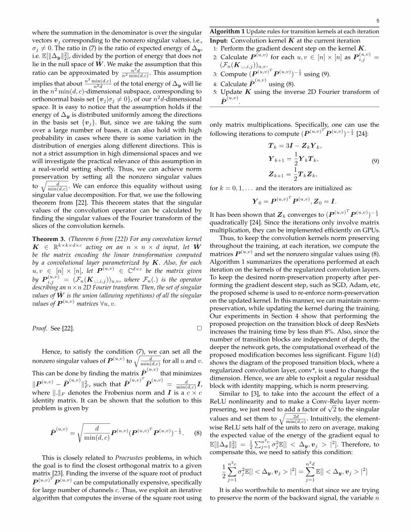
Algorithm 1 Update rules for transition kernels at each iteration

Input: Convolution kernel K at the current iteration1: Perform the gradient descent step on the kernel K.2: Calculate P (u,v) for each u, v ∈ [n] × [n] as P (u,v)

i,j =(Fn(K :,:,i,j))u,v .

3: Compute (P (u,v)TP (u,v))−12 using (9).

4: Calculate P(u,v)

using (8).5: Update K using the inverse 2D Fourier transform of

P(u,v)

.

only matrix multiplications. Specifically, one can use thefollowing iterations to compute (P (u,v)TP (u,v))−

12 [24]:

T k = 3I −ZkY k,

Y k+1 =1

2Y kT k,

Zk+1 =1

2T kZk,

(9)

for k = 0, 1, . . . and the iterators are initialized as:

Y 0 = P (u,v)TP (u,v),Z0 = I.

It has been shown that Zk converges to (P (u,v)TP (u,v))−12

quadratically [24]. Since the iterations only involve matrixmultiplication, they can be implemented efficiently on GPUs.

Thus, to keep the convolution kernels norm preservingthroughout the training, at each iteration, we compute thematrices P (u,v) and set the nonzero singular values using (8).Algorithm 1 summarizes the operations performed at eachiteration on the kernels of the regularized convolution layers.To keep the desired norm-preservation property after per-forming the gradient descent step, such as SGD, Adam, etc,the proposed scheme is used to re-enforce norm-preservationon the updated kernel. In this manner, we can maintain norm-preservation, while updating the kernel during the training.Our experiments in Section 4 show that performing theproposed projection on the transition block of deep ResNetsincreases the training time by less than 8%. Also, since thenumber of transition blocks are independent of depth, thedeeper the network gets, the computational overhead of theproposed modification becomes less significant. Figure 1(d)shows the diagram of the proposed transition block, where aregularized convolution layer, conv*, is used to change thedimension. Hence, we are able to exploit a regular residualblock with identity mapping, which is norm preserving.

Similar to [3], to take into the account the effect of aReLU nonlinearity and to make a Conv-Relu layer norm-presering, we just need to add a factor of

√2 to the singular

values and set them to√

2dmin(d,c) . Intuitively, the element-

wise ReLU sets half of the units to zero on average, makingthe expected value of the energy of the gradient equal toE[‖∆x‖22] = 1

2

∑n2cj=1 σ

2jE[| < ∆y,vj > |2]. Therefore, to

compensate this, we need to satisfy this condition:

1

2

n2c∑j=1

σ2jE[| < ∆y,vj > |2] =

n2d∑j=1

E[| < ∆y,vj > |2]

It is also worthwhile to mention that since we are tryingto preserve the norm of the backward signal, the variable n

6

in Theorem 3 represents the size of feature map size at theoutput of the convolution.

To evaluate the effectiveness of the proposed projection,we design the following experiment. We perform the pro-jection on the convolution layers of a small 3-layer network.The network consists of 3 convolutional layers, followed byReLU non-linearity. To examine the gradient norm ratio fordifferent number of input and output channels, the secondlayer is a 3×3 convolution with c input channels and d outputchannels. The first and third layers are 1 × 1 convolutionsto change the number of channels and to match the size ofthe input and output layers. Figure 2 shows the gradientnorm ratio, i.e., ‖ ∂E

∂xl+1‖2 to ‖ ∂E∂xl

‖2, for different values of cand d at 10th training epoch on CIFAR-10, with and withoutthe proposed projection. The values are averaged over 10different runs.

It is evident that the proposed projection enhances thenorm preservation of the Conv-ReLU layer, as it moves thegradient norm ratios toward 1. The only failure case is fornetworks with very small c and c� d. This is because, due tothe smaller size of the space, our assumption that the energyof the signal in the n2c dimensional subspace, correspondingto the n2c non-zero singular values, is approximately n2c

n2dof the total energy of the signal, is violated with higherprobability. However, in more practical settings, wherethe number of channels is large and the assumption isheld, the proposed projection performs as expected. Thisexperiment illustrates the validity of our analysis as well asthe effectiveness of the proposed projection for such practicalscenarios. In the next section, we demonstrate the advantagesof the proposed method for image classification task.

4 EXPERIMENTS

To validate our theoretical investigation, presented in Section2, and to empirically demonstrate the behavior and effective-ness of the proposed modifications, we experimented withResidual Network (ResNet) and the proposed ProcrustesResidual Network (ProcResNet) architectures on CIFAR10and CIFAR100 datasets. Training and testing datasets contain50,000 and 10,000 images of visual classes, respectively [25].Standard data augmentation (flipping and shifting), sameas [5], [6], [8], is adopted. Furthermore, channel means andstandard deviations are used to normalize the images. Thenetwork is trained using stochastic gradient descent. Theweights are initialized using the method proposed in [3] andthe initial learning rate is 0.1. Batch size of 128 is used for allthe networks. The weight decay is 10−4 and momentum is0.9. The results are based on the top-1 classification accuracy.

Experiments are performed on three different networkarchitectures: 1) ResNet contains one convolution layer, Lresidual blocks, three of which are transition blocks, andone fully connected layer. Each residual block consists ofthree convolution layers, as depicted in Figure 1(b) andFigure 1(c), resulting in a network of depth 3L + 2. Thisis the same architecture as in [6]. 2) ProcResNet has thesame architecture as ResNet, except the transition layers aremodified, as explained in Section 3. In this design, 3 extraconvolution layers are added to the network. However, wecan use the first convolution layer of the original ResNetdesign to match the dimensions and only add two extra

4

640

128

1

4

2

64

3

4

128

5

256256

0 1 2 3 4 5

(a) With the Proposed Regularization

4

640

128

1

4

2

64

3

4

128

5

256256

(b) Without Regularization

Figure 2: The ratio of gradient norm at output to gradient normat input, i.e., ‖ ∂E

∂xl+1‖2 to ‖ ∂E

∂xl‖2, of a convolution layer for

different number of input and output channels at 10th trainingepoch (a) with, and (b) without the proposed regularization onthe singular values of the convolution.

layers. This leads to a network of depth 3L + 4. 3) Plainnetwork is also same as ResNet without the skip connectionin all the L residual blocks, as shown in Figure 1(e).

Furthermore, to decrease the computational burden ofthe proposed regularization, we perform the projection, asdescribed in Section 3, every 2 iterations. This reducesthe computation time significantly without hurting theperformance much. In this setting, performing the proposedregularization increases the training time for ResNet164about 7.6%. However, since we perform the regularizationonly on three blocks, regardless of the depth, as the networkbecomes deeper the computational overhead becomes lesssignificant. For example, implementing the same projectionson ResNet1001 increases the training time by only 3.5%. Thisis significantly less computation compared to regularizationusing SVD, which leads to 53% and 23% training timeoverhead for ResNet164 and ResNet1001, respectively1.

4.1 Norm-Preservation

In the first set of experiments, the behavior of differentarchitectures is studied as the function of network depth.To this end, the ratio of gradient norm at output to gradientnorm at input, i.e., ‖ ∂E

∂xl+1‖2 to ‖ ∂E∂xl

‖2, is captured for all the

1. An implementation of ProcResNet is provided here: https://github.com/zaeemzadeh/ProcResNet

7

100

101

102

10-2

10-1

100

101

102

(a) Plain20

100

101

102

10-2

10-1

100

101

102

(b) ResNet20

100

101

102

10-2

10-1

100

101

102

(c) ProcResNet22

100

101

102

10-2

10-1

100

101

102

(d) Plain83

100

101

102

10-2

10-1

100

101

102

(e) ResNet83

100

101

102

10-2

10-1

100

101

102

(f) ProcResNet85

100

101

102

10-2

10-1

100

101

102

(g) Plain164

100

101

102

10-2

10-1

100

101

102

(h) ResNet164

100

101

102

10-2

10-1

100

101

102

(i) ProcResNet166

Figure 3: Training on CIFAR10. Gradient norm ratio over the first 100 epochs for transition blocks (blocks that change thedimension) and non-transition blocks (blocks that do not change the dimension). The darker color lines represent the transitionblocks and the lighter color lines represent the non-transition blocks. The proposed regularization enhances the norm-preservationof the transition blocks effectively.

residual blocks2, both transition and non-transition. Figure3 shows the ratios for different blocks over training epochs.We ran the training for 100 epochs, without decaying thelearning rate. Plain network (Figure 3.(g)) with 164 layersbecame numerically unstable and the training procedurestopped after 10 epochs.

Several interesting observations can be made from thisexperiment:• This experiment emphasizes the fact that one needs more

than careful initialization to make the network norm-preserving. Although the plain network is initially norm-preserving, the range of the gradient norm ratios becomesvery large and diverges from 1, as the parameters areupdated. However, ResNet and ProcResNet are able toenforce the norm-preservation during training procedureby using identity skip connection.

2. In Plain architecture, which does not have skip connections, thegradient norm ratio is obtained at the input and output of its buildingblocks as depicted in Figure 1(e).

• As the networks become deeper, the plain network be-comes less norm preserving, which leads to numericalinstability, optimization difficulty, and performance degra-dation. On the contrary, the non-transition blocks, theblocks with identity mapping as skip connection, of ResNetand ProcResNet become extra norm preserving. This is inline with our theoretical investigation for linear residualnetworks, which states that as we stack more residualblocks the network becomes extra norm-preserving.

• Comparing Plain83 (Figure 3(d)) and Plain164 (Figure 3(h))networks, it can be observed that most of the blocks behavefairly similar, except one transition block. Specifically, inPlain83, the gradient norm ratio of the first transition blockgoes up to 100 in the first few epochs. But it eventuallydecreases and the network is able to converge. On theother hand, in Plain164, the gradient norm ratio of thesame block becomes too large, which makes the networkunable to converge. Hence, a single block is enough tomake the optimization difficult and numerically unstable.

8

This highlights the fact that it is necessary to enforce norm-preservation on all the blocks.

• In ResNet83 (Figure 3(e)) and ResNet164 (Figure 3(h)), itis easy to notice that only 3 transition blocks are not normpreserving. As mentioned earlier, due to multiplicativeeffect, the magnitude of the gradient will not be preservedbecause of these few blocks.

• The behaviors of ResNet and Plain architectures are fairlysimilar for depth of 20. This was somehow expected, sinceit is known that the performance gain achieved by ResNetis more significant in deeper architectures [5]. However,even for depth of 20, ProcResNet architecture is more normpreserving.

• In ProcResNet, the only block that is less norm preservingis the first transition block, where the 3 RGB channelsare transformed into 64 channels. This is because, as wehave shown in Figure 2, under such condition, where thenumber of input channels is very small, the assumptionthat energy of the gradient signal in the low-dimensionalsubspace, corresponding to the few non-zero singularvalues, is approximately proportional to the size of thesubspace is violated with higher probability.

• The ratios of the gradients for all networks, even thePlain network, are roughly concentrated around 1, whiletraining is stable. This shows that some degree of normpreservation exists in any stable network. However, asclear in the Plain network, such biases of the optimizer isnot enough and we need skip connections to enforce normpreservation throughout training and to enjoy its desirableproperties. Furthermore, although the transition blocks ofResNet tend to converge to be more norm preserving, ourproposed modification enforces this property for all theepochs, which leads to stability and performance gain, aswill be discussed shortly.

This experiment both validates our theoretical argumentsand clarifies some of the inner workings of ResNet archi-tecture, and also shows the effectiveness of the proposedmodifications in ProcResNet. It is evident that, as stated inTheorem 1, addition of identity skip connection makes theblocks increasingly extra norm-preserving, as the networkbecomes deeper. Furthermore, we have been able to enhancenorm-preserving property by applying the changes proposedin Section 3.

4.2 Optimization Stability and Learning Dynamics

In the next set of experiments, numerical stability andlearning dynamics of different architectures is examined. Forthat, loss and classification error, in both training and testingphases, are depicted in Figure 4. This experiment illustratesthat how optimization stability of deep networks is improvedsignificantly, and how it can be further improved by havingnorm preservation in mind during the design procedure.

As depicted in Figure 4, unlike the plain network,training error and loss curves corresponding to ResNet andProcResNet architectures are consistently decreasing as thenumber of layers increases, which was the main motivationbehind proposing residual blocks [5]. Moreover, Figure 4(a)and Figure 4(d) show that the plain networks have a poorgeneralization performance. The fluctuations in testing errorshows that the points along the optimization path of the

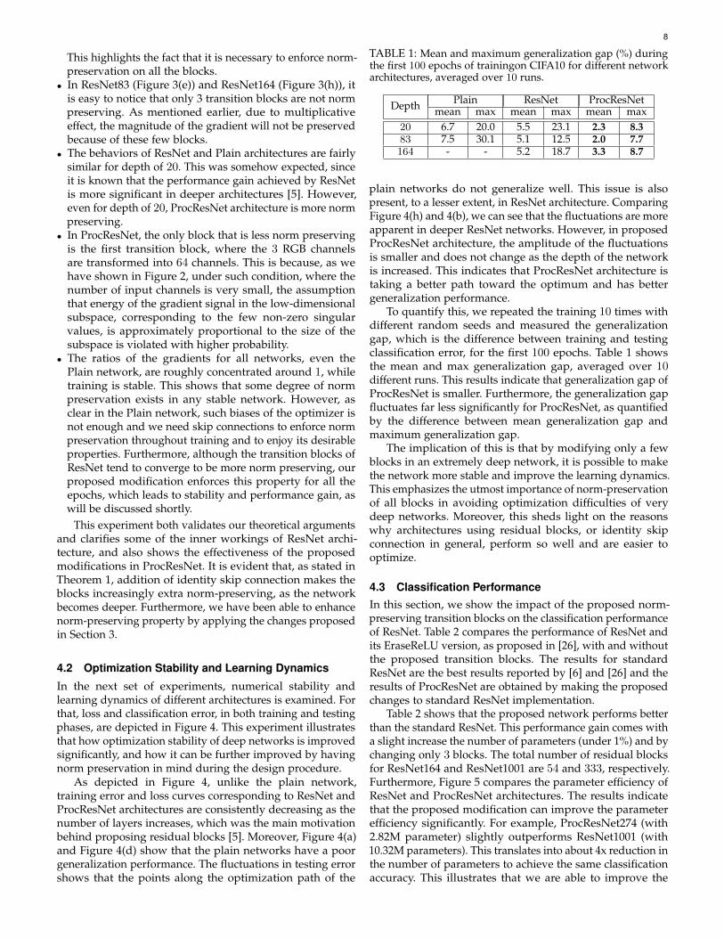
TABLE 1: Mean and maximum generalization gap (%) duringthe first 100 epochs of trainingon CIFA10 for different networkarchitectures, averaged over 10 runs.

Depth Plain ResNet ProcResNetmean max mean max mean max

20 6.7 20.0 5.5 23.1 2.3 8.383 7.5 30.1 5.1 12.5 2.0 7.7164 - - 5.2 18.7 3.3 8.7

plain networks do not generalize well. This issue is alsopresent, to a lesser extent, in ResNet architecture. ComparingFigure 4(h) and 4(b), we can see that the fluctuations are moreapparent in deeper ResNet networks. However, in proposedProcResNet architecture, the amplitude of the fluctuationsis smaller and does not change as the depth of the networkis increased. This indicates that ProcResNet architecture istaking a better path toward the optimum and has bettergeneralization performance.

To quantify this, we repeated the training 10 times withdifferent random seeds and measured the generalizationgap, which is the difference between training and testingclassification error, for the first 100 epochs. Table 1 showsthe mean and max generalization gap, averaged over 10different runs. This results indicate that generalization gap ofProcResNet is smaller. Furthermore, the generalization gapfluctuates far less significantly for ProcResNet, as quantifiedby the difference between mean generalization gap andmaximum generalization gap.

The implication of this is that by modifying only a fewblocks in an extremely deep network, it is possible to makethe network more stable and improve the learning dynamics.This emphasizes the utmost importance of norm-preservationof all blocks in avoiding optimization difficulties of verydeep networks. Moreover, this sheds light on the reasonswhy architectures using residual blocks, or identity skipconnection in general, perform so well and are easier tooptimize.

4.3 Classification PerformanceIn this section, we show the impact of the proposed norm-preserving transition blocks on the classification performanceof ResNet. Table 2 compares the performance of ResNet andits EraseReLU version, as proposed in [26], with and withoutthe proposed transition blocks. The results for standardResNet are the best results reported by [6] and [26] and theresults of ProcResNet are obtained by making the proposedchanges to standard ResNet implementation.

Table 2 shows that the proposed network performs betterthan the standard ResNet. This performance gain comes witha slight increase the number of parameters (under 1%) and bychanging only 3 blocks. The total number of residual blocksfor ResNet164 and ResNet1001 are 54 and 333, respectively.Furthermore, Figure 5 compares the parameter efficiency ofResNet and ProcResNet architectures. The results indicatethat the proposed modification can improve the parameterefficiency significantly. For example, ProcResNet274 (with2.82M parameter) slightly outperforms ResNet1001 (with10.32M parameters). This translates into about 4x reduction inthe number of parameters to achieve the same classificationaccuracy. This illustrates that we are able to improve the

9

0 20 40 60 80 1000

0.5

1

1.5

2

0

10

20

30

40

(a) Plain20

0 20 40 60 80 1000

0.5

1

1.5

2

0

10

20

30

40

(b) ResNet20

0 20 40 60 80 1000

0.5

1

1.5

2

0

10

20

30

40

(c) ProcResNet22

0 20 40 60 80 1000

0.5

1

1.5

2

0

10

20

30

40

(d) Plain83

0 20 40 60 80 1000

0.5

1

1.5

2

0

10

20

30

40

(e) ResNet83

0 20 40 60 80 1000

0.5

1

1.5

2

0

10

20

30

40

(f) ProcResNet85

0 20 40 60 80 1000

0.5

1

1.5

2

2.5

3

0

20

40

60

80

100

(g) Plain164

0 20 40 60 80 1000

0.5

1

1.5

2

0

10

20

30

40

(h) ResNet164

0 20 40 60 80 1000

0.5

1

1.5

2

0

10

20

30

40

(i) ProcResNet166

Figure 4: Loss (black lines) and error (blue lines) during training procedure on CIFAR10. Solid lines represent the test valuesand dotted lines represent the training values. This experiments shows how the residual connections enhance the stability of theoptimization and how the proposed regularization enhances the stability even further.

performance by changing a tiny portion of the networkand emphasizes the importance of norm-preservation inthe performance of neural networks.

Finally, Table 3 investigates the impact of changing thearchitecture, i.e., moving the convolution layer from the skipconnection to before the skip connection, and performingthe proposed regularization, separately. Each of these designcomponents have positive impact on the performance of thenetwork, as both of them enhance the norm preservation ofthe transition block, which further highlights the impact ofnorm preservation on the performance of the network.

5 CONCLUSIONS

This paper theoretically analyzes building blocks of resid-ual networks and demonstrates that adding identity skipconnection makes the residual blocks norm-preserving. Fur-thermore, the norm-preservation is enforced during the

0 2 4 6 8 103

3.5

4

4.5

5

5.5

6

Figure 5: Comparison of the parameter efficiency on CIFAR10between ResNet and ProcResNet.

training procedure, which makes the optimization stableand improves the performance. This is in contrast to ini-

10

TABLE 2: Performance of different methods on CIFAR-10 and CIFAR-100 using moderate data augmentation (flip/translation).The modified transition blocks in ProcResNet can improve the accuracy of ResNet significantly.

Architecture Setting # Params Depth Error (%)CIFAR10 CIFAR100

ResNet [6]pre-activation 1.71M 164 5.46 24.33

10.32M 1001 4.62 22.71

ErasedReLU [26] 1.70M 164 4.65 22.4110.32M 1001 4.10 20.63

ProcResNetpre-activation 1.72M 166 4.75 22.61

10.33M 1003 3.72 19.99

ErasedReLU [26] 1.72M 166 4.53 21.9110.33M 1003 3.42 18.12

TABLE 3: Ablation study on ResNet with 164 layers onCIFAR100.

Transition Block Projection Error (%)Original No 24.33Modified No 23.06Modified Yes 22.61

tialization techniques, such as [14], which ensure norm-preservation only at the beginning of the training. Our ex-periments validate our theoretical investigation by showingthat (i) identity skip connection results in norm preservation,(ii) residual blocks become extra norm-preserving as thenetwork becomes deeper, and (iii) the training can becomemore stable through enhancing the norm preservation of thenetwork. Our proposed modification of ResNet, ProcrustesResNet, enforces norm-preservation on the transition blocksof the network and is able to achieve better optimizationstability and performance. For that we propose an efficientregularization technique to set the nonzero singular values ofthe convolution operator, without performing singular valuedecomposition. Our findings can be seen as design guidelinesfor very deep architectures. By having norm-preservation inmind, we will be able to train extremely deep networks andalleviate the optimization difficulties of such networks.

6 ACKNOWLEDGEMENTS

This research is based upon work supported in parts bythe National Science Foundation under Grants No. 1741431and CCF-1718195 and the Office of the Director of NationalIntelligence (ODNI), Intelligence Advanced Research ProjectsActivity (IARPA), via IARPA R&D Contract No. D17PC00345.The views, findings, opinions, and conclusions or recom-mendations contained herein are those of the authors andshould not be interpreted as necessarily representing theofficial policies or endorsements, either expressed or implied,of the NSF, ODNI, IARPA, or the U.S. Government. TheU.S. Government is authorized to reproduce and distributereprints for Governmental purposes notwithstanding anycopyright annotation thereon.

REFERENCES

[1] D. Silver, J. Schrittwieser, K. Simonyan, I. Antonoglou, A. Huang,A. Guez, T. Hubert, L. Baker, M. Lai, A. Bolton, Y. Chen, T. Lillicrap,F. Hui, L. Sifre, G. van den Driessche, T. Graepel, and D. Hassabis,“Mastering the game of Go without human knowledge,” Nature,vol. 550, pp. 354–359, 10 2017.

[2] G. F. Montufar, R. Pascanu, K. Cho, and Y. Bengio, “On the Numberof Linear Regions of Deep Neural Networks,” in Advances in NeuralInformation Processing Systems 27 (Z. Ghahramani, M. Welling,C. Cortes, N. D. Lawrence, and K. Q. Weinberger, eds.), pp. 2924–2932, Curran Associates, Inc., 2014.

[3] K. He, X. Zhang, S. Ren, and J. Sun, “Delving Deep into Rectifiers:Surpassing Human-Level Performance on ImageNet Classification,”in 2015 IEEE International Conference on Computer Vision (ICCV),pp. 1026–1034, IEEE, 12 2015.

[4] S. Ioffe and C. Szegedy, “Batch Normalization: Accelerating DeepNetwork Training by Reducing Internal Covariate Shift,” 6 2015.

[5] K. He, X. Zhang, S. Ren, and J. Sun, “Deep Residual Learning forImage Recognition,” in 2016 IEEE Conference on Computer Vision andPattern Recognition (CVPR), pp. 770–778, IEEE, 6 2016.

[6] K. He, X. Zhang, S. Ren, and J. Sun, “Identity mappings in deepresidual networks,” in Lecture Notes in Computer Science (includingsubseries Lecture Notes in Artificial Intelligence and Lecture Notes inBioinformatics), vol. 9908 LNCS, pp. 630–645, Springer, Cham, 102016.

[7] R. K. Srivastava, K. Greff, and J. Schmidhuber, “Training Very DeepNetworks,” 2015.

[8] G. Huang, Z. Liu, L. v. d. Maaten, and K. Q. Weinberger, “DenselyConnected Convolutional Networks,” in 2017 IEEE Conference onComputer Vision and Pattern Recognition (CVPR), pp. 2261–2269,IEEE, 7 2017.

[9] A. E. Orhan and X. Pitkow, “Skip connections eliminate singulari-ties,” in 6th International Conference on Learning Representations, ICLR2018 - Conference Track Proceedings, 1 2018.

[10] M. Hardt and T. Ma, “Identity matters in deep learning,” in 5thInternational Conference on Learning Representations, ICLR 2017 -Conference Track Proceedings, 11 2017.

[11] K. Kawaguchi, “Deep Learning without Poor Local Minima,” 2016.[12] D. Balduzzi, M. Frean, L. Leary, J. P. Lewis, K. W.-D. Ma, and

B. McWilliams, “The Shattered Gradients Problem: If resnets arethe answer, then what is the question?,” 7 2017.

[13] A. Veit, M. J. Wilber, and S. Belongie, “Residual Networks BehaveLike Ensembles of Relatively Shallow Networks,” in Advances inNeural Information Processing Systems 29 (D. D. Lee, M. Sugiyama,U. V. Luxburg, I. Guyon, and R. Garnett, eds.), pp. 550–558, CurranAssociates, Inc., 2016.

[14] X. Glorot and Y. Bengio, “Understanding the difficulty of trainingdeep feedforward neural networks,” 3 2010.

[15] L. Dinh, J. Sohl-Dickstein Google, B. Samy, and B. Google Brain,“Density estimation using Real NVP,” in ICLR, 2017.

[16] A. N. Gomez, M. Ren, R. Urtasun, and R. B. Grosse, “The reversibleresidual network: Backpropagation without storing activations,” inAdvances in Neural Information Processing Systems, 2017.

[17] J. Behrmann, W. Grathwohl, R. T. Chen, D. Duvenaud, and J. H.Jacobsen, “Invertible residual networks,” in 36th InternationalConference on Machine Learning, ICML 2019, 2019.

[18] P. L. Bartlett, S. N. Evans, and P. M. Long, “Representingsmooth functions as compositions of near-identity functionswith implications for deep network optimization,” arXiv preprintarXiv:1804.05012, 4 2018.

[19] K. Kawaguchi and Y. Bengio, “Depth with nonlinearity creates nobad local minima in ResNets,” Neural Networks, 2019.

[20] S. Gunasekar, J. D. Lee, N. Srebro, and D. Soudry, “Implicit bias ofgradient descent on linear convolutional networks,” in Advances inNeural Information Processing Systems, 2018.

11

[21] E. Hoffer, I. Hubara, and D. Soudry, “Train longer, generalize better:Closing the generalization gap in large batch training of neuralnetworks,” in Advances in Neural Information Processing Systems,2017.

[22] H. Sedghi, V. Gupta, and P. M. Long, “The Singular Values ofConvolutional Layers,” in International Conference on LearningRepresentations, 2019.

[23] J. C. Gower, G. B. Dijksterhuis, and others, Procrustes problems,vol. 30. Oxford University Press on Demand, 2004.

[24] N. J. Higham, “Stable iterations for the matrix square root,”Numerical Algorithms, vol. 15, no. 2, pp. 227–242, 1997.

[25] A. Krizhevsky and G. Hinton, “Learning multiple layers of featuresfrom tiny images.(2009),” tech. rep., 2009.

[26] X. Dong, G. Kang, K. Zhan, and Y. Yang, “EraseReLU: A SimpleWay to Ease the Training of Deep Convolution Neural Networks,”arXiv preprint arXiv:1709.07634, 2017.

[27] N. A. Derzko and A. M. Pfeffer, “Bounds for the Spectral Radius ofa Matrix,” Mathematics of Computation, vol. 19, p. 62, 4 1965.

Alireza Zaeemzadeh (S‘11) received the B.S.degree in electrical engineering from the Uni-versity of Tehran, Tehran, Iran, in 2014. He iscurrently working toward the Ph.D. degree inelectrical engineering at the University of CentralFlorida. His current research interests lie in theareas of machine learning, linear algebra, andoptimization. Alireza‘s awards and honors includeUniversity of Central Florida Multidisciplinary Doc-toral Fellowship and Graduate Dean’s Fellowship.

Nazanin Rahnavard (S‘97-M‘10-SM’19) re-ceived her Ph.D. in the School of Electrical andComputer Engineering at the Georgia Institute ofTechnology, Atlanta, in 2007. She is currently anAssociate Professor in the Department of Electri-cal and Computer Engineering at the University ofCentral Florida, Orlando, Florida. Dr. Rahnavardis the recipient of NSF CAREER award in 2011and 2020 UCF’s College of Engineering and Com-puter Science Excellence in Research Award.She has interest and expertise in a variety of

research topics in the communications, networking, signal processing,and machine learning areas. She serves on the editorial board of theElsevier Journal on Computer Networks (COMNET) and on the TechnicalProgram Committee of several prestigious international conferences.

Mubarak Shah , the UCF Trustee chair professor,is the founding director of the Center for Researchin Computer Vision at the University of CentralFlorida (UCF). He is a fellow of the NAI, IEEE,AAAS, IAPR, and SPIE. He is an editor of aninternational book series on video computing,was editor-in-chief of Machine Vision and Appli-cations journal, and an associate editor of ACMComputing Surveys journal. He was the programcochair of CVPR 2008, an associate editor of theIEEE T-PAMI, and a guest editor of the special

issue of the International Journal of Computer Vision on Video Computing.His research interests include video surveillance, visual tracking, humanactivity recognition, visual analysis of crowded scenes, video registration,UAV video analysis, and so on. He has served as an ACM distinguishedspeaker and IEEE distinguished visitor speaker. He is a recipient of ACMSIGMM Technical Achievement award; IEEE Outstanding EngineeringEducator Award; Harris Corporation Engineering Achievement Award; anhonorable mention for the ICCV 2005 Where Am I? Challenge Problem;2013 NGA Best Research Poster Presentation; 2nd place in GrandChallenge at the ACM Multimedia 2013 conference; and runner up for thebest paper award in ACM Multimedia Conference in 2005 and 2010. AtUCF he has received Pegasus Professor Award; University DistinguishedResearch Award; Faculty Excellence in Mentoring Doctoral Students;Scholarship of Teaching and Learning award; Teaching Incentive Programaward; Research Incentive Award.

12

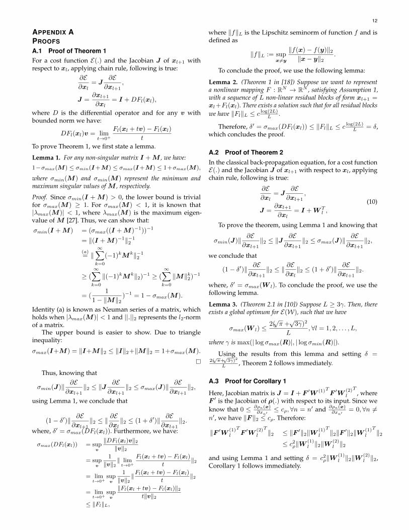
APPENDIX APROOFS

A.1 Proof of Theorem 1For a cost function E(.) and the Jacobian J of xl+1 withrespect to xl, applying chain rule, following is true:

∂E∂xl

= J∂E

∂xl+1,

J =∂xl+1

∂xl= I +DFl(xl),

where D is the differential operator and for any v withbounded norm we have:

DFl(xl)v = limt→0+

Fl(xl + tv)− Fl(xl)t

To prove Theorem 1, we first state a lemma.

Lemma 1. For any non-singular matrix I +M , we have:1−σmax(M) ≤ σmin(I+M) ≤ σmax(I+M) ≤ 1+σmax(M),

where σmin(M) and σmin(M) represent the minimum andmaximum singular values of M , respectively.

Proof. Since σmin(I + M) > 0, the lower bound is trivialfor σmax(M) ≥ 1. For σmax(M) < 1, it is known that|λmax(M)| < 1, where λmax(M) is the maximum eigen-value of M [27]. Thus, we can show that:

σmin(I +M) = (σmax((I +M)−1))−1

= ‖(I +M)−1‖−12

(a)= ‖

∞∑k=0

(−1)kMk‖−12

≥ (∞∑k=0

‖(−1)kMk‖2)−1 ≥ (∞∑k=0

‖M‖k2)−1

= (1

1− ‖M‖2)−1 = 1− σmax(M).

Identity (a) is known as Neuman series of a matrix, whichholds when |λmax(M)| < 1 and ||.||2 represents the l2-normof a matrix.

The upper bound is easier to show. Due to triangleinequality:

σmax(I+M) = ‖I+M‖2 ≤ ‖I‖2+‖M‖2 = 1+σmax(M).

Thus, knowing that

σmin(J)‖ ∂E∂xl+1

‖2 ≤ ‖J∂E

∂xl+1‖2 ≤ σmax(J)‖ ∂E

∂xl+1‖2,

using Lemma 1, we conclude that

(1− δ′)‖ ∂E∂xl+1

‖2 ≤ ‖∂E∂xl‖2 ≤ (1 + δ′)‖ ∂E

∂xl+1‖2.

where, δ′ = σmax(DFl(xl)). Furthermore, we have:

σmax(DFl(xl)) = supv

‖DFl(xl)v‖2‖v‖2

= supv

1

‖v‖2‖ lim

t→0+

Fl(xl + tv)− Fl(xl)

t‖2

= limt→0+

supv

1

‖v‖2‖Fl(xl + tv)− Fl(xl)

t‖2

= limt→0+

supv

‖Fl(xl + tv)− Fl(xl)‖2t‖v‖2

≤ ‖Fl‖L,

where ‖f‖L is the Lipschitz seminorm of function f and isdefined as

‖f‖L := supx6=y

‖f(x)− f(y)‖2‖x− y‖2

.

To conclude the proof, we use the following lemma:

Lemma 2. (Theorem 1 in [18]) Suppose we want to representa nonlinear mapping F : RN → RN , satisfying Assumption 1,with a sequence of L non-linear residual blocks of form xl+1 =xl+Fl(xl). There exists a solution such that for all residual blockswe have ‖Fl‖L ≤ c log(2L)L .

Therefore, δ′ = σmax(DFl(xl)) ≤ ‖Fl‖L ≤ c log(2L)L = δ,which concludes the proof.

A.2 Proof of Theorem 2In the classical back-propagation equation, for a cost functionE(.) and the Jacobian J of xl+1 with respect to xl, applyingchain rule, following is true:

∂E∂xl

= J∂E

∂xl+1,

J =∂xl+1

∂xl= I +W T

l ,

(10)

To prove the theorem, using Lemma 1 and knowing that

σmin(J)‖ ∂E∂xl+1

‖2 ≤ ‖J∂E

∂xl+1‖2 ≤ σmax(J)‖ ∂E

∂xl+1‖2,

we conclude that

(1− δ′)‖ ∂E∂xl+1

‖2 ≤ ‖∂E∂xl‖2 ≤ (1 + δ′)‖ ∂E

∂xl+1‖2.

where, δ′ = σmax(W l). To conclude the proof, we use thefollowing lemma.

Lemma 3. (Theorem 2.1 in [10]) Suppose L ≥ 3γ. Then, thereexists a global optimum for E(W), such that we have

σmax(W l) ≤2(√π +√

3γ)2

L,∀l = 1, 2, . . . , L,

where γ is max(| log σmax(R)|, | log σmin(R)|).

Using the results from this lemma and setting δ =2(√π+√3γ)2

L , Theorem 2 follows immediately.

A.3 Proof for Corollary 1

Here, Jacobian matrix is J = I + F ′W (1)TF ′W(2)l

T, where

F ′ is the Jacobian of ρ(.) with respect to its input. Since weknow that 0 ≤ ∂ρn(x)

∂xn′≤ cρ,∀n = n′ and ∂ρn(x)

∂xn′= 0,∀n 6=

n′, we have ‖F ‖2 ≤ cρ. Therefore:

‖F ′W (1)l

TF ′W

(2)l

T‖2 ≤ ‖F ′‖2‖W (1)

l

T‖2‖F ′‖2‖W (1)

l

T‖2

≤ c2ρ‖W(1)l ‖2‖W

(2)l ‖2

and using Lemma 1 and setting δ = c2ρ‖W(1)l ‖2‖W

(2)l ‖2,

Corollary 1 follows immediately.