1

On the Positive Effect of Delay on the Rate of Convergence ofa Class of Linear Time-Delayed Systems

Hossein Moradian and Solmaz S. Kia

Abstract—This paper is a comprehensive study of a long observedphenomenon of increase in the stability margin and so the rate ofconvergence of a class of linear systems due to time delay. We useLambert W function to determine (a) in what systems the delaycan lead to increase in the rate of convergence, (b) the exact rangeof time delay for which the rate of convergence is greater thanthat of the delay free system, and (c) an estimate on the valueof the delay that leads to the maximum rate of convergence.For the special case when the system matrix eigenvalues areall negative real numbers, we expand our results to show thatthe rate of convergence in the presence of delay depends onlyon the eigenvalues with minimum and maximum real parts.Moreover, we determine the exact value of the maximum rateof convergence and the corresponding maximizing time delay.We demonstrate our results through a numerical example on thepractical application in accelerating an agreement algorithm fornetworked systems by use of a delayed feedback.

Keywords—Linear Time-delayed Systems, Rate of Convergence,Lambert Function, Accelerated Static Average Consensus

I. INTRODUCTION

In this paper, we study the effect of a fixed time delay τ ∈ R>0

on the rate of convergence of the retarded time-delayed systemx(t) = Ax(t− τ), (1a)x(t) = φ(t), t ∈ [−τ, 0], (1b)

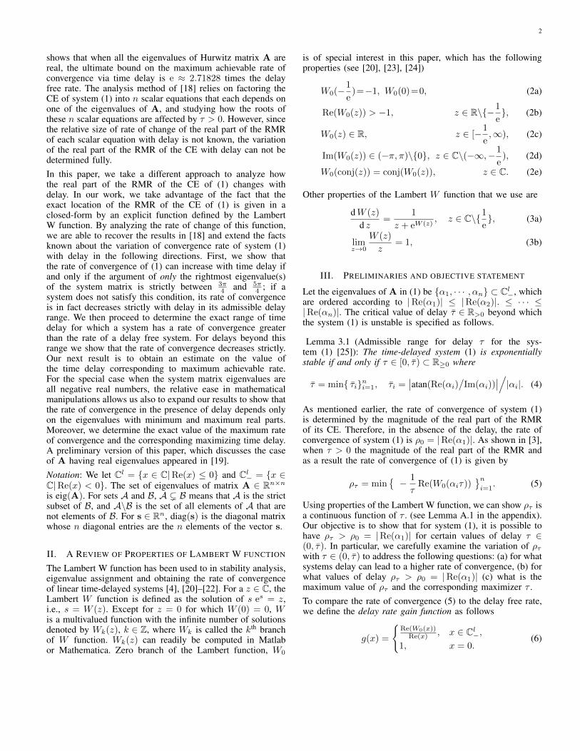
where x(t) ∈ Rn is the state variable at time t, φ(t) is aspecified pre-shape function and A is a Hurwitz matrix.For this system, the continuity stability property theorem forlinear time-delayed systems [1, Proposition 3.1] guaranteesthe existence of the connected admissible range of delay,[0, τ) ⊂ R> 0, for which the exponential stability is preserved.Moreover, the critical value of delay τ > 0, beyond which thesystem is unstable, is the smallest value of the time delay forwhich the rightmost root (RMR) of the characteristic equation(CE) of (1) is on the imaginary axis for the first time. However,as shown in Fig. 1, for some systems the RMR of the CE isnot necessarily traversing monotonically towards the right halfcomplex plane as τ increases. For those systems, contrary tointuition, for certain ranges of delay the rate of convergenceis greater than the delay free case (recall that the exact valueof the worst convergence rate of system (1) is determined bythe magnitude of the real part of the RMR of its CE [2], [3]).For system (1), when τ=0, the RMR of the CE is the rightmosteigenvalue of A, and when τ >0, it can be specified by use of

The authors are with the Department of Mechanical and AerospaceEngineering, University of California Irvine, Irvine, CA 92697,{hmoradia,solmaz}@uci.edu. This work is supported byNSF CAREER grant ECCS 1653838.

0

1

012

case (I)

case (II)

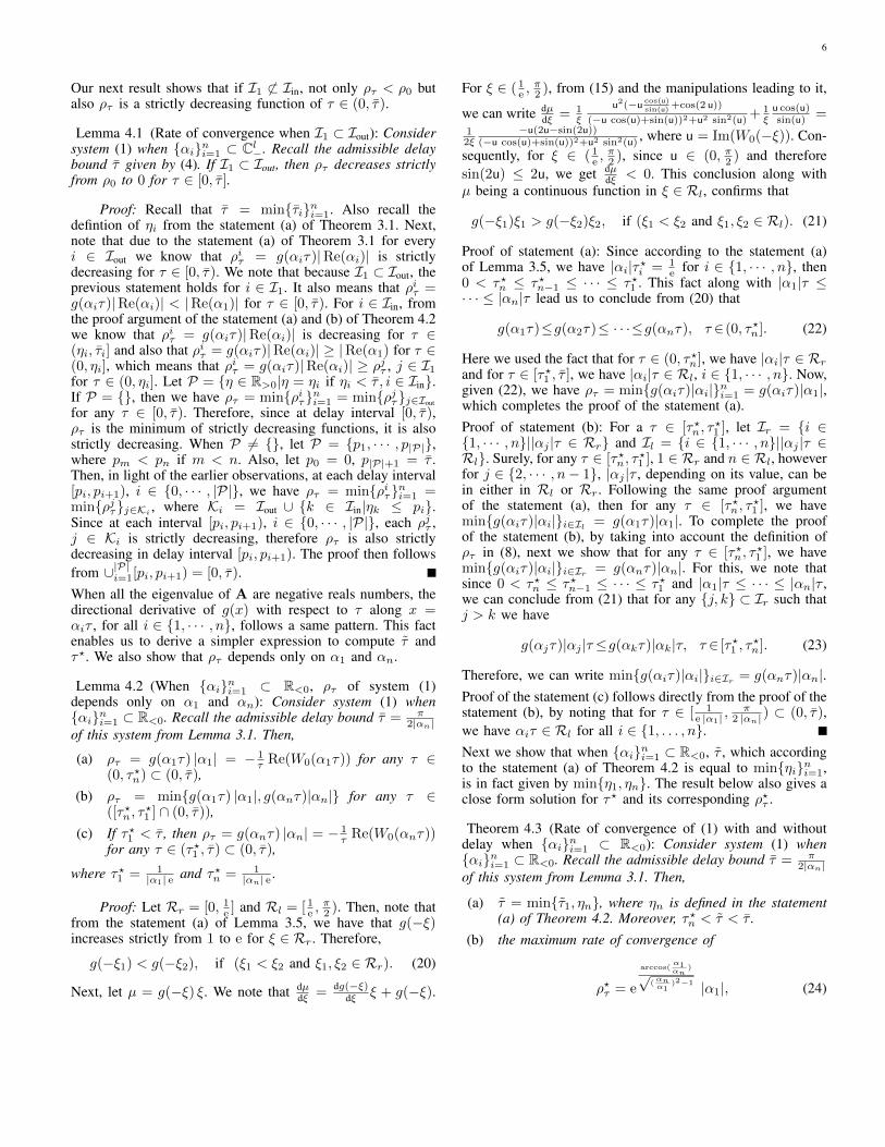
Fig. 1: The normalized real part of the RMR srτ of the CE forthe Laplacian dynamics corresponding to Case (I) and Case (II) inSection V vs. τ ∈ [0, 1]. Since Re(srτ )/Re(sr0)=ρτ/ρ0, we can seethat for the system in Case (I) the rate of convergence can increasewith time delay but this is not the case for the system in Case (II).

the Lambert W function [4]. There are also other methods toestimate the rate of convergence of system (1) [5]–[9]. Despiteabundance of literature on determining the convergence rateof linear systems for a given amount of time delay [1], [5]–[11], there are very few results that address how the rate ofconvergence varies with time delay. In this paper, we aim touse analytical analysis of the variation of rate of convergencevs. time delay to investigate (a) in what type of system (1) thedelay can lead to increase in the rate of convergence, (b) theexact range of time delay for which the rate of convergence isgreater than that of the delay free system, and (c) an estimateon the value of the delay that leads to the maximum rate of con-vergence. This study extends our fundamental understandingof the internal dynamics of linear time-delay systems, and isuseful in identifying rules that facilitate design of systems withfast response and improved stability margin in the presenceof non-zero time delay. A practical application of our resultsis in design of accelerated form of the average consensus(agreement) algorithms [12] in network systems, which wedemonstrate in Section V. Agreement algorithms in networksystems play a crucial role in facilitating many cooperativetasks (see [12], [13] for examples), and their fast convergenceis always desired.Increase of stability margin and the rate of convergence of lin-ear systems with delay has been observed in the literature [14]–[18]. However, the mathematics behind this phenomenon is notfully understood. This is due to the technical challenges thatemanates from the fact that the CE of linear time delayedsystems is transcendental and have an infinite number of rootsin the complex plane. For system (1), [18] offers a set ofinteresting insights into the problem. The main result of [18]states that if all the eigenvalues of A are stable and havein magnitude larger real part than imaginary part (argumentof all the eigenvalues of A are in ( 3π

4 ,5π4 )), the magnitude

of the real part of the RMR of the CE and consequently theconvergence rate of system (1) increases with delay. Also, [18]

arX

iv:1

812.

0403

0v2

[cs

.MA

] 2

0 Ju

l 201

9

2

shows that when all the eigenvalues of Hurwitz matrix A arereal, the ultimate bound on the maximum achievable rate ofconvergence via time delay is e ≈ 2.71828 times the delayfree rate. The analysis method of [18] relies on factoring theCE of system (1) into n scalar equations that each depends onone of the eigenvalues of A, and studying how the roots ofthese n scalar equations are affected by τ > 0. However, sincethe relative size of rate of change of the real part of the RMRof each scalar equation with delay is not known, the variationof the real part of the RMR of the CE with delay can not bedetermined fully.In this paper, we take a different approach to analyze howthe real part of the RMR of the CE of (1) changes withdelay. In our work, we take advantage of the fact that theexact location of the RMR of the CE of (1) is given in aclosed-form by an explicit function defined by the LambertW function. By analyzing the rate of change of this function,we are able to recover the results in [18] and extend the factsknown about the variation of convergence rate of system (1)with delay in the following directions. First, we show thatthe rate of convergence of (1) can increase with time delay ifand only if the argument of only the rightmost eigenvalue(s)of the system matrix is strictly between 3π

4 and 5π4 ; if a

system does not satisfy this condition, its rate of convergenceis in fact decreases strictly with delay in its admissible delayrange. We then proceed to determine the exact range of timedelay for which a system has a rate of convergence greaterthan the rate of a delay free system. For delays beyond thisrange we show that the rate of convergence decreases strictly.Our next result is to obtain an estimate on the value ofthe time delay corresponding to maximum achievable rate.For the special case when the system matrix eigenvalues areall negative real numbers, the relative ease in mathematicalmanipulations allows us also to expand our results to show thatthe rate of convergence in the presence of delay depends onlyon the eigenvalues with minimum and maximum real parts.Moreover, we determine the exact value of the maximum rateof convergence and the corresponding maximizing time delay.A preliminary version of this paper, which discusses the caseof A having real eigenvalues appeared in [19].Notation: We let Cl = {x ∈ C|Re(x) ≤ 0} and Cl− = {x ∈C|Re(x) < 0}. The set of eigenvalues of matrix A ∈ Rn×nis eig(A). For sets A and B, A ( B means that A is the strictsubset of B, and A\B is the set of all elements of A that arenot elements of B. For s ∈ Rn, diag(s) is the diagonal matrixwhose n diagonal entries are the n elements of the vector s.

II. A REVIEW OF PROPERTIES OF LAMBERT W FUNCTION

The Lambert W function has been used to in stability analysis,eigenvalue assignment and obtaining the rate of convergenceof linear time-delayed systems [4], [20]–[22]. For a z ∈ C, theLambert W function is defined as the solution of s es = z,i.e., s = W (z). Except for z = 0 for which W (0) = 0, Wis a multivalued function with the infinite number of solutionsdenoted by Wk(z), k ∈ Z, where Wk is called the kth branchof W function. Wk(z) can readily be computed in Matlabor Mathematica. Zero branch of the Lambert function, W0

is of special interest in this paper, which has the followingproperties (see [20], [23], [24])

W0(−1

e)=−1, W0(0)=0, (2a)

Re(W0(z)) > −1, z ∈ R\{−1

e}, (2b)

W0(z) ∈ R, z ∈ [−1

e,∞), (2c)

Im(W0(z)) ∈ (−π, π)\{0}, z ∈ C\(−∞,−1

e), (2d)

W0(conj(z)) = conj(W0(z)), z ∈ C. (2e)

Other properties of the Lambert W function that we use are

dW (z)

d z=

1

z + eW (z), z ∈ C\{1

e}, (3a)

limz→0

W (z)

z= 1, (3b)

III. PRELIMINARIES AND OBJECTIVE STATEMENT

Let the eigenvalues of A in (1) be {α1, · · · , αn} ⊂ Cl−, whichare ordered according to |Re(α1)| ≤ |Re(α2)|. ≤ · · · ≤|Re(αn)|. The critical value of delay τ ∈ R>0 beyond whichthe system (1) is unstable is specified as follows.

Lemma 3.1 (Admissible range for delay τ for the sys-tem (1) [25]): The time-delayed system (1) is exponentiallystable if and only if τ ∈ [0, τ) ⊂ R≥0 where

τ = min{ τi}ni=1, τi =∣∣atan(Re(αi)

/Im(αi))

∣∣/|αi|. (4)

As mentioned earlier, the rate of convergence of system (1)is determined by the magnitude of the real part of the RMRof its CE. Therefore, in the absence of the delay, the rate ofconvergence of system (1) is ρ0 = |Re(α1)|. As shown in [3],when τ > 0 the magnitude of the real part of the RMR andas a result the rate of convergence of (1) is given by

ρτ = min{− 1

τRe(W0(αiτ))

}ni=1

. (5)

Using properties of the Lambert W function, we can show ρτ isa continuous function of τ . (see Lemma A.1 in the appendix).Our objective is to show that for system (1), it is possible tohave ρτ > ρ0 = |Re(α1)| for certain values of delay τ ∈(0, τ). In particular, we carefully examine the variation of ρτwith τ ∈ (0, τ) to address the following questions: (a) for whatsystems delay can lead to a higher rate of convergence, (b) forwhat values of delay ρτ > ρ0 = |Re(α1)| (c) what is themaximum value of ρτ and the corresponding maximizer τ .To compare the rate of convergence (5) to the delay free rate,we define the delay rate gain function as follows

g(x) =

{Re(W0(x))

Re(x) , x ∈ Cl−,1, x = 0.

(6)

3

-2

-1

0

0123

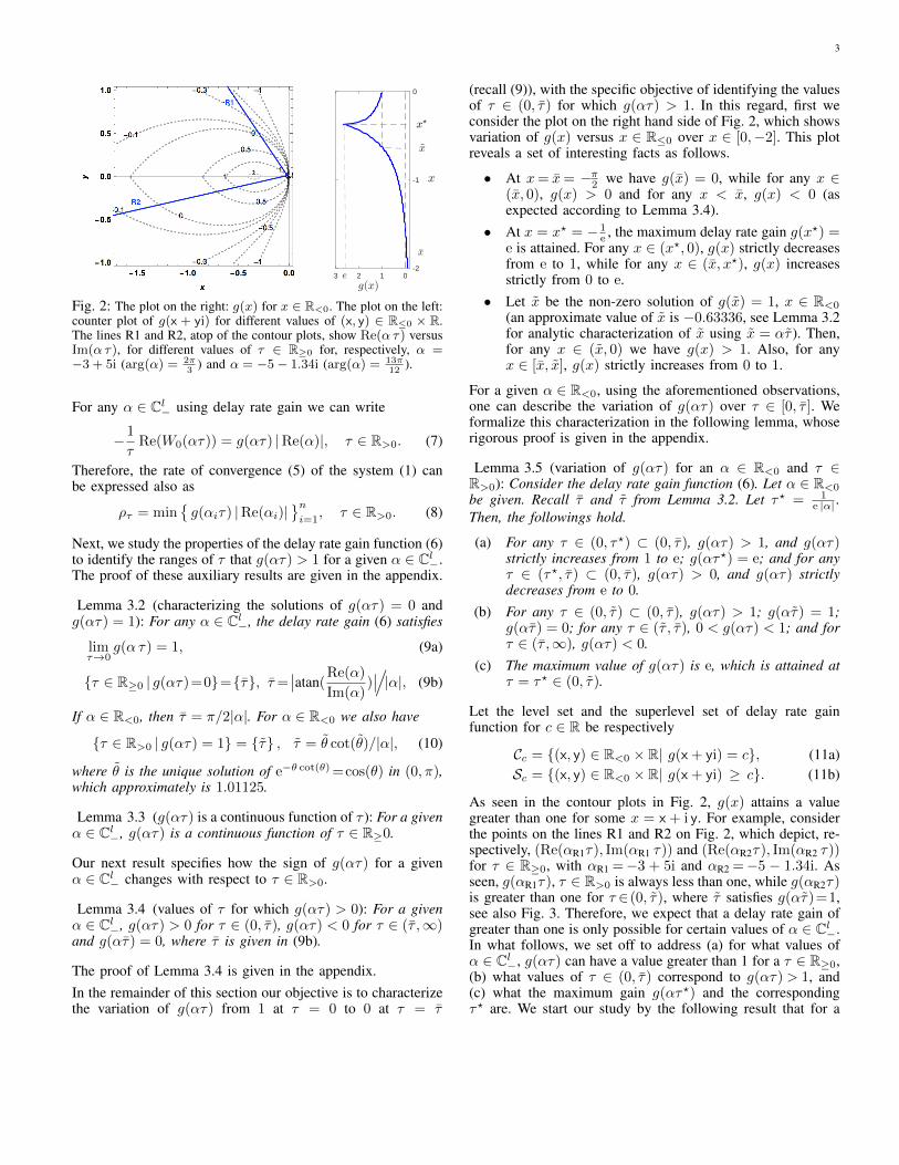
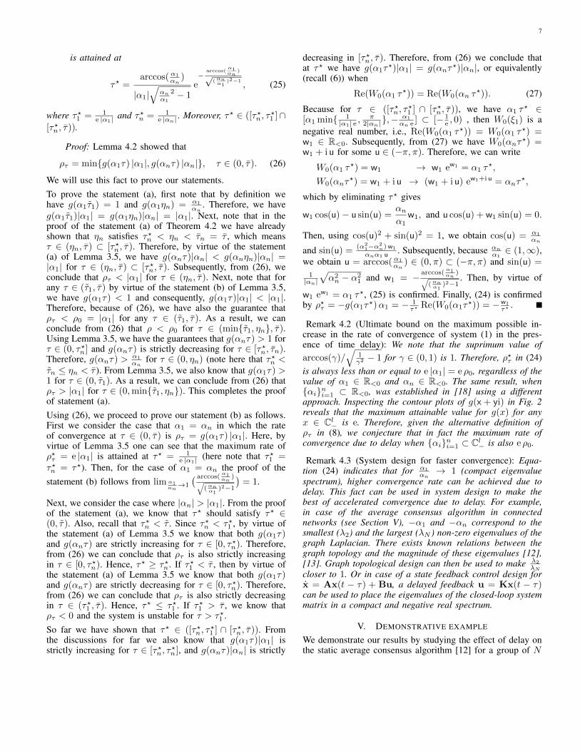
Fig. 2: The plot on the right: g(x) for x ∈ R<0. The plot on the left:counter plot of g(x + yi) for different values of (x, y) ∈ R≤0 × R.The lines R1 and R2, atop of the contour plots, show Re(α τ) versusIm(α τ), for different values of τ ∈ R≥0 for, respectively, α =−3 + 5i (arg(α) = 2π

3) and α = −5− 1.34i (arg(α) = 13π

12).

For any α ∈ Cl− using delay rate gain we can write

−1

τRe(W0(ατ)) = g(ατ) |Re(α)|, τ ∈ R>0. (7)

Therefore, the rate of convergence (5) of the system (1) canbe expressed also as

ρτ = min{g(αiτ) |Re(αi)|

}ni=1

, τ ∈ R>0. (8)

Next, we study the properties of the delay rate gain function (6)to identify the ranges of τ that g(ατ) > 1 for a given α ∈ Cl−.The proof of these auxiliary results are given in the appendix.

Lemma 3.2 (characterizing the solutions of g(ατ) = 0 andg(ατ) = 1): For any α ∈ Cl−, the delay rate gain (6) satisfies

limτ→0

g(α τ) = 1, (9a)

{τ ∈ R≥0 | g(ατ)=0}={τ}, τ=∣∣atan(

Re(α)

Im(α))∣∣/|α|, (9b)

If α ∈ R<0, then τ = π/2|α|. For α ∈ R<0 we also have

{τ ∈ R>0 | g(ατ) = 1} = {τ} , τ = θ cot(θ)/|α|, (10)

where θ is the unique solution of e−θ cot(θ) =cos(θ) in (0, π),which approximately is 1.01125.

Lemma 3.3 (g(ατ) is a continuous function of τ ): For a givenα ∈ Cl−, g(ατ) is a continuous function of τ ∈ R≥0.

Our next result specifies how the sign of g(ατ) for a givenα ∈ Cl− changes with respect to τ ∈ R>0.

Lemma 3.4 (values of τ for which g(ατ) > 0): For a givenα ∈ Cl−, g(ατ) > 0 for τ ∈ (0, τ), g(ατ) < 0 for τ ∈ (τ ,∞)and g(ατ) = 0, where τ is given in (9b).

The proof of Lemma 3.4 is given in the appendix.In the remainder of this section our objective is to characterizethe variation of g(ατ) from 1 at τ = 0 to 0 at τ = τ

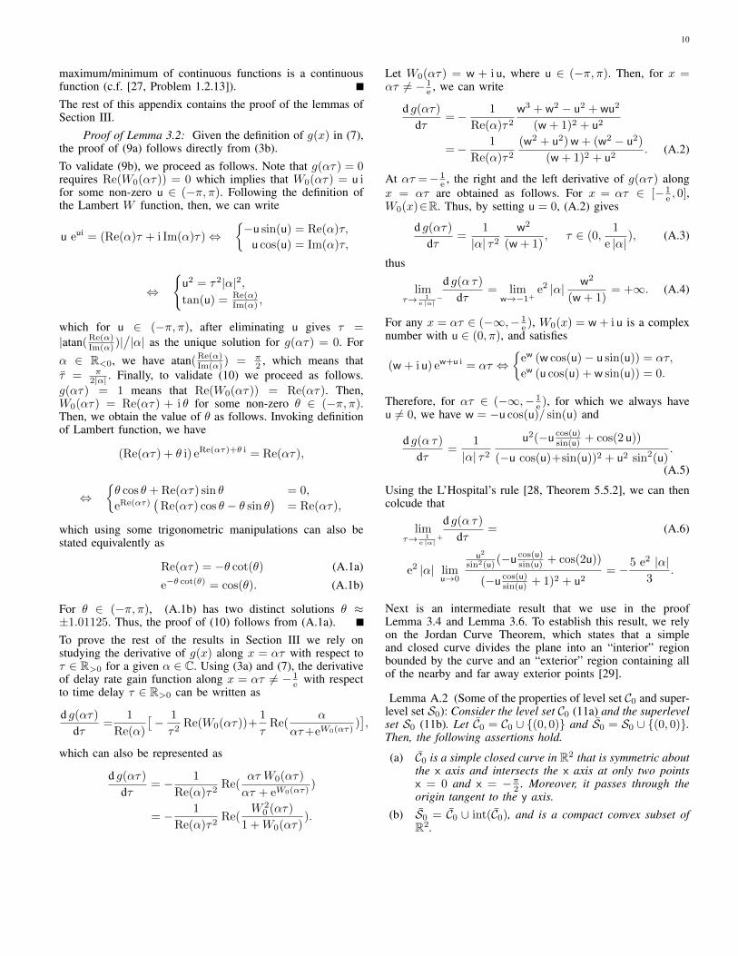
(recall (9)), with the specific objective of identifying the valuesof τ ∈ (0, τ) for which g(ατ) > 1. In this regard, first weconsider the plot on the right hand side of Fig. 2, which showsvariation of g(x) versus x ∈ R≤0 over x ∈ [0,−2]. This plotreveals a set of interesting facts as follows.

• At x= x= −π2 we have g(x) = 0, while for any x ∈(x, 0), g(x) > 0 and for any x < x, g(x) < 0 (asexpected according to Lemma 3.4).

• At x = x? = − 1e , the maximum delay rate gain g(x?) =

e is attained. For any x ∈ (x?, 0), g(x) strictly decreasesfrom e to 1, while for any x ∈ (x, x?), g(x) increasesstrictly from 0 to e.

• Let x be the non-zero solution of g(x) = 1, x ∈ R<0

(an approximate value of x is −0.63336, see Lemma 3.2for analytic characterization of x using x = ατ ). Then,for any x ∈ (x, 0) we have g(x) > 1. Also, for anyx ∈ [x, x], g(x) strictly increases from 0 to 1.

For a given α ∈ R<0, using the aforementioned observations,one can describe the variation of g(ατ) over τ ∈ [0, τ ]. Weformalize this characterization in the following lemma, whoserigorous proof is given in the appendix.

Lemma 3.5 (variation of g(ατ) for an α ∈ R<0 and τ ∈R>0): Consider the delay rate gain function (6). Let α ∈ R<0

be given. Recall τ and τ from Lemma 3.2. Let τ? = 1e |α| .

Then, the followings hold.

(a) For any τ ∈ (0, τ?) ⊂ (0, τ), g(ατ) > 1, and g(ατ)strictly increases from 1 to e; g(ατ?) = e; and for anyτ ∈ (τ?, τ) ⊂ (0, τ), g(ατ) > 0, and g(ατ) strictlydecreases from e to 0.

(b) For any τ ∈ (0, τ) ⊂ (0, τ), g(ατ) > 1; g(ατ) = 1;g(ατ) = 0; for any τ ∈ (τ , τ), 0 < g(ατ) < 1; and forτ ∈ (τ ,∞), g(ατ) < 0.

(c) The maximum value of g(ατ) is e, which is attained atτ = τ? ∈ (0, τ).

Let the level set and the superlevel set of delay rate gainfunction for c ∈ R be respectively

Cc = {(x, y) ∈ R<0 × R| g(x + yi) = c}, (11a)Sc = {(x, y) ∈ R<0 × R| g(x + yi) ≥ c}. (11b)

As seen in the contour plots in Fig. 2, g(x) attains a valuegreater than one for some x = x + i y. For example, considerthe points on the lines R1 and R2 on Fig. 2, which depict, re-spectively, (Re(αR1τ), Im(αR1 τ)) and (Re(αR2τ), Im(αR2 τ))for τ ∈ R≥0, with αR1 =−3 + 5i and αR2 =−5 − 1.34i. Asseen, g(αR1τ), τ ∈ R>0 is always less than one, while g(αR2τ)is greater than one for τ ∈(0, τ), where τ satisfies g(ατ)=1,see also Fig. 3. Therefore, we expect that a delay rate gain ofgreater than one is only possible for certain values of α ∈ Cl−.In what follows, we set off to address (a) for what values ofα ∈ Cl−, g(ατ) can have a value greater than 1 for a τ ∈ R≥0,(b) what values of τ ∈ (0, τ) correspond to g(ατ) > 1, and(c) what the maximum gain g(ατ?) and the correspondingτ? are. We start our study by the following result that for a

4

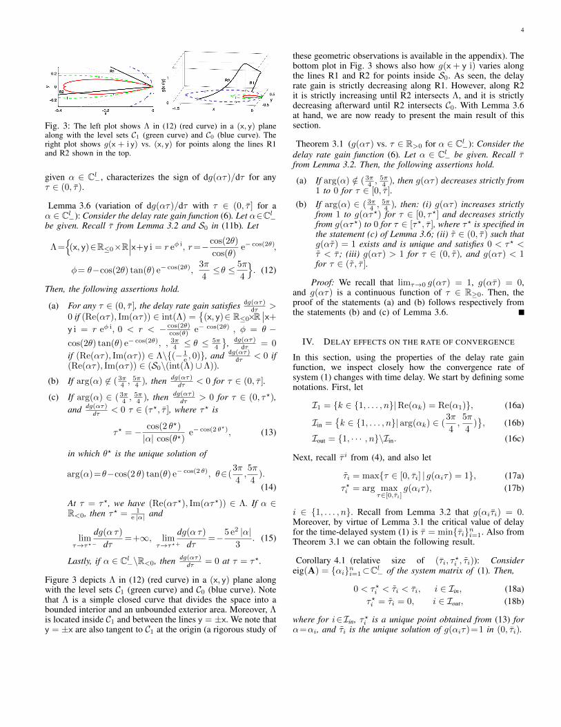
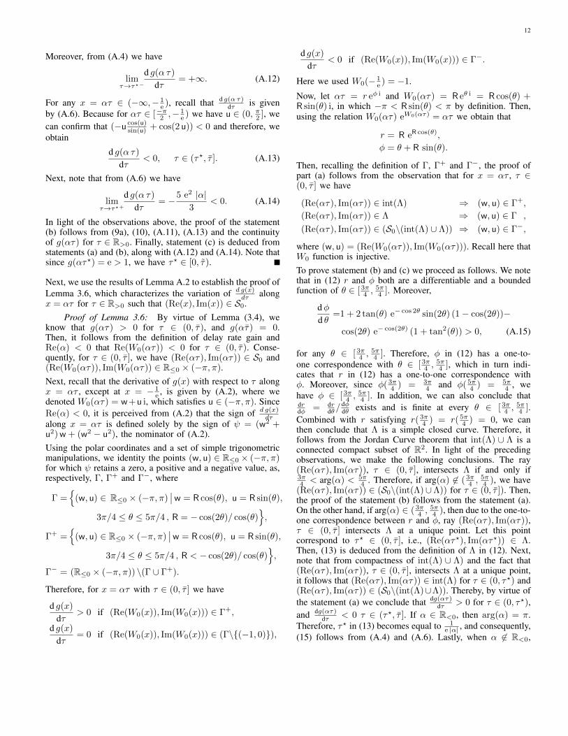
Fig. 3: The left plot shows Λ in (12) (red curve) in a (x, y) planealong with the level sets C1 (green curve) and C0 (blue curve). Theright plot shows g(x + i y) vs. (x, y) for points along the lines R1and R2 shown in the top.

given α ∈ Cl−, characterizes the sign of dg(ατ)/dτ for anyτ ∈ (0, τ).

Lemma 3.6 (variation of dg(ατ)/dτ with τ ∈ (0, τ ] for aα ∈ Cl−): Consider the delay rate gain function (6). Let α∈Cl−be given. Recall τ from Lemma 3.2 and S0 in (11b). Let

Λ={(x, y)∈R≤0×R

∣∣∣x+y i = r eφ i, r=−cos(2θ)

cos(θ)e− cos(2θ),

φ= θ−cos(2θ) tan(θ) e− cos(2θ),3π

4≤θ ≤ 5π

4

}. (12)

Then, the following assertions hold.

(a) For any τ ∈ (0, τ ], the delay rate gain satisfies dg(ατ)dτ >

0 if (Re(ατ), Im(ατ)) ∈ int(Λ) ={

(x, y)∈ R≤0×R∣∣x+

y i = r eφ i, 0 < r < − cos(2θ)cos(θ) e− cos(2θ) , φ = θ −

cos(2θ) tan(θ) e− cos(2θ), , 3π4 ≤ θ ≤

5π4

}, dg(ατ)

dτ = 0

if (Re(ατ), Im(ατ)) ∈ Λ\{(− 1e , 0)}, and dg(ατ)

dτ < 0 if(Re(ατ), Im(ατ)) ∈ (S0\(int(Λ) ∪ Λ)).

(b) If arg(α) 6∈ ( 3π4 ,

5π4 ), then dg(ατ)

dτ < 0 for τ ∈ (0, τ ].

(c) If arg(α) ∈ ( 3π4 ,

5π4 ), then dg(ατ)

dτ > 0 for τ ∈ (0, τ?),and dg(ατ)

dτ < 0 τ ∈ (τ?, τ ], where τ? is

τ? = − cos(2 θ?)

|α| cos(θ?)e− cos(2 θ?), (13)

in which θ? is the unique solution of

arg(α)=θ−cos(2 θ) tan(θ) e− cos(2 θ), θ∈(3π

4,5π

4).

(14)

At τ = τ?, we have (Re(ατ?), Im(ατ?)) ∈ Λ. If α ∈R<0, then τ? = 1

e |α| and

limτ→τ?−

dg(α τ)

dτ=+∞, lim

τ→τ?+dg(α τ)

dτ=−5 e2 |α|

3. (15)

Lastly, if α ∈ Cl−\R<0, then dg(ατ)dτ = 0 at τ = τ?.

Figure 3 depicts Λ in (12) (red curve) in a (x, y) plane alongwith the level sets C1 (green curve) and C0 (blue curve). Notethat Λ is a simple closed curve that divides the space into abounded interior and an unbounded exterior area. Moreover, Λis located inside C1 and between the lines y = ±x. We note thaty = ±x are also tangent to C1 at the origin (a rigorous study of

these geometric observations is available in the appendix). Thebottom plot in Fig. 3 shows also how g(x + y i) varies alongthe lines R1 and R2 for points inside S0. As seen, the delayrate gain is strictly decreasing along R1. However, along R2it is strictly increasing until R2 intersects Λ, and it is strictlydecreasing afterward until R2 intersects C0. With Lemma 3.6at hand, we are now ready to present the main result of thissection.

Theorem 3.1 (g(ατ) vs. τ ∈ R>0 for α ∈ Cl−): Consider thedelay rate gain function (6). Let α ∈ Cl− be given. Recall τfrom Lemma 3.2. Then, the following assertions hold.

(a) If arg(α) /∈ ( 3π4 ,

5π4 ), then g(ατ) decreases strictly from

1 to 0 for τ ∈ [0, τ ].

(b) If arg(α) ∈ ( 3π4 ,

5π4 ), then: (i) g(ατ) increases strictly

from 1 to g(ατ?) for τ ∈ [0, τ?] and decreases strictlyfrom g(ατ?) to 0 for τ ∈ [τ?, τ ], where τ? is specified inthe statement (c) of Lemma 3.6; (ii) τ ∈ (0, τ) such thatg(ατ) = 1 exists and is unique and satisfies 0 < τ? <τ < τ ; (iii) g(ατ) > 1 for τ ∈ (0, τ), and g(ατ) < 1for τ ∈ (τ , τ ].

Proof: We recall that limτ→0 g(ατ) = 1, g(ατ) = 0,and g(ατ) is a continuous function of τ ∈ R≥0. Then, theproof of the statements (a) and (b) follows respectively fromthe statements (b) and (c) of Lemma 3.6.

IV. DELAY EFFECTS ON THE RATE OF CONVERGENCE

In this section, using the properties of the delay rate gainfunction, we inspect closely how the convergence rate ofsystem (1) changes with time delay. We start by defining somenotations. First, let

I1 = {k ∈ {1, . . . , n}|Re(αk) = Re(α1)}, (16a)

Iin ={k ∈ {1, . . . , n}| arg(αk) ∈ (

3π

4,

5π

4)}, (16b)

Iout = {1, · · · , n}\Iin. (16c)

Next, recall τ i from (4), and also let

τi = max{τ ∈ [0, τi] | g(αiτ) = 1}, (17a)τ?i = arg max

τ∈[0,τi]g(αiτ), (17b)

i ∈ {1, . . . , n}. Recall from Lemma 3.2 that g(αiτi) = 0.Moreover, by virtue of Lemma 3.1 the critical value of delayfor the time-delayed system (1) is τ = min{τi}ni=1. Also fromTheorem 3.1 we can obtain the following result.

Corollary 4.1 (relative size of (τi, τ?i , τi)): Consider

eig(A) = {αi}ni=1⊂Cl− of the system matrix of (1). Then,

0 < τ?i < τi < τi, i ∈ Iin, (18a)τ?i = τi = 0, i ∈ Iout, (18b)

where for i∈Iin, τ?i is a unique point obtained from (13) forα=αi, and τi is the unique solution of g(αiτ)=1 in (0, τi).

5

Lastly, we let

τ = max{τ ∈ [0, τ ] | ρτ = |Re(α1)|}, (19a)τ? = arg max

τ∈[0,τ)ρτ , (19b)

ρiτ = g(αiτ)|Re(αi)|, i ∈ {1, · · · , n}. (19c)

With the proper notations at hand, we now present our firstresult, which specifies what system (1) can have a higher rateof convergence in the presence of the time delay.

Theorem 4.1 (Systems for which rate of convergence canincrease by time delay): Consider the linear time-delayedsystem (1) when {αi}ni=1 ⊂ Cl−. Recall the admissible delaybound τ given by (4). Then there always exists a τ ∈ (0, τ)for which ρτ > ρ0 = |Re(α1)| if and only if I1 ⊂ Iin.

Proof: If there exists a j ∈ I1 that is not in Iin, i.e.,arg(αj) /∈ ( 3π

4 ,5π4 ), then by virtue of Lemma (3.4) and the

statement (a) of Theorem 3.1 we know that g(αjτ) < 1 for anyτ ∈ R>0. Subsequently, since |Re(α1)| ≤ · · · ≤ |Re(αn)|,from the definition of the ρτ in (8) we obtain that ρτ <|Re(α1)| for all τ ∈ (0, τ). Now, assume that I1 ⊂ Iin.Then, by virtue of the statement (b) of Theorem 3.1, we knowthat g(αiτ) > 1 for any τ ∈ (0, τi) for i ∈ I1, (recallτi ∈ (0, τi) due to (18)). Subsequently, since g(0) = 1 and|Re(αk)| > |Re(α1)| for k ∈ {1, · · · , n}\I1, then by virtueof Lemma 3.3, there exists a τ ∈ ((0,min{τi}i∈I1) ∩ (0, τ))such that g(αiτ) > 1, i ∈ {1, · · · , n}, for any τ ∈ (0, τ).Then, the proof of the sufficiency of the theorem statementfollows from the definition of ρτ in (8) and its continuity withrespect to τ ∈ R>0.Our next result specifies for what values of time delay asystem, which satisfies the necessary and sufficient conditionof Theorem (4.1), experiences an increase in its rate ofconvergence in the presence of delay. This result also givesthe value of τ and provides an estimate on the value of τ?.

Theorem 4.2 (Ranges of delay for which the rate of conver-gence of (1) increases with delay): Consider the linear time-delayed system (1) when {αi}ni=1 ⊂ Cl−. Recall the admissibledelay bound τ given by (4). Suppose that I1 ⊂ Iin. Then, thefollowing assertions hold.

(a) τ = min{ηi}ni=1, where ηi is the unique solutionof g(αiτ) = |Re(α1)|

|Re(αi)| for τ ∈ (0, τi). Moreover,min{τ?i }ni=1 < τ < τ .

(b) ρτ > ρ0 = |Re(α1)| for τ ∈ (0, τ) ⊂ (0, τ), ρτ = ρ0 =|Re(α1)| at τ = τ and ρτ < ρ0 = |Re(α1)| for τ ∈(τ , τ). Moreover, ρτ decreases strictly with τ ∈ (τ , τ).

(c) τ? ∈([min{τ?i }ni=1,max{τ?i }ni=1] ∩ (0, τ)

)⊂ (0, τ).

Proof: For j ∈ Iout, the statement (a) of Theorem (3.1)guarantees that g(αjτ) is strictly decreasing from 1 to 0 forτ ∈ [0, τj ]. Thus, for j ∈ Iout, given the continuity of g(αjτ)

in τ ∈ [0, τj ] and |Re(α1)||Re(αj)| < 1 (recall that I1 6⊂ Iout),

ηj is a non-zero unique value in (0, τj) at which we haveg(αjηj)|Re(αj)| = |Re(α1)|. Moreover, for j ∈ Iout, we

have g(αjηj)|Re(αj)| < |Re(α1)| for τ ∈ (ηj , τj) andg(αjηj)|Re(αj)| > |Re(α1)| for τ ∈ (0, ηj). Recall alsothat τ?j = 0 for j ∈ Iout. For j ∈ Iin, the statement (b) ofTheorem (3.1) guarantees that g(αjτ) is strictly increasingfrom 1 to its maximum value g(αjτ

?j ) > 1 for τ ∈ (0, τ?j )

and it is strictly decreasing from g(αjτ?j ) > 1 to zero for

τ ∈ [τ?j , τj ]. Thus, for j ∈ Iin, given the continuity of g(αjτ)

in τ ∈ [0, τj ] and |Re(α1)||Re(αj)| ≤ 1 (recall that I1 ⊂ Iin),

ηj is a non-zero unique value in (τ?j , τj) at which we haveg(αjηj)|Re(αj)| = |Re(α1)|. Moreover, for j ∈ Iin, wehave g(αjηj)|Re(αj)| < |Re(α1)| for τ ∈ (ηj , τj) andg(αjηj)|Re(αj)| > |Re(α1)| for τ ∈ (0, ηj). From theaforementioned observations, the validity of the statements (a)and (b) follows from the continuity of ρτ in τ ∈ [0, τ ], itsdefinition (8) and also noting that the minimum of a set ofstrictly decreasing functions is also strictly decreasing.Proof of statement (c): From the statement (b) we can con-clude that 0 < τ? < τ . Given the definition of ρτ in (8),we already know that ρτ? = min{g(αiτ

?) |Re(αi)|}ni=1 ≤g(αiτ

?)|Re(αi)| ≤ g(αiτ?i )|Re(αi)|, i ∈ {1, · · · , n}. There-

fore, τ? ≤ max{τ?i }ni=1. If Iout 6= {}, because of τ?j = 0,j ∈ Iout, then τ? ≥ min{τi}ni=1 is trivial. Now assumeIout = {}. In this case if τ? is not equal to any of the τ?i ,i ∈ {1, · · · , n}, then in order for τ? to be a maximizer point weshould have non-empty I ( {1, · · · , n} and I ( {1, · · · , n}such that dg(αiτ?)

dτ > 0 for i ∈ I and dg(αiτ?)dτ < 0 for i ∈ I.

Consequently, since for τ ∈ (0, τ?i ) we have dg(αiτ)dτ > 0 and

for τ ∈ (τ?i , τi) we have dg(αiτ)dτ < 0, for i ∈ Iin = {1, · · · , n},

then we can conclude that τ? ≥ min{τ?i }ni=1.The statement (c) of Theorem 4.2 provides only an estimate onthe location of τ?. However, by relying on the proof argumentof this statement we can narrow down the search for τ? to aset of discrete points as explained in the remark below.

Remark 4.1 (Candidate points for τ?, when I1 ⊂ Iin): Con-sider system (1) when {αi}ni=1 ⊂ Cl− and I1 ⊂ Iin. From theproof argument of the statement (c) of Theorem 4.2, it followsthat τ? is either a point in T ? = {τ?i }i∈J where J = {i ∈{1, · · · , n}|min{τ?k}nk=1 ≤ τ?i < τ} or an intersection pointof a ρiτ and a ρjτ in τ ∈

([min{τ?k}nk=1,max{τ?k}nk=1]∩(0, τ)

)where dg(αiτ)

dτ > 0 and dg(αjτ)dτ < 0. Based on this obser-

vation, we propose the following procedure to identify thecandidate points for τ?. Let J r = {i ∈ Iin|τ?i ≥ τ}, andJ lj = {i ∈ J |τ?i ≥ τ?j } for any j ∈ J . We note that for

i ∈ J r we have dg(αiτ)dτ > 0 for any τ ∈ (0, τ), and for

any j ∈ J we have dg(αkτ)dτ < 0 for any τ ∈ (τ?j , τ) and

also dg(αkτ)dτ > 0 for any τ ∈ (τ?j , τ

?k ) ⊂ (τ?j , τ), k ∈ J l

j .Now for any j ∈ J let Tj be the set of intersection points ofρjτ with ρkτ , k ∈ (J l

j ∪ J r) for τ ∈ (τ?j , τ) (here note thatthe possible intersection between ρjτ and ρkτ is in fact locatedat (τ?j , τ

?k ) ⊂ (τ?j , τ) for k ∈ I l

j). Then, following the proofargument of the statement (c) of of Theorem 4.2, we haveτ? ∈ (( ∪

j∈JTj) ∪ T ?).

6

Our next result shows that if I1 6⊂ Iin, not only ρτ < ρ0 butalso ρτ is a strictly decreasing function of τ ∈ (0, τ).

Lemma 4.1 (Rate of convergence when I1 ⊂ Iout): Considersystem (1) when {αi}ni=1 ⊂ Cl−. Recall the admissible delaybound τ given by (4). If I1 ⊂ Iout, then ρτ decreases strictlyfrom ρ0 to 0 for τ ∈ [0, τ ].

Proof: Recall that τ = min{τi}ni=1. Also recall thedefintion of ηi from the statement (a) of Theorem 3.1. Next,note that due to the statement (a) of Theorem 3.1 for everyi ∈ Iout we know that ρiτ = g(αiτ)|Re(αi)| is strictlydecreasing for τ ∈ [0, τ). We note that because I1 ⊂ Iout, theprevious statement holds for i ∈ I1. It also means that ρiτ =g(αiτ)|Re(αi)| < |Re(α1)| for τ ∈ [0, τ). For i ∈ Iin, fromthe proof argument of the statement (a) and (b) of Theorem 4.2we know that ρiτ = g(αiτ)|Re(αi)| is decreasing for τ ∈(ηi, τi] and also that ρiτ = g(αiτ)|Re(αi)| ≥ |Re(α1) for τ ∈(0, ηi], which means that ρiτ = g(αiτ)|Re(αi)| ≥ ρjτ , j ∈ I1

for τ ∈ (0, ηi]. Let P = {η ∈ R>0|η = ηi if ηi < τ, i ∈ Iin}.If P = {}, then we have ρτ = min{ρiτ}ni=1 = min{ρjτ}j∈Iout

for any τ ∈ [0, τ). Therefore, since at delay interval [0, τ),ρτ is the minimum of strictly decreasing functions, it is alsostrictly decreasing. When P 6= {}, let P = {p1, · · · , p|P|},where pm < pn if m < n. Also, let p0 = 0, p|P|+1 = τ .Then, in light of the earlier observations, at each delay interval[pi, pi+1), i ∈ {0, · · · , |P|}, we have ρτ = min{ρiτ}ni=1 =min{ρjτ}j∈Ki , where Ki = Iout ∪ {k ∈ Iin|ηk ≤ pi}.Since at each interval [pi, pi+1), i ∈ {0, · · · , |P|}, each ρjτ ,j ∈ Ki is strictly decreasing, therefore ρτ is also strictlydecreasing in delay interval [pi, pi+1). The proof then followsfrom ∪|P|i=1[pi, pi+1) = [0, τ).When all the eigenvalue of A are negative reals numbers, thedirectional derivative of g(x) with respect to τ along x =αiτ , for all i ∈ {1, · · · , n}, follows a same pattern. This factenables us to derive a simpler expression to compute τ andτ?. We also show that ρτ depends only on α1 and αn.

Lemma 4.2 (When {αi}ni=1 ⊂ R<0, ρτ of system (1)depends only on α1 and αn): Consider system (1) when{αi}ni=1 ⊂ R<0. Recall the admissible delay bound τ = π

2|αn|of this system from Lemma 3.1. Then,

(a) ρτ = g(α1τ) |α1| = − 1τ Re(W0(α1τ)) for any τ ∈

(0, τ?n) ⊂ (0, τ),(b) ρτ = min{g(α1τ) |α1|, g(αnτ)|αn|} for any τ ∈

([τ?n, τ?1 ] ∩ (0, τ)),

(c) If τ?1 < τ , then ρτ = g(αnτ) |αn| = − 1τ Re(W0(αnτ))

for any τ ∈ (τ?1 , τ) ⊂ (0, τ),

where τ?1 = 1|α1| e and τ?n = 1

|αn| e .

Proof: Let Rr = [0, 1e ] and Rl = [ 1

e ,π2 ). Then, note that

from the statement (a) of Lemma 3.5, we have that g(−ξ)increases strictly from 1 to e for ξ ∈ Rr. Therefore,

g(−ξ1) < g(−ξ2), if (ξ1 < ξ2 and ξ1, ξ2 ∈ Rr). (20)

Next, let µ = g(−ξ) ξ. We note that dµdξ = dg(−ξ)

dξ ξ + g(−ξ).

For ξ ∈ ( 1e ,

π2 ), from (15) and the manipulations leading to it,

we can write dµdξ = 1

ξ

u2(−u cos(u)sin(u) +cos(2 u))

(−u cos(u)+sin(u))2+u2 sin2(u)+ 1ξu cos(u)sin(u) =

12ξ

−u(2u−sin(2u))(−u cos(u)+sin(u))2+u2 sin2(u)

, where u = Im(W0(−ξ)). Con-sequently, for ξ ∈ ( 1

e ,π2 ), since u ∈ (0, π2 ) and therefore

sin(2u) ≤ 2u, we get dµdξ < 0. This conclusion along with

µ being a continuous function in ξ ∈ Rl, confirms that

g(−ξ1)ξ1 > g(−ξ2)ξ2, if (ξ1 < ξ2 and ξ1, ξ2 ∈ Rl). (21)

Proof of statement (a): Since according to the statement (a)of Lemma 3.5, we have |αi|τ?i = 1

e for i ∈ {1, · · · , n}, then0 < τ?n ≤ τ?n−1 ≤ · · · ≤ τ?1 . This fact along with |α1|τ ≤· · · ≤ |αn|τ lead us to conclude from (20) that

g(α1τ)≤g(α2τ)≤ · · ·≤g(αnτ), τ ∈(0, τ?n]. (22)

Here we used the fact that for τ ∈ (0, τ?n], we have |αi|τ ∈ Rrand for τ ∈ [τ?1 , τ ], we have |αi|τ ∈ Rl, i ∈ {1, · · · , n}. Now,given (22), we have ρτ = min{g(αiτ)|αi|}ni=1 = g(αiτ)|α1|,which completes the proof of the statement (a).Proof of statement (b): For a τ ∈ [τ?n, τ

?1 ], let Ir = {i ∈

{1, · · · , n}||αj |τ ∈ Rr} and Il = {i ∈ {1, · · · , n}||αj |τ ∈Rl}. Surely, for any τ ∈ [τ?n, τ

?1 ], 1 ∈ Rr and n ∈ Rl, however

for j ∈ {2, · · · , n− 1}, |αj |τ , depending on its value, can bein either in Rl or Rr. Following the same proof argumentof the statement (a), then for any τ ∈ [τ?n, τ

?1 ], we have

min{g(αiτ)|αi|}i∈Il = g(α1τ)|α1|. To complete the proofof the statement (b), by taking into account the definition ofρτ in (8), next we show that for any τ ∈ [τ?n, τ

?1 ], we have

min{g(αiτ)|αi|}i∈Ir = g(αnτ)|αn|. For this, we note thatsince 0 < τ?n ≤ τ?n−1 ≤ · · · ≤ τ?1 and |α1|τ ≤ · · · ≤ |αn|τ ,we can conclude from (21) that for any {j, k} ⊂ Ir such thatj > k we have

g(αjτ)|αj |τ≤g(αkτ)|αk|τ, τ ∈ [τ?1 , τ?n]. (23)

Therefore, we can write min{g(αiτ)|αi|}i∈Ir = g(αnτ)|αn|.Proof of the statement (c) follows directly from the proof of thestatement (b), by noting that for τ ∈ [ 1

e |α1| ,π

2 |αn| ) ⊂ (0, τ),we have αiτ ∈ Rl for all i ∈ {1, . . . , n}.Next we show that when {αi}ni=1 ⊂ R<0, τ , which accordingto the statement (a) of Theorem 4.2 is equal to min{ηi}ni=1,is in fact given by min{η1, ηn}. The result below also gives aclose form solution for τ? and its corresponding ρ?τ .

Theorem 4.3 (Rate of convergence of (1) with and withoutdelay when {αi}ni=1 ⊂ R<0): Consider system (1) when{αi}ni=1 ⊂ R<0. Recall the admissible delay bound τ = π

2|αn|of this system from Lemma 3.1. Then,

(a) τ = min{τ1, ηn}, where ηn is defined in the statement(a) of Theorem 4.2. Moreover, τ?n < τ < τ .

(b) the maximum rate of convergence of

ρ?τ = e

arccos(α1αn

)√(αnα1

)2−1 |α1|, (24)

7

is attained at

τ? =arccos( α1

αn)

|α1|√

αnα1

2 − 1e−

arccos(α1αn

)√(αnα1

)2−1, (25)

where τ?1 = 1e |α1| and τ?n = 1

e |αn| . Moreover, τ? ∈ ([τ?n, τ?1 ]∩

[τ?n, τ)).

Proof: Lemma 4.2 showed that

ρτ = min{g(α1τ) |α1|, g(αnτ) |αn|}, τ ∈ (0, τ). (26)

We will use this fact to prove our statements.To prove the statement (a), first note that by definition wehave g(α1τ1) = 1 and g(α1ηn) = α1

αn. Therefore, we have

g(α1τ1)|α1| = g(α1ηn)|αn| = |α1|. Next, note that in theproof of the statement (a) of Theorem 4.2 we have alreadyshown that ηn satisfies τ?n < ηn < τn = τ , which meansτ ∈ (ηn, τ) ⊂ [τ?n, τ). Therefore, by virtue of the statement(a) of Lemma 3.5, we have g(αnτ)|αn| < g(αnηn)|αn| =|α1| for τ ∈ (ηn, τ) ⊂ [τ?n, τ). Subsequently, from (26), weconclude that ρτ < |α1| for τ ∈ (ηn, τ). Next, note that forany τ ∈ (τ1, τ) by virtue of the statement (b) of Lemma 3.5,we have g(α1τ) < 1 and consequently, g(α1τ)|α1| < |α1|.Therefore, because of (26), we have also the guarantee thatρτ < ρ0 = |α1| for any τ ∈ (τ1, τ). As a result, we canconclude from (26) that ρ < ρ0 for τ ∈ (min{τ1, ηn}, τ).Using Lemma 3.5, we have the guarantees that g(αnτ) > 1 forτ ∈ (0, τ?n] and g(αnτ) is strictly decreasing for τ ∈ [τ?n, τn).Therefore, g(αnτ) > α1

αnfor τ ∈ (0, ηn) (note here that τ?n <

τn ≤ ηn < τ ). From Lemma 3.5, we also know that g(α1τ) >1 for τ ∈ (0, τ1). As a result, we can conclude from (26) thatρτ > |α1| for τ ∈ (0,min{τ1, ηn}). This completes the proofof statement (a).Using (26), we proceed to prove our statement (b) as follows.First we consider the case that α1 = αn in which the rateof convergence at τ ∈ (0, τ) is ρτ = g(α1τ) |α1|. Here, byvirtue of Lemma 3.5 one can see that the maximum rate ofρ?τ = e |α1| is attained at τ? = 1

e |α1| (here note that τ?1 =τ?n = τ?). Then, for the case of α1 = αn the proof of thestatement (b) follows from lim α1

αn→1

( arccos(α1αn

)√(αnα1

)2−1

)= 1.

Next, we consider the case where |αn| > |α1|. From the proofof the statement (a), we know that τ? should satisfy τ? ∈(0, τ). Also, recall that τ?n < τ . Since τ?n < τ?1 , by virtue ofthe statement (a) of Lemma 3.5 we know that both g(α1τ)and g(αnτ) are strictly increasing for τ ∈ [0, τ?n). Therefore,from (26) we can conclude that ρτ is also strictly increasingin τ ∈ [0, τ?n). Hence, τ? ≥ τ?n . If τ?1 < τ , then by virtue ofthe statement (a) of Lemma 3.5 we know that both g(α1τ)and g(αnτ) are strictly decreasing for τ ∈ [0, τ?n). Therefore,from (26) we can conclude that ρτ is also strictly decreasingin τ ∈ (τ?1 , τ). Hence, τ? ≤ τ?1 . If τ?1 > τ , we know thatρτ < 0 and the system is unstable for τ > τ?1 .So far we have shown that τ? ∈ ([τ?n, τ

?1 ] ∩ [τ?n, τ)). From

the discussions for far we also know that g(α1τ)|α1| isstrictly increasing for τ ∈ [τ?n, τ

?n], and g(αnτ)|αn| is strictly

decreasing in [τ?n, τ). Therefore, from (26) we conclude thatat τ? we have g(α1τ

?)|α1| = g(αnτ?)|αn|, or equivalently

(recall (6)) when

Re(W0(α1 τ?)) = Re(W0(αn τ

?)). (27)

Because for τ ∈ ([τ?n, τ?1 ] ∩ [τ?n, τ)), we have α1 τ

? ∈[α1 min{ 1

|α1| e ,π

2|αn|},−α1

αn e ] ⊂ [− 1e , 0) , then W0(ξ1) is a

negative real number, i.e., Re(W0(α1 τ?)) = W0(α1 τ

?) =w1 ∈ R<0. Subsequently, from (27) we have W0(αnτ

?) =w1 + i u for some u ∈ (−π, π). Therefore, we can write

W0(α1 τ?) = w1 → w1 ew1 = α1 τ

?,

W0(αnτ?) = w1 + i u → (w1 + i u) ew1+i u = αnτ

?,

which by eliminating τ? gives

w1 cos(u)− u sin(u) =αnα1

w1, and u cos(u) + w1 sin(u) = 0.

Then, using cos(u)2 + sin(u)2 = 1, we obtain cos(u) = α1

αn

and sin(u) =(α2

1−α2n)w1

αnα1 u . Subsequently, because αnα1∈ (1,∞),

we obtain u = arccos( α1

αn) ∈ (0, π) ⊂ (−π, π) and sin(u) =

1|αn|

√α2n − α2

1 and w1 = − arccos(α1αn

)√(αnα1

)2−1. Then, by virtue of

w1 ew1 = α1 τ?, (25) is confirmed. Finally, (24) is confirmed

by ρ?τ = −g(α1τ?)α1 = − 1

τ? Re(W0(α1τ?)) = −w1

τ? .

Remark 4.2 (Ultimate bound on the maximum possible in-crease in the rate of convergence of system (1) in the pres-ence of time delay): We note that the suprimum value ofarccos(γ)/

√1γ2 − 1 for γ ∈ (0, 1) is 1. Therefore, ρ?τ in (24)

is always less than or equal to e |α1| = e ρ0, regardless of thevalue of α1 ∈ R<0 and αn ∈ R<0. The same result, when{αi}ni=1 ⊂ R<0, was established in [18] using a differentapproach. Inspecting the contour plots of g(x + yi) in Fig. 2reveals that the maximum attainable value for g(x) for anyx ∈ Cl− is e. Therefore, given the alternative definition ofρτ in (8), we conjecture that in fact the maximum rate ofconvergence due to delay when {αi}ni=1 ⊂ Cl− is also e ρ0.

Remark 4.3 (System design for faster convergence): Equa-tion (24) indicates that for α1

αn→ 1 (compact eigenvalue

spectrum), higher convergence rate can be achieved due todelay. This fact can be used in system design to make thebest of accelerated convergence due to delay. For example,in case of the average consensus algorithm in connectednetworks (see Section V), −α1 and −αn correspond to thesmallest (λ2) and the largest (λN ) non-zero eigenvalues of thegraph Laplacian. There exists known relations between thegraph topology and the magnitude of these eigenvalues [12],[13]. Graph topological design can then be used to make λ2

λNcloser to 1. Or in case of a state feedback control design forx = Ax(t − τ) + Bu, a delayed feedback u = Kx(t − τ)can be used to place the eigenvalues of the closed-loop systemmatrix in a compact and negative real spectrum.

V. DEMONSTRATIVE EXAMPLE

We demonstrate our results by studying the effect of delay onthe static average consensus algorithm [12] for a group of N

8

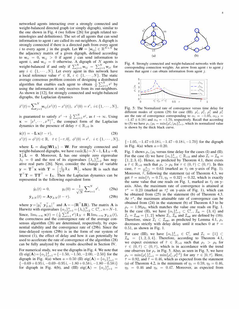
networked agents interacting over a strongly connected andweight-balanced directed graph (or simply digraph), similar tothe one shown in Fig. 4 (we follow [26] for graph related ter-minologies and definitions). The set of all agents that can sendinformation to agent i are called its out-neighbors. A digraph isstrongly connected if there is a directed path from every agenti to every agent j in the graph. Let W = [wij ] ∈ RN×N bethe adjacency matrix of a given digraph, defined accordingto wii = 0, wij > 0 if agent j can send information toagent i, and wij = 0 otherwise. A digraph of N agents isweight-balanced if and only if

∑Nj=1 wij =

∑Nj=1 wji for

any i ∈ {1, · · · , N}. Let every agent in this network havea local reference value ri ∈ R, i ∈ {1, · · · , N}. The staticaverage consensus problem consists of designing a distributedalgorithm that enables each agent to obtain 1

N

∑Nj=1 r

j byusing the information it only receives from its out-neighbors.As shown in [12], for strongly connected and weight-balanceddigraphs, the Laplacian dynamics

xi(t)=∑N

j=1wij(x

j(t)− xi(t)), xi(0) = ri, i∈{1, · · · , N},

is guaranteed to satisfy xi → 1N

∑Nj=1 r

j , as t → ∞. Usingx = [x1, · · · , xN ]>, the compact form of the Laplaciandynamics in the presence of delay τ ∈ R>0 is

x(t) = −Lx(t− τ), (28)xi(t) = φi(t) ∈ R, t ∈ [−τ, 0], φi(0) = ri, i ∈ {1, · · · , N},

where L = diag(W1N ) − W. For strongly connected andweight-balanced digraphs, we have rank(L)=N−1, L1N =0,1>NL = 0. Moreover, L has one simple zero eigenvalueλ1 = 0 and the rest of its eigenvalues {λj}Nj=2 has neg-ative real parts [26]. Next, consider the change of variabley = T>x with T =

[1√N1N R

], where R is such that

T>T = TT> = IN . Then the Laplacian dynamics can berepresented in the following equivalent form

y1(t) = 0, y1(0) =1√N

∑N

i=1ri, (29a)

y2:N (t) = Ay2:N (t− τ). (29b)

where y=[y>1 y>2:N ]> and A=−(R>LR). The matrix A isHurwitz with eigenvalues {αj}nj=1 ={λi}Ni=2 ⊂ Cl−, n=N−1.Since, limt→∞ x(t) = ( 1

N

∑Ni=1 r

i)1N + R limt→∞ y2:N (t),the correctness and the convergence rate of the average con-sensus algorithm (28) are determined, respectively, by expo-nential stability and the convergence rate of (29b). Since thetime-delayed system (29b) is in the form of our system ofinterest (1), the effect of delay and how it can potentially beused to accelerate the rate of convergence of the algorithm (28)can be fully analyzed by the results described in Section IV.For numerical study, we use the digraphs in Fig. 4. We note that(I) eig(A)={αj}4j=1 ={−1.50,−1.50,−2.00,−2.50} for thedigraph in Fig. 4(a) when a= 0.50 (II) eig(A) = {αj}4j=1 ={−0.69+0.95 i,−0.69−0.95 i,−1.80+0.58 i,−1.80−0.58 i}for digraph in Fig. 4(b), and (III) eig(A) = {αj}4j=1 =

Fig. 4: Strongly connected and weight-balanced networks with theircorresponding connection weights. An arrow from agent i to agent jmeans that agent i can obtain information from agent j.

0 0.5 10

1

2

3

4

51/

0

4/0

2,3/0

/0

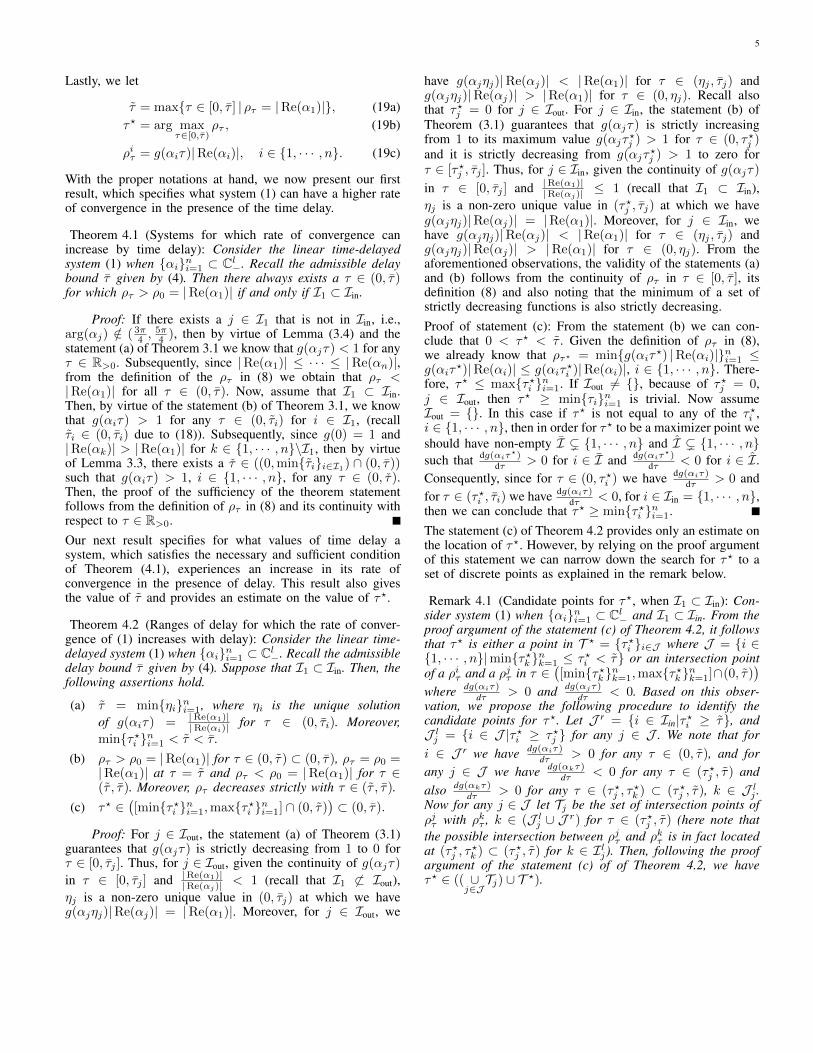
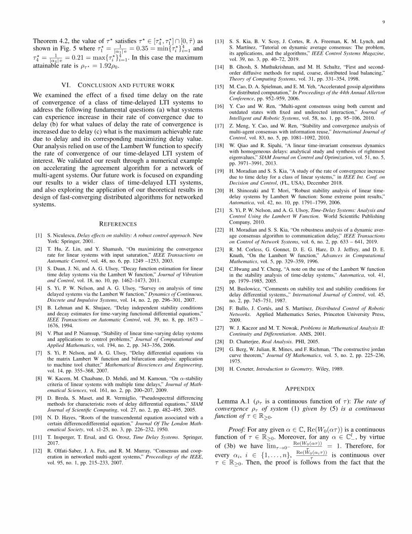
Fig. 5: The Normalized rate of convergence versus time delay fordifferent modes of system (29) for case (III). ρ1τ , ρ2τ , ρ3τ and ρ4τare the rate of convergence corresponding to α1 = −1.05, α2,3 =−1.47± 0.18 i and α4 = −1.70, respectively. Recall that accordingto (5) we have ρτ/ρ0 = min{ρiτ/ρ0}4i=1, which its normalized valueis shown by the thick black curve.

{−1.05,−1.47+0.18 i,−1.47−0.18 i,−1.70} for the digraphin Fig. 4(a) when a=0.20.Fig. 1 shows ρτ/ρ0 versus time delay for the cases (I) and (II).For the case (I) we have {αi}4i=1 ⊂ R<0 and also I1 = Iin ={1, 2, 3, 4}. Hence, as predicted by Theorem 4.1, there existsa τ ∈ R>0 such that ρτ > ρ0 for τ ∈ (0, τ) ⊂ (0, τ). In thiscase, τ = π

2|α4| = 0.63 (marked as τI on y-axis of Fig. 1).Moreover, τ , following the statement (a) of Theorem 4.3, weget τ = min{τ1 = 0.71, η4 = 0.32} = 0.32, which is exactlythe same value that one reads on Fig. 1, marked as τI on y-axis. Also, the maximum rate of convergence is attained atτ? = 0.23 (marked as τ?I on y-axis of Fig. 1), which canbe obtained from (25) in the statement (b) of Theorem 4.3.At τ?, the maximum attainable rate of convergence can beobtained from (24) in the statement (b) of Theorem 4.3 to beρτ = 1.98ρ0, which matches the value one reads on Fig. 1.In the case (II), we have {αi}4i=1 ⊂ Cl−, Iin = {3, 4} andI1 = Iout = {1, 2} where I1, Iin and Iout are defined by (16).Therefore, since I1 ⊂ Iout, as predicted by Lemma 4.1, ρτdecreases strictly with delay delay until it reaches 0 at τ =0.51, as shown in Fig. 1.For case (III), we have {αi}4i=1 ∈ Cl− and I1 = {1} ⊂Iin = {1, 2, 3, 4}. Therefore, according to Theorem 4.1,we expect existence of τ ∈ R>0 such that ρτ > ρ0 forτ ∈ (0, τ) ⊂ (0, τ), which is in accordance with the trendone observes for ρτ in Fig. 5. Also, as seen in Fig. 5, we haveρτ = min{ρiτ}4i=1 = min{ρ1

τ , ρ2,3τ } for any τ ∈ [0, τ ]. Here,

τ = 0.92, and τ = 0.46, which as expected from the statement(a) of Theorem 4.2, is the minimum of η1 = 0.59, η2 = 0.46,η3 = 0.46 and η4 = 0.47. Moreover, as expected from

9

Theorem 4.2, the value of τ? satisfies τ? ∈ [τ?4 , τ?1 ]∩ [0, τ) as

shown in Fig. 5 where τ?1 = 1|α1| e = 0.35 = min{τ?i }4i=1 and

τ?4 = 1|α4| e = 0.21 = max{τ?i }4i=1. In this case the maximum

attainable rate is ρτ? = 1.92ρ0.

VI. CONCLUSION AND FUTURE WORK

We examined the effect of a fixed time delay on the rateof convergence of a class of time-delayed LTI systems toaddress the following fundamental questions (a) what systemscan experience increase in their rate of convergence due todelay (b) for what values of delay the rate of convergence isincreased due to delay (c) what is the maximum achievable ratedue to delay and its corresponding maximizing delay value.Our analysis relied on use of the Lambert W function to specifythe rate of convergence of our time-delayed LTI system ofinterest. We validated our result through a numerical exampleon accelerating the agreement algorithm for a network ofmulti-agent systems. Our future work is focused on expandingour results to a wider class of time-delayed LTI systems,and also exploring the application of our theoretical results indesign of fast-converging distributed algorithms for networkedsystems.

REFERENCES

[1] S. Niculescu, Delay effects on stability: A robust control approach. NewYork: Springer, 2001.

[2] T. Hu, Z. Lin, and Y. Shamash, “On maximizing the convergencerate for linear systems with input saturation,” IEEE Transactions onAutomatic Control, vol. 48, no. 6, pp. 1249 –1253, 2003.

[3] S. Duan, J. Ni, and A. G. Ulsoy, “Decay function estimation for lineartime delay systems via the Lambert W function,” Journal of Vibrationand Control, vol. 18, no. 10, pp. 1462–1473, 2011.

[4] S. Yi, P. W. Nelson, and A. G. Ulsoy, “Survey on analysis of timedelayed systems via the Lambert W function,” Dynamics of Continuous,Discrete and Impulsive Systems, vol. 14, no. 2, pp. 296–301, 2007.

[5] B. Lehman and K. Shujaee, “Delay independent stability conditionsand decay estimates for time-varying functional differential equations,”IEEE Transactions on Automatic Control, vol. 39, no. 8, pp. 1673 –1676, 1994.

[6] V. Phat and P. Niamsup, “Stability of linear time-varying delay systemsand applications to control problems,” Journal of Computational andApplied Mathematics, vol. 194, no. 2, pp. 343–356, 2006.

[7] S. Yi, P. Nelson, and A. G. Ulsoy, “Delay differential equations viathe matrix Lambert W function and bifurcation analysis: applicationto machine tool chatter,” Mathematical Biosciences and Engineering,vol. 14, pp. 355–368, 2007.

[8] W. Kacem, M. Chaabane, D. Mehdi, and M. Kamoun, “On α-stabilitycriteria of linear systems with multiple time delays,” Journal of Math-ematical Sciences, vol. 161, no. 2, pp. 200–207, 2009.

[9] D. Breda, S. Maset, and R. Vermiglio, “Pseudospectral differencingmethods for characteristic roots of delay differential equations,” SIAMJournal of Scientific Computing, vol. 27, no. 2, pp. 482–495, 2005.

[10] N. D. Hayes, “Roots of the transcendental equation associated with acertain differencedifferential equation,” Journal Of The London Math-ematical Society, vol. s1-25, no. 3, pp. 226–232, 1950.

[11] T. Insperger, T. Ersal, and G. Orosz, Time Delay Systems. Springer,2017.

[12] R. Olfati-Saber, J. A. Fax, and R. M. Murray, “Consensus and coop-eration in networked multi-agent systems,” Proceedings of the IEEE,vol. 95, no. 1, pp. 215–233, 2007.

[13] S. S. Kia, B. V. Scoy, J. Cortes, R. A. Freeman, K. M. Lynch, andS. Martınez, “Tutorial on dynamic average consensus: The problem,its applications, and the algorithms,” IEEE Control Systems Magazine,vol. 39, no. 3, pp. 40–72, 2019.

[14] B. Ghosh, S. Muthukrishnan, and M. H. Schultz, “First and second-order diffusive methods for rapid, coarse, distributed load balancing,”Theory of Computing Systems, vol. 31, pp. 331–354, 1998.

[15] M. Cao, D. A. Spielman, and E. M. Yeh, “Accelerated gossip algorithmsfor distributed computation,” In Proceedings of the 44th Annual AllertonConference, pp. 952–959, 2006.

[16] Y. Cao and W. Ren, “Multi-agent consensus using both current andoutdated states with fixed and undirected interaction,” Journal ofIntelligent and Robotic Systems, vol. 58, no. 1, pp. 95–106, 2010.

[17] Z. Meng, Y. Cao, and W. Ren, “Stability and convergence analysis ofmulti-agent consensus with information reuse,” International Journal ofControl, vol. 83, no. 5, pp. 1081–1092, 2010.

[18] W. Qiao and R. Sipahi, “A linear time-invariant consensus dynamicswith homogeneous delays: analytical study and synthesis of rightmosteigenvalues,” SIAM Journal on Control and Optimization, vol. 51, no. 5,pp. 3971–3991, 2013.

[19] H. Moradian and S. S. Kia, “A study of the rate of convergence increasedue to time delay for a class of linear systems,” in IEEE Int. Conf. onDecision and Control, (FL, USA), December 2018.

[20] H. Shinozaki and T. Mori, “Robust stability analysis of linear time-delay systems by Lambert W function: Some extreme point results,”Automatica, vol. 42, no. 10, pp. 1791–1799, 2006.

[21] S. Yi, P. W. Nelson, and A. G. Ulsoy, Time-Delay Systems: Analysis andControl Using the Lambert W Function. World Scientific PublishingCompany, 2010.

[22] H. Moradian and S. S. Kia, “On robustness analysis of a dynamic aver-age consensus algorithm to communication delay,” IEEE Transactionson Control of Network Systems, vol. 6, no. 2, pp. 633 – 641, 2019.

[23] R. M. Corless, G. Gonnet, D. E. G. Hare, D. J. Jeffrey, and D. E.Knuth, “On the Lambert W function,” Advances in ComputationalMathematics, vol. 5, pp. 329–359, 1996.

[24] C.Hwang and Y. Cheng, “A note on the use of the Lambert W functionin the stability analysis of time-delay systems,” Automatica, vol. 41,pp. 1979–1985, 2005.

[25] M. Buslowicz, “Comments on stability test and stability conditions fordelay differential systems,,” International Journal of Control, vol. 45,no. 2, pp. 745–751, 1987.

[26] F. Bullo, J. Cortes, and S. Martınez, Distributed Control of RoboticNetworks. Applied Mathematics Series, Princeton University Press,2009.

[27] W. J. Kaczor and M. T. Nowak, Problems in Mathematical Analysis II:Continuity and Differentiation. AMS, 2001.

[28] D. Chatterjee, Real Analysis. PHI, 2005.[29] G. Berg, W. Julian, R. Mines, and F. Richman, “The constructive jordan

curve theorem,” Journal Of Mathematics, vol. 5, no. 2, pp. 225–236,1975.

[30] H. Coxeter, Introduction to Geometry. Wiley, 1989.

APPENDIX

Lemma A.1 (ρτ is a continuous function of τ ): The rate ofconvergence ρτ of system (1) given by (5) is a continuousfunction of τ ∈ R≥0.

Proof: For any given α ∈ C, Re(W0(ατ)) is a continuousfunction of τ ∈ R≥0. Moreover, for any α ∈ Cl−, by virtueof (3b) we have limτ→0−

Re(W0(ατ))τ = 1. Therefore, for

every αi, i ∈ {1, . . . , n}, Re(W0(αiτ))τ is continuous over

τ ∈ R≥0. Then, the proof is follows from the fact that the

10

maximum/minimum of continuous functions is a continuousfunction (c.f. [27, Problem 1.2.13]).The rest of this appendix contains the proof of the lemmas ofSection III.

Proof of Lemma 3.2: Given the definition of g(x) in (7),the proof of (9a) follows directly from (3b).To validate (9b), we proceed as follows. Note that g(ατ) = 0requires Re(W0(ατ)) = 0 which implies that W0(ατ) = u ifor some non-zero u ∈ (−π, π). Following the definition ofthe Lambert W function, then, we can write

u eui = (Re(α)τ + i Im(α)τ)⇔{−u sin(u) = Re(α)τ,

u cos(u) = Im(α)τ,

⇔

{u2 = τ2|α|2,tan(u) = Re(α)

Im(α) ,

which for u ∈ (−π, π), after eliminating u gives τ =

|atan(Re(α)Im(α) )|

/|α| as the unique solution for g(ατ) = 0. For

α ∈ R<0, we have atan(Re(α)Im(α) ) = π

2 , which means thatτ = π

2|α| . Finally, to validate (10) we proceed as follows.g(ατ) = 1 means that Re(W0(ατ)) = Re(ατ). Then,W0(ατ) = Re(ατ) + i θ for some non-zero θ ∈ (−π, π).Then, we obtain the value of θ as follows. Invoking definitionof Lambert function, we have

(Re(ατ) + θ i) eRe(ατ)+θ i = Re(ατ),

⇔{θ cos θ + Re(ατ) sin θ = 0,

eRe(ατ)(

Re(ατ) cos θ − θ sin θ)

= Re(ατ),

which using some trigonometric manipulations can also bestated equivalently as

Re(ατ) = −θ cot(θ) (A.1a)

e−θ cot(θ) = cos(θ). (A.1b)

For θ ∈ (−π, π), (A.1b) has two distinct solutions θ ≈±1.01125. Thus, the proof of (10) follows from (A.1a).To prove the rest of the results in Section III we rely onstudying the derivative of g(x) along x = ατ with respect toτ ∈ R>0 for a given α ∈ C. Using (3a) and (7), the derivativeof delay rate gain function along x = ατ 6= − 1

e with respectto time delay τ ∈ R>0 can be written as

d g(ατ)

dτ=

1

Re(α)

[− 1

τ2Re(W0(ατ))+

1

τRe(

α

ατ+eW0(ατ))],

which can also be represented as

d g(ατ)

dτ= − 1

Re(α)τ2Re(

ατ W0(ατ)

ατ + eW0(ατ))

= − 1

Re(α)τ2Re(

W 20 (ατ)

1 +W0(ατ)).

Let W0(ατ) = w + i u, where u ∈ (−π, π). Then, for x =ατ 6= − 1

e , we can write

d g(ατ)

dτ=− 1

Re(α)τ2

w3 + w2 − u2 + wu2

(w + 1)2 + u2

=− 1

Re(α)τ2

(w2 + u2)w + (w2 − u2)

(w + 1)2 + u2. (A.2)

At ατ =− 1e , the right and the left derivative of g(ατ) along

x = ατ are obtained as follows. For x = ατ ∈ [− 1e , 0],

W0(x)∈R. Thus, by setting u = 0, (A.2) gives

d g(ατ)

dτ=

1

|α| τ2

w2

(w + 1), τ ∈ (0,

1

e |α|), (A.3)

thus

limτ→ 1

e |α|−

d g(α τ)

dτ= lim

w→−1+e2 |α| w2

(w + 1)= +∞. (A.4)

For any x = ατ ∈ (−∞,− 1e ), W0(x) = w + i u is a complex

number with u ∈ (0, π), and satisfies

(w + i u) ew+u i = ατ ⇔{

ew (w cos(u)− u sin(u)) = ατ,

ew (u cos(u) + w sin(u)) = 0.

Therefore, for ατ ∈ (−∞,− 1e ), for which we always have

u 6= 0, we have w = −u cos(u)/ sin(u) and

d g(α τ)

dτ=

1

|α| τ2

u2(−u cos(u)sin(u) + cos(2 u))

(−u cos(u)+sin(u))2 + u2 sin2(u).

(A.5)

Using the L’Hospital’s rule [28, Theorem 5.5.2], we can thencolcude that

limτ→ 1

e |α|+

d g(α τ)

dτ= (A.6)

e2 |α| limu→0

u2

sin2(u)(−u cos(u)

sin(u) + cos(2u))

(−u cos(u)sin(u) + 1)2 + u2

= −5 e2 |α|3

.

Next is an intermediate result that we use in the proofLemma 3.4 and Lemma 3.6. To establish this result, we relyon the Jordan Curve Theorem, which states that a simpleand closed curve divides the plane into an “interior” regionbounded by the curve and an “exterior” region containing allof the nearby and far away exterior points [29].

Lemma A.2 (Some of the properties of level set C0 and super-level set S0): Consider the level set C0 (11a) and the superlevelset S0 (11b). Let C0 = C0 ∪ {(0, 0)} and S0 = S0 ∪ {(0, 0)}.Then, the following assertions hold.

(a) C0 is a simple closed curve in R2 that is symmetric aboutthe x axis and intersects the x axis at only two pointsx = 0 and x = −π2 . Moreover, it passes through theorigin tangent to the y axis.

(b) S0 = C0 ∪ int(C0), and is a compact convex subset ofR2.

11

(c) Cc ⊂ int(C0) ⊂ S0 for c > 0 and Cc ⊂ ext(C0) forc < 0.

Proof: For a c ∈ R, by definition, g(x) = c for anyx = (x + y i) ∈ Cl− is equivalent to Re(W0(x + yi)) = c x.In other words, W0(x + y i) = c x + u i, where u ∈ (−π, π).Thereby, given property (2e) of the Lambert W0 function, eachlevel set Cc, c ∈ R, is symmetric about the real axis. Moreover,from the definition of the Lambert W function we can write

(c x + u i) ec x+ui = x + yi⇔{

ec x (c x cos(u)− u sin(u)) = x,

ec x (u cos(u) + c x sin(u)) = y.(A.7)

For c = 0, by eliminating u in (A.7) via trigonometricmanipulations, we can characterize C0 by

C0 ={

(x, y) ∈ R<0×R∣∣∣ xy

= ± tan(√

x2+y2),

0 < (x2+y2) < π2}.

In polar coordinates, any (x, y) ∈ C0, reads as x = r cos(θ)and y = r sin(θ) with{

tan(r) = ± cot(θ), θ ∈ (π2 ,3π2 ),

0 < r < π,

Therefore, C0 ={

(x, y) ∈ R<0 ×R∣∣∣ x = r cos(θ), y =

±r sin(θ), r = θ − π2 , θ ∈ (π/2, π]

}. Evidently,

C0 ={

(x, y) ∈ R≤0×R∣∣∣ x = r cos(θ), y = ±r sin(θ),

r = θ − π

2, θ ∈ [π/2, π]

}. (A.9)

From (A.9), for any point on the upper half (resp. positive y)and lower half (resp. negative y) of C0, in polar coordinates,r is a continuous and a bounded function of θ and d r

d θ = 1exists on θ ∈ (π/2, π) (resp. θ ∈ (π, 3π/2)). Therefore, C0is a simple closed curve. Next, note that on C0, as θ → π+

2 ,and due to symmetry also as θ → 3π−

2 , it follows that r → 0.Therefore, C0 passes through the origin tangent to the y axis.Also, at θ = π

2 and θ = π we have, respectively, (x, y) = (0, 0)and (x, y) = (−π2 , 0). As a result, assertion (a) holds.

Since C0 is a simple closed curve, it follows from the JordanCurve Theorem that C0 divides the plane into an interiorregion bounded by C0 and an exterior region containing allof the nearby and far away exterior points. Moreover, notethat the curvature of the upper half of C0 in a (x, y) plane isκ =

r2+2r2θ−rrθθ(r2+r2θ)

32

= r2+2

(r2+1)32> 0, where (.)θ = ∂(.)/∂θ [30].

Therefore the upper half curve of C0 is a convex curve.Consequently, Z = C0∪int(C0) is a compact convex set (recallthat C0 is symmetric about x axis). To complete the proof ofthe statement (b), we show that S0 = Z .Consider an α ∈ Cl− and recall τ in (9b). Because(0, 0) ∈ bd(Z) and (Re(ατ), Im(ατ)) ∈ bd(Z) (recallg(ατ) = 0), it follows from the compact convexity ofZ that (Re(ατ), Im(ατ)) ∈ int(C0) for τ ∈ (0, τ) and

(Re(ατ), Im(ατ)) ∈ ext(C0) for τ ∈ (τ ,∞). Therefore,given that g(ατ) is a continuous function of τ ∈ R≥0 (seeLemma 3.3) and g(ατ) at τ = 0 and τ = τ is equal to,respectively, 1 and 0, we can conclude that g(ατ) > 0 forany τ ∈ (0, τ). This means that at any (Re(ατ), Im(ατ)) ∈int(C0), we have g(ατ) > 0. Consequently, Z = S0, whichcompletes the proof of statement (b).From validity of the statement (b), we can readily deduce thatCc ⊂ int(C0) ⊂ S0 for c > 0. To complete the proof of thestatement (c), we recall from the proof of the statement (b) thatfor any α ∈ Cl−, (Re(ατ), Im(ατ)) ∈ ext(C0) for τ ∈ (τ ,∞),i.e., g(ατ) 6= 0 for τ ∈ (τ ,∞). Then, combined with the factthat g(ατ) is a continuous function of τ ∈ R≥0 and also thatat τ from (A.2) we have (recall that Re(α) < 0)

dg(ατ)

dτ=

1

Re(α)τ2

u2

1 + u2< 0, (A.10)

we can conclude that g(ατ) < 0 for τ ∈ (τ ,∞). This meansthat Cc ⊂ ext(C0) for c < 0. To arrive at (A.10), we relied onthe knowledge that g(ατ) = 0 indicates that Re(W0(ατ)) = 0,therefore W0(ατ) = 0 + u i for some u ∈ (−π, π).The topological properties of the the C0 level set, which areestablished in Lemma A.2 is evident in Fig. (2). Using theresults of Lemma A.2, we proceed next to present the proofof Lemma 3.4.

Proof of Lemma 3.4: Recall from the statement (b) ofLemma A.2 that S0 is a compact convex set. Therefore, since(Re(ατ), Im(ατ)) ∈ bd(S0) (recall g(ατ) = 0) and (0, 0) ∈bd(S0), then (Re(ατ), Im(ατ)) ∈ int(C0) for τ ∈ (0, τ) and(Re(ατ), Im(ατ)) ∈ ext(C0) for τ ∈ (τ ,∞). Then, the prooffollows from the statement (c) of Lemma A.2.The proof of Lemma 3.4 can also be deduced from thecontinuity stability property theorem [1, Proposition 3.1] forlinear delayed systems. In this regard, consider the dynamicalsystem x =

[Re(α) Im(α)− Im(α) Re(α)

]x(t−τ), whose eigenvalues are α

and conj(α). The real part of the RMR of the CE of this systemis given by Re(Srτ ) = g(ατ) Re(α) (recall (7)). It follows fromthe continuity stability property theorem [1, Proposition 3.1]and Lemma 3.1 that Re(srτ ) ∈ R<0 if and only τ ∈ [0, τ).Therefore, g(ατ) > 0 if and only if τ ∈ [0, τ), which alongwith the fact g(ατ) = 0 validates the statement of Lemma 3.4.Next, we prove Lemma 3.5.

Proof of Lemma 3.5: At τ? = 1/(e |α|),because W0(− e−1) = −1, we have g(ατ?) =Re(W0(− e−1))/(− e−1) = e. Next, note thatfrom (9a), (9b) and Lemma 3.3, we know, respectively,that limτ→0 g(α τ) = 1, τ = τ is the unique solution ofg(ατ) = 0 for τ ∈ R>0, and g(ατ) is a continuous functionof τ ∈ R>0. Therefore, to complete the proof of statement (a),we show next that d g(x)

dτ > 0 for τ ∈ (0, τ?) and d g(x)dτ < 0

for τ ∈ (τ?, τ). For x = ατ ∈ [− 1e , 0], we have W0(x) ∈ R,

and as such by setting u = 0 from (A.2) we obtain

d g(ατ)

dτ=

1

|α| τ2

w2

(w + 1)> 0, τ ∈ (0, τ?). (A.11)

12

Moreover, from (A.4) we have

limτ→τ?−

d g(α τ)

dτ= +∞. (A.12)

For any x = ατ ∈ (−∞,− 1e ), recall that d g(α τ)

dτ is givenby (A.6). Because for ατ ∈ [−π2 ,− 1

e ) we have u ∈ (0, π2 ], wecan confirm that (−u cos(u)

sin(u) + cos(2 u)) < 0 and therefore, weobtain

d g(α τ)

dτ< 0, τ ∈ (τ?, τ ]. (A.13)

Next, note that from (A.6) we have

limτ→τ?+

d g(α τ)

dτ= −5 e2 |α|

3< 0. (A.14)

In light of the observations above, the proof of the statement(b) follows from (9a), (10), (A.11), (A.13) and the continuityof g(ατ) for τ ∈ R>0. Finally, statement (c) is deduced fromstatements (a) and (b), along with (A.12) and (A.14). Note thatsince g(ατ?) = e > 1, we have τ? ∈ [0, τ).

Next, we use the results of Lemma A.2 to establish the proof ofLemma 3.6, which characterizes the variation of d g(x)

dτ alongx = ατ for τ ∈ R>0 such that (Re(x), Im(x)) ∈ S0.

Proof of Lemma 3.6: By virtue of Lemma (3.4), weknow that g(ατ) > 0 for τ ∈ (0, τ), and g(ατ) = 0.Then, it follows from the definition of delay rate gain andRe(α) < 0 that Re(W0(ατ)) < 0 for τ ∈ (0, τ). Conse-quently, for τ ∈ (0, τ ], we have (Re(ατ), Im(ατ)) ∈ S0 and(Re(W0(ατ)), Im(W0(ατ)) ∈ R≤0 × (−π, π).Next, recall that the derivative of g(x) with respect to τ alongx = ατ , except at x = − 1

e , is given by (A.2), where wedenoted W0(ατ) = w+u i, which satisfies u ∈ (−π, π). SinceRe(α) < 0, it is perceived from (A.2) that the sign of d g(x)

dτalong x = ατ is defined solely by the sign of ψ = (w2 +u2)w + (w2 − u2), the nominator of (A.2).Using the polar coordinates and a set of simple trigonometricmanipulations, we identity the points (w, u) ∈ R≤0 × (−π, π)for which ψ retains a zero, a positive and a negative value, as,respectively, Γ, Γ+ and Γ−, where

Γ ={

(w, u) ∈ R≤0 × (−π, π)∣∣w = R cos(θ), u = R sin(θ),

3π/4 ≤ θ ≤ 5π/4 , R = − cos(2θ)/ cos(θ)},

Γ+ ={

(w, u) ∈ R≤0 × (−π, π)∣∣w = R cos(θ), u = R sin(θ),

3π/4 ≤ θ ≤ 5π/4 , R < − cos(2θ)/ cos(θ)},

Γ− = (R≤0 × (−π, π)) \(Γ ∪ Γ+).

Therefore, for x = ατ with τ ∈ (0, τ ] we have

d g(x)

dτ> 0 if (Re(W0(x)), Im(W0(x))) ∈ Γ+,

d g(x)

dτ= 0 if (Re(W0(x)), Im(W0(x))) ∈ (Γ\{(−1, 0)}),

d g(x)

dτ< 0 if (Re(W0(x)), Im(W0(x))) ∈ Γ−.

Here we used W0(− 1e ) = −1.

Now, let ατ = r eφ i and W0(ατ) = R eθ i = R cos(θ) +R sin(θ) i, in which −π < R sin(θ) < π by definition. Then,using the relation W0(ατ) eW0(ατ) = ατ we obtain that

r = R eR cos(θ),

φ = θ + R sin(θ).

Then, recalling the definition of Γ, Γ+ and Γ−, the proof ofpart (a) follows from the observation that for x = ατ , τ ∈(0, τ ] we have

(Re(ατ), Im(ατ)) ∈ int(Λ) ⇒ (w, u) ∈ Γ+,

(Re(ατ), Im(ατ)) ∈ Λ ⇒ (w, u) ∈ Γ ,

(Re(ατ), Im(ατ)) ∈ (S0\(int(Λ) ∪ Λ)) ⇒ (w, u) ∈ Γ−,

where (w, u) = (Re(W0(ατ)), Im(W0(ατ))). Recall here thatW0 function is injective.To prove statement (b) and (c) we proceed as follows. We notethat in (12) r and φ both are a differentiable and a boundedfunction of θ ∈ [ 3π

4 ,5π4 ]. Moreover,

dφd θ

=1 + 2 tan(θ) e− cos 2θ sin(2θ) (1− cos(2θ))−

cos(2θ) e− cos(2θ) (1 + tan2(θ)) > 0, (A.15)

for any θ ∈ [ 3π4 ,

5π4 ]. Therefore, φ in (12) has a one-to-

one correspondence with θ ∈ [ 3π4 ,

5π4 ], which in turn indi-

cates that r in (12) has a one-to-one correspondence withφ. Moreover, since φ( 3π

4 ) = 3π4 and φ( 5π

4 ) = 5π4 , we

have φ ∈ [ 3π4 ,

5π4 ]. In addition, we can also conclude that

drdφ = dr

dθ/dφdθ exists and is finite at every θ ∈ [ 3π

4 ,5π4 ].

Combined with r satisfying r( 3π4 ) = r( 5π

4 ) = 0, we canthen conclude that Λ is a simple closed curve. Therefore, itfollows from the Jordan Curve theorem that int(Λ) ∪ Λ is aconnected compact subset of R2. In light of the precedingobservations, we make the following conclusions. The ray(Re(ατ), Im(ατ)), τ ∈ (0, τ ], intersects Λ if and only if3π4 < arg(α) < 5π

4 . Therefore, if arg(α) 6∈ ( 3π4 ,

5π4 ), we have

(Re(ατ), Im(ατ)) ∈ (S0\(int(Λ)∪Λ)) for τ ∈ (0, τ ]). Then,the proof of the statement (b) follows from the statement (a).On the other hand, if arg(α) ∈ ( 3π

4 ,5π4 ), then due to the one-to-

one correspondence between r and φ, ray (Re(ατ), Im(ατ)),τ ∈ (0, τ ] intersects Λ at a unique point. Let this pointcorrespond to τ? ∈ (0, τ ], i.e., (Re(ατ?), Im(ατ?)) ∈ Λ.Then, (13) is deduced from the definition of Λ in (12). Next,note that from compactness of int(Λ) ∪ Λ) and the fact that(Re(ατ), Im(ατ)), τ ∈ (0, τ ], intersects Λ at a unique point,it follows that (Re(ατ), Im(ατ)) ∈ int(Λ) for τ ∈ (0, τ?) and(Re(ατ), Im(ατ)) ∈ (S0\(int(Λ)∪Λ)). Thereby, by virtue ofthe statement (a) we conclude that dg(ατ)

dτ > 0 for τ ∈ (0, τ?),and dg(ατ)

dτ < 0 τ ∈ (τ?, τ ]. If α ∈ R<0, then arg(α) = π.Therefore, τ? in (13) becomes equal to 1

e |α| , and consequently,(15) follows from (A.4) and (A.6). Lastly, when α 6∈ R<0,

13

since (Re(ατ?), Im(ατ?)) ∈ Λ\{(− 1e , 0)}, dg(ατ)

dτ = 0 atτ = τ? is deduced from the statement (a).Figure 3 depicts Λ in (12) (red curve) in a (x, y) plane alongwith the level sets C1 (green curve) and C0 (blue curve). As onecan expect (given (9) and the statement (a) of Lemma 3.6), Λ islocated inside C1 and between the lines y = ±x. It is interestingto note that lines y = ±x are also tangent to C1 at theorigin. This observation can be verified as follows. Consider(x1, y1) ∈ C1 and let x1 + y1 i = r eiθ. Then, for (x1, y1) inthe close neighborhood of the origin from (9a)) we expectthat limr→0− cos(2 θ) + 3

2 r cos(3 θ)− 83 r

2 cos(4 θ) + · · · = 0.This limit is possible only if θ → 3π

4 and θ → 5π4 (solution

of cos(2 θ) = 0 for θ ∈ [π/2, 3π/2]). This verifies that as(x1 +y1 i)→ 0 on C1, C1 become tangent to the lines y = ±x.