1 pde methods are not necessarily level set methods allen tannenbaum georgia institute of technology...
TRANSCRIPT

1
PDE Methods are Not Necessarily
Level Set Methods
Allen TannenbaumGeorgia Institute of Technology
Emory University
2
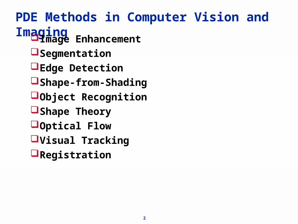
PDE Methods in Computer Vision and ImagingImage Enhancement
Segmentation Edge DetectionShape-from-ShadingObject RecognitionShape TheoryOptical FlowVisual TrackingRegistration
3
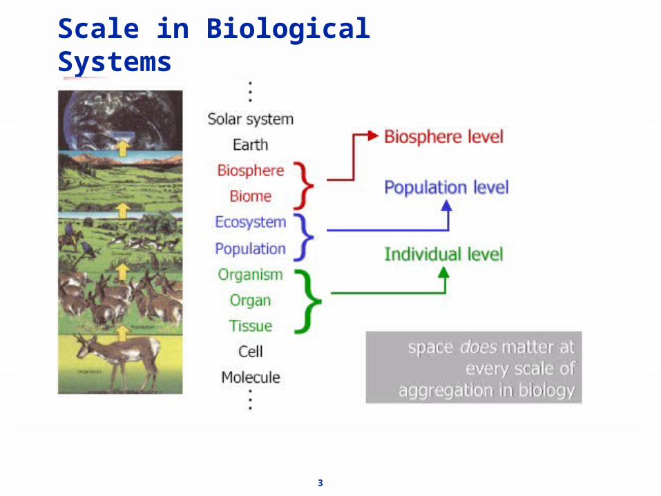
Scale in Biological Systems

4
Micro/Macro Models-Scale I

5
Micro/Macro Models-Scale II

6
How to Move Curves and Surfaces
Parameterized Objects: methods dominate control and visual tracking; ideal for filtering and state space techniques.
Level Sets: implicitly defined curves and surfaces. Several compromises; narrow banding, fast marching.
Minimize Directly Energy Functional: conjugate gradient on triangulated surface (Ken Brakke).

7
Level Sets-A History
Independently: Peter Olver (1976), Ph.D. thesisSigurd Angenent (Leiden University Report, 1982)
Mathematical Justification: Chen-Giga-Goto (1991)Evans and Spruck (1991)

8
When Do They Work

9
Parameterized Curve Description
infinite dimensional
parameterization for derivations only, evolution should be geometric

10
Generic Curve Evolution
The closed curve C evolves according to
moves “particles” along the curve
influences the curve’s shape
How is the speed determined?

11
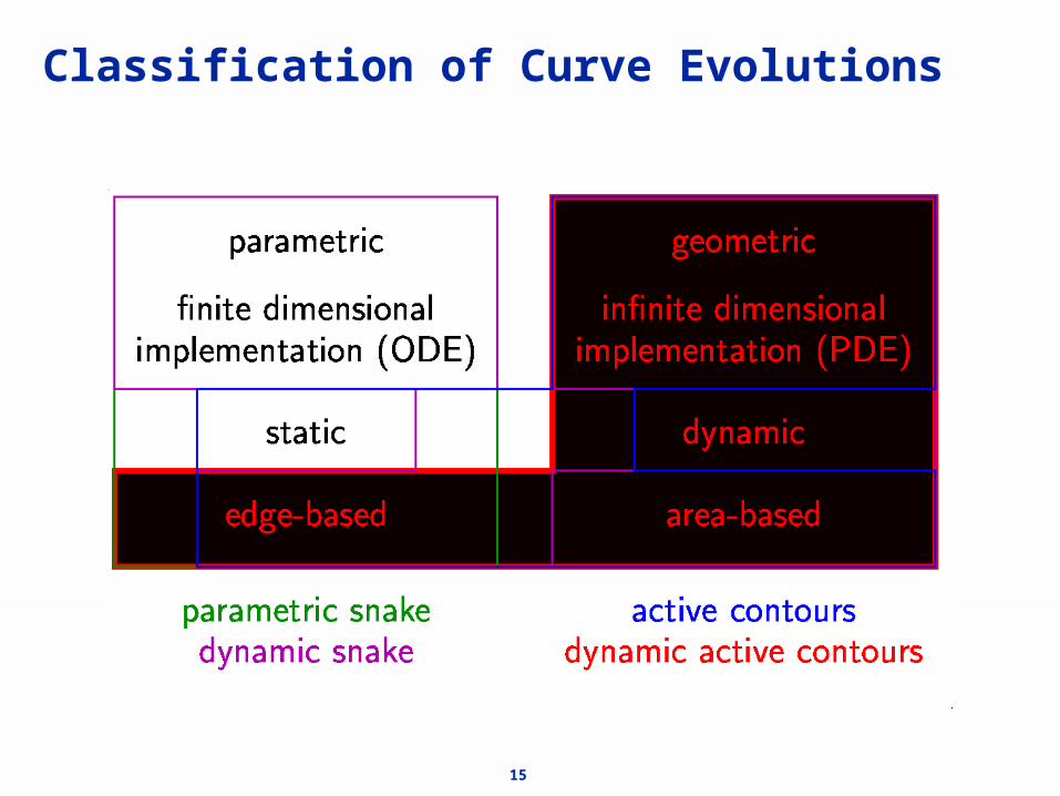
Classification of Curve Evolutions

12
Classification of Curve Evolutions
Kass, Witkin, Terzopoulos, "Snakes: Active Contour Models," International Journal of Computer Vision, pp. 321-331, 1988.

13
Classification of Curve Evolutions
Terzopoulos, Szeliski, Active Vision, chapter Tracking with Kalman Snakes, pp. 3-20, MIT Press, 1992.

14
Classification of Curve Evolutions
Kichenassamy, Kumar, Olver, Tannenbaum, Yezzi, "Conformal curvature flows: From phase transitions to active vision,"Archive for Rational Mechanics and Analysis, vol. 134, no. 3, pp. 275-301, 1996.
Caselles, Kimmel, Sapiro, "Geodesic active contours," International Journal of Computer Vision, vol. 22, no. 1, pp. 61-79, 1997.
15
Classification of Curve Evolutions

16
Static Approaches
Kass snake (parametric)
Geodesic active contour (geometric)
using the functionals
Minimize

17
leads to the Euler-Lagrange equations
Minimizing
Static Approaches
Kass snake (parametric)
Geodesic active contour (geometric)
18
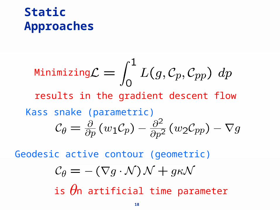
Static Approaches
Kass snake (parametric)
Geodesic active contour (geometric)
results in the gradient descent flow
Minimizing
is an artificial time parameter

19
Dynamic Approach
Minimizethe actionintegral
where is the Lagrangian,
is the kinetic energy and is the potential energy.

20
Dynamic Approach
using the functional
Minimizing
Terzopoulos and Szeliski (parametric)

21
results in the Euler-Lagrange equation
Terzopoulos and Szeliski (parametric)
Minimizing
Dynamic Approach
Here, is physical time

22
Dynamic Approach
But what about a geometric formulation?
results in the Euler-Lagrange equation
Terzopoulos and Szeliski (parametric)
Minimizing

23
Geometric Dynamic Approach
Minimize
using the Lagrangian
results in the Euler-Lagrange equation

24
Geometric Dynamic Approach
We can write
We then obtain the following two coupled PDEs for the tangential and the normal velocities:
The tangential velocity matters.

25
PDE’s Without Level Sets: Some Examples
26
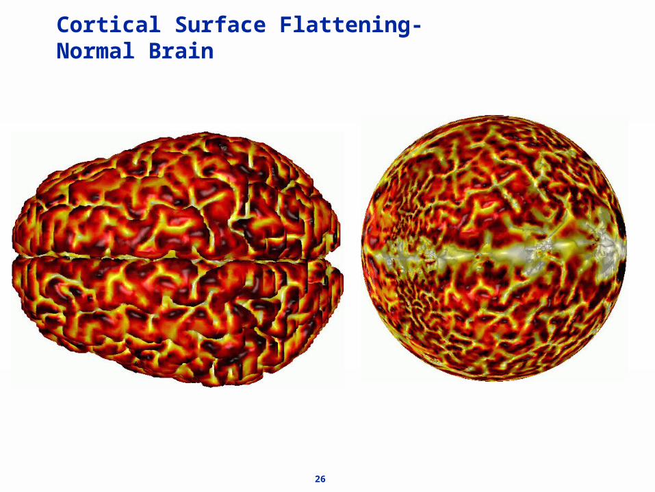
Cortical Surface Flattening-Normal Brain
27
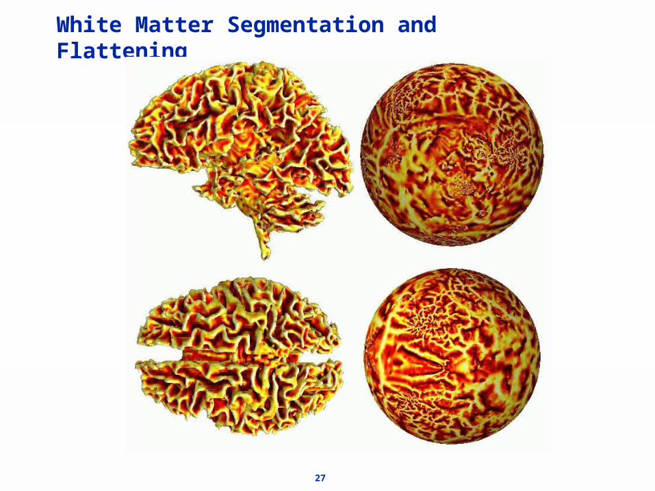
White Matter Segmentation and Flattening

28
Conformal Mapping of Neonate Cortex

29
Surface Warping-Area Preserving
30
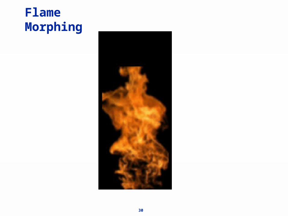
Flame Morphing

31
Anisotropic active contours
• Add directionality
32
Curve minimization
Calculus of variationsStart with initial curveDeform to minimize energySteady state is locally optimum
Dynamic programmingChoose seed point sFor any point t, determine globally
optimal curve t s
Registration,Atlas-basedsegmentation
Segmentation

33
Synthetic example (3D)

34
Stochastic Approximations

35
Curvature Driven Flows

36
Euclidean and Affine Flows
37
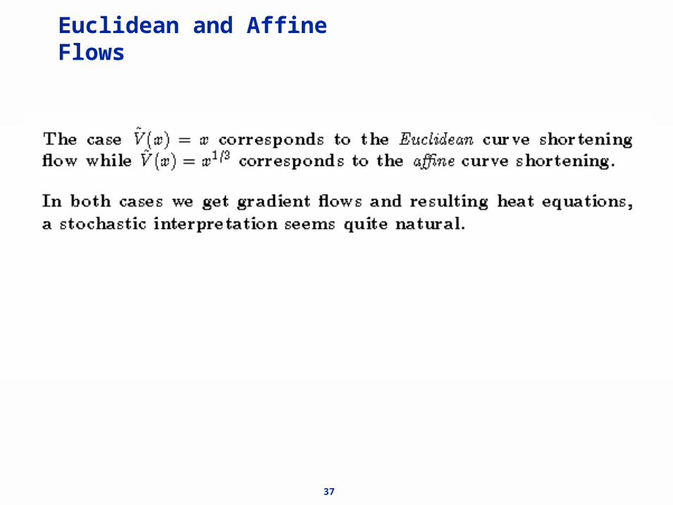
Euclidean and Affine Flows

38
Birth/Death Zero Range Processes-I
S: discrete torus TN, W=N
Particle configuration space: N TN
Markov generator:
)()()( 12 fLfLNLf o

39
Birth/Death Zero Range Processes-II
Markov generator:
)()()( 12 fLfLNLf o
)](2)()())[((2
1)( 1,1,
0 fffigfL ii
Ti
ii
N
elsej
iijj
iijj
jii
),(
0)(,,1)(
0)(,11)(
)(1,
40
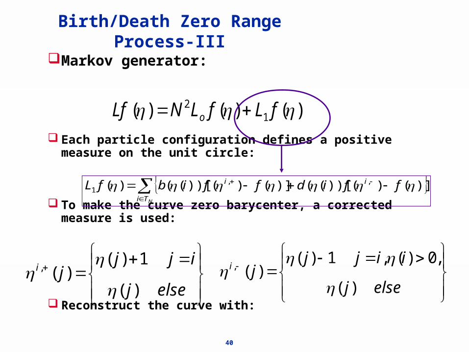
Birth/Death Zero Range Process-III
Markov generator:
Each particle configuration defines a positive measure on the unit circle:
To make the curve zero barycenter, a corrected measure is used:
Reconstruct the curve with:
)()()( 12 fLfLNLf o
NTi
ii ffidffibfL )]()())[(()]()())[(()( ,,1
elsej
ijjji
)(
1)()(,
elsej
iijjji
)(
,0)(,1)()(,

41
The Tangential Component is Important

42
Nonconvex Curves

43
Stochastic Interpretation-I

44
Stochastic Interpretation-II

45
Stochastic Interpretation-III

46
Stochastic Curve Shortening

47
ConclusionsLevel sets are a way of implementing
curvature driven flows.
Loss of information.
Modifications are necessary.
Do not work if no maximum principle.
Combination with other methods, e.g. Bayesian.