University of Saskatchewan, Electrical EngineeringEE 480.3 Digital Control

Review of Analog Controller DesignJanuary, 2003 by K. Takaya

1 Planar Robot Arm

Consider one of the arms in a multi-joint robot manipulator to illustratethe design process of controllers (compensators). The arms of a practi-cal robot manipulator is affected by the gravitational field due to the massof each arm. This makes even such a simple mechanical rotational sys-tem nonlinear and analysis difficult. Though negative feedback works evenfor nonlinear systems, we assume the particular arm under discussion isplaced horizontally without being affected by the gravitational field. We re-fer this type of robot arms to as planar robot arms. There are three majorcomponents necessary to drive such a robot arm. One is a servo-motorbuilt inside the joint. We need a power supply to drive the servomotor. Thearm itself is a mechanical component. The specification sheets indicatemajor parameters necessary to describe the overall system which will bethen used to design a controller.

Fig. 1 Schematic Diagram of a Planar Robot Arm

The specifications of the servo-motor (embedded direct drive DC mo-tor) are:

1

1. General: High initial torque, linear torque DC motor2. Input Voltage: ±28V maximum3. Output Torque: not specified4. Angular Velocity: 3,600 rpm at 24V5. Output Power: 1/20 HP at 24V6. Torque Linearity: less than 1% within ±28V7. Input Current: 4A at 24V

The power supply to be used is a voltage source for which the outputvoltage is controlled by the input voltage.

1. Maximum Current: 5A2. Input Voltage: ±28V3. Voltage Gain: unity4. Input Impedance: 100KΩ5. Settling Time: 10ms for 24V

The mechanical specifications are known only in terms of the time con-stant associated with each arm. The particular arm of interest is quotedas 2 seconds.

2 System Description

The basic equation describing the dynamics of the arm is a second orderdifferential equation,

Jθ + f θ = τ

where J is the inertia of the arm, f is the friction coefficient, θ is the angleof rotation, and τ is the applied torque. From this differential equation, thetransfer function can be derived as

G0(s) =θ(s)

T(s)=

1s(Js + f )

=1/f

s(Jf s + 1)

Since J/f = T , mechanical time constant, and the torque is a linear func-tion of the input voltage Ea, i.e. τ = AEa, the transfer function from theinput voltage Ea to the angle θ now becomes,

G(s) =θ(s)

Ea(s)=

Af

s(Jf s + 1)=

Ks(T s + 1)

.

2

The transfer function from the input voltage Ea to the angular velocity ofthe arm ω is also given by

Gω(s) =Ω(s)

Ea(s)=

KTs + 1

.

If this arm is vertically placed instead of horizontally, the arm is affectedby the gravitational field. In this case, the system’s equation needs tobe modified by taking an additional torque into account. Assuming thedistance from the pivot (centre of arm rotation) to the centre of the gravitybeing equal to ` , the differential equation is,

Jθ + f θ = τ +Mg` cos(θ).

Since this equation involves θ, θ and cos(θ) in a differential equation, thissystem is no longer linear.

From the given specifications, we know that the motor rotates at 3,600rpm when the input voltage is 12V. However, this motor has a built-in gear(down-gear) of 60:1 in its gear ratio. The speed of rotation at the outputshaft is, therefore, 60 rpm which is 1 rps (revolutions per second or cy-cles/s). We decide here to use rps (cycles/s) in our system model. Usingthe final value theorem of the Laplace transform, we now determine twoimportant parameters, the gain K and time constant T .

Ωss = lims→0

sK

Ts + 1· 24s

= 24K = 1rps

Thus, K = 1/24. Time constant T is given as 2 seconds. To check theefficiency of the robot arm, calculate the input and output power. The inputpower is 24V×4A=96 watts. The output power at the input voltage of 24Vis 1/20 HP, which is 1

20 × 746 = 37.3 watts. The efficiency is calculated tobe 0.3885.

3 Open-Loop Control

This particular one arm of the robot manipulator can do angular positioningwithout negative feedback. By simply applying a fixed voltage for a certain

3

time period, the arm rotates and come to a desired position. This is open-loop control. Let us determine how long a voltage of 24V has to be appliedto change the arm position by 90 or 1/4 of a revolution. This on-off controlis described by

θ(s) =1/24

s(2s + 1)· V0(

1s− e

−sT

s),

where V0 is the input voltage and and T is the duration of time that V0 isapplied.

L−1 V0

241

s2(2s + 1)=V0

48(2t − 4 + 4e−0.5t)

yields

θ(t) =V0

48(2t − 4u(t) + 4e−0.5t) − (2(t − T ) − 4u(t − T ) + 4e−0.5(t−T )).

Thus, the final value at t =∞ is

limt→∞

θ(t) =V0

48(2T ) =

14

revolutions

If we apply V0 = 24V, T is, therefore, 0.25 seconds. Remember this value,to turn the arm 90 the required time is 0.25 seconds at 24V.

4 Closed-Loop Control

The same task as considered previously as open-loop control can be ac-complished by closed-loop control that provides negative feedback. Theopen-loop control cannot correct the set position of 90 in the event that theangle is disturbed. Whereas, the feedback has ability to detect the errorcaused by the disturbance and correct the error. This added functional-ity is achieved at the expense of response time as well as higher powerrequirements. We will investigate how the performance of the system isaltered by the closed loop configuration with a negative feedback loop.

We need to use a position sensor to detect the angular position of therobot arm. The simplest position detector is a potentiometer. We supply±12V between two end terminals and measure the voltage of the brush

4

relative to the ground. Since one revolution gives a voltage change of 24V,the sensor gain is 24V/revolution. The transfer function is

Ep(s) = 24θ(s).

Fig. 2 Block diagram of the closed loop system

Incorporating two potentiometers, one to set a reference angle and theother to measure the output angular position, the block diagram of theclosed-loop control system is illustrated in Fig. 2. After simplification, weobtain the block diagram as shown at the bottom of Fig. 2.

We now examine the characteristics of the closed-loop system in termsof the commonly used indices such as damping ratio, time constant, set-tling time, phase margin etc. According to Fig. 2, the open-loop (forward)transfer function is

G(s) =0.5

s(s + 0.5).

The feedback transfer function is H(s) = 1. The closed-loop transfer func-tion is given by

Gc(s) =G(s)

1 + G(s)H(s)=

0.5s2 + 0.5s + 0.5

.

5

From the characteristic equation s2+0.5s+0.5 = 0, the roots representingthe closed-loop poles are found to be

s = −14± j√

74

= −0.25 ± j0.6614.

The root locus plot for the open-loop transfer function G(s) varying the loopgain can be plotted easily with a Matlab statement, rlocus([0.5],[1, 0.5, 0]);

The calculated poles can be verified in the root locus plot. The loop gainis unity in this case.

Fig. 3 The root locus plot for G(s)

Referring to the standard 2nd order transfer function,

G2(s) =ω2n

s2 + 2ζωns +ω2n

,

the poles of this system are located at

s = −ζωn ± jωn√

1 − ζ2.

This equation defines damping ratio ζ and damped natural frequency ωdas

ζ = cosθ and ωd = ωn

√

1 − ζ2.

6

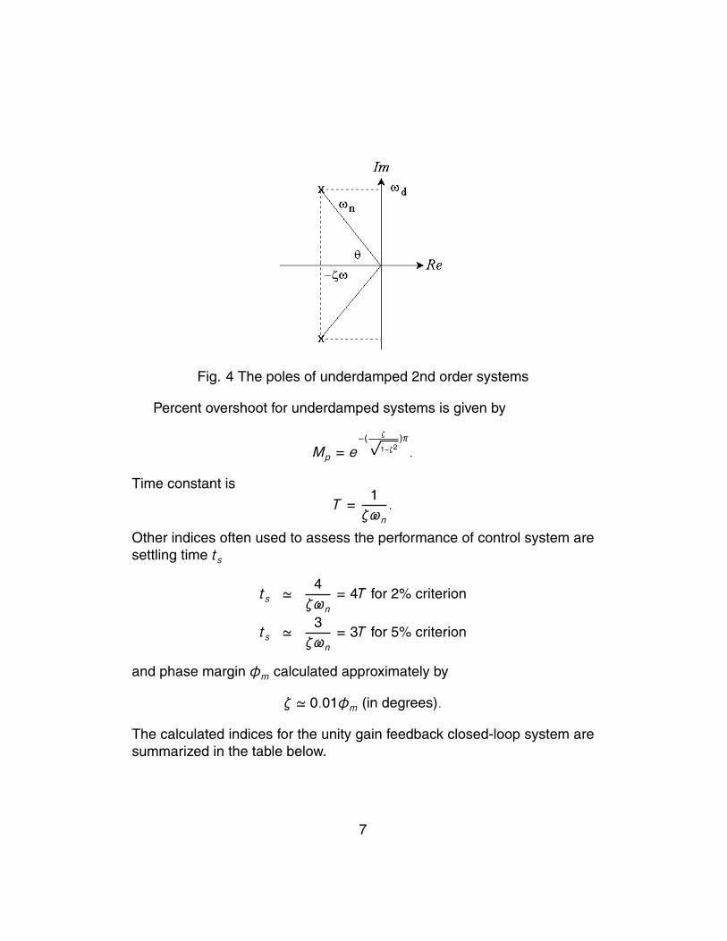
Fig. 4 The poles of underdamped 2nd order systems

Percent overshoot for underdamped systems is given by

Mp = e−( ζ√

1−ζ2)π

.

Time constant is

T =1ζωn

.

Other indices often used to assess the performance of control system aresettling time ts

ts '4ζωn

= 4T for 2% criterion

ts '3ζωn

= 3T for 5% criterion

and phase margin φm calculated approximately by

ζ ' 0.01φm (in degrees).

The calculated indices for the unity gain feedback closed-loop system aresummarized in the table below.

7

ζ 0.03536ωn 0.7071 rad/s 0.1125 Hzωd 0.6614 rad/s 0.1052 HzMp ' 30%T 4 sec.ts (2%) 16 sec.ts (5%) 12 sec.φm 35.36

Comparing these results, it can be concluded that the straight negativefeedback has made the system’s response slower and very underdamped.The time constant of open loop control is 2 seconds. Rough calculation ofthe settling time for the open loop,

e−ts2 = 0.02 (2% criterion)

yields ts = 7.82 seconds. This settling time is also less than that of theclosed loop control.

5 Compensator Design by Root Locus Method

Feedback control can do much better job than what we have seen in oursimple trial of closing the loop with an arbitrary choice of the loop gain.We now consider if it is possible to reduce system’s time constant downto 1 second (twice as fast as the open loop case) and keep the dampingration at about ζ = 0.6. This means that the closed loop poles have to bemoved from where we found for the trial case to the location which satisfiesthe two conditions we chose. The new time constant T = 1/ζωn and thedamping ratio ζ = cosφ = 0.6 determine desired pole locations. They areat s = −1 ± j1.33 compared with s = −0.25 ± j0.66 of the trial case asshown in Fig. 5.

8

Fig. 5 New poles (compensated) and poles of the trial case (uncompensated)

Passive circuits of a first order phase-lead and a phase-lag compen-sator are shown in Fig. 6. The transfer function of either compensatorcircuit will result in the form,

Gp(s) = Kp1 + T s

1 + αTs.

Fig. 6 Passive Circuits of a phase-lead and a phase-lag compensator

For the phase-lead compensator, 0 < α < 1, whereas the phase-lagcompensator takes α > 1. Besides the gain Kp, the difference is its mutualpositions of the pole and the zero. The zero is on the right-hand-side ofthe pole for the phase-lead compensator. In the phase-lag compensator,the pole is on the right-hand-side of the zero. A phase-lead compensator

9

Gp+(s) and a phase-lag compensator Gp−(s) in which the zero and poleare reversed have the transfer functions,

Gp+(s) =s + 0.7s + 1.3

and Gp−(s) =s + 1.3s + 0.7

.

Each case of compensation, phase-lead and phase-lag, is incorporated inthe closed loop system having a transfer forward transfer function,

G(s) =0.5

s(s + 0.5)

to examine general effects on the root loci. The root loci were drawn withthe Matlab commands, rloci(poly([-0.7]),poly([0,-0.5,-1.3])) andrloci(poly([-1.3]),poly([0,-0.5,-0.7])) As seen in Fig. 7, the zeroof the compensator attracts the root locus towards the zero whereas thepole repels the root locus away form the pole.

Fig. 7 Effects of phase-lead and phase-lag compensators on root locus

Referring to Fig. 5, we need to move the root locus from the uncom-pensated pole towards your left to satisfy the new pole locations. Thismeans that we must use a phase-lead compensator. Although the zeromust be at the right-hand-side of the pole, the locations of a pole and azero are arbitrary. Only thing that we have to satisfy is to let the root lo-cus to pass through the new pole location of s = −1 ± j1.33. Usuallythis is accomplished on the basis of try-and-error. For our simple second

10

order system, so called pole-zero cancellation would simplify the tediousprocess of try-and-error. If we set the phase-lead compensator to be

Gp+(s) = Kps + 0.5s + 2

,

The combined open-loop transfer function,

G(s) · Gp+(s) = Kp0.5

s(s + 2)

gives us a straight upright root locus at s = −1 as shown in Fig. 8.

Fig. 8 The root locus plot resulting from pole-zero cancellation

Letting the combined gain of |G(s) · Gp+(s)| to be unity to satisfy thecondition of the root locus, we obtain the compensator gain Kp = 5.55from

|G(s) · Gp+(s)|s=−1±j1.33 = Kp|0.5

s(s + 2)|s=−1±j1.33 = 1.

Thus, our compensator is designed and it is,

Gp+(s) = 5.55s + 0.5s + 2

6 Assessment of the Designed Control System

The designed controller is improved the closed-loop system’s performanceas we have intended.

11

Uncompensated (Sys-I) Compensated (Sys-II)ζ 0.3536 0.6ωd 0.7071 rad/s 1.333 rad/sT 4 sec. 1 sec.

Now, we investigate the power requirement which might have beensubstantially increased because of the shortened time constant from T = 4down to T = 1. The direct input to the robot arm controller, more specif-ically the input to the power supply, should be compared for both of theuncompensated and the compensated control system shown in Fig. 9,respectively.

Fig. 9 Input errors e1 and e2 in the uncompensated and compensated systems

When the input command is to turn the arm exactly one revolution, theinput errors E1(s) and E2(s) are:

E1(s) =1

1 + G(s)1s=

s + 0.5s2 + 0.5s + 0.5

E2(s) =Gp+(s)

1 + G(s)Gp+(s)1s=

5.55(s + 0.5)

s2 + 2s + 2.775.

By using the initial value theorem to find the initial error, which occurs atthe onset of the command, we find:

e1(0) = lims→∞

sE1(s) = 1

12

e2(0) = lims→∞

sE2(s) = 5.55.

Recall that the input to G(s) is expressed in terms of angle θ rather thanthe actual input voltage to the power supply, we would expect the initialvoltage of 5.55×24V to occur when the compensator is incorporated. Thisinput level far exceed the maximum input range of ±28V of the power sup-ply and also the maximum rating of the motor itself.

We can examine position offset using the final value theorem. Positionoffset is the error that remains uncorrected for a step input.

e1(∞) = lims→0

sE1(s) = 0

e2(∞) = lims→0

sE2(s) = 0

Since our system equation is of type I, i.e. G(s) has one pole at s = 0or has one first order integrator 1/s, zero position offset is expected. Asfor velocity offset, we need to use velocity error coefficient Kv to find thevelocity offset ess.

Kv = lims→0

sG(s) = 1, for Sys-I

Kv = lims→0

sGp+(s)G(s) = 1.39, for Sys-II

The velocity offset is the position error when input is a ramp signal 1/s2.Since ess =

1Kv

, ess = 1 for the uncompensated system Sys-I and ess =0.72 for the compensated system Sys-II. Small improvement is gained bythe designed compensator.

7 Compensator Design by Frequency ResponseMethod

The same first order compensator can be designed by using the frequencyresponse method. We still have to use a phase-lead compensator to de-crease the control system’s time constant. The phase-lead compensatornow has a transfer function,

Gc(s) =T1s + 1

T2s + 1.

13

where T1 > T2. DC gain is unity and its high frequency gain is T1/T2. Thefrequency response of this phase-lead compensator is shown in Fig. 10.

Fig. 10 Frequency Response of the Phase-lead Compensator

There are two corner frequencies defined by the amplitude response.The lower corner frequency occurs at ω1 = 1/T1 and the upper cornerfrequency is at ω2 = 1/T2. It can be proved that the maximum leadingphase occurs at ωm =

√ω1ω2. From the frequency response,

Gc(jω) =jω +ω1

jω +ω2

,

the maximum phase obtained at ωm is given by

φm = tan−1 ωmω1− tan−1 ωm

ω2

= tan−1

√

ω2

ω1− tan−1

√

ω1

ω2

Letting α =ω2

ω1, we can express φm as

φm = tan−1 α − 1

2√α

or tanφm =α − 1

2√α.

14

Then, we can prove that

sinφm =α − 1α + 1

.

This is the most important equation that determines the ratio ofω2

ω1for a

desired phase compensation φm. Another important equation to be usedin designing the phase-lead compensator is the gain increase at higherfrequencies, i.e.

Gain = 20 log10

T1

T2

= 20 log10

ω2

ω1= 20 log10 α

The design objective is to design a phase-lead compensator whichgives the overall control system a phase margin of φm = 60. Usually,the loop gain must be determined according to error criteria, separatelyfrom the phase-lead compensator. In our case, we have found the loopgain of 5.55 was inadequate by the previous design based on the root lo-cus. Let us use the loop gain of 1 to alleviate too high input voltage for thepower supply.

The design procedure requires the Bode plot of the open-loop systemwithout a compensator. The following Matlab program allows us to plot thisBode diagram.

% K

% DC Motor: G(s) = --------

% s(Ts+1)

%

clg, clc

K=1;

num=K;

den=[2,1,0];

w=logspace(-2,1,100);

jw=j*w;

H=polyval(num,jw)./polyval(den,jw);

mag=20*log10(abs(H));

phase=angle(H)*180/pi;

subplot(211),semilogx(w,mag,’w’),grid

title(’Magnitude Response’);

xlabel(’frequency in rad/s’),ylabel(’Magnitude in dB’);

subplot(212),semilogx(w,phase,’w’),grid

title(’Phase Response’);

xlabel(’frequency in rad/s’),ylabel(’Phase in degrees’);

15

Fig. 11 Frequency Response of the Phase-lead Compensator

From the obtained Bode plot, we can find that the magnitude cross-overfrequency is 0.45 rad/s and that the phase margin is approximately 45.Therefore, we need to add an additional 15 to meet the required phasemargin of 60. Since a new cross-over frequency needs to be chosen at afrequency higher than the uncompensated system’s cross-over frequency0.45 rad/s, we add 5 to account the further decrease in phase. Therefore,the required phase compensation is φm = 20. Using

sinφm =α − 1α + 1

,

we determine the corner frequency ratio α = ω2/ω1. We obtain α =2.03. Then, we must find the increase in gain introduced by inserting thecompensator.

Gain = 20 log10 α = 6.15 dB

16

Thus, the new cross-over frequency must occur when the magnitude re-sponse of the Bode plot intersects -6.15dB line. The new cross-overfrequency is found to be approximately ωm = 1.0 rad/s. Then, we findtwo corner frequencies ω1 and ω2 from two equations, α = ω2/ω1 andωm =

√ω1ω2. Since ωm = ω1

√α, we find ω1 = 0.70. From ω2 = αω1,

ω2 = 1.42. The designed phase-lead compensator is

Gc(s) =T1s + 1

T2s + 1

=ω2

ω1

s +ω1

s +ω2

= αs +ω1

s +ω2

= 2.03s + 0.70s + 1.42

.

The frequency response of the compensated system by the phase-leadcompensator designed by using the frequency response is calculated bythe following Matlab program.

% 0.5

% DC Motor: G(s) = --------

% s(s+0.5)

% compensated by 2.03(s+0.7)/(s+1.42)

%

clg, clc

K=2.03;

num=K*0.5*poly([-0.7]);

den=poly([0,-0.5,-1.42]);

w=logspace(-2,1,100);

jw=j*w;

H=polyval(num,jw)./polyval(den,jw);

mag=20*log10(abs(H));

phase=angle(H)*180/pi;

subplot(211),semilogx(w,mag,’w’),grid

title(’Magnitude Response’);

xlabel(’frequency in rad/s’),ylabel(’Magnitude in dB’);

subplot(212),semilogx(w,phase,’w’),grid

title(’Phase Response’);

xlabel(’frequency in rad/s’),ylabel(’Phase in degrees’);

17

Fig. 12 Frequency Response of the compensated system

The obtained frequency response is shown in Fig. 12. The phase mar-gin appears to be close to 60.

8 Step Response

The characteristics of the three systems, uncompensated, compensatedwith a controller designed using pole/zero cancellation, and compensatedwith a phase-lead compensator designed by the frequency response method,can be compared from the step response view point. The unit step reponsecan be calculated and displayed by a single Matlab statement step(num,den).The following Matlab program shows how to combine a compensator trans-fer function, a system transfer function, and a feedback transfer func-

18

tion, and generate one combined closed-loop transfer function. This gen-eral Matlab program to construct a closed-loop transfer funtion expects alltransfer functions to be represented by poles and zeros and their gain.Using this program and the built-in function step(num,den)., the unit stepresponses of the above three cases are shown if Fig. 13.

% ----------------------------------------------------

% Finding Closed-Loop Step Response

% From Open-Loop Transfer Function

% K. Takaya Jan, 1998

% ----------------------------------------------------

% G(s)=A1*N1(s)/D1(s), H(s)=A2*N(s)/D2(s)

% Gc(s)=G(s)/1+G(s)H(s)

% =A1*N1(s)D2(s)/D1(s)D2(s)+A1*A2*N1(s)N2(s)

% ----------------------------------------------------

% Specify poles and zeros of G(s) and H(s),

% G(s)=0.5/s(s+0.5), H(s)=1

N1=[]; D1=[0,-0.5];

N2=[]; D2=[];

A1=0.5; A2=1;

% ---------------------(No Compensator)

Num=A1*poly([N1,D2]);

Den1=poly([D1,D2]);

Den2=poly([N1,N2]);

n1=size(Den1,2);

n2=size(Den2,2);

Den=Den1+A1*A2*[zeros(1,n1-n2),Den2];

T=[0:0.1:20];

figure(1); step(Num,Den,T);

% ---------------------(Pole/Zero Cancelled Compensator)

% Specify poles and zeros of G(s), Gc(s) and H(s),

% G(s)=0.5/s(s+0.5), Gc(s)=5.55(s+0.5)/(s+2), H(s)=1

N1=[]; D1=[0,-2.0];

N2=[]; D2=[];

A1=0.5*5.55; A2=1;

% ----------------------------------------------------

Num=A1*poly([N1,D2]);

Den1=poly([D1,D2]);

Den2=poly([N1,N2]);

n1=size(Den1,2);

n2=size(Den2,2);

Den=Den1+A1*A2*[zeros(1,n1-n2),Den2];

T=[0:0.1:20];

figure(2); step(Num,Den,T);

% ---------------------(Phase Margin 60 deg. Compensator)

% Specify poles and zeros of G(s), Gc(s) and H(s),

% G(s)=0.5/s(s+0.5), Gc(s)=2.03(s+0.7)/(s+1.42), H(s)=1

N1=[-0.7]; D1=[0,-0.5,-1.42];

N2=[]; D2=[];

A1=0.5*2.03; A2=1;

% ----------------------------------------------------

Num=A1*poly([N1,D2]);

19

Den1=poly([D1,D2]);

Den2=poly([N1,N2]);

n1=size(Den1,2);

n2=size(Den2,2);

Den=Den1+A1*A2*[zeros(1,n1-n2),Den2];

T=[0:0.1:20];

figure(3); step(Num,Den,T);

Fig. 13 Step Responses of (1) uncompensated system (top), (2) compensatedby pole/zero cancellation (left), and (3) by phase margin 60 (right).

20

9 Assignment No.1

1. Redesign the phase lead compensator without imposing pole-zerocancellation. For a given zero at s = −1, determine only the polee.g. s = −p and an appropriate gain Kp of

Gp+(s) = Kps + 1s + p

such that the time constant T = 1/ζωn = 1.5 sec. and the dampingratio of ζ = cosφ = 0.6 are satisfied for the closed loop system. Usethe root locus method.

2. Redesign the phase lead compensator by the frequency responsemethod to satisfy the phase margin of 70.

The END.

21