1

Polar Codes and Their Quantum-DomainCounterparts

Zunaira Babar, Zeynep B. Kaykac Egilmez, Luping Xiang, Daryus Chandra, Robert G. Maunder, Soon Xin Ng andLajos Hanzo

Abstract—Arikan’s polar codes are capable of approachingShannon’s capacity at a low encoding and decoding complexity,while conveniently supporting rate adaptation. By virtue ofthese attractive features, polar codes have found their way intothe 5G New Radio (NR). Hence, in this paper we provide acomprehensive survey of polar codes, highlighting the majormilestones achieved in the last decade. Furthermore, we alsoprovide tutorial insights into the operation of the polar encoder,decoders as well as their code construction methods. We alsoextend our discussions to quantum polar codes with an emphasison the underlying quantum-to-classical isomorphism and thesyndrome-based quantum polar decoders.

Keywords—channel coding, channel polarization, capacity, polarcodes, quantum error correction.

ACRONYMS

ASIC Application Specific Integrated CircuitAWGN Additive White Gaussian NoiseBCH Bose-Chaudhuri-HocquenghemB-DMC Binary-Input Discrete Memoryless ChannelBEC Binary Erasure ChannelBER Bit Error RateBICM Bit-Interleaved Coded ModulationBICM-ID BICM with Iterative DecodingBLER BLock Error RatioB-MC Binary-input Memoryless ChannelBP Blief PropagationBSC Binary Symmetric ChannelBP Belief PropagationCA-SCL Cyclic Redundancy Check-Aided SCLCA-SCS Cyclic Redundancy Check-Aided SCSCSS Calderbank-Shor-SteaneCNOT Controlled NOTCz Controlled-ZCRC Cyclic Redundancy CheckDE Density EvolutionDMC Discrete Memoryless ChanneleMBB enhanced Mobile BroadBandFEC Forward Error Correction

Z. Babar, Z. B. Kaykac, L. Xiang, D. Chandra, R. G. Maunder, S. X. Ng,and L. Hanzo are with the School of Electronics and Computer Sci-ence, University of Southampton, SO17 1BJ, United Kingdom. Email:{zb2g10,zbk1y15,dc2n14,,rm,sxn,lh}@ecs.soton.ac.uk.

L. Hanzo would like to acknowledge the financial support of the En-gineering and Physical Sciences Research Council projects EP/Noo4558/1,EP/PO34284/1, COALESCE, of the Royal Society’s Global Challenges Re-search Fund Grant as well as of the European Research Council’s AdvancedFellow Grant QuantCom.

FPGA Field Programmable Gate ArrayGA Gaussian ApproximationHARQ Hybrid Automatic Repeat RequestIRCC IRregular Convolutional CodedLDPC Low Density Parity CheckLLR Log-Likelihood RatioLR Likelihood RatioMERA Multi-scale Entanglement Renormalization

AnsatzML Maximum LikelihoodML-SSC Maximum Likelihood Simplified Successive

CancellationmMTC massive Machine Type CommunicationNR New RadioPBCH Physical Broadcast CHannelPC Parity CheckQECC Quantum Error Correction CodeQPSK Quadrature Phase Shift KeyingQSCD Quantum Successive Cancellation DecoderRM Reed-MullerRRNS Redundant Residue Number SystemRS Reed-SolomonSC Successive CancellationSCAN Soft CANcellationSCH Successive Cancellation HybridSCL Successive Cancellation ListSCS Successive Cancellation StackSNR Signal-to-Noise RatioSSC Simplified Successive CancellationSSCL Simplified Successive Cancellation ListTCM Trellis Coded ModulationTTCM Turbo Trellis Coded ModulationURC Unity Rate CodeURLLC Ultra-Reliable Low-Latency CommunicationXOR eXclusive-OR3GPP Third Generation Partnership Project

I. INTRODUCTION

Information is the resolution of uncertainty,Claude Shannon.

The inception of classical coding theory dates back to1948 [1], when Claude Shannon introduced the notion of‘channel capacity’. Explicitly, Shannon predicted in his semi-nal paper [1] that virtually error-free transmission over noisy

2

channels can be achieved by invoking error correction codeshaving a coding rate R lower than the channel capacity Cand having an infinitely long codeword length. The capacityof an Additive White Gaussian Noise (AWGN) channel havingthe bandwidth B (Hz) and the noise power spectral density ofN0/2 (Watts/Hz) per dimension is quantified by the Shannon-Hartley theorem as follows:

C = B log2

(1 +

S

N0B

), (1)

when the average transmitted power is S Watts. Hence,the maximum permissible coding rate of an error correctioncode operating close to capacity is limited by the Signal-to-Noise Ratio (SNR) ( S

N0B) and the bandwidth (B) under the

assumption of tolerating infinite implementation complexityand transmission delay. Similarly, the capacities of a BinarySymmetric Channel (BSC) or a Binary Erasure Channel (BEC)are specified by their respective channel characteristics, i.e. bythe state cross-over probability of the BSC and the erasureprobability of the BEC, again assuming infinite processing andtime resources. However, practical systems can neither affordan infinite implementation complexity nor can they toleratean infinite transmission delay. So, we need optimized codes,which perform close to Shannon’s capacity limit, while guar-anteeing the desired target performance metrics, as illustratedin Fig. 1.

Shannon quantified the capacity limit and proved the ex-istence of ‘capacity-achieving’ codes based on the ‘random-coding’ argument. However, he did not give any recipesfor constructing such capacity-achieving codes. Over the lastseven decades, researchers have endeavored to design optimumcodes, which are capable of operating close to the capacitylimit, while also striking a compelling trade-off amongst thedesired performance metrics of Fig. 1. Broadly speaking, this

Channel Charateristics

System Bandwidth

System Limitations

Bit Error Rate

Coding Rate

Transmission Delay

Effective Throughput

Coding Gain

Implementation Complexity

Performance Metrics

Optimization

Code DesignInput

Input

Output

Fig. 1: Factors driving the code design optimization.

quest has pursued two avenues: the algebraic coding avenueand the probabilistic coding avenue, as portrayed in the stylizedroad map of Fig. 2. Algebraic coding was the main research av-enue for the first few decades. The aim of this coding paradigmis to design powerful codes by exploiting finite-field arithmeticto maximize the minimum Hamming distance1 between thecodewords for a given coding rate, or more specifically forthe given information word length k and codeword length n.This has given rise to a range of popular coding families,which includes for example Hamming codes [2], Reed-Muller(RM) codes [3], [4], Bose-Chaudhuri-Hocquenghem (BCH)codes [5], [6], Reed-Solomon (RS) codes [7] and RedundantResidue Number System (RRNS) codes [8], [9]. Unfortunately,maximizing the minimum distance of codewords along thealgebraic avenue of Fig. 2 does not promise a ‘capacity-achieving’ design. Nonetheless, algebraic codes have foundtheir way into practical applications by virtue of their strongerror correction capabilities (or equivalently low Bit Error Rate(BER) floors). Explicitly, these codes are useful, when the

1The Hamming distance between two vectors is equal to the number ofpositions at which the corresponding elements (bits or symbols) differ.

Shannon’s

Capacity

Maximum

Distance

MinimumCorrection

Ham

ming R

oad

BC

H R

oad

RS

Road

RR

NS R

oad

Algebraic Avenue

TT

CM

Lane

Turbo RoadConvolutional R

oad

TCM Road

BICM Road

UR

C L

ane

IRC

C L

ane

BIC

M−ID

Lane

Pol

ar R

oad

LD

PC

Road

Probabilistic AvenueError

RM

Road

Fig. 2: Road map portraying the evolution of classical channel coding theory. The algebraic avenue aims at maximizing theminimum distance, while the probabilistic avenue leads to capacity approaching designs.

3

received information is in the form of hard decisions. Forexample, RS codes are used in magnetic tape and disk storageas well as in several standardized systems, such as the deep-space coding standard [10], where they typically constitute anouter layer2 of error correction (known as the outer code) toreduce the BER floor resulting from the failure of the innerlayer of error correction (called the inner code).

In contrast to the algebraic coding avenue, the probabilisticcoding avenue has succeeded in paving the way to capacity.Explicitly, the probabilistic coding avenue of Fig. 2 is in-spired by Shannon’s random coding philosophy and strivesfor achieving a reasonable trade-off between the performanceand the complexity. This design avenue has led to the con-struction of convolutional codes [11], Low Density ParityCheck (LDPC) codes [12]–[14], turbo codes [15], [16] aswell as polar codes [17]. The probabilistic coding paradigmalso includes various ‘turbo-like’ iterative coding schemes, forexample turbo BCH codes [18], turbo Hamming codes [19],and the Unity Rate Code (URC)-assisted and IRregular Con-volutional Coded (IRCC) concatenated schemes of [20], [21],as well as the coded modulation schemes, including TrellisCoded Modulation (TCM) [22]–[24], Bit-Interleaved CodedModulation (BICM) [25], [26], BICM with Iterative Decod-ing (BICM-ID) [27], and Turbo Trellis Coded Modulation(TTCM) [28]. In particular, the turbo and LDPC codes madeit possible to operate arbitrarily close to the Shannon limit,while the polar codes finally managed to provably approachthe capacity, albeit at infinitely long codeword lengths. Despitebeing a relatively immature coding scheme, polar coding hasproved to be a fierce competitor of turbo and LDPC codes, bothof which have been ruling for over two decades. Polar codeshave already found their way into the 5G New Radio (NR)for the control channels of the enhanced Mobile BroadBand(eMBB) and the Ultra-Reliable Low-Latency Communication(URLLC) use-cases as well as for the Physical BroadcastCHannel (PBCH). Polar codes have also been identified aspotential candidates for the data and control channels of themassive Machine Type Communication (mMTC) use-cases.

Polar codes emerged in at once, when the apprehensionthat ‘coding is dead’ started looming again3. Hence, thediscovery of polar codes re-energized the coding communityand equipped them with a radically different approach forapproaching Shannon’s capacity. In addition to its influenceon the classical coding theory, polar codes have also attractedconsiderable attention within the quantum research community.Motivated by the growing interest in polar codes, in this paperwe provide a comprehensive survey of both the classical as wellas quantum polar codes, taking the readers through the majormilestones achieved and providing a slow-paced tutorial onthe related encoding and decoding algorithms. This tutorial

2Outer layer is with respect to the channel. The inner layer is closer to thechannel.

3The notion that ‘coding is dead’ first officially surfaced in the IEEECommunication Theory Workshop held in St. Petersburg, Florida, in April1971, where a group of coding theorists concluded that there was nothingmore to do in coding theory. This workshop became famous as the ‘coding isdead’ workshop.

paper sets the necessary background for understanding theoperation of the Third Generation Partnership Project (3GPP)5G NR polar codes, which have been surveyed in [29], [30].It is pertinent to mention here that, to the best of authors’knowledge, only two survey papers [31], [32] exist on polarcodes at the time of writing. In [31], the author’s haveprovided a succinct overview of the fundamental conceptspertaining to polar codes, including the encoding, decoding andconstruction methods, while [32] focuses on the ApplicationSpecific Integrated Circuit (ASIC) implementation of polardecoders. By contrast, this paper has a broader scope, sincewe provide in-depth tutorial insights (with explicit examples)as well as a comprehensive survey on polar encoders, decodersas well as polar code construction methods.

Fig. 3 provides the overview of the paper. We commenceour discourse in Section II, where we discuss Arikan’s channelpolarization philosophy, which is the key to approaching Shan-non’s capacity. We then survey the polar encoding and decod-ing algorithms in Section III and Section IV, respectively, withdetailed tutorial insights. Continuing further our discussions,we present the polar code design principles and guidelines inSection V. In Section VI, we detail the transition from theclassical to the quantum channel polarization by identifyingthe underlying isomorphism. Based on the isomorphism ofSection VI, we proceed to quantum polar codes in Section VII.Finally, we conclude our discussions in Section VIII.

II. THE PHILOSOPHY OF CHANNEL POLARIZATION

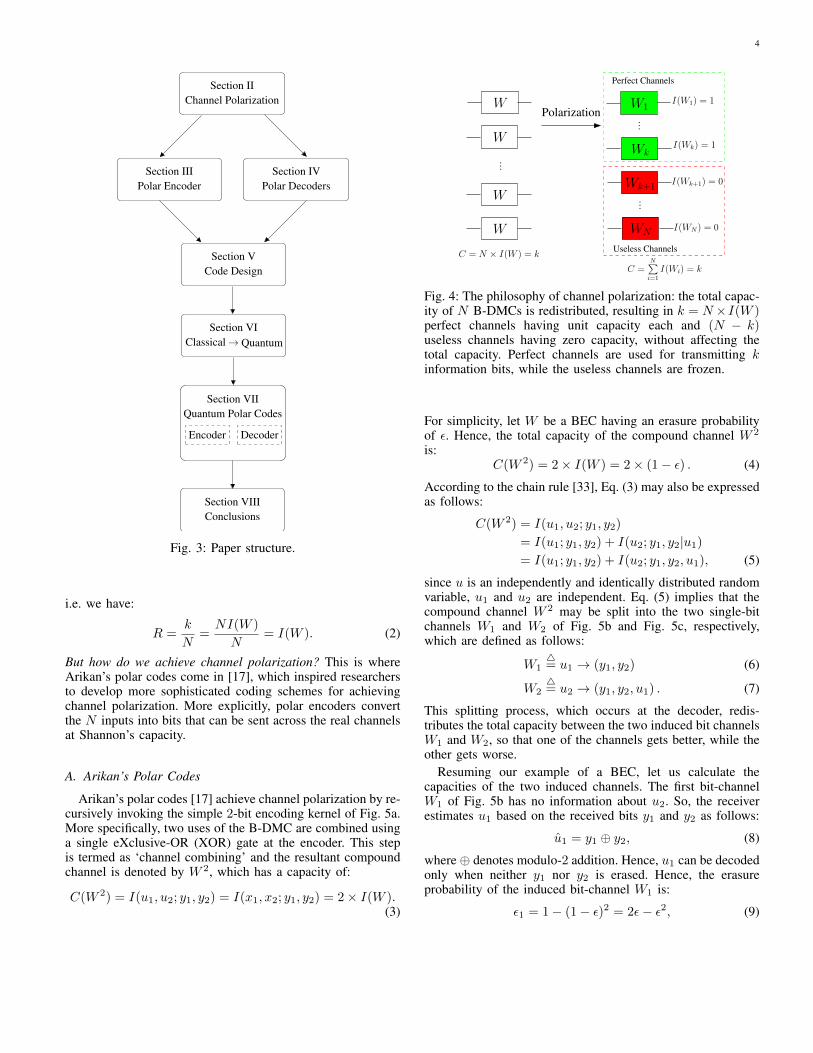
Polar codes rely on the phenomenon of channel polarization,which is the key contributor towards approaching Shannon’scapacity. Channel polarization is basically the process ofredistributing channel capacities among the various instances,or more precisely uses, of a transmission channel withoutaffecting, while conserving the total capacity, as encapsulatedin Fig. 4. Explicitly, channel polarization implies that a setof given channels is polarized into perfect and useless (orcompletely random) channels, having capacities of 1 and 0,respectively. This in turn makes the channel coding problemtrivial, since the perfect channels may be used for transmittinguncoded information without any errors, while the uselesschannels can be discarded.

Let us consider N uses of a B-DMC W , each having acapacity of I(W ), as exemplified in Fig. 4. In the asymptoticregion, i.e. when N is infinitely large, channel polarizationresults in k = N × I(W ) perfect channels having near-1capacity and (N −k) useless channels having near-0 capacity.Thereafter, k information bits are sent uncoded (rate-1) throughthe induced perfect channels, while the (N − k) inputs tothe induced useless channels are frozen, implying that knownredundant bits are sent across these channels (rate-0)4. Hence,the resultant coding rate is equivalent to the channel capacity,

4An induced bit-channel is a hypothetical end-to-end channel, which con-sists of the encoder, the real channel and the decoder, as discussed further inSection II-A. Hence, the information sent across the real channels is encoded.However, the resulting induced bit-channels may be viewed as rate-1 andrate-0 channels, since they exhibit a capacity of 0 and 1, respectively.

4

Channel Polarization

Section II

Polar Decoders

Section IV

Polar Encoder

Section III

Section VI

QuantumClassical

Encoder

Conclusions

Section VIII

Decoder

Section VII

Quantum Polar Codes

Section V

Code Design

→

Fig. 3: Paper structure.

i.e. we have:

R =k

N=NI(W )

N= I(W ). (2)

But how do we achieve channel polarization? This is whereArikan’s polar codes come in [17], which inspired researchersto develop more sophisticated coding schemes for achievingchannel polarization. More explicitly, polar encoders convertthe N inputs into bits that can be sent across the real channelsat Shannon’s capacity.

A. Arikan’s Polar Codes

Arikan’s polar codes [17] achieve channel polarization by re-cursively invoking the simple 2-bit encoding kernel of Fig. 5a.More specifically, two uses of the B-DMC are combined usinga single eXclusive-OR (XOR) gate at the encoder. This stepis termed as ‘channel combining’ and the resultant compoundchannel is denoted by W 2, which has a capacity of:

C(W 2) = I(u1, u2; y1, y2) = I(x1, x2; y1, y2) = 2× I(W ).(3)

Polarization

Perfect Channels

Useless Channels

W

W

W

W ...

...

Wk

Wk+1

WN

...

W1

C = N × I(W ) = k

I(W1) = 1

I(Wk) = 1

I(Wk+1) = 0

I(WN) = 0

C =N∑i=1

I(Wi) = k

Fig. 4: The philosophy of channel polarization: the total capac-ity of N B-DMCs is redistributed, resulting in k = N ×I(W )perfect channels having unit capacity each and (N − k)useless channels having zero capacity, without affecting thetotal capacity. Perfect channels are used for transmitting kinformation bits, while the useless channels are frozen.

For simplicity, let W be a BEC having an erasure probabilityof ε. Hence, the total capacity of the compound channel W 2

is:C(W 2) = 2× I(W ) = 2× (1− ε) . (4)

According to the chain rule [33], Eq. (3) may also be expressedas follows:

C(W 2) = I(u1, u2; y1, y2)

= I(u1; y1, y2) + I(u2; y1, y2|u1)= I(u1; y1, y2) + I(u2; y1, y2, u1), (5)

since u is an independently and identically distributed randomvariable, u1 and u2 are independent. Eq. (5) implies that thecompound channel W 2 may be split into the two single-bitchannels W1 and W2 of Fig. 5b and Fig. 5c, respectively,which are defined as follows:

W14= u1 → (y1, y2) (6)

W24= u2 → (y1, y2, u1) . (7)

This splitting process, which occurs at the decoder, redis-tributes the total capacity between the two induced bit channelsW1 and W2, so that one of the channels gets better, while theother gets worse.

Resuming our example of a BEC, let us calculate thecapacities of the two induced channels. The first bit-channelW1 of Fig. 5b has no information about u2. So, the receiverestimates u1 based on the received bits y1 and y2 as follows:

u1 = y1 ⊕ y2, (8)

where ⊕ denotes modulo-2 addition. Hence, u1 can be decodedonly when neither y1 nor y2 is erased. Hence, the erasureprobability of the induced bit-channel W1 is:

ε1 = 1− (1− ε)2 = 2ε− ε2, (9)

5

Wu2 x2

Wu1 x1

W 2

y2

y1

G2

(a) Channel combining.

Wu2 x2

Wx1

y2

y1

W1 : u1 → (y1, y2)

u1

(b) Channel splitting: first bit channel.

Wx2

Wx1

y2

y1

W2 : u2 → (y1, y2, u1)

u2

u1

u1

(c) Channel splitting: second bit channel.

Fig. 5: Arikan’s 2-bit polar code, relying on channel combiningand channel splitting for channel polarization.

which is worse than that of the original channel W . Conse-quently, W1 is the worse channel, also denoted as W−, havinga reduced capacity of:

I(W−) = 1− ε1 = 1− 2ε+ ε2. (10)

The second bit channel of Fig. 5c outputs u1 as well as y1and y2. Explicitly, the availability of u1 implies that we havea ’genie’ decoder or a side-information channel, which revealsthe value of u1. Consequently, u2 can be decoded as long asneither y1 nor y2 is erased. Hence, the erasure probability ofthe induced channel W2 is:

ε2 = ε2, (11)

which is lower than that of the original channel W . Thisimplies that W2 is the better channel, also denoted as W+,

which has a capacity of:

I(W+) = 1− ε2 = 1− ε2. (12)

Based on Eq. (10) and Eq. (12), we may conclude that:

I(W−) ≤ I(W ) ≤ I(W+), (13)

which implies that W− (or equivalently W1) tends to polarizetowards zero-capacity, while W+ (or equivalently W2) tendsto polarize towards unit capacity. It is pertinent to mention herethat the equality in Eq. (13) holds only when W is an extremechannel having a capacity of either 0 or 1. Furthermore, thetotal capacity remains unaffected, since we have:

I(W−) + I(W−) = 2× I(W ). (14)

To elaborate further, let us assume that ε = 0.5, hence wehave:

I(W ) = 0.5

I(W1) = I(W−) = 0.25

I(W2) = I(W+) = 0.75, (15)

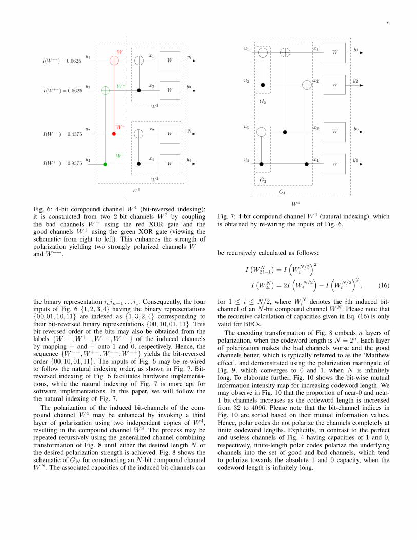
where we may observe that the value of I(W−) gets closer tozero, while that of I(W+) gets closer to one. The impact ofchannel polarization may be enhanced by recursively invokingthe basic encoding kernel of Fig. 5a, which is labeled ‘G2’.More specifically, as exemplified in Fig. 6, a compoundchannel W 4 can be constructed by using two copies of thecompound channel W 2. In the first layer of polarization,two independent copies of W 2 are invoked, inducing twogood channels W+ and two bad channels W−, which havethe capacities of 0.25 and 0.75, respectively, for ε = 0.5.In the second layer of polarization, the bad channels arecoupled using the encoding kernel G2 of Fig. 5a, which issimply a XOR gate marked in red in Fig. 6. Recall that theencoding transformation of Fig. 5a yields a bad and a goodchannel, whose capacities may be calculated using Eq. (10)and Eq. (12), respectively. Consequently, the red XOR gate ofFig. 6 polarizes the two W− channels into a worse channelW−− and a better channel W−+, having capacities of 0.0625and 0.4375, respectively. We may observe here that the secondlayer of polarization polarizes the first channel more towardsthe zero capacity, while the capacity of the other channel tendsto increase towards one.

Similarly, the second layer of polarization couples the twogood channels W+ using the XOR gate marked in green inFig. 6. This second XOR gate induces the channels W+−

and W++ having capacities of 0.5625 and 0.9375, respec-tively. Hence, a two-layered polarization yields two stronglypolarized channels W−− and W++, which exhibit a higherdegree of polarization than the channels W− and W+. Itis important to point out that the bits in Fig. 6 are indexedaccording to their decoding order, which will be discussedfurther in Section IV. Furthermore, it may also be observedthat the bits in Fig. 6 follow a bit-reversed indexing. Ex-plicitly, bit reversing implies that a number i ∈ {1, N}having the n-bit binary representation i1i2 . . . in, for n =log2N , is mapped onto its bit-reversed counterpart having

6

Wx4

Wx2

W 2

y4

y2

Wx3

Wx1

W 2

y3

y1

W 4

W−

W+

u1

u3

u2

u4

W−

W+

I(W−−) = 0.0625

I(W+−) = 0.5625

I(W−+) = 0.4375

I(W++) = 0.9375

Fig. 6: 4-bit compound channel W 4 (bit-reversed indexing):it is constructed from two 2-bit channels W 2 by couplingthe bad channels W− using the red XOR gate and thegood channels W+ using the green XOR gate (viewing theschematic from right to left). This enhances the strength ofpolarization yielding two strongly polarized channels W−−and W++.

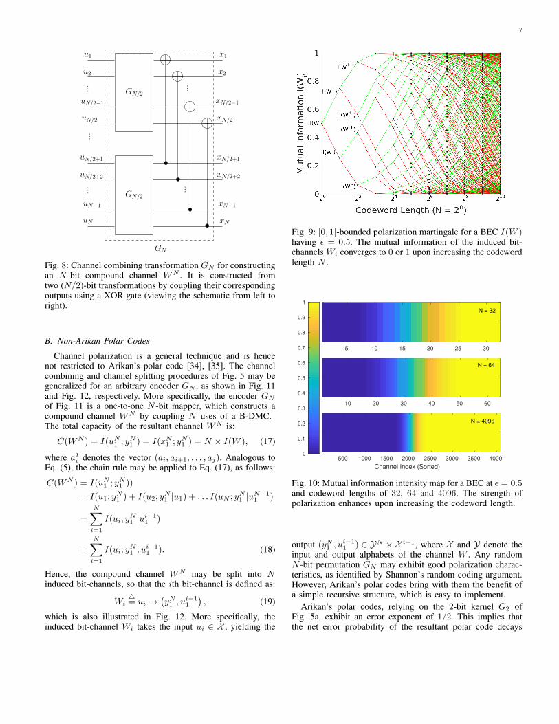
the binary representation inin−1 . . . i1. Consequently, the fourinputs of Fig. 6 {1, 2, 3, 4} having the binary representations{00, 01, 10, 11} are indexed as {1, 3, 2, 4} corresponding totheir bit-reversed binary representations {00, 10, 01, 11}. Thisbit-reversed order of the bits may also be obtained from thelabels {W−−,W+−,W−+,W++} of the induced channelsby mapping + and − onto 1 and 0, respectively. Hence, thesequence {W−−,W+−,W−+,W++} yields the bit-reversedorder {00, 10, 01, 11}. The inputs of Fig. 6 may be re-wiredto follow the natural indexing order, as shown in Fig. 7. Bit-reversed indexing of Fig. 6 facilitates hardware implementa-tions, while the natural indexing of Fig. 7 is more apt forsoftware implementations. In this paper, we will follow thethe natural indexing of Fig. 7.

The polarization of the induced bit-channels of the com-pound channel W 4 may be enhanced by invoking a thirdlayer of polarization using two independent copies of W 4,resulting in the compound channel W 8. The process may berepeated recursively using the generalized channel combiningtransformation of Fig. 8 until either the desired length N orthe desired polarization strength is achieved. Fig. 8 shows theschematic of GN for constructing an N -bit compound channelWN . The associated capacities of the induced bit-channels can

x4

x3

x2

x1

W

W

y4

y3

W

W

y2

y1u1

u2

u3

u4

G2

G2

G4

W 4

Fig. 7: 4-bit compound channel W 4 (natural indexing), whichis obtained by re-wiring the inputs of Fig. 6.

be recursively calculated as follows:

I(WN

2i−1)= I

(W

N/2i

)2

I(WN

2i

)= 2I

(W

N/2i

)− I

(W

N/2i

)2, (16)

for 1 ≤ i ≤ N/2, where WNi denotes the ith induced bit-

channel of an N -bit compound channel WN . Please note thatthe recursive calculation of capacities given in Eq. (16) is onlyvalid for BECs.

The encoding transformation of Fig. 8 embeds n layers ofpolarization, when the codeword length is N = 2n. Each layerof polarization makes the bad channels worse and the goodchannels better, which is typically referred to as the ‘Mattheweffect’, and demonstrated using the polarization martingale ofFig. 9, which converges to 0 and 1, when N is infinitelylong. To elaborate further, Fig. 10 shows the bit-wise mutualinformation intensity map for increasing codeword length. Wemay observe in Fig. 10 that the proportion of near-0 and near-1 bit-channels increases as the codeword length is increasedfrom 32 to 4096. Please note that the bit-channel indices inFig. 10 are sorted based on their mutual information values.Hence, polar codes do not polarize the channels completely atfinite codeword lengths. Explicitly, in contrast to the perfectand useless channels of Fig. 4 having capacities of 1 and 0,respectively, finite-length polar codes polarize the underlyingchannels into the set of good and bad channels, which tendto polarize towards the absolute 1 and 0 capacity, when thecodeword length is infinitely long.

7

uN

uN−1

uN/2+1

uN/2+2

u1

u2

...

uN/2

uN/2−1

...

...

xN

xN−1

xN/2+1

xN/2+2

x1

x2

xN/2−1

xN/2

GN/2

...

...GN/2

GN

Fig. 8: Channel combining transformation GN for constructingan N -bit compound channel WN . It is constructed fromtwo (N/2)-bit transformations by coupling their correspondingoutputs using a XOR gate (viewing the schematic from left toright).

B. Non-Arikan Polar Codes

Channel polarization is a general technique and is hencenot restricted to Arikan’s polar code [34], [35]. The channelcombining and channel splitting procedures of Fig. 5 may begeneralized for an arbitrary encoder GN , as shown in Fig. 11and Fig. 12, respectively. More specifically, the encoder GNof Fig. 11 is a one-to-one N -bit mapper, which constructs acompound channel WN by coupling N uses of a B-DMC.The total capacity of the resultant channel WN is:

C(WN ) = I(uN1 ; yN1 ) = I(xN1 ; yN1 ) = N × I(W ), (17)

where aji denotes the vector (ai, ai+1, . . . , aj). Analogous toEq. (5), the chain rule may be applied to Eq. (17), as follows:

C(WN ) = I(uN1 ; yN1 ))

= I(u1; yN1 ) + I(u2; y

N1 |u1) + . . . I(uN ; yN1 |uN−11 )

=

N∑

i=1

I(ui; yN1 |ui−11 )

=

N∑

i=1

I(ui; yN1 , u

i−11 ). (18)

Hence, the compound channel WN may be split into Ninduced bit-channels, so that the ith bit-channel is defined as:

Wi4= ui →

(yN1 , u

i−11

), (19)

which is also illustrated in Fig. 12. More specifically, theinduced bit-channel Wi takes the input ui ∈ X , yielding the

Fig. 9: [0, 1]-bounded polarization martingale for a BEC I(W )having ε = 0.5. The mutual information of the induced bit-channels Wi converges to 0 or 1 upon increasing the codewordlength N .

5 10 15 20 25 30

10 20 30 40 50 60

500 1000 1500 2000 2500 3000 3500 4000

Channel Index (Sorted)

0

0.1

0.2

0.3

0.4

0.5

0.6

0.7

0.8

0.9

1

N = 64

N = 4096

N = 32

Fig. 10: Mutual information intensity map for a BEC at ε = 0.5and codeword lengths of 32, 64 and 4096. The strength ofpolarization enhances upon increasing the codeword length.

output (yN1 , ui−11 ) ∈ YN × X i−1, where X and Y denote the

input and output alphabets of the channel W . Any randomN -bit permutation GN may exhibit good polarization charac-teristics, as identified by Shannon’s random coding argument.However, Arikan’s polar codes bring with them the benefit ofa simple recursive structure, which is easy to implement.

Arikan’s polar codes, relying on the 2-bit kernel G2 ofFig. 5a, exhibit an error exponent of 1/2. This implies thatthe net error probability of the resultant polar code decays

8

WxN yN

W

W

y2

y1

x2

x1

GN

uN

u1

u2

... ...

WN

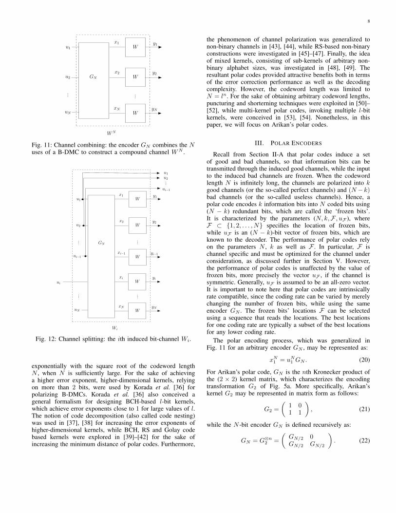
Fig. 11: Channel combining: the encoder GN combines the Nuses of a B-DMC to construct a compound channel WN .

Wxi−1 yi−1ui−1

WxN yNuN

W

W

y2

y1

x2

x1u1

u2

......

... ...

Wi

GN

ui−1

u2...

u1

Wxi yi

ui

Fig. 12: Channel splitting: the ith induced bit-channel Wi.

exponentially with the square root of the codeword lengthN , when N is sufficiently large. For the sake of achievinga higher error exponent, higher-dimensional kernels, relyingon more than 2 bits, were used by Korada et al. [36] forpolarizing B-DMCs. Korada et al. [36] also conceived ageneral formalism for designing BCH-based l-bit kernels,which achieve error exponents close to 1 for large values of l.The notion of code decomposition (also called code nesting)was used in [37], [38] for increasing the error exponents ofhigher-dimensional kernels, while BCH, RS and Golay codebased kernels were explored in [39]–[42] for the sake ofincreasing the minimum distance of polar codes. Furthermore,

the phenomenon of channel polarization was generalized tonon-binary channels in [43], [44], while RS-based non-binaryconstructions were investigated in [45]–[47]. Finally, the ideaof mixed kernels, consisting of sub-kernels of arbitrary non-binary alphabet sizes, was investigated in [48], [49]. Theresultant polar codes provided attractive benefits both in termsof the error correction performance as well as the decodingcomplexity. However, the codeword length was limited toN = ln. For the sake of obtaining arbitrary codeword lengths,puncturing and shorterning techniques were exploited in [50]–[52], while multi-kernel polar codes, invoking multiple l-bitkernels, were conceived in [53], [54]. Nonetheless, in thispaper, we will focus on Arikan’s polar codes.

III. POLAR ENCODERS

Recall from Section II-A that polar codes induce a setof good and bad channels, so that information bits can betransmitted through the induced good channels, while the inputto the induced bad channels are frozen. When the codewordlength N is infinitely long, the channels are polarized into kgood channels (or the so-called perfect channels) and (N −k)bad channels (or the so-called useless channels). Hence, apolar code encodes k information bits into N coded bits using(N − k) redundant bits, which are called the ‘frozen bits’.It is characterized by the parameters (N, k,F , uF ), whereF ⊂ {1, 2, . . . , N} specifies the location of frozen bits,while uF is an (N − k)-bit vector of frozen bits, which areknown to the decoder. The performance of polar codes relyon the parameters N , k as well as F . In particular, F ischannel specific and must be optimized for the channel underconsideration, as discussed further in Section V. However,the performance of polar codes is unaffected by the value offrozen bits, more precisely the vector uF , if the channel issymmetric. Generally, uF is assumed to be an all-zero vector.It is important to note here that polar codes are intrinsicallyrate compatible, since the coding rate can be varied by merelychanging the number of frozen bits, while using the sameencoder GN . The frozen bits’ locations F can be selectedusing a sequence that reads the locations. The best locationsfor one coding rate are typically a subset of the best locationsfor any lower coding rate.

The polar encoding process, which was generalized inFig. 11 for an arbitrary encoder GN , may be represented as:

xN1 = uN1 GN . (20)

For Arikan’s polar code, GN is the nth Kronecker product ofthe (2 × 2) kernel matrix, which characterizes the encodingtransformation G2 of Fig. 5a. More specifically, Arikan’skernel G2 may be represented in matrix form as follows:

G2 =

(1 01 1

), (21)

while the N -bit encoder GN is defined recursively as:

GN = G⊗n2 =

(GN/2 0GN/2 GN/2

). (22)

9

Hence, Arikan’s polar code has a recursive structure invokingn = log2N layers of polarization and each layer of po-larization uses N/2 XOR gates, as previously illustrated inFig. 8. Hence, the encoding operation of Eq. (22) imposesa complexity of O(N log2N). We may also notice fromEq. (22) that polar codes assume a non-systematic structure.Later, systematic polar codes were derived in [55]–[58], whichoutperformed the classic non-systematic polar codes in termsof the BER, while retaining the same BLock Error Ratio(BLER) and encoding, decoding complexity. We restrict ourdiscussions to the classic non-systematic polar codes in thispaper.

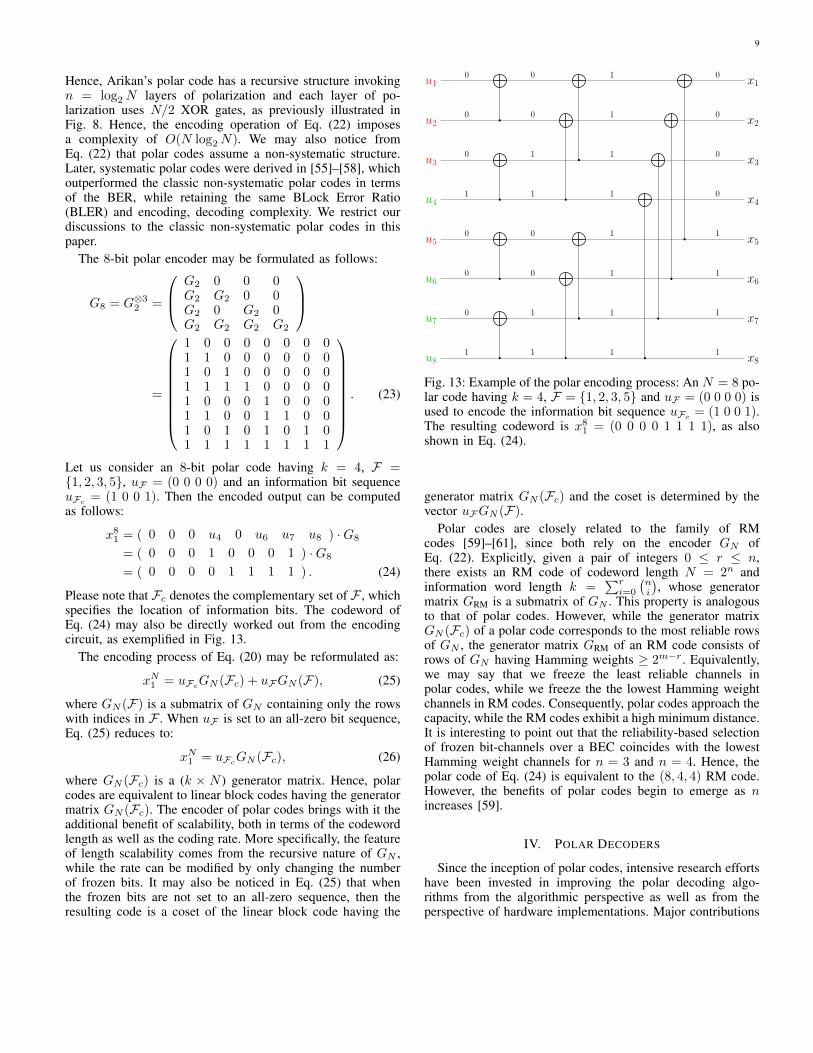
The 8-bit polar encoder may be formulated as follows:

G8 = G⊗32 =

G2 0 0 0G2 G2 0 0G2 0 G2 0G2 G2 G2 G2

=

1 0 0 0 0 0 0 01 1 0 0 0 0 0 01 0 1 0 0 0 0 01 1 1 1 0 0 0 01 0 0 0 1 0 0 01 1 0 0 1 1 0 01 0 1 0 1 0 1 01 1 1 1 1 1 1 1

. (23)

Let us consider an 8-bit polar code having k = 4, F ={1, 2, 3, 5}, uF = (0 0 0 0) and an information bit sequenceuFc = (1 0 0 1). Then the encoded output can be computedas follows:

x81 = ( 0 0 0 u4 0 u6 u7 u8 ) ·G8

= ( 0 0 0 1 0 0 0 1 ) ·G8

= ( 0 0 0 0 1 1 1 1 ) . (24)

Please note that Fc denotes the complementary set of F , whichspecifies the location of information bits. The codeword ofEq. (24) may also be directly worked out from the encodingcircuit, as exemplified in Fig. 13.

The encoding process of Eq. (20) may be reformulated as:

xN1 = uFcGN (Fc) + uFGN (F), (25)

where GN (F) is a submatrix of GN containing only the rowswith indices in F . When uF is set to an all-zero bit sequence,Eq. (25) reduces to:

xN1 = uFcGN (Fc), (26)

where GN (Fc) is a (k × N ) generator matrix. Hence, polarcodes are equivalent to linear block codes having the generatormatrix GN (Fc). The encoder of polar codes brings with it theadditional benefit of scalability, both in terms of the codewordlength as well as the coding rate. More specifically, the featureof length scalability comes from the recursive nature of GN ,while the rate can be modified by only changing the numberof frozen bits. It may also be noticed in Eq. (25) that whenthe frozen bits are not set to an all-zero sequence, then theresulting code is a coset of the linear block code having the

u3

u5

u4

u6

u7

u8

x1

x2

x3

x4

x5

x6

x7

x8

0

0

0

1

0

0

0

1

0

0

1

1

0

0

1

1

1

1

1

1

1

1

1

1

0

0

0

0

1

1

1

1

u2

u1

Fig. 13: Example of the polar encoding process: An N = 8 po-lar code having k = 4, F = {1, 2, 3, 5} and uF = (0 0 0 0) isused to encode the information bit sequence uFc = (1 0 0 1).The resulting codeword is x81 = (0 0 0 0 1 1 1 1), as alsoshown in Eq. (24).

generator matrix GN (Fc) and the coset is determined by thevector uFGN (F).

Polar codes are closely related to the family of RMcodes [59]–[61], since both rely on the encoder GN ofEq. (22). Explicitly, given a pair of integers 0 ≤ r ≤ n,there exists an RM code of codeword length N = 2n andinformation word length k =

∑ri=0

(ni

), whose generator

matrix GRM is a submatrix of GN . This property is analogousto that of polar codes. However, while the generator matrixGN (Fc) of a polar code corresponds to the most reliable rowsof GN , the generator matrix GRM of an RM code consists ofrows of GN having Hamming weights ≥ 2m−r. Equivalently,we may say that we freeze the least reliable channels inpolar codes, while we freeze the the lowest Hamming weightchannels in RM codes. Consequently, polar codes approach thecapacity, while the RM codes exhibit a high minimum distance.It is interesting to point out that the reliability-based selectionof frozen bit-channels over a BEC coincides with the lowestHamming weight channels for n = 3 and n = 4. Hence, thepolar code of Eq. (24) is equivalent to the (8, 4, 4) RM code.However, the benefits of polar codes begin to emerge as nincreases [59].

IV. POLAR DECODERS

Since the inception of polar codes, intensive research effortshave been invested in improving the polar decoding algo-rithms from the algorithmic perspective as well as from theperspective of hardware implementations. Major contributions

10

Algorithmic Developments Hardware Implementations

Belief Propagation (BP) and Successive Cancellation (SC) decoder [17], [62] 2009−BP decoding improved by exploiting overcomplete factor graphs [63] −

Trellis-based Maximum Likelihood (ML) decoder for short polar codes [64] −Linear programming based polar decoder for BEC [65] 2010−

−Log Likelihood Ratio (LLR)-based SC decoder [66], [67] 2011− Hardware implementations relying on improved scheduling for (LLR)-based SC

decoder [66], [67]Simplified Successive Cancellation (SSC) decoder [68] −Successive Cancellation List (SCL) decoder [69]–[71] −

Successive Cancellation Stack (SCS) decoder [72] 2012− Pre-computed look-ahead scheduling for reducing the latency of SC decoder [73]Cyclic Redundancy Check (CRC)-aided SCL (CA-SCL) and SCS (CA-SCS)

decoders [70], [74] −Adaptive CA-SCL decoder [75] −

Multistage polar decoder [76] −ML sphere decoder for short polar codes [77] −

Successive Cancellation Hybrid (SCH) decoder [78] 2013− Semi-parallel architecture for SC decoder [79]Maximum Likelihood Simplified Successive Cancellation (ML-SSC) decoder [80] − Scalable semi-parallel implementation of SC decoder [81], [82]

Soft CANcellation (SCAN) decoder [83], [84] − Field Programmable Gate Array (FPGA) implementation of BP decoder [85]− Two-phase SC decoder architecture having a lower complexity and memory

utilization, and a higher throughput [86]− Overlapped SC decoder architecture [87]

ML-SSC improved [88] 2014− Flexible and high throughput architecture of improved ML-SSC decoder [88]Modified BP [89], [90] − Hardware implementation of SCL decoder [91]

Early terminated BP decoder [92]: − Efficient partial-sum network architecture for semi-parallel SC decoder [93]Low-latency CA-SCL decoder [94] − Architecture of SSC decoder [95]

Symbol-based SC and SCL decoders [96], [97] − Architecture of 2-bit SC decoder [98]SC flip decoder [99] −

Error exponent of SCL investigated [100] 2015−LLR-based SCL decoder [101] − Hardware architecture of LLR-based SCL decoder [101]

− Architecture of a low-latency multi-bit SCL decoder [102]− Metric sorter architecture for SCL decoder [103]− Low-latency SCL decoder relying on double thresholding based list pruning [104],

[105]Reduced-complexity early terminated BP decoder [106] 2016− Hardware Architecture of low-latency CA-SCL decoder [107] relying on [94]

The reduced latency ideas of [88] extended to the SCL decoder [108] − Implementation of adaptive throughput-area efficient SCL decoder invoking ap-proximate ML decoding components [109]

Tree pruning for low-latency SCL decoding [110] − Sphere decoding based architecture of SCL decoder [111]Reduced-complexity SCL decoder [112] − Improved metric sorter architecture for SCL decoder [113]

Simplified Successive Cancellation List (SSCL) decoder avoiding redundantcalculations [114] − Hardware implementation of CA-SCL based on distributed sorting [115]

Parity-check-aided polar decoding [116] −Reduced latency SSCL decoder [117] 2017− Hardware implementation of SSCL decoder [117]

Unsorted SCL decoder [118] − Hardware implementation of low-latency BP decoder [119]Syndrome-based SC decoder [120] − Two-step metric sorter architecture for parallel SCL decoder [121]

Soft SCL decoder for systematic codes [122], [123] − Memory efficient architectures for SC and SCL decoders [124]Reduced-latency SSC flip decoder [125] 2018−

BP list decoder [126] − Hardware architecture of multi-bit double thresholding SCL decoder relying onpre-computed look-ahead scheduling [127]

TABLE I: Major contributions to the polar decoding paradigm.

in this context are chronologically summarized in Table I. Inthis section, we will review the achievements of Table I withan emphasis on the major decoding algorithms identified inFig. 14.

A. Successive Cancellation Decoders

Arikan’s seminal paper [17] proposed a Likelihood Ratio(LR) based Successive Cancellation (SC) polar decoder, whichwas later modified by Leroux et al. [66], [67] to carry outoperations in the logarithmic domain; hence reducing theassociated computational complexity. Recall from Fig. 12 thatthe compound channel WN may be split into N polarizedbit-channels such that the ith bit-channel Wi takes the input

PolarDecoders

Successive

Cancellation(SC)

Simplified SC

(SSC) (SSL)

SC List SC Stack

(SCS)

Soft Cancellation

(SCAN)

Belief

Propagation

(BP)

Section IV

(A) (B) (C) (D)

(E)(F)

Fig. 14: Polar decoding algorithms.

11

Level 1 Level 2 Level 3

(4) 0

(18) 0

(20) 0

(24) 0

(26) 1

(2) +0.72

(2) +0.09

(9) +0.96 (8) −3.13

(11) −4.09 (8) −0.96

(17) −2.02 (16) +4.28

(19) +2.26 (16) −2.02

(23) +0.73 (22) −9.81

(25) −10.5 (22) −0.73

(0) +2.41

(0) −0.87

(0) +3.56

(0) +0.09

(0) −3.12

(0) +1.15

(0) −0.72

(0) −2.66

(1) −0.72

(1) −0.09

(15) −5.53

(15) +2.02

(15) −4.28

(15) −2.75

L(y1)

L(y2)

L(y3)

L(y7)

u2

u3

u5

u4

u6

u7

u8

L(y6)

L(y4)

L(y5)

L(y8)

(1) −0.87

(1) −2.41

(5) +0.81

(3) +0.09

(7) 0

(6) 0 (7) 0

(10) 0 (13) 1

(13) 1(12) 1

(14) 1

(14) 1

(14) 1

(14) 1

(21) 0

(21) 0

u1

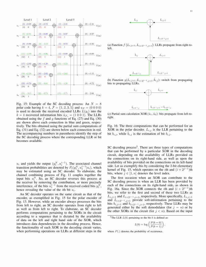
Fig. 15: Example of the SC decoding process: An N = 8polar code having k = 4, F = {1, 2, 3, 5} and uF = (0 0 0 0)is used to decode the received encoded LLRs L(yi) into thek = 4 recovered information bits uFc = (1 0 0 1). The LLRsobtained using the f and g functions of Eq. (27) and Eq. (30)are shown above each connection in blue and green, respec-tively. The bits obtained using the partial sum computations ofEq. (31) and Eq. (32) are shown below each connection in red.The accompanying numbers in parenthesis identify the step ofthe SC decoding process where the corresponding LLR or bitbecomes available.

ui and yields the output (yN1 , ui−1i ). The associated channel

transition probabilities are denoted by Pi(yN1 , ui−11 |ui), which

may be estimated using an SC decoder. To elaborate, thechannel combining process of Fig. 11 couples together theinput bits uNi . So, an SC decoder reverses this process atthe receiver by removing the contribution, or more preciselyinterference, of the bits ui−11 from the received coded bits yN1 ,hence revealing the value of the ith bit ui.

An SC decoder operates on the same circuit as that of theencoder, as exemplified in Fig. 15 for the polar encoder ofFig. 13. However, while an encoder always processes the bitsfrom left to right, an SC decoder operates from right to leftas well as from left to right. To elaborate, an SC decoderperforms computations pertaining to the XORs in the circuitaccording to a sequence that is dictated by the availabilityof data on the left and right hand side of the XOR, whichintroduces data dependencies in the decoding process. Hence,the functionality of each XOR in the decoding circuit varies,when performing operations on LLRs at different steps in the

Li,j+1

Li+2j−1,j+1

Li,j

(a) Function f(Li,j+1, Li+2j−1,j+1

): LLRs propagate from right-to-

left.

Li,j+1

Li+2j−1,j+1Li+2j−1,j

bi,j

(b) Function g(Li,j+1, Li+2j−1,j+1, bi,j): switch from propagatingbits to propagating LLRs.

bi,j+1

bi+2j−1,j+1 = bi+2j−1,jbi+2j−1,j

bi,j

(c) Partial sum calculation XOR (u1, u2): bits propagate from left-to-right.

Fig. 16: The three computations that can be performed for anXOR in the polar decoder. Li,j is the LLR pertaining to thebit bi,j , while bi,j is the estimation of bit bi,j .

SC decoding process5. There are three types of computationsthat can be performed by a particular XOR in the decodingcircuit, depending on the availability of LLRs provided onthe connections on its right-hand side, as well as upon theavailability of bits provided on the connections on its left-handside. Let us exemplify this by considering the 2-bit elementarykernel of Fig. 15, which operates on the ith and (i+ 2j−1)thbits, where j ∈ [1, n] denotes the level index.

The first occasion when an XOR can contribute to theSC decoding process is when an LLR has been provided byeach of the connections on its right-hand side, as shown inFig. 16a. Since the XOR connects the ith and (i + 2j−1)thbits, we refer to the first and second of these two LLRs asLi,j+1 and Li+2j−1,j+1, respectively. More specifically, Li,j+1

and Li+2j−1,j+1 provide soft-information pertaining to thebits bi,j+1 and bi+2j−1,j+1, respectively. These LLRs may begenerated either by the soft demodulator (for j = n) or bythe other XORs in the circuit (for j < n). Based on the input

5The LLR L(b) pertaining to the bit b is defined as:

L(b) = log

(P (b = 0)

P (b = 1)

),

where P (.) denotes the probability of occurrence.

12

Li,j+1 and Li+2j−1,j+1, the XOR of Fig. 16a computes theLLR Li,j for the first of the two connections on its left-handside, as follows:

Li,j = f(Li,j+1, Li+2j−1,j+1

)

= Li,j+1 � Li+2j−1,j+1, (27)

where the box-plus operator is defined as [128]:

L(b1)� L(b2)

= L(b1 ⊕ b2)

= ln1 + eL(b1)eL(b2)

eL(b1) + eL(b2)

= 2 tanh−1(tanh(L(b1)/2) tanh(L(b2)/2)) (28)= sign(L(b1))sign(L(b2))min(|L(b1)|, |L(b2)|)+ log

(1 + e−|L(b1)+L(b2)|

)− log

(1 + e−|L(b1)−L(b2)|

)

≈ sign(L(b1))sign(L(b2))min(|L(b1)|, |L(b2)|). (29)

Here, L(b1) and L(b2) are the LLRs pertaining to the bits b1and b2, respectively. The sign(·) of Eq. (29) returns −1 if itsargument is negative and +1 if its argument if positive. Here,Eq. (29) is referred to as the min-sum approximation.

Later in the SC decoding process, the estimated bit bi,jis provided on the first of the connections on the left-handside of the XOR, as shown in Fig. 16b. Together with theLLRs Li,j+1 and Li+2j−1,j+1 that were previously providedusing the connections on the right-hand side, this enables theXOR to compute the LLR Li+2j−1,j for the second of the twoconnections on its left-hand side, according to the g functionas follows:

Li+2j−1,j = g(Li,j+1, Li+2j−1,j+1, bi,j)

= (−1)bi,jLi,j+1 + Li+2j−1,j+1. (30)

We may observe in Eq. (30) that the g function is analogous tothe decoding operation of a repetition node, since the two LLRvalues are summed together. This is because the informationpertaining to the bit bi+2j−1,j is contained in Li+2j−1,j+1 aswell as in Li,j+1. Furthermore, the sign of Li,j+1 is flippedwhen bi,j = 1, since we have bi+2j−1,j = bi,j+1 ⊕ bi,j .

Later still, the bit bi+2j−1,j will be provided on the secondof the connections on the left-hand side of the XOR, as shownin Fig. 16c. Together with the bit bi,j that was previouslyprovided using the first of the connections on the left-handside, this enables the partial sum computation of bits bi,j+1

and bi+2j−1,j+1 for the first and second connections on theright-hand side of the XOR, where

bi,j+1 = XOR(bi,j , bi+2j−1,j), (31)

bi+2j−1,j+1 = bi+2j−1,j . (32)

As may be appreciated from the discussions above, thef function of Eq. (27) may be used to propagate LLRsfrom right-to-left within the SC decoder, while the partialsum computations of Eq. (31) and Eq. (32) may be used topropagate bits from left-to-right and the g function of Eq. (30)

may be used to switch from propagating bits from left-to-right to propagating LLRs from right-to-left. The SC decodingprocess begins by processing LLRs from right to left. However,in order that LLRs can be propagated from right to left, it isnecessary to provide LLRs on the connections on the right-hand edge of the circuit, i.e. right-hand connections at level3 of Fig. 15. In the example of Fig. 15, this is performed atthe start of the SC decoding process by providing successiveLLRs from a soft demodulator on successive connections onthe right-hand edge of the circuit. We may also call themchannel LLRs, since they provide soft information pertainingto the channel outputs. The SC decoding process then beginsby using the f function of Eq. (27) to propagate LLRs from theright hand edge of the decoding circuit to the top connectionon the left-hand edge, allowing the first bit to be recovered(steps (0) to (4) in Fig. 15). Explicitly, if the first bit is aninformation bit, then a hard-decision is made based on theresulting LLR L1,1. By contrast, if the first bit is a frozen bit,then it is set equivalent to the known frozen bit. Then the gfunction of Eq. (30) is used to compute the LLR pertainingto the second bit, hence revealing its value (steps (5) and (6)in Fig. 15). Following this, each successive bit from top tobottom is recovered by using the partial sum computationsof Eq. (31) and Eq. (32) to propagate bits from left to right,then using the g function of Eq. (30) for a particular XOR toswitch from bit propagation to LLR propagation, before usingthe f function to propagate LLRs to the next connection onthe left-hand edge of the circuit, allowing the correspondingbit to be recovered. It is pertinent to mention here that if bit onthe left-hand edge is a frozen bit, then the associated the LLRis ignored and the value of the bit is set to the known valueof the frozen bit. The complexity of this decoding process ison the order of O(N log2N), since there are n = log2Nlevels and each level invokes N/2 XOR gates. Furthermore, astraightforward implementation of the SC decoder also has achip-area proportional to O(N log2N), which was reduced toO(N) in [70] by exploiting the recursive nature of polar codesin conjunction with ‘lazy-copy’ algorithmic techniques.

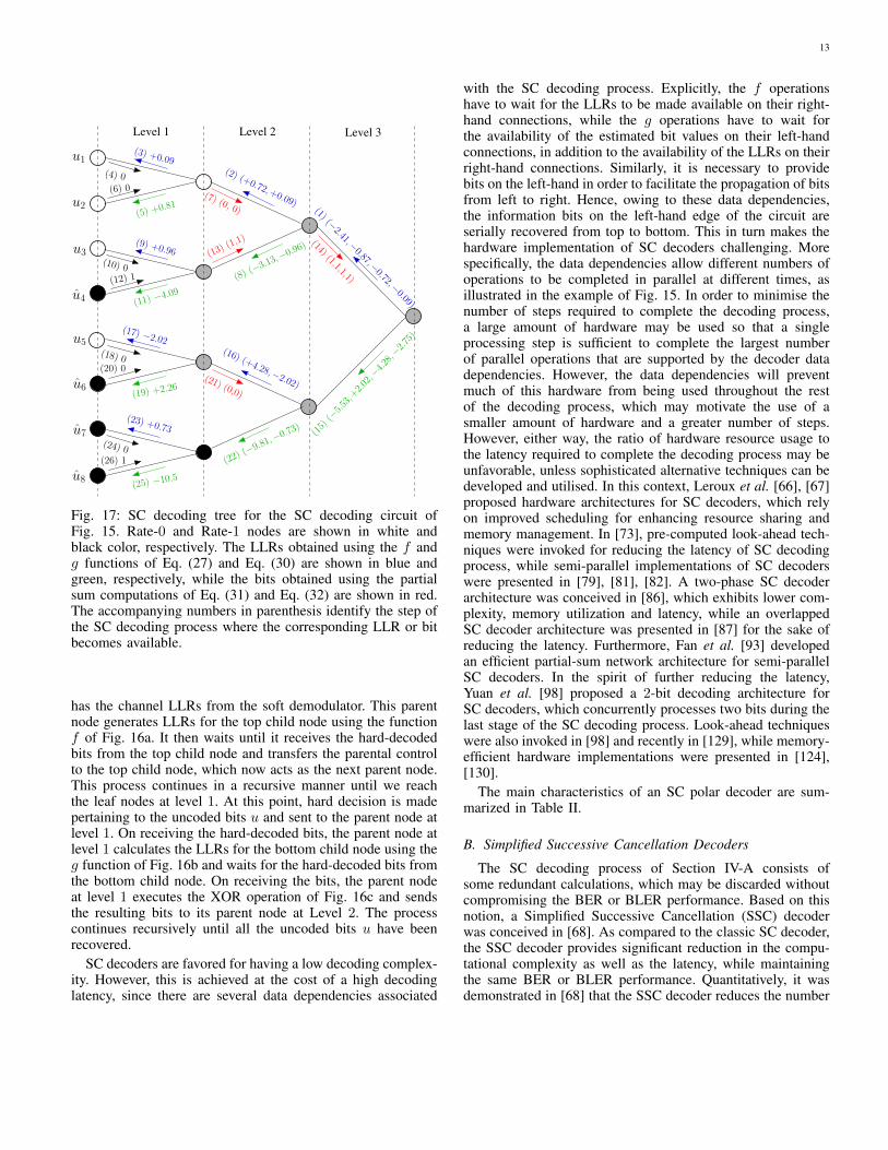
The SC decoding process of Fig. 15 may also be visualizedover a decoding tree, as shown in Fig. 17. The decoding tree ofFig. 17 consists of n = 3 levels and each level is composed of2n−i parent nodes and 2n−i+1 child nodes; hence resulting in23 = 8 leaf nodes at level 1, which correspond to the bits u. Toelaborate, the number of child nodes at each level correspondsto the number of distinct polarized channels created at thatlevel. Recall from Section II that we get two types of polarizedchannels W− and W+ at level 3, which are further polarizedinto W−−, W−+, W+− and W++ at level 2 and then intoeight types at level 1. This results in 2n−i+1 types of polarizedchannels at each level. Furthermore, the decoding tree at level3 starts with a length N parent node, whose length reducesby half at every child node, hence adopting a recursive divide-and-conquer approach.

Let us now elaborate on the flow of LLRs and bits throughthe decoding tree of Fig. 17, where each node acts as a localdecoder executing the XOR operations of Fig. 16. The SCdecoding process begins with the parent node at Level 3, which

13

Level 1 Level 3Level 2

(4) 0

(18) 0(20) 0

(24) 0(26) 1

u1

u2

u3

u4

u5

u6

u7

u8

(1) (−2.41,−

0.87,−0.72,−

0.09)

(2) (+0.72,+0.09)(5) +

0.81

(6) 0

(3) +0.09

(7) (0, 0)

(8)(−3.

13,−0.9

6)(9) +0.96

(10) 0

(11)−4.09

(12) 1

(13) (1

,1) (14) (1,1,1,1)

(15)(−5.53,+2.02,−4.28,−2.75)

(16) (+4.28,−2.02)

(17) −2.02

(19) +2.26(21) (0,0)

(22) (−

9.81,−0

.73)

(23) +0.73

(25) −10.5

Fig. 17: SC decoding tree for the SC decoding circuit ofFig. 15. Rate-0 and Rate-1 nodes are shown in white andblack color, respectively. The LLRs obtained using the f andg functions of Eq. (27) and Eq. (30) are shown in blue andgreen, respectively, while the bits obtained using the partialsum computations of Eq. (31) and Eq. (32) are shown in red.The accompanying numbers in parenthesis identify the step ofthe SC decoding process where the corresponding LLR or bitbecomes available.

has the channel LLRs from the soft demodulator. This parentnode generates LLRs for the top child node using the functionf of Fig. 16a. It then waits until it receives the hard-decodedbits from the top child node and transfers the parental controlto the top child node, which now acts as the next parent node.This process continues in a recursive manner until we reachthe leaf nodes at level 1. At this point, hard decision is madepertaining to the uncoded bits u and sent to the parent node atlevel 1. On receiving the hard-decoded bits, the parent node atlevel 1 calculates the LLRs for the bottom child node using theg function of Fig. 16b and waits for the hard-decoded bits fromthe bottom child node. On receiving the bits, the parent nodeat level 1 executes the XOR operation of Fig. 16c and sendsthe resulting bits to its parent node at Level 2. The processcontinues recursively until all the uncoded bits u have beenrecovered.

SC decoders are favored for having a low decoding complex-ity. However, this is achieved at the cost of a high decodinglatency, since there are several data dependencies associated

with the SC decoding process. Explicitly, the f operationshave to wait for the LLRs to be made available on their right-hand connections, while the g operations have to wait forthe availability of the estimated bit values on their left-handconnections, in addition to the availability of the LLRs on theirright-hand connections. Similarly, it is necessary to providebits on the left-hand in order to facilitate the propagation of bitsfrom left to right. Hence, owing to these data dependencies,the information bits on the left-hand edge of the circuit areserially recovered from top to bottom. This in turn makes thehardware implementation of SC decoders challenging. Morespecifically, the data dependencies allow different numbers ofoperations to be completed in parallel at different times, asillustrated in the example of Fig. 15. In order to minimise thenumber of steps required to complete the decoding process,a large amount of hardware may be used so that a singleprocessing step is sufficient to complete the largest numberof parallel operations that are supported by the decoder datadependencies. However, the data dependencies will preventmuch of this hardware from being used throughout the restof the decoding process, which may motivate the use of asmaller amount of hardware and a greater number of steps.However, either way, the ratio of hardware resource usage tothe latency required to complete the decoding process may beunfavorable, unless sophisticated alternative techniques can bedeveloped and utilised. In this context, Leroux et al. [66], [67]proposed hardware architectures for SC decoders, which relyon improved scheduling for enhancing resource sharing andmemory management. In [73], pre-computed look-ahead tech-niques were invoked for reducing the latency of SC decodingprocess, while semi-parallel implementations of SC decoderswere presented in [79], [81], [82]. A two-phase SC decoderarchitecture was conceived in [86], which exhibits lower com-plexity, memory utilization and latency, while an overlappedSC decoder architecture was presented in [87] for the sake ofreducing the latency. Furthermore, Fan et al. [93] developedan efficient partial-sum network architecture for semi-parallelSC decoders. In the spirit of further reducing the latency,Yuan et al. [98] proposed a 2-bit decoding architecture forSC decoders, which concurrently processes two bits during thelast stage of the SC decoding process. Look-ahead techniqueswere also invoked in [98] and recently in [129], while memory-efficient hardware implementations were presented in [124],[130].

The main characteristics of an SC polar decoder are sum-marized in Table II.

B. Simplified Successive Cancellation Decoders

The SC decoding process of Section IV-A consists ofsome redundant calculations, which may be discarded withoutcompromising the BER or BLER performance. Based on thisnotion, a Simplified Successive Cancellation (SSC) decoderwas conceived in [68]. As compared to the classic SC decoder,the SSC decoder provides significant reduction in the compu-tational complexity as well as the latency, while maintainingthe same BER or BLER performance. Quantitatively, it wasdemonstrated in [68] that the SSC decoder reduces the number

14

Complexity • Time complexity = O(N log2N)• Space complexity = O(N)

Advantages • Low decoding complexity• Asymptotically capacity achieving

Disadvantages • Sub-optimal finite-length performance• Serial processing, resulting in high latency (or low throughput)• Fully-parallel implementation not feasible

TABLE II: Main characteristics of an SC polar decoder.

of computationally intensive box-plus operators of Eq. (28) byaround 20% to 50%, while the decoding latency is reduced byaround 75% to 95%.

The SSC decoder exploits the tree structure of Fig. 17 fordiscarding redundant computations. Explicitly, the nodes ofFig. 17 may be classified into three types, as follows:

1) Rate-0 nodes, whose descendants are all frozen bits(white nodes in Fig. 17);

2) Rate-1 nodes, whose descendants are all informationbits (black nodes in Fig. 17);

3) Rate-R nodes, whose descendants are a mix of frozenbits and information bits (gray nodes in Fig. 17).

Recall that the value of frozen bits may be directly used atthe decoder rather than estimating it based on the computedLLRs. Consequently, the SSC decoder de-activates the f andg operations at Rate-0 nodes of Fig. 17 without affecting thedecoder’s performance. Explicitly, u1 and u2 are initialized tothe known value of frozen bits, i.e. 0, in the SSC decoder, andsteps (3) to (6) are not required. Similarly, the SSC decoderfurther reduces the complexity at the Rate-1 nodes by makinga hard-decision based on the input LLRs and passing thehard-decoded bits to the child nodes, rather than computingthe f and g functions. In the context of Fig. 17, an SSCdecoder makes hard-decision based on the LLRs computedin step (22) revealing u8, discards steps (23) to (26), andestimates u7 based on the hard-decision values of step (22).Since all nodes connected to the Rate-1 nodes are informationbits, this simplification does not affect the performance of thedecoder. Improved versions of the SSC decoder were proposedin [80], [88] for the sake of further reducing the associatedlatencies, while the hardware architectures of SSC decoderwere presented in [88], [95].

The main characteristics of an SSC polar decoder aresummarized in Table III.

C. Successive Cancellation List (SCL) Decoders

The SC decoder provably achieves the capacity of a B-DMC,when the codeword length is infinitely long. However, itdoes not exhibit good performance at finite codeword lengths,because the channels are not sufficiently polarized. Morespecifically, in the SC decoding process, the value of each

Complexity Depends on the underlying polar code

Advantages • Lower complexity and latency than SC• Asymptotically capacity achieving

Disadvantages • Sub-optimal finite-length performance• Serial processing, resulting in high latency (or low throughput)• Fully-parallel implementation not feasible

TABLE III: Main characteristics of an SSC polar decoder.

recovered information bit ui depends on all the previous recov-ered information bits ui−11 . Consequently, if a bit is incorrectlydecoded, it will often catastrophically propagate the errors toall subsequent bits. The selection of an incorrect value foran information bit may be detected with consideration of thesubsequent frozen bits, since the decoder knows that these bitsshould have values of 0. More specifically, if the correspondingLLR has a sign that would imply a value of 1 for a frozen bit,then this suggests that an error may have been made during thedecoding of one of the preceding information bits. However,in the SC decoding process, there is no opportunity to consideralternative values for the preceding information bits. Once avalue has been selected for an information bit, the SC decodingprocess moves on and the decision is final.

Inspired by the recursive list decoding of RM codes [131],Tal and Vardy proposed an LR-based SCL decoder [69],[70], whose LLR-based counterpart was presented in [101].In contrast to an SC decoder, an SCL decoder considers a listof alternative values for the information bits, hence improvingthe finite-length performance of polar codes. More explicitly,as the decoding process progresses, an SCL decoder considersboth options for the value of each successive information bit,rather than making a hard-decision based on the associatedLLR value. This is achieved by maintaining a list of candi-date information bits, where the list is built up as the SCLdecoding proceeds. At the start of the process, the list isempty. Whenever the decoding process reaches a frozen bit,a bit value of 0 is appended to the list. However, wheneverthe decoding process reaches an information bit, two replicasof the list are created. Here, the bit value of 0 is appendedto the first replica, while the bit value of 1 is appendedto the second replica. Hence, the number of lists, or morespecifically the number of candidate decoding paths, doubleswhenever an information bit is encountered. This continuesuntil the number of decoding paths reaches a limit L, whichis known as the list size and is typically chosen as a powerof two. From this point onwards, each time the number ofdecoding paths is doubled when considering an informationbit, the worst L amongst the 2L candidate paths are identifiedand pruned from the list. In this way, the size of the list ismaintained at L until the SCL decoding process completes. Astraightforward implementation of the SCL algorithm incurs acomplexity polynomial in the codeword length N . However,Tal and Vardy [70] exploited the recursive nature of polar codes

15

Level 1 Level 2 Level 3

(4) 0

(20) 0

(24) 0

(26) 1

(18) 0

(2) +0.72

(2) +0.09

(9) +0.96 (8) −3.13

(11) −4.09 (8) −0.96

(17) −2.02 (16) +4.28

(19) +2.26 (16) −2.02

(23) +0.73 (22) −9.81

(25) −10.5 (22) −0.73

(0) +2.41

(0) −0.87

(0) +3.56

(0) +0.09

(0) −3.12

(0) +1.15

(0) −0.72

(0) −2.66

(1) −0.72

(1) −0.09

(15) −5.53

(15) +2.02

(15) −4.28

(15) −2.75

L(y1)

L(y2)

L(y3)

L(y7)

u2

u3

u5

u4

u6

u7

u8

L(y6)

L(y4)

L(y5)

L(y8)

(1) −0.87

(1) −2.41

(5) +0.81

(3) +0.09

(7) 0

(6) 0 (7) 0

(10) 0 (13) 1

(13) 1(12) 1

(14) 1

(14) 1

(14) 1

(14) 1

(21) 0

(21) 0

u1

(12) 0 (13) 0

(13) 0

(14) 0

(14) 0

(14) 0

(14) 0

(15) −0.71

(15) +0.28

(15) +2.84

(15) −2.57

(16) −0.71

(16) −0.28

(17) +0.28

(18) 0(19) −0.99

(20) 1

(21) 1

(21) 1

(22) +3.55

(22) −2.85

(23) −2.85

(24) 1(25) −6.4

(26) 1

(a) An SCL (L = 2) decoding circuit. For the first candidate path, theLLRs obtained using the f and g functions of Eq. (27) and Eq. (30)are shown above each connection in blue and green, respectively, whilethe bits obtained using the partial sum computations of Eq. (31) andEq. (32) are shown below each connection in red. All the LLRs andbits pertaining to the second candidate path are shown in brown.The accompanying numbers in parenthesis identify the step of theSC decoding process where the corresponding LLR or bit becomesavailable.

X

X

X

X

X

0.0

0.0

0.0

0.04.09

4.09 2.02

4.09 2.02

u7

u8

u6

u5

u4

u3

u2

u1

6.94 4.09 2.02 2.75

2.02 2.75

ui = 0ui = 1

12.52

9.15

4.285.08

(b) SCL decoding over a binary tree. Frozen and information nodesare marked in red and black, respectively, the two candidate paths areshown in green and brown, and the pruned paths are marked with a redcross. The values next to the branches are the associated path metricscomputed using Eq. (34). Please note that the green path is the same asthe SC decoding path.

Fig. 18: Example of an SCL decoding process (L = 2): An N = 8 polar code having k = 4, F = {1, 2, 3, 5} and uF = (0 0 0 0)is used to decode the received encoded LLRs L(yi) into the k = 4 recovered information bits uFc = (1 0 0 1).

together with ‘lazy-copy’ algorithmic techniques to reduce thetime complexity to O(LN log2N) and the space complexityto O(LN), both of which are L times the complexities of theclassic SC decoder.

The SCL decoding process may be viewed as a path searchin a binary tree of depth N , as illustrated in Fig. 18b forthe decoding circuit of Fig. 18a. The input bits ui may besuccessively recovered as we move down the binary tree.Explicitly, the nodes of the binary tree (except for the leafnodes) of Fig. 18b correspond to the input ui, while thebranches represent the possible values 0 and 1 of the bit ui.Consequently, all the information nodes (marked in black inFig. 18) have two branches, while the frozen nodes (markedin red in Fig. 18) have a single branch, since their values areknown to the decoder. The lth branch at depth i ∈ [1, N ]is identified with a path metric φl,i, which is calculated as

follows:

φl,i = φl,i−1 + ln(1 + e−(1−2ul,i)L(ul,i)) (33)

≈{φl,i−1 if ul,i = 1

2 (1− sign(L(ul,i)))φl,i−1 + |L(ul,i)| otherwise ,

(34)

where φl,i−1 is the parent path’s metric at depth (i− 1), ul,iis the value of ui associated with the lth branch and L(ul,i)denotes the corresponding LLR Li,1 obtained on the left-handedge of the polar decoding circuit of Fig. 18a. These LLRsare obtained throughout the SCL decoding process by usingseparate replicas of the partial sum computations of Eq. (31)and Eq. (32) to propagate the bits of each candidate pathfrom left to right. Similarly, separate replicas of the f andg computations of Eq. (27) and Eq. (30) are used to propagatecorresponding replicas of the LLRs, as shown in Fig. 18a inbrown color for the second candidate path. Here, Eq. (34) isreferred to as the min-sum approximation. Intuitively, Eq. (34)implies that if the value of bit ul,i corresponding to the branch

16

-1 0 1 2 3 4

Eb/N

0 [dB]

10-4

10-3

10-2

10-1

100

BL

ER

L=1

L=2

L=4

L=8

L=16

L=32

Fig. 19: The achievable BLER performance of the SCLdecoder for variable list sizes. A (1024, 512) polar coderelying on the 5G frozen bit sequence was used in conjunctionwith QPSK transmission over an AWGN channel. Min-sumapproximation of Eq. (29) was invoked for calculating box-plus operations.

at depth i complies with the LLR L(ul,i), then the pathmetric is left unchanged, otherwise it is penalized by |L(ul,i)|.Furthermore, Eq. (34) accumulates across all bit positionsi ∈ [1, N ]. So, it must be calculated for all L candidate pathswhenever a frozen bit value of 0 is appended, as well as forall 2L candidates when both possible values of an informationbit are considered. In the latter case, the 2L metrics are sortedand the L candidates having the highest values are identifiedas being the worst and are pruned from the list, as shown inFig. 18b for L = 2. Following the completion of the SCLdecoding process, the candidate path having the lowest metricmay be selected as the most likely decoding path. It is pertinentto mention here that an SCL decoder having L = 1 is the sameas an SC decoder and it becomes equivalent to a MaximumLikelihood (ML) decoder, when L = 2k, implying a searchthrough all possible 2k codewords.

Fig. 19 records the BLER performance of the SCL decoderfor variable list sizes L. We may observe in Fig. 19 thatthe BLER performance improves upon increasing the valueof L, providing significant improvement over the SC decoder(L = 1). However, the performance improves with diminishingreturns at higher values of L. More precisely, the performanceimprovement is only marginal for L > 8. Hence, a list sizeof 8 is deemed sufficient, while a list size of 32 brings theperformance arbitrary close to that of the ML decoder, asdemonstrated in [70].

Despite the improved performance of the SCL decoder,polar codes failed to outperform the state-of-the-art LDPCand turbo codes [70], which may be attributed to their poor

minimum distance. More specifically, the authors of [74] ob-served that when the SCL decoder failed to output the correctinformation sequence, the correct information sequence wasusually present in its list of candidate paths, but with a smallerpath metric. This motivated the development of the CyclicRedundancy Check-Aided SCL (CA-SCL) decoder [70], [74],while an adaptive CA-SCL decoding scheme was developedin [75]. The Cyclic Redundancy Check (CRC)-aided approachconcatenates a CRC to the polar code as an outer code, sothat a portion of the information bits is utilized for carryingthe CRC bits. More specifically, (k − r) information bitsare first encoded using a CRC code, which appends an r-bit CRC to the (k − r) information bits. This CRC code cansimply be a small random systematic linear block code. Theresulting CRC encoded bits are then passed to the inner polarcode. At the CA-SCL decoder, all candidate paths that donot satisfy the CRC are pruned during the last stage of theclassic SCL decoding process, before the candidate having thelowest metric is selected as the most likely decoding path. TheCA-SCL decoder improved the performance of polar codesto be on par with the state-of-the-art turbo and LDPC codes,while retaining the complexity of the classic SCL decoder.However, this is achieved at the cost of a small loss in thecoding rate, since the coding rate of the resultant concatenatedcode is (k − r)/N . The notion of CRC-aided concatenationwas generalized to parity check codes in [116].

In pursuit of approaching the perfromance of the SCLdecoder with the SC decoder’s space requirements, bit-flipdecoding strategy was adopted in [99]. The proposed SC flipdecoder of [99] enhances the performance of the classic SCdecoder by exploiting CRC in conjunction with the bit-flippingalgorithm. More specifically, the SC flip decoder commencesthe decoding process by running a single iteration of the classicSC decoder for estimating the codeword u, as exemplifiedin Fig. 15. If the CRC passes with the estimated codewordu, the decoding process is terminated. Otherwise, upto Tadditional SC decoding iterations are invoked, sequentiallyflipping the estimated value of one of the T least reliablebits in each iteration. The process is repeated until the CRCpasses or the maximum number of attempts T is reached.While the SC flip decoder preserves the space requirementsof the classic SC decoder as well as improves the decodingperformance, it fails to outperform the SCL decoder, sincethe bit-flip algorithm is only capable of correcting a singleadditional error. Furthermore, the computational complexity issubstantially high at low SNRs and approaches that of the SCdecoder at high SNRs. Improvements to the SC flip decoderwere proposed in [132]–[134], while the use of the bit-flipalgorithm was extended to the SSC and the SCL decodersin [125], [135] and [136].

Similarly to the classic SC decoder, the SCL decodingscheme also suffers from a high latency due to the datadependencies associated with the decoding process. In thiscontext, various low-latency SCL decoding schemes have beenpresented in [94], [104], [105], [108], [110], [111], [117].Furthermore, the complexity of an SCL decoder is L timeshigher than that of a classic SC decoder, since it processes L

17

Complexity • Time complexity = O(LN log2N)• Space complexity = O(LN)

Advantages • Capable of achieving the ML performance• Performance of CA-SCL is on par with turbo and LDPC codes

Disadvantages • Serial processing, resulting in high latency (or low throughput)• Fully-parallel implementation not feasible• Higher complexity than SC• Higher latency than SC due to the ‘metric sorting’ operation

TABLE IV: Main characteristics of an SCL polar decoder.

candidate paths. For the sake of reducing the complexity ofSCL decoders, reduced-complexity techniques were exploredin [112], [114]. Another key challenge in the SCL decodingprocess is imposed by metric sorting, which is required toidentify the worst L candidate paths among the merged listof 2L paths for pruning. Simultaneously comparing all the2L path metrics requires large amount of hardware resources,while successively comparing the paths increases the latency.Hence, a suitable compromise must be reached between therequired hardware resources and the imposed latency. Hard-ware implementations of the SCL decoder have been discussedin [91], [94], [101]–[103], [109], [113], [115], [117], [121],[124], [127], while an unsorted SCL decoder was conceivedin [118].

The main characteristics of an SCL polar decoder aresummarized in Table IV.

D. Successive Cancellation Stack (SCS) Decoders

The SC decoding may be viewed as a greedy search over thebinary tree of Fig. 18b, since it only considers the path with thelowest metric, hence making a bit-by-bit decision. By contrast,the SCL decoding adopts a breadth-first approach, doubling thenumber of paths for each information bit and selecting the bestL paths for further processing. The breadth-first approach ofSCL provides attractive performance benefits at the cost of anincreased computational complexity, because L paths have tobe processed in contrast to the single decoding path of SC.For the sake of achieving a reasonable compromise betweenthe performance and computational complexity, SuccessiveCancellation Stack (SCS) decoding was proposed in [72] ,inspired by the stack decoding of convolutional codes [137]and RM codes [138].

Similarly to SCL decoding, SCS decoding also operates overthe binary tree of Fig. 18b. However, while an SCL decoderrecords the L best candidate paths (having the lowest pathmetric) of the same length, an SCS decoder records the Dbest candidate paths of variable lengths in an ordered stack.Furthermore, in contrast to the SCL decoding, which processesall the L candidate paths in parallel, SCS decoding onlyprocesses the path at the top of the stack at a time, hencereducing the computational complexity. Let us elaborate on

this by revisiting the decoding example of Fig. 18 with theSSC algorithm.

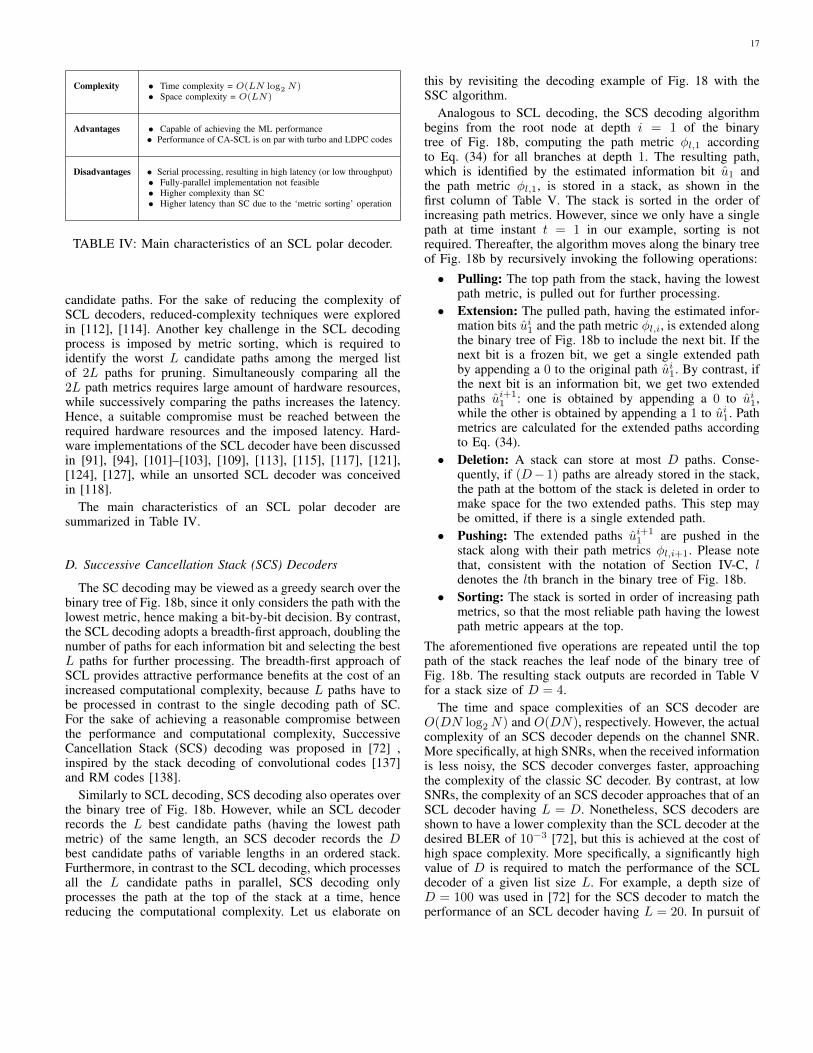
Analogous to SCL decoding, the SCS decoding algorithmbegins from the root node at depth i = 1 of the binarytree of Fig. 18b, computing the path metric φl,1 accordingto Eq. (34) for all branches at depth 1. The resulting path,which is identified by the estimated information bit u1 andthe path metric φl,1, is stored in a stack, as shown in thefirst column of Table V. The stack is sorted in the order ofincreasing path metrics. However, since we only have a singlepath at time instant t = 1 in our example, sorting is notrequired. Thereafter, the algorithm moves along the binary treeof Fig. 18b by recursively invoking the following operations:

• Pulling: The top path from the stack, having the lowestpath metric, is pulled out for further processing.

• Extension: The pulled path, having the estimated infor-mation bits ui1 and the path metric φl,i, is extended alongthe binary tree of Fig. 18b to include the next bit. If thenext bit is a frozen bit, we get a single extended pathby appending a 0 to the original path ui1. By contrast, ifthe next bit is an information bit, we get two extendedpaths ui+1

1 : one is obtained by appending a 0 to ui1,while the other is obtained by appending a 1 to ui1. Pathmetrics are calculated for the extended paths accordingto Eq. (34).

• Deletion: A stack can store at most D paths. Conse-quently, if (D−1) paths are already stored in the stack,the path at the bottom of the stack is deleted in order tomake space for the two extended paths. This step maybe omitted, if there is a single extended path.

• Pushing: The extended paths ui+11 are pushed in the

stack along with their path metrics φl,i+1. Please notethat, consistent with the notation of Section IV-C, ldenotes the lth branch in the binary tree of Fig. 18b.

• Sorting: The stack is sorted in order of increasing pathmetrics, so that the most reliable path having the lowestpath metric appears at the top.

The aforementioned five operations are repeated until the toppath of the stack reaches the leaf node of the binary tree ofFig. 18b. The resulting stack outputs are recorded in Table Vfor a stack size of D = 4.

The time and space complexities of an SCS decoder areO(DN log2N) and O(DN), respectively. However, the actualcomplexity of an SCS decoder depends on the channel SNR.More specifically, at high SNRs, when the received informationis less noisy, the SCS decoder converges faster, approachingthe complexity of the classic SC decoder. By contrast, at lowSNRs, the complexity of an SCS decoder approaches that of anSCL decoder having L = D. Nonetheless, SCS decoders areshown to have a lower complexity than the SCL decoder at thedesired BLER of 10−3 [72], but this is achieved at the cost ofhigh space complexity. More specifically, a significantly highvalue of D is required to match the performance of the SCLdecoder of a given list size L. For example, a depth size ofD = 100 was used in [72] for the SCS decoder to match theperformance of an SCL decoder having L = 20. In pursuit of

18

t = 1 t = 2 t = 3 t = 4 t = 5 t = 6 t = 7 t = 8

u1 φ1,1 = 0.0 u21 φ1,2 = 0.0 u3

1 φ1,3 = 0.0 u41 φ2,4 = 0.0 u5

1 φ2,5 = 2.02 u61 φ3,6 = 2.02 u7

1 φ5,7 = 2.02 u81 φ10,8 = 2.02

u41 φ1,4 = 4.09 u4

1 φ1,4 = 4.09 u41 φ1,4 = 4.09 u7

1 φ6,7 = 2.75 u71 φ6,7 = 2.75

u61 φ4,6 = 4.28 u4

1 φ1,4 = 4.09 u41 φ1,4 = 4.09

u61 φ4,6 = 4.28 u8

1 φ9,8 = 12.52

TABLE V: An example of the SCS decoding process (D = 4) corresponding to the SCL decoding example of Fig. 18. Eachcolumn records the stack outputs at time instant t. The deleted path is highlighted in red, while the final optimal path is markedin green.

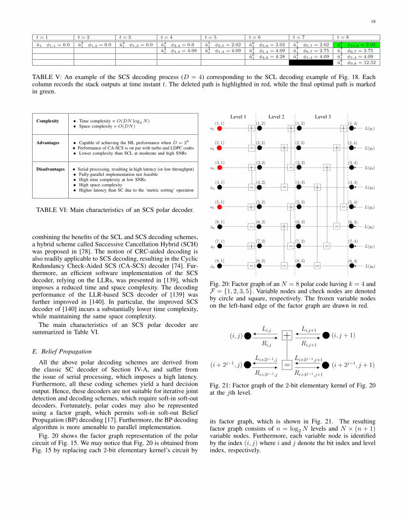
Complexity • Time complexity = O(DN log2N)• Space complexity = O(DN)

Advantages • Capable of achieving the ML performance when D = 2k

• Performance of CA-SCS is on par with turbo and LDPC codes• Lower complexity than SCL at moderate and high SNRs

Disadvantages • Serial processing, resulting in high latency (or low throughput)• Fully-parallel implementation not feasible• High time complexity at low SNRs• High space complexity• Higher latency than SC due to the ‘metric sorting’ operation

TABLE VI: Main characteristics of an SCS polar decoder.

combining the benefits of the SCL and SCS decoding schemes,a hybrid scheme called Successive Cancellation Hybrid (SCH)was proposed in [78]. The notion of CRC-aided decoding isalso readily applicable to SCS decoding, resulting in the CyclicRedundancy Check-Aided SCS (CA-SCS) decoder [74]. Fur-thermore, an efficient software implementation of the SCSdecoder, relying on the LLRs, was presented in [139], whichimposes a reduced time and space complexity. The decodingperformance of the LLR-based SCS decoder of [139] wasfurther improved in [140]. In particular, the improved SCSdecoder of [140] incurs a substantially lower time complexity,while maintaining the same space complexity.

The main characteristics of an SCS polar decoder aresummarized in Table VI.

E. Belief Propagation

All the above polar decoding schemes are derived fromthe classic SC decoder of Section IV-A, and suffer fromthe issue of serial processing, which imposes a high latency.Furthermore, all these coding schemes yield a hard decisionoutput. Hence, these decoders are not suitable for iterative jointdetection and decoding schemes, which require soft-in soft-outdecoders. Fortunately, polar codes may also be representedusing a factor graph, which permits soft-in soft-out BeliefPropagation (BP) decoding [17]. Furthermore, the BP decodingalgorithm is more amenable to parallel implementation.

Fig. 20 shows the factor graph representation of the polarcircuit of Fig. 15. We may notice that Fig. 20 is obtained fromFig. 15 by replacing each 2-bit elementary kernel’s circuit by

Level 1 Level 3Level 2

+

=

+

=

+

=

+

= =

=

+

+ +

+

+

+

=

=

+

+

=

=

=

=

L(y1)

L(y2)

L(y3)

L(y4)

L(y5)

L(y6)

L(y8)

L(y7)

(1, 1)

(2, 1)

(3, 1)

(4, 1)

(5, 1)

(6, 1)

(8, 1)

(1, 3)

(2, 3)

(3, 3)

(4, 3)

(5, 3)

(6, 3)

(8, 3)

(1, 4)

(2, 4)

(3, 4)

(4, 4)

(5, 4)

(6, 4)

(8, 4)

(1, 2)

(2, 2)

(3, 2)

(4, 2)

(5, 2)

(6, 2)

(8, 2)

u1

u2

u3

u4

u5

u6

u7

u8

(7, 1) (7, 2) (7, 3) (7, 4)

Fig. 20: Factor graph of an N = 8 polar code having k = 4 andF = {1, 2, 3, 5}. Variable nodes and check nodes are denotedby circle and square, respectively. The frozen variable nodeson the left-hand edge of the factor graph are drawn in red.

+

=

Ri,j

Li,j

Ri+2j−1,j

Li+2j−1,j

(i, j)

(i+ 2j−1, j)

(i, j + 1)

(i+ 2j−1, j + 1)Ri+2j−1,j+1

Li+2j−1,j+1

Ri,j+1

Li,j+1

Fig. 21: Factor graph of the 2-bit elementary kernel of Fig. 20at the jth level.

its factor graph, which is shown in Fig. 21. The resultingfactor graph consists of n = log2N levels and N × (n + 1)variable nodes. Furthermore, each variable node is identifiedby the index (i, j) where i and j denote the bit index and levelindex, respectively.

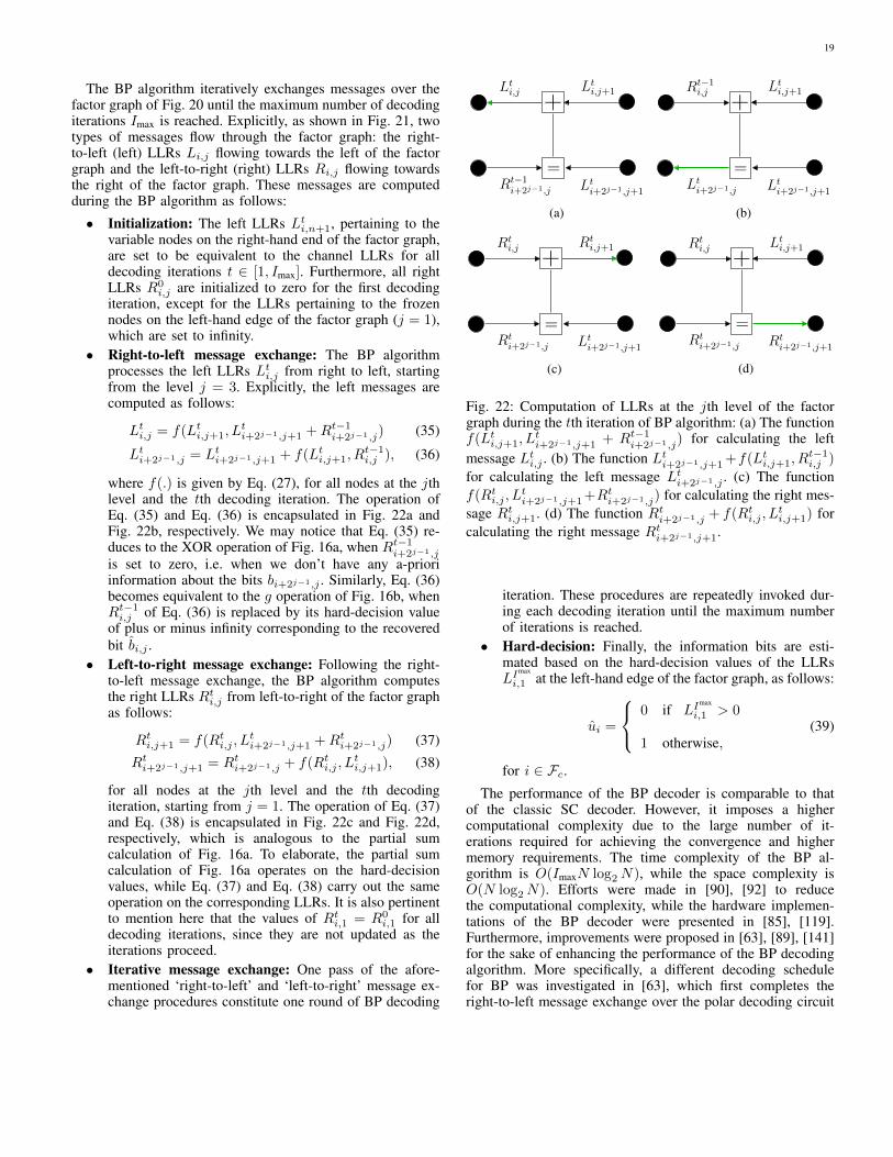
19

The BP algorithm iteratively exchanges messages over thefactor graph of Fig. 20 until the maximum number of decodingiterations Imax is reached. Explicitly, as shown in Fig. 21, twotypes of messages flow through the factor graph: the right-to-left (left) LLRs Li,j flowing towards the left of the factorgraph and the left-to-right (right) LLRs Ri,j flowing towardsthe right of the factor graph. These messages are computedduring the BP algorithm as follows:

• Initialization: The left LLRs Lti,n+1, pertaining to thevariable nodes on the right-hand end of the factor graph,are set to be equivalent to the channel LLRs for alldecoding iterations t ∈ [1, Imax]. Furthermore, all rightLLRs R0

i,j are initialized to zero for the first decodingiteration, except for the LLRs pertaining to the frozennodes on the left-hand edge of the factor graph (j = 1),which are set to infinity.

• Right-to-left message exchange: The BP algorithmprocesses the left LLRs Lti,j from right to left, startingfrom the level j = 3. Explicitly, the left messages arecomputed as follows:

Lti,j = f(Lti,j+1, Lti+2j−1,j+1 +Rt−1i+2j−1,j) (35)

Lti+2j−1,j = Lti+2j−1,j+1 + f(Lti,j+1, Rt−1i,j ), (36)

where f(.) is given by Eq. (27), for all nodes at the jthlevel and the tth decoding iteration. The operation ofEq. (35) and Eq. (36) is encapsulated in Fig. 22a andFig. 22b, respectively. We may notice that Eq. (35) re-duces to the XOR operation of Fig. 16a, when Rt−1i+2j−1,jis set to zero, i.e. when we don’t have any a-prioriinformation about the bits bi+2j−1,j . Similarly, Eq. (36)becomes equivalent to the g operation of Fig. 16b, whenRt−1i,j of Eq. (36) is replaced by its hard-decision valueof plus or minus infinity corresponding to the recoveredbit bi,j .

• Left-to-right message exchange: Following the right-to-left message exchange, the BP algorithm computesthe right LLRs Rti,j from left-to-right of the factor graphas follows:

Rti,j+1 = f(Rti,j , Lti+2j−1,j+1 +Rti+2j−1,j) (37)

Rti+2j−1,j+1 = Rti+2j−1,j + f(Rti,j , Lti,j+1), (38)

for all nodes at the jth level and the tth decodingiteration, starting from j = 1. The operation of Eq. (37)and Eq. (38) is encapsulated in Fig. 22c and Fig. 22d,respectively, which is analogous to the partial sumcalculation of Fig. 16a. To elaborate, the partial sumcalculation of Fig. 16a operates on the hard-decisionvalues, while Eq. (37) and Eq. (38) carry out the sameoperation on the corresponding LLRs. It is also pertinentto mention here that the values of Rti,1 = R0

i,1 for alldecoding iterations, since they are not updated as theiterations proceed.

• Iterative message exchange: One pass of the afore-mentioned ‘right-to-left’ and ‘left-to-right’ message ex-change procedures constitute one round of BP decoding

+

=Rt−1

i+2j−1,j Lti+2j−1,j+1

Lti,j Lt

i,j+1

(a)

+

=Lti+2j−1,j Lt

i+2j−1,j+1

Rt−1i,j Lt

i,j+1

(b)

+

=Rt

i+2j−1,j Lti+2j−1,j+1

Rti,j Rt

i,j+1

(c)

+

=Rt

i+2j−1,j Rti+2j−1,j+1

Rti,j Lt

i,j+1

(d)

Fig. 22: Computation of LLRs at the jth level of the factorgraph during the tth iteration of BP algorithm: (a) The functionf(Lti,j+1, L

ti+2j−1,j+1 + Rt−1i+2j−1,j) for calculating the left

message Lti,j . (b) The function Lti+2j−1,j+1+f(Lti,j+1, R

t−1i,j )

for calculating the left message Lti+2j−1,j . (c) The functionf(Rti,j , L

ti+2j−1,j+1+R

ti+2j−1,j) for calculating the right mes-

sage Rti,j+1. (d) The function Rti+2j−1,j + f(Rti,j , Lti,j+1) for

calculating the right message Rti+2j−1,j+1.

iteration. These procedures are repeatedly invoked dur-ing each decoding iteration until the maximum numberof iterations is reached.

• Hard-decision: Finally, the information bits are esti-mated based on the hard-decision values of the LLRsLI

max

i,1 at the left-hand edge of the factor graph, as follows:

ui =

0 if LImax

i,1 > 0

1 otherwise,(39)

for i ∈ Fc.The performance of the BP decoder is comparable to that

of the classic SC decoder. However, it imposes a highercomputational complexity due to the large number of it-erations required for achieving the convergence and highermemory requirements. The time complexity of the BP al-gorithm is O(ImaxN log2N), while the space complexity isO(N log2N). Efforts were made in [90], [92] to reducethe computational complexity, while the hardware implemen-tations of the BP decoder were presented in [85], [119].Furthermore, improvements were proposed in [63], [89], [141]for the sake of enhancing the performance of the BP decodingalgorithm. More specifically, a different decoding schedulefor BP was investigated in [63], which first completes theright-to-left message exchange over the polar decoding circuit

20

Complexity • Time complexity = O(ImaxN log2N)• Space complexity = O(N log2N)

Advantages • Soft output, hence compatible with iterative detection• Fully-parallel implementation

Disadvantages • Sub-optimal performance (better than SC)• High complexity• High memory requirements

TABLE VII: Main characteristics of a BP polar decoder.

and then proceeds with the left-to-right message exchange.An alternative technique was also investigated in [63], calledthe overcomplete representation (also called permuted factor-graph), which permutes the different levels of the polar factorgraph of Fig. 20 for achieving decoding convergence. In [89],the reliability of BP messages was improved by incorporatingthe knowledge of frozen bits, while a CRC was invoked in[141] together with the overcomplete representation of [63]for achieving decoding convergence. Despite these efforts, theBP algorithm did not outperform the SCL or SCS decoders.Recently, a BP list decoding algorithm was conceived in [126],which combines the benefits of the classic BP and SCLdecoders. Explicitly, the BP list decoder benefits from the gooderror correction capabilities of the SCL decoder and the soft-in soft-out nature of the classic BP algorithm. Furthermore,it also lends itself to parallel implementation, hence there isa possibility of achieving a lower latency. However, the BPlist decoder imposes a high computational complexity andits compatibility with CRC-aided polar codes needs to beinvestigated.

The main characteristics of a BP polar decoder are summa-rized in Table VII.

F. Soft Cancellation (SCAN)

The SC decoder of Section IV-A is a soft-in hard-outdecoder, since hard-decisions are made pertaining to the bitsbi,j during the decoding process. In the spirit of extracting softoutput from the SC decoder, a Soft CANcellation (SCAN)decoder was proposed [83], [84], which is in essence acombination of the SC decoder of Section IV-A and the BPdecoder of Section IV-E. Recall that the left-to-right messageexchange procedure of BP is a soft-valued version of the fand g operations of an SC decoder. Similarly, the right-to-leftmessage exchange of BP is a soft-valued counterpart of thepartial sum calculation of SC. Hence, we may conclude that alloperations of BP are soft-valued versions of the operations ofSC, but they follow a different processing schedule. A SCANdecoder combines the attributes of SC and BP decoding algo-rithms by using the BP operations of Fig. 22 in combinationwith the SC processing schedule. This in turn facilitates fasterconvergence of the resulting decoding algorithm, hence drasti-cally reducing the computational complexity. Quantitatively, it

Complexity • Time complexity = O(ImaxN log2N)• Space complexity = O(N log2N)

Advantages • Soft output, hence compatible with iterative detection• Much lower complexity than BP• Much lower memory requirements than BP

Disadvantages • Sub-optimal performance (better than SC)• Serial processing, resulting in high latency• Fully-parallel implementation not feasible

TABLE VIII: Main characteristics of a SCAN polar decoder.

-2 -1 0 1 2 3 4

Eb/N

0 [dB]

10-3

10-2

10-1

100

BL

ER

SC

BP Imax

=30

SCAN Imax

=5

SCL L=8

CA-SCL L=8, r=11

SCS D=128

Fig. 23: Comparison of the achievable BLER performanceof the polar decoders. A (1024, 512) polar code relying onthe 5G NR frozen bit sequence was used in conjunctionwith QPSK transmission over an AWGN channel. Min-sumapproximation of Eq. (29) was invoked for calculating the box-plus operations in all decoders, except in the BP decoder, forwhich the exact computation of Eq. (28) was used.

was demonstrated in [84] that the computational complexity ofthe SCAN decoder is only 4% of the complexity of the classicBP decoder. Another notable contribution in the context ofsoft-in soft-out polar decoders is the soft counterpart of theSCL decoder [122], [123], which yields soft information forthe iterative decoding of concatenated codes. Explicitly, similarto the classic SCL decoder, the soft SCL decoder maintains alist of L candidate decoding paths. Hence, it outperforms thethe BP as well as the SCAN decoders. However, the soft SCLdecoder is only applicable to systematic polar codes.

The main characteristics of a SCAN polar decoder aresummarized in Table VIII.

21

Cancellation

Successive

(SC)

Reduce

Complexity

Soft−Output

Fully−Parallel

Propagation

Belief

(BP)

(SCL)

SC List

Improve

Performance

Reduce

Complexity

(SCS)

SC Stack

Reduce

Complexity

CANcellation

Soft

(SCAN)

Soft

Output

Low Complexity

Capacity Achieving

SC

Simplified

(SSC)

& &

Fig. 24: Rationale for developing the polar decoders of Sec-tions IV-A to IV-F.

Decoder Complexity Space Req. Performance Fully-parallelSC low low sub-optimal No

SSC very low low sub-optimal NoSCL medium low ML No

CA-SCL medium low outperform ML NoSCS low-medium high ML NoBP high high sub-optimal Yes

SCAN medium medium sub-optimal No

TABLE IX: Comparison of the polar decoders discussed inSections IV-A to IV-F.

G. Comparison of Polar Decoders

In Fig. 23, we have compared the BLER performance ofthe various polar decoders. We have used a 1/2-rate polarcode having a codeword length of 1024 and having thefrozen bit sequence specified for the 5G NR [142]. For thesake of ensuring a fair comparison, the r CRC bits of theCA-SCL scheme have been taken from the parity bits of theconstituent polar code, rather than from the information bits.More explicitly, the constituent polar code used in the CA-SCLscheme has a coding rate of (k + r)/N = 523/1024; hence,the coding rate of the resultant CRC-aided concatenated polarcode is k/N = 1/2. Furthermore, we have invoked QPSKmodulation and AWGN channel for transmission, in order toallow for comparison with the work that was completed duringthe development of the 5G NR standard. We may observe inFig. 23 that the SC decoder exhibits the worst performance,while the CA-SCL decoder has the best performance and thatof the BP, SCAN, SCL and SCS lies in between. Furthermore,the performance of SCS with a stack size of D = 128 is thesame as that of SCL with a list-size of L = 8. As discussed inSections IV-A to IV-F, the performance improvement comesat the cost of complexity. In Fig. 24, we have summarized therationale for developing the various polar decoders, while theirmain characteristics are compared in Table IX.

V. POLAR CODE CONSTRUCTION: DESIGN PRINCIPLES,GUIDELINES & EXAMPLES

Recall from Fig. 9 and Fig. 10 that polar codes do notcompletely polarize at finite block lengths. Hence, a reliabilitymetric is required to identify the least reliable bit-channels fortransmitting frozen bits. This selection of frozen bit-channelsis a very important step in the design of polar codes, becauseit directly dictates the resultant BLER. Explicitly, the BLERof a polar code is upper bounded by the sum of the BERsof the individual good bit-channels. So, if a bad channel isinadvertently not frozen, it will deteriorate the performanceof the resultant polar code. Unfortunately, the set of frozenbit-channels is channel specific and is hence not universal.This makes the design of polar codes challenging, since ithas to be optimized for the channel under consideration (orequivalently for a specific channel noise level). However, itmust be acknowledged that the capacity changes with changingchannel conditions. So, the required optimization is a naturalconsequence of any changes in the channel conditions.

Hence the design objective of polar code construction is asfollows:

Design Objective: For a given codeword length (N ) andchannel characteristics, for example SNR of an AWGN chan-nel, determine the (N − k) least reliable bit-channels (orequivalently the k most reliable bit-channels) - the so-calledbad channels.

The polar code design process relies on the selection of asuitable metric for quantifying the reliability of the induced bit-channels and an accurate reliability estimation method, whichwe will discuss in Sections V-A and V-B, respectively. Oncethe reliability of each bit-channel is quantified, the (N−k) leastreliable bit-channels may be selected as the frozen channels.Alternatively, a threshold may be defined for rate compatiblecodes, so that all bit-channels having a reliability below thethreshold are frozen. The overall polar code design process issummarized in Fig. 25.

A. Reliability Metrics

The reliability of bit-channels can be quantified in termsof the mutual information I(Wi), or more specifically thecapacity, of the induced bit-channels Wi. A set of frozen bit-channels F ⊂ {1, 2, . . . , N} can then be selected based on themutual information for ensuring that we have:

I(Wi) ≤ I(Wj) ∀i ∈ F , j ∈ Fc. (40)

Alternatively, as proposed in Arikan’s seminal paper [17],reliability can also be calculated using the Bhattacharyya pa-rameter, since Bhattacharyya parameter gives an upper boundon the ML decision error and is hence a more accuraterepresentative of the BLER. The Bhattacharyya parameter isdefined as follows:

Z(Wi) =∑

yN1 ,ui−11

√Pi(yN1 , u

i−11 |ui = 0

)Pi(yN1 , u

i−11 |ui = 1

).

(41)

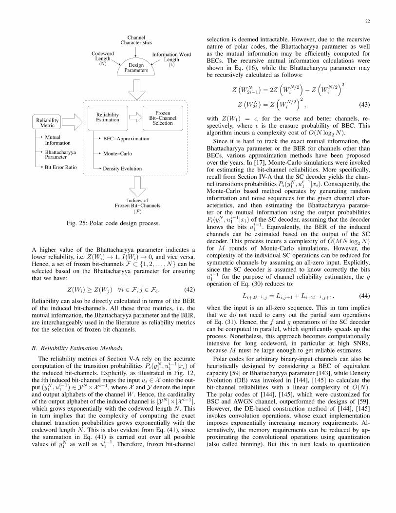
22

Bit−ChannelFrozen

Selection

DesignParameters

CodewordLength

Information WordLength

ChannelCharacteristics

EstimationReliability

BEC−Approximation

Monte−Carlo

Density Evolution

MetricReliability

Mutual

Bhattacharyya

Bit Error Ratio

Information

Parameter

Indices ofFrozen Bit−Channels

(N) (k)

(F)

Fig. 25: Polar code design process.

A higher value of the Bhattacharyya parameter indicates alower reliability, i.e. Z(Wi)→ 1, I(Wi)→ 0, and vice versa.Hence, a set of frozen bit-channels F ⊂ {1, 2, . . . , N} can beselected based on the Bhattacharyya parameter for ensuringthat we have:

Z(Wi) ≥ Z(Wj) ∀i ∈ F , j ∈ Fc. (42)

Reliability can also be directly calculated in terms of the BERof the induced bit-channels. All these three metrics, i.e. themutual information, the Bhattacharyya parameter and the BER,are interchangeably used in the literature as reliability metricsfor the selection of frozen bit-channels.

B. Reliability Estimation Methods

The reliability metrics of Section V-A rely on the accuratecomputation of the transition probabilities Pi(yN1 , u

i−11 |xi) of

the induced bit-channels. Explicitly, as illustrated in Fig. 12,the ith induced bit-channel maps the input ui ∈ X onto the out-put (yN1 , u

i−11 ) ∈ YN×X i−1, where X and Y denote the input

and output alphabets of the channel W . Hence, the cardinalityof the output alphabet of the induced channel is |YN |×|X i−1|,which grows exponentially with the codeword length N . Thisin turn implies that the complexity of computing the exactchannel transition probabilities grows exponentially with thecodeword length N . This is also evident from Eq. (41), sincethe summation in Eq. (41) is carried out over all possiblevalues of yN1 as well as ui−11 . Therefore, frozen bit-channel

selection is deemed intractable. However, due to the recursivenature of polar codes, the Bhattacharyya parameter as wellas the mutual information may be efficiently computed forBECs. The recursive mutual information calculations wereshown in Eq. (16), while the Bhattacharyya parameter maybe recursively calculated as follows:

Z(WN

2i−1)= 2Z

(W

N/2i

)− Z

(W

N/2i

)2

Z(WN

2i

)= Z

(W

N/2i

)2, (43)

with Z(W1) = ε, for the worse and better channels, re-spectively, where ε is the erasure probability of BEC. Thisalgorithm incurs a complexity cost of O(N log2N).

Since it is hard to track the exact mutual information, theBhattacharyya parameter or the BER for channels other thanBECs, various approximation methods have been proposedover the years. In [17], Monte-Carlo simulations were invokedfor estimating the bit-channel reliabilities. More specifically,recall from Section IV-A that the SC decoder yields the chan-nel transitions probabilities Pi(yN1 , u

i−11 |xi). Consequently, the

Monte-Carlo based method operates by generating randominformation and noise sequences for the given channel char-acteristics, and then estimating the Bhattacharyya parame-ter or the mutual information using the output probabilitiesPi(y

N1 , u

i−11 |xi) of the SC decoder, assuming that the decoder

knows the bits ui−11 . Equivalently, the BER of the inducedchannels can be estimated based on the output of the SCdecoder. This process incurs a complexity of O(MN log2N)for M rounds of Monte-Carlo simulations. However, thecomplexity of the individual SC operations can be reduced forsymmetric channels by assuming an all-zero input. Explicitly,since the SC decoder is assumed to know correctly the bitsui−11 for the purpose of channel reliability estimation, the goperation of Eq. (30) reduces to:

Li+2j−1,j = Li,j+1 + Li+2j−1,j+1. (44)

when the input is an all-zero sequence. This in turn impliesthat we do not need to carry out the partial sum operationsof Eq. (31). Hence, the f and g operations of the SC decodercan be computed in parallel, which significantly speeds up theprocess. Nonetheless, this approach becomes computationallyintensive for long codeword, in particular at high SNRs,because M must be large enough to get reliable estimates.

Polar codes for arbitrary binary-input channels can also beheuristically designed by considering a BEC of equivalentcapacity [59] or Bhattacharyya parameter [143], while DensityEvolution (DE) was invoked in [144], [145] to calculate thebit-channel reliabilities with a linear complexity of O(N).The polar codes of [144], [145], which were customized forBSC and AWGN channel, outperformed the designs of [59].However, the DE-based construction method of [144], [145]invokes convolution operations, whose exact implementationimposes exponentially increasing memory requirements. Al-ternatively, the memory requirements can be reduced by ap-proximating the convolutional operations using quantization(also called binning). But this in turn leads to quantization

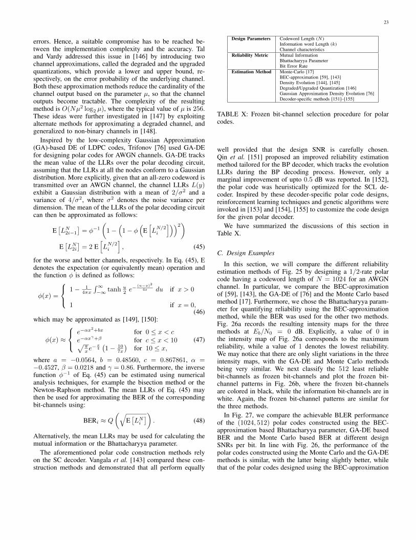
23

errors. Hence, a suitable compromise has to be reached be-tween the implementation complexity and the accuracy. Taland Vardy addressed this issue in [146] by introducing twochannel approximations, called the degraded and the upgradedquantizations, which provide a lower and upper bound, re-spectively, on the error probability of the underlying channel.Both these approximation methods reduce the cardinality of thechannel output based on the parameter µ, so that the channeloutputs become tractable. The complexity of the resultingmethod is O(Nµ2 log2 µ), where the typical value of µ is 256.These ideas were further investigated in [147] by exploitingalternate methods for approximating a degraded channel, andgeneralized to non-binary channels in [148].

Inspired by the low-complexity Gaussian Approximation(GA)-based DE of LDPC codes, Trifonov [76] used GA-DEfor designing polar codes for AWGN channels. GA-DE tracksthe mean value of the LLRs over the polar decoding circuit,assuming that the LLRs at all the nodes conform to a Gaussiandistribution. More explicitly, given that an all-zero codeword istransmitted over an AWGN channel, the channel LLRs L(y)exhibit a Gaussian distribution with a mean of 2/σ2 and avariance of 4/σ2, where σ2 denotes the noise variance perdimension. The mean of the LLRs of the polar decoding circuitcan then be approximated as follows:

E[LN2i−1

]= φ−1

(1−

(1− φ

(E[LN/2i

]))2)

E[LN2i]= 2 E

[LN/2i

], (45)

for the worse and better channels, respectively. In Eq. (45), Edenotes the expectation (or equivalently mean) operation andthe function φ is defined as follows:

φ(x) =

1− 14πx

∫∞−∞ tanh u

2 e− (u−x)2

4x du if x > 0

1 if x = 0,(46)

which may be approximated as [149], [150]:

φ(x) ≈

e−αx2+bx for 0 ≤ x < c

e−αxγ+β for c ≤ x < 10√

πxe− x4(1− 10

7x

)for 10 ≤ x,

(47)

where a = −0.0564, b = 0.48560, c = 0.867861, α =−0.4527, β = 0.0218 and γ = 0.86. Furthermore, the inversefunction φ−1 of Eq. (45) can be estimated using numericalanalysis techniques, for example the bisection method or theNewton-Raphson method. The mean LLRs of Eq. (45) maythen be used for approximating the BER of the correspondingbit-channels using:

BERi ≈ Q(√

E[LNi])

. (48)

Alternatively, the mean LLRs may be used for calculating themutual information or the Bhattacharyya parameter.

The aforementioned polar code construction methods relyon the SC decoder. Vangala et al. [143] compared these con-struction methods and demonstrated that all perform equally

Design Parameters Codeword Length (N )Information word Length (k)Channel characteristics

Reliability Metric Mutual InformationBhattacharyya ParameterBit Error Rate

Estimation Method Monte-Carlo [17]BEC-approximation [59], [143]Density Evolution [144], [145]Degraded/Upgraded Quantization [146]Gaussian Approximation Density Evolution [76]Decoder-specific methods [151]–[155]

TABLE X: Frozen bit-channel selection procedure for polarcodes.

well provided that the design SNR is carefully chosen.Qin et al. [151] proposed an improved reliability estimationmethod tailored for the BP decoder, which tracks the evolutionLLRs during the BP decoding process. However, only amarginal improvement of upto 0.5 dB was reported. In [152],the polar code was heuristically optimized for the SCL de-coder. Inspired by these decoder-specific polar code designs,reinforcement learning techniques and genetic algorithms wereinvoked in [153] and [154], [155] to customize the code designfor the given polar decoder.

We have summarized the discussions of this section inTable X.

C. Design Examples

In this section, we will compare the different reliabilityestimation methods of Fig. 25 by designing a 1/2-rate polarcode having a codeword length of N = 1024 for an AWGNchannel. In particular, we compare the BEC-approximationof [59], [143], the GA-DE of [76] and the Monte Carlo basedmethod [17]. Furthermore, we chose the Bhattacharyya param-eter for quantifying reliability using the BEC-approximationmethod, while the BER was used for the other two methods.Fig. 26a records the resulting intensity maps for the threemethods at Eb/N0 = 0 dB. Explicitly, a value of 0 inthe intensity map of Fig. 26a corresponds to the maximumreliability, while a value of 1 denotes the lowest reliability.We may notice that there are only slight variations in the threeintensity maps, with the GA-DE and Monte Carlo methodsbeing very similar. We next classify the 512 least reliablebit-channels as frozen bit-channels and plot the frozen bit-channel patterns in Fig. 26b, where the frozen bit-channelsare colored in black, while the information bit-channels are inwhite. Again, the frozen bit-channel patterns are similar forthe three methods.

In Fig. 27, we compare the achievable BLER performanceof the (1024, 512) polar codes constructed using the BEC-approximation based Bhattacharyya parameter, GA-DE basedBER and the Monte Carlo based BER at different designSNRs per bit. In line with Fig. 26, the performance of thepolar codes constructed using the Monte Carlo and the GA-DEmethods is similar, with the latter being slightly better, whilethat of the polar codes designed using the BEC-approximation

24

0

0.5

1

0

0.2

0.4

200 400 600 800 1000

Channel Index

0

0.2

0.4

BEC-Approximation

GA-DE

Monte Carlo

(a) Reliability intensity. Please note that a value of 0 implieshigh reliability, since the reliability metric is the Bhattacharyyaparameter for BEC-approximation and the BER for GA-DEand Monte Carlo.

200 400 600 800 1000

Channel Index

BEC-Approximation

GA-DE

Monte Carlo

(b) Frozen bit-channel patterns. The black regions denote thefrozen indices, while the white one is for information indices.

Fig. 26: Comparison of polar code construction methods atEbN0

= 0 dB: BEC-approximation based Bhattacharyya param-eter, GA-DE based BER and Monte Carlo based BER.

method is worse. Furthermore, Fig. 27 shows that the BLERperformance of the Monte Carlo and the GA-DE methods isonly sightly affected, when the design SNR per bit is increasedfrom 0 dB to 2 dB. It is obvious that if we choose a very lowor high value of the design SNR per bit, then the performancewill get worse, as demonstrated in [143]. Hence, the polarcode construction method is not very sensitive to reasonablediscrepancies between the design SNR and the operating SNR.We have also benchmarked the designed polar codes againstthe 3GPP 5G NR polar code in Fig. 27. It may be observedthat the performance of the Monte Carlo and the GA-DE basedpolar codes approaches that of the 3GPP 5G NR when thedesign Eb/N0 = 2 dB.

-1 0 1 2 3 4 5

Eb/N

0 [dB]

10-3

10-2

10-1

100

BLE

R

Bhattacharya 0 dB

Bhattacharya 1 dB

Bhattacharya 2 dB

BER-MC 0 dB

BER-MC 1 dB

BER-MC 2 dB

BER-GA 0 dB

BER-GA 1 dB

BER-GA 2 dB

3GPP sequence

Fig. 27: Comparison of the achievable BLER performance ofthe (1024, 512) polar codes constructed using the various reli-ability estimation methods of Section V-B at different designSNRs per bit. The performance is benchmarked against the3GPP 5G NR frozen bit-channel sequence. An SCL decoderhaving L = 8 and QPSK transmission over an AWGN channelwas used.

VI. QUANTUM-TO-CLASSICAL ISOMORPHISM

In contrast to a classical bit, which can be either 0 or 1 at anyparticular instant, a quantum bit (qubit)6 exists in superpositionof the orthogonal basis states |0〉 and |1〉. This superimposedstate of the qubit is generally described using the state vectoras follows:

|ψ〉 = α|0〉+ β|1〉, (49)

where |·〉 is called Ket or Dirac notation [157], and α and βare complex coefficients conforming to:

|α|2 + |β|2 = 1. (50)

Furthermore, unlike a classical bit, which can be ‘observed’ (or‘measured’) without disturbing its value, any observation of thequbit perturbs its superimposed state of Eq. (49). To elaborate,if a qubit is observed in the computational basis7, it maycollapse to the state |0〉 with a probability of |α|2 and the state|1〉 with a probability of |β|2. The quantum superposition ofEq. (49) makes quantum processing (or computation) systemsinherently parallel, while the observation property togetherwith the quantum no-cloning theorem8 makes quantum trans-missions absolutely secure. However, these unusual quantumcharacteristics, which have no counterpart in the classical

6Please refer to [156] for deeper insights into the duality of the classicaland the quantum regime.

7The pair of orthogonal basis states |0〉 and |1〉 is called the computationalbasis.

8According to the quantum no-cloning theorem, arbitrary quantum statescannot be cloned (or copied) [158].

25

domain, make it challenging to design Quantum Error Correc-tion Codes (QECCs). Nonetheless, there exists an underlyingisomorphism between the classical and quantum paradigms,which can be exploited for designing efficient QECCs fromthe known classical codes [156], [159], [160].

Environmental decoherence is a major source of noise inquantum systems. It can be modeled using a depolarizingchannel, which is considered the ‘worst-case scenario’ [161].Explicitly, a quantum depolarizing channel characterized bythe depolarizing probability p independently inflicts an error oneach qubit, such that a qubit may experience a bit-flip (Pauli-X), a phase-flip (Pauli-Z) or a bit-and-phase-flip (Pauli-Y)error with a probability of p/3 each9. Hence, in contrast tothe classical channels, which only inflict bit-flip errors, thequantum depolarizing channel imposes both bit-flip as well asphase-flip errors. An interesting point to notice here is that aquantum depolarizing channel may also be viewed as a pair ofcorrelated BSCs inflicting bit-flips and phase-flips respectively.Fortunately, classical polar codes are capable of concurrentlypolarizing both the bit-flip as well as the phase-flip channels,when the classical XOR gates are replaced by the quantumControlled NOT (CNOT) gates10; hence achieving the quantumchannel capacity, as demonstrated in [162], [163]. This isbecause polar codes merely rely on CNOT gates for channelpolarization, which are capable of concurrently polarizing boththe bit-flip as well as the phase-flip channels, but in oppositedirections, as further discussed below.

QECCs exploit the computational basis for correcting bit-flip errors, while the Hadamard basis11 is used for phase-flip correction. The action of CNOT on the Hadamard basisis analogous to that on the computational basis with therole of control and target qubits swapped. Explicitly, let usconsider the two-qubit state |+−〉 in Hadamard basis, whichis equivalent to:

|+−〉 = 1√2(|0〉+ |1〉)⊗ 1√

2(|0〉 − |1〉)

=1

2(|00〉 − |01〉+ |10〉 − |11〉) , (51)

in the computational basis. When a CNOT gate is applied to

9The I, X, Y and Z are single-qubit Pauli operators (or gates) defined as:

I =

(1 00 1

), X =

(0 11 0

), Z =

(1 00 −1

), Y =

(0 −ii 0

).

10The CNOT gate is a two-qubit gate, having a control qubit and a targetqubit. When the control qubit is in state |1〉, the target qubit is flipped;otherwise, the target qubit is left unchanged, as encapsulated below:

CNOT (|ψ0〉, |ψ1〉) = |ψ0〉 ⊗ |ψ0 ⊕ ψ1〉,

where |ψ0〉 is the control qubit, while |ψ1〉 is the target qubit. Hence, CNOTgate is the quantum analogue of the classical XOR gate.

11The pair of orthogonal basis states |+〉 and |−〉 is called the Hadamardbasis, where the basis states |+〉 and |−〉 are defined as:

|+〉 4= 1√2(|0〉+ |1〉) , |−〉 4= 1√

2(|0〉 − |1〉) .

H H

≡

Z

Fig. 28: A CNOT gate is equivalent to a Controlled-Z(Cz) gate, with the control and target qubits swapped, whenHadamard gates are invoked at the input and output. The circuitto the left flips the top qubit in computational basis (|0〉 and|1〉), when the bottom qubit is in the state |1〉, while the circuitto the right flips the botton qubit in the Hadamard basis (|+〉and |−〉), when the top qubit is in the state |−〉.

|u1 ⊕ u2〉

|u2〉

W1 = W−B

W2 = W+B

W

W

|u1〉

|u2〉

(a) Polarization in the computa-tional basis, resulting in polarizedbit-flip channels.

W1 = W+P

W2 = W−P

|u1〉H H

Z W

W

ZH|u1〉|u2〉

|u1〉

|u2〉

(b) Polarization in the Hadamardbasis, resulting in polarized phase-flip channels.

Fig. 29: The 2-qubit kernel of a quantum polar code in thecomputational and Hadamard bases.

the second qubit controlled by the first qubit, we get:

|+−〉 CNOT(1, 2)−−−−−−−−→1

2(|00〉 − |01〉+ |11〉 − |10〉) = | − −〉.

(52)

We may observe in Eq. (52) that the operation of CNOT(1, 2)on the computational basis is equivalent to that of CNOT(2, 1)on the Hadamard basis. More explicitly, the classic CNOT(i, j)acting on the computational basis flips the jth qubit (target)between |0〉 and |1〉, when the ith qubit (control) is in the state|1〉. This operation is analogous to that of CNOT(j, i) acting onthe Hadamard basis, which flips the ith qubit (target) between|+〉 and |−〉, when the jth qubit (control) is in the state |−〉.More specifically, a CNOT gate may also be implementedusing a Controlled-Z (Cz) gate, with the control and targetqubits swapped, as shown in Fig. 28.

Let us now consider the 2-qubit kernel of polar code given inFig. 29a, which is the quantum-domain equivalent of Arikan’skernel of Fig. 5a. From the perspective of the computationalbasis, the encoder of Fig. 29a combines the information ofthe two channels in the computational basis, so that thecomputational basis information of the |u2〉 is redundantlyadded to that of |u1〉 (⊕ denotes modulo-2 addition in the

26

computational basis). Consequently, the second qubit-channelW2 becomes more robust against bit-flip errors at the costof deteriorating the robustness of the first qubit-channel W1.In other words, W2 tends to polarize towards a better bit-flip channel W+

B , while W1 tends to polarize towards a worsebit-flip channel W−B . However, the total capacity of the twochannels is conserved.

Fig. 29b shows the polar encoder from the perspective ofthe Hadamard basis; hence, the CNOT gate is replaced by theequivalent circuit of Fig. 28, which invokes the Cz gate. Moreexplicitly, in Fig. 29b, the Hadamard basis information of thefirst qubit |u1〉 is redundantly incorporated in the Hadamardbasis information of the second qubit. Consequently, the in-formation carrying capacity of the first qubit-channel W1 isenhanced in the phase basis, while that of the second qubit-channel W2 degrades in the phase basis. Hence, the firstqubit-channel W1 tends to polarize towards a better phase-flipchannel, while the second qubit-channel W2 tends to polarizetowards a worse phase-flip channel, denoted by W+

P and W−P ,respectively. Therefore, the elementary kernal of a polar codeis capable of polarizing both the bit-flip as well as phase-flip channels, but the direction of polarization is opposite, asillustrated in Fig. 29.

Based on the above discussions, a quantum polar codeinduces four sets of channels, covering both the bit-flip aswell as the phase-flip errors. Explicitly, the polarized channelsmay belong to one of the following four sets:

1) Good bit-and-phase channels (Fc): These inducedchannels exhibit high information carrying capacity inthe computational basis (bit-flip) as well as in theHadamard basis (phase-flip). Consequently, these in-duced channels are used for transmitting the uncodedqubits.

2) Good bit-only channels (FP ): These channels havehigh information carrying capacity in the computationalbasis (bit-flip), but low capacity in the Hadamard basis(phase-flip). Hence, these channels are frozen in theHadamard basis by transmitting the Hadamard basisstates |+〉 or |−〉, which are known to the receiver.

3) Good phase-only channels (FB): These channels havelow information carrying capacity in the computationalbasis (bit-flip), but high capacity in the Hadamard basis(phase-flip). Consequently, they are frozen in the com-putational basis, hence transmitting the computationalbasis states |0〉 or |1〉, which are known to the receiver.

4) Bad bit-and-phase channels (FBP ): These channelshave low information carrying capacity in both the com-putational basis (bit-flip) as well as the Hadamard basis(phase-flip). Consequently, these channels are frozen inboth the computational as well as the Hadamard bases.

This is achieved by exploiting pre-shared entangled12

qubits, which are referred to as ebits. Explicitly, ebitsare created in the Bell state |φ+〉, expressed as:

|φ+〉 = |00〉TXRX + |11〉TXRX√

2, (53)

so that the first qubit is retained at the transmitter(TX ), while the associated entangled qubit is sent to thereceiver (RX ) before actual transmission commences,for example during off-peak hours, when the chan-nels are under-utilized. It is generally assumed thatthe pre-sharing of ebits takes place over a noiselessquantum channel. Hence, quantum polar codes intrin-sically belong to the family of entanglement-assistedQECCs [165], [166].

VII. QUANTUM POLAR CODES

Inspired by the provably capacity achieving nature of classi-cal polar codes as well as their efficient encoding and decodingstructures, Wilde and Guha [167] were the first to demonstratethe existence of the channel polarization phenomenon forclassical-quantum channels, which transmit classical informa-tion over quantum channels. These ideas were later extendedto the transmission of quantum information in [162]. Thequantum polar codes of [162], [167] exploit the same encoderas Arikan’s polar codes, except that the classical XOR gatesare replaced by the quantum CNOT gates. Consequently, thequantum polar encoders of [162], [167] inherently benefitfrom the low encoding complexity of Arikan’s classic polarcodes. Furthermore, a quantum counterpart of the classicalSC decoder, named Quantum Successive Cancellation Decoder(QSCD), was conceived in [162], [167], which makes collec-tive measurement on all channel uses. This is achieved by ex-ploiting quantum hypothesis testing [168], [169] in conjunctionwith Sen’s noncommutative union bound [170]. The QSCDof [162], [167] failed to match the low decoding complexityof the classical SC decoder. This issue was addressed byRenes et al. in [171], where an efficient implementation ofa quantum polar decoder was given for quantum Pauli13

and erasure channels. Finally, Wilde and Renes combinedtheir efforts in [163], [172] to present an efficient QSCD forarbitrary quantum channels. The quantum polar codes of [162],[167], [171] rely on the sharing of noiseless ebits between thetransmitter and the receiver. In this context, the first unassistedquantum polar codes, consisting of concatenated bit-flip (com-putational basis) and phase-flip (Hadamard basis) correction

12‘Entanglement’, which Einstein termed as a ‘spooky action at a dis-tance’ [164], is the mysterious, correlation-like property between two or morequbits, which implies that the entangled qubits cannot be expressed as thetensor product of the individual qubits. Furthermore, a strange relationshipexists between the two entangled qubits, which entails that measuring oneof them also reveals the value of the other, even if they are geographicallyseparated.

13A quantum Pauli channel independently inflicts an error on each qubit,such that a qubit may experience a bit-flip (Pauli-X), a phase-flip (Pauli-Z)and a bit-and-phase-flip (Pauli-Y) error with a probability of px, pz and py ,respectively. A Quantum depolarizing channel is a special case of a Paulichannel having px = pz = py = p/3.

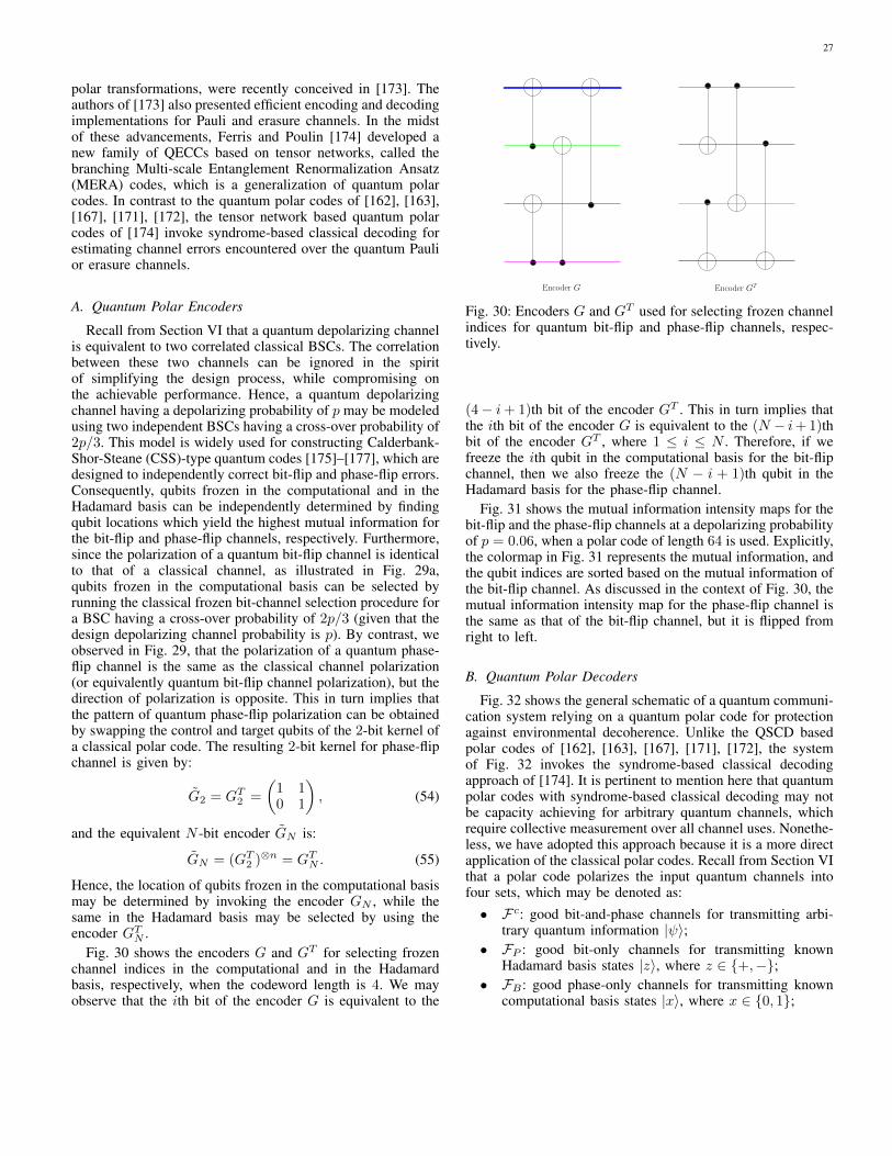
27

polar transformations, were recently conceived in [173]. Theauthors of [173] also presented efficient encoding and decodingimplementations for Pauli and erasure channels. In the midstof these advancements, Ferris and Poulin [174] developed anew family of QECCs based on tensor networks, called thebranching Multi-scale Entanglement Renormalization Ansatz(MERA) codes, which is a generalization of quantum polarcodes. In contrast to the quantum polar codes of [162], [163],[167], [171], [172], the tensor network based quantum polarcodes of [174] invoke syndrome-based classical decoding forestimating channel errors encountered over the quantum Paulior erasure channels.

A. Quantum Polar Encoders

Recall from Section VI that a quantum depolarizing channelis equivalent to two correlated classical BSCs. The correlationbetween these two channels can be ignored in the spiritof simplifying the design process, while compromising onthe achievable performance. Hence, a quantum depolarizingchannel having a depolarizing probability of p may be modeledusing two independent BSCs having a cross-over probability of2p/3. This model is widely used for constructing Calderbank-Shor-Steane (CSS)-type quantum codes [175]–[177], which aredesigned to independently correct bit-flip and phase-flip errors.Consequently, qubits frozen in the computational and in theHadamard basis can be independently determined by findingqubit locations which yield the highest mutual information forthe bit-flip and phase-flip channels, respectively. Furthermore,since the polarization of a quantum bit-flip channel is identicalto that of a classical channel, as illustrated in Fig. 29a,qubits frozen in the computational basis can be selected byrunning the classical frozen bit-channel selection procedure fora BSC having a cross-over probability of 2p/3 (given that thedesign depolarizing channel probability is p). By contrast, weobserved in Fig. 29, that the polarization of a quantum phase-flip channel is the same as the classical channel polarization(or equivalently quantum bit-flip channel polarization), but thedirection of polarization is opposite. This in turn implies thatthe pattern of quantum phase-flip polarization can be obtainedby swapping the control and target qubits of the 2-bit kernel ofa classical polar code. The resulting 2-bit kernel for phase-flipchannel is given by:

G2 = GT2 =

(1 10 1

), (54)

and the equivalent N -bit encoder GN is:

GN = (GT2 )⊗n = GTN . (55)

Hence, the location of qubits frozen in the computational basismay be determined by invoking the encoder GN , while thesame in the Hadamard basis may be selected by using theencoder GTN .

Fig. 30 shows the encoders G and GT for selecting frozenchannel indices in the computational and in the Hadamardbasis, respectively, when the codeword length is 4. We mayobserve that the ith bit of the encoder G is equivalent to the

Encoder G Encoder GT

Fig. 30: Encoders G and GT used for selecting frozen channelindices for quantum bit-flip and phase-flip channels, respec-tively.

(4− i+ 1)th bit of the encoder GT . This in turn implies thatthe ith bit of the encoder G is equivalent to the (N − i+1)thbit of the encoder GT , where 1 ≤ i ≤ N . Therefore, if wefreeze the ith qubit in the computational basis for the bit-flipchannel, then we also freeze the (N − i + 1)th qubit in theHadamard basis for the phase-flip channel.

Fig. 31 shows the mutual information intensity maps for thebit-flip and the phase-flip channels at a depolarizing probabilityof p = 0.06, when a polar code of length 64 is used. Explicitly,the colormap in Fig. 31 represents the mutual information, andthe qubit indices are sorted based on the mutual information ofthe bit-flip channel. As discussed in the context of Fig. 30, themutual information intensity map for the phase-flip channel isthe same as that of the bit-flip channel, but it is flipped fromright to left.

B. Quantum Polar Decoders

Fig. 32 shows the general schematic of a quantum communi-cation system relying on a quantum polar code for protectionagainst environmental decoherence. Unlike the QSCD basedpolar codes of [162], [163], [167], [171], [172], the systemof Fig. 32 invokes the syndrome-based classical decodingapproach of [174]. It is pertinent to mention here that quantumpolar codes with syndrome-based classical decoding may notbe capacity achieving for arbitrary quantum channels, whichrequire collective measurement over all channel uses. Nonethe-less, we have adopted this approach because it is a more directapplication of the classical polar codes. Recall from Section VIthat a polar code polarizes the input quantum channels intofour sets, which may be denoted as:• Fc: good bit-and-phase channels for transmitting arbi-

trary quantum information |ψ〉;• FP : good bit-only channels for transmitting known

Hadamard basis states |z〉, where z ∈ {+,−};• FB : good phase-only channels for transmitting known

computational basis states |x〉, where x ∈ {0, 1};

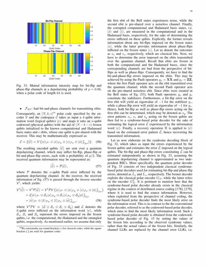
28

Bit-Flip Channel

10 20 30 40 50 60

Qubit Index

0.2

0.4

0.6

0.8

1

Phase-Flip Channel

10 20 30 40 50 60

Qubit Index

0.2

0.4

0.6

0.8

1

Fig. 31: Mutual information intensity map for bit-flip andphase-flip channels at a depolarizing probability of p = 0.06,when a polar code of length 64 is used.

• FBP : bad bit-and-phase channels for transmitting ebits.

Consequently, an [N, k, c]14 polar code specified by the en-coder V and the codespace C takes as input a k-qubit infor-mation word (logical qubits) |ψ〉 and maps it onto an n-qubitcodeword (physical qubits) with the aid of (N −k− c) frozenqubits initialized to the known computational and Hadamardbasis states and c ebits, whose one qubit is pre-shared with thereceiver. This may be mathematically expressed as:

C = {|ψ〉 = V(|ψ〉Fc ⊗ |x〉FB ⊗ |z〉FP ⊗ |φ〉+FBP

)}. (56)

The resulting encoded qubits |ψ〉 are sent over a quantumdepolarizing channel, which may inflict bit-flip, phase-flip orbit-and-phase-flip errors, each with a probability of p/3. Thereceived quantum information may be represented as:

|ψ〉 = P|ψ〉, (57)

where P denotes the n-qubit Pauli error inflicted by thequantum depolarizing channel. At the receiver, the receivedinformation of Eq. (57) is passed through the inverse encoderV†, which yields:

V†|ψ〉 = V†P|ψ〉 = V†PV(|ψ〉Fc ⊗ |x〉FB ⊗ |z〉FP ⊗ |φ〉+FBP

)

= L|ψ〉Fc ⊗ Sx|x〉FB ⊗ Sz|z〉FP ⊗ Sy|φ〉+FBP= |ψ〉Fc ⊗ |x〉FB ⊗ |z〉FP ⊗ |φ〉+FBP . (58)

where V†PV ≡ (L ⊗ Sx ⊗ Sz ⊗ Sy) and L denotes thek-qubit error inflicted on the information word |ψ〉, whileSx, Sz and Sy represent the errors imposed on the frozenqubits, i.e. the computational, the Hadamard and the entangledqubits, respectively. As mentioned earlier, we assume that only

14We consistently use round brackets (.) for classical codes, while the squarebrackets [.] are used for quantum codes.

the first ebit of the Bell states experiences noise, while thesecond ebit is pre-shared over a noiseless channel. Finally,the corrupted computational and Hadamard basis states, i.e.|x〉 and |z〉, are measured in the computational and in theHadamard basis, respectively, for the sake of determining theerrors inflicted on these qubits. Explicitly, the former revealsinformation about any bit-flips imposed on the frozen states|x〉, while the latter provides information about phase-flipsinflicted on the frozen states |z〉. Let us denote the outcomesas sx and sz , respectively, which are classical bits. Next, wehave to determine the error imposed on the ebits transmittedover the quantum channel. Recall that ebits are frozen inboth the computational and the Hadamard bases, since thecorresponding channels are bad from the perspective of bit-flips as well as phase-flips. Consequently, we have to find thebit-and-phase-flip errors imposed on the ebits. This may beachieved by using the Pauli operators gx = XX and gz = ZZ,where the first Pauli operator acts on the ebit transmitted overthe quantum channel, while the second Pauli operator actson the pre-shared noiseless ebit. Since ebits were created inthe Bell states of Eq. (53), both Pauli operators gx and gzconstitute the stabilizers. Furthermore, a bit-flip error on thefirst ebit will yield an eigenvalue of −1 for the stabilizer gz ,while a phase-flip error will yield an eigenvalue of −1 for gx.Hence, both bit-flip as well as phase-flip errors acting on thefirst ebit can be determined, which may be denoted as sy . Theerror patterns sx, sz and sy acting on the frozen qubits arethen fed to a syndrome-based polar decoder for the sake ofestimating the logical error L experienced by the informationword |ψ〉. Finally, a recovery operation R is applied to |ψ〉based on the estimated error pattern L, hence recovering thetransmitted information.

Let us now elaborate on the syndrome decoding block ofFig. 32, which takes as input the errors experienced by thefrozen qubits and estimates the error L imposed on the logicalqubits. The bit-flip and phase-flip errors constituting L can beestimated independently as shown in Fig. 33, assuming thequantum depolarizing channel is approximated as two inde-pendent BSCs. More specifically, the quantum polar decoderof Fig. 33 consists of two independent classical syndrome-based polar decoders used for estimating bit-flip and phase-fliperrors, denoted as Lx and Lz , respectively. The former decoderexploits the classical polar encoder GN , while the latter relieson the encoder GTN . It is pertinent to mention here that thesyndrome-based polar decoder already exists in the classicalregime in the context of distributed source coding [178], [179],where it is used to find the source information. However,when exploited from the perspective of channel coding, thesyndrome-based polar decoder finds the most likely error onthe information word. This is in contrast to the the conventionalpolar decoder, referred to as the codeword-based polar decoder,which aims to find the most likely information word. Such asyndrome-based polar decoder is obtained from the codeword-based polar decoder of Fig. 15 by setting the values ofthe frozen bits according to the observed syndrome values,rather than the actual values of the frozen bits. Similarly, thechannel LLRs are replaced by the channel error LLRs, i.e.

29

SyndromeDecoding

R

TXgxgz

|ψ〉|x〉FB

|ψ〉Fc

L|ψ〉Fc

|ψ〉Fc

RX

Mz

|z〉FP

|φ+〉FBP

Quantum Channel|ψ〉

|z〉FP

V

|φ+〉FBP

(sz)FP

(sy)FBP

V†Mx

(sx)FB|x〉FB

Fig. 32: Schematic of a quantum communication system relying on a syndrome decoding based quantum polar code.

ClassicalSyndome−basedPolar Decoder

ClassicalSyndome−basedPolar Decoder Binary

To

Pauli

Mapping

(GTN)

(GN)

Lx

Lz

L

(sx)FB

(sz)FP

(sy)FBP

Fig. 33: Schematic of quantum polar decoder.

(Lz, Lx) L Estimated Error(0, 0) I No Error(0, 1) X Bit-flip Error(1, 0) Z Phase-flip Error(1, 1) Y Bit-and-phase-flip Error

TABLE XI: Binary to Pauli mapping for estimating the Paulierror.

the probability of encountering channel error on the codedsequence. In case of a depolarizing channel, or equivalentlya BSC channel, the channel error LLRs are set according tothe marginalized depolarizing probability 2p/3. The rest ofthe decoding process is the same as that of the codeword-based decoding. Finally, the estimated error patterns Lx andLz are mapped onto the corresponding Pauli operators usingthe binary-to-Pauli mapping of Table XI, hence yielding thePauli error L.

VIII. CONCLUSIONS & FUTURE DIRECTIONS

To conclude, Arikan’s polarization phenomenon of Sec-tion II has paved the way to provably approach the Shannon’scapacity at low encoding and decoding complexity. In partic-ular, polar codes have structured encoders and decoders, as

discussed in Section III and Section IV, respectively, hencedispelling the notion that randomized coding structures aremore apt for approaching Shannon’s capacity. Furthermore,polar codes intrinsically support rate-adaptation, since thecoding rate can be varied by only changing the number offrozen bits, while retaining the same encoder and decoder.

The attractive features of polar codes have stimulated a waveof interest in the research community as well as in the industry.Consequently, within a decade of their inception, polar codeshave replaced their classic counterparts in the 5G NR for thecontrol channels of the eMBB use-case. However, the highdecoding latency of polar codes is a major concern restrictingthe widespread application of polar codes, as discussed in Sec-tion IV, where we have reviewed the major polar decoders withslow-paced tutorial examples. More specifically, recall fromTable IX that the different polar decoding schemes, namelythe SC of Section IV-A, the SSC of Section IV-B, the SCL ofSection IV-C, the SCS of Section IV-D, the BP of Section IV-Eand the SCAN of Section IV-F, entail a compromise betweenthe imposed complexity, space requirements, performance andthe tendency for fully-parallel implementation.

Another concern related to polar codes is their channel-specific nature, which necessitates the optimization of polarcodes for the channel under consideration. Explicitly, theoptimization of polar codes entails selecting the right indicesfor the frozen bit-channels. In Section V, we detail the polarcode design principles with particular emphasis on the BEC-approximation, Monte-Carlo and GA-DE methods for esti-mating the reliabilities of the bit-channels. Furthermore, weconstruct frozen bit-channel sequences for the AWGN channelusing these three methods and compare their performance. It isdemonstrated that the sequences constructed using the Monte-Carlo and GA-DE are equally good, while those designedusing the BEC-approximation have inferior performance. Wesurmise that, this is because a BEC does not accurately modeltransmission over an AWGN channel. We further demonstratethat, while the SNR is an important design parameter, limitedvariations in the design SNR only slightly affect the BLERperformance.

Polar codes have also been warmly welcomed by the quan-

30

tum coding community, since the notion of channel polariza-tion readily extends to the quantum channels. Interestingly,Arikan’s polar encoder is capable of concurrently polarizingthe bit-flip and phase-flip quantum channels, when the XORgates are replaced by quantum CNOT gates, as exemplifiedin Section VI. However, the QSCD is not a direct extensionof the classical SC decoder. The relevant contributions in thiscontext are briefly summarized in Section VII. Nonetheless,there exist quantum polar codes designed for quantum Paulichannels, which are more directly linked to the classical polarcodes, since they invoke the classical syndrome based polardecoders. The encoder and decoder of this class of quantumpolar codes are reviewed in Section VII-A and Section VII-B,respectively.

As surveyed in this paper, intensive research efforts havebeen invested in the polar coding paradigm over the last decadefor the sake of bringing it on par with its contemporaries,namely the turbo and LDPC codes. Nonetheless, there is agreat potential to explore this coding paradigm further, sinceit is still in its infancy. Some of the potential research directionsare discussed below:

1) Non-Arikan Polar Codes: As discussed in Sec-tion II-B, efforts have been made to design multi-dimensional as well as non-binary kernels for polarcodes. However, these kernels have not been able toreplace the Arikan’s kernel, owing to the associatedencoding and decoding complexities. This is still anopen research area. In particular, the non-binary kernelsare important from the perspective of source coding.

2) Low-Latency, Power-Resource-Efficient & FlexiblePolar Decoders: Polar decoder continues to be a majorconcern; hence preventing the adoption of polar codesfor the data channel of 5G NR. These include a rangeof open research problems both from the algorithmicperspective as well as from the implementation. Inparticular, the existing polar decoders incur a highlatency, which is a primary concern for URLLC appli-cations. Recall from Table IX that only the BP decodersupports fully-parallel implementation. However, this isachieved at cost both in terms of the performance, andits complexity as well as space requirement. substantialefforts have been made to partially parallelize the otherpolar decoders, for example in [79], [81], [82], [93],[121], but their latency still remains higher than thatof the turbo and LDPC codes, which lend themselvesto a convenient fully-parallel implementation [180]–[182]. Furthermore, there is a need to explore morepractical polar decoders as well as to develop furtherthe hardware implementations of the existing polardecoders to bring them at par with the turbo and LDPCcodes, particularly from the perspective of latency (orthroughput), power efficiency, resource efficiency aswell as flexibility. From the algorithmic perspective,soft-in soft-out polar decoding is also a promisingresearch avenue, since the existing soft SCL decoderis only applicable to systematic polar codes, while theperformance of the SCAN decoder is not at par with

that of the SCL decoder. So, a more general soft SCLdecoder is required for concatenated frameworks, forexample concatenated coding schemes or joint detectionand decoding schemes, invoking iterative decoding.

3) Stochastic Polar Decoders: Stochastic LDPC andturbo decoders are known to provide attractive benefitsboth in terms of fault-tolerance (to timing errors) aswell as latency (or throughput) [183], [184]. However,stochastic polar decoders have not attracted much at-tention, apart from the contributions in [185]–[190].Since the latency of polar decoders is already a primeconcern, in this context it is worth investigating the areaof stochastic polar decoders.

4) Universal Polar Codes: Perhaps another limitationof polar codes is their channel-specific nature, whichnecessitates code optimization for the required channelcharacteristics. The impact of this is not very signifi-cant in practical scenarios. Hence, despite the channel-specific nature of polar codes, they have been adoptedfor the control channels of the 5G NR. However, thisstill remains a concern, especially from the theoreticalperspective. More specifically, polar codes with SCdecoding incur a capacity loss over compound chan-nels15, as demonstrated in [191]. This capacity lossis due to the sub-optimal SC decoding and may bealleviated by invoking the optimal ML decoding, astheoretically shown in [35]. Explicitly, it was demon-strated in [35] that a polar code optimized for a BSCis universal under ML decoding and hence is optimalfor any channel of equivalent capacity. Unfortunately,ML decoding of polar codes is not feasible. For thesake of overcoming this issue, universal polar codeswere conceived in [192], [193], which essentially retainthe low encoding and decoding complexity (per bit)of classic polar codes. However, this universality isachieved by increasing the length of polar codes, whichin turn imply a higher overall complexity and longerlatencies (or equivalently lower throughputs). This is apromising research avenue and must be explored furtherto find improved approaches for achieving universalityfor binary and non-binary classical polar codes as wellas for quantum polar codes.

REFERENCES

[1] C. Shannon, “A mathematical theory of communication, bell systemtechnical journal 27: 379-423 and 623–656,” Mathematical Reviews(MathSciNet): MR10, 133e, 1948.

[2] R. W. Hamming, “Error detecting and error correcting codes,” BellLabs Technical Journal, vol. 29, no. 2, pp. 147–160, 1950.

[3] I. Reed, “A class of multiple-error-correcting codes and the decodingscheme,” Transactions of the IRE Professional Group on InformationTheory, vol. 4, no. 4, pp. 38–49, September 1954.

[4] D. E. Muller, “Application of boolean algebra to switching circuitdesign and to error detection,” Transactions of the IRE ProfessionalGroup on Electronic Computers, no. 3, pp. 6–12, 1954.

15Compound channels model the transmission scenario where the exactchannel is unknown and only a set of channels to which the actual channelbelongs is known.

31

[5] A. Hocquenghem, “Codes Correcteurs d’Erreurs,” Chiffres (Paris),vol. 2, pp. 147–156, Sept. 1959.

[6] R. C. Bose and D. K. Ray-Chaudhuri, “On a class of error correctingbinary group codes,” Information and control, vol. 3, no. 1, pp. 68–79,1960.

[7] I. S. Reed and G. Solomon, “Polynomial codes over certain finitefields,” Journal of the society for industrial and applied mathematics,vol. 8, no. 2, pp. 300–304, 1960.

[8] R. W. Watson and C. W. Hastings, “Self-checked computation usingresidue arithmetic,” Proceedings of the IEEE, vol. 54, no. 12, pp.1920–1931, 1966.

[9] N. S. Szabo and R. I. Tanaka, Residue arithmetic and its applicationsto computer technology. McGraw-Hill, 1967.

[10] Blue Book: Recommendations for Space Data System Standards:Telemetry Channel Coding. Consultative Committee for Space DataSystems, May 1984.

[11] P. Elias, “Coding for noisy channels,” in IRE International ConventionRecord, 1955, pp. 37–46.

[12] R. Gallager, “Low-density parity-check codes,” IRE Transactions onInformation Theory, vol. 8, no. 1, pp. 21–28, January 1962.

[13] D. MacKay and R. M. Neal, “Good codes based on very sparsematrices,” Cryptography and Coding, pp. 100–111, 1995.

[14] D. J. MacKay and R. M. Neal, “Near Shannon limit performance oflow density parity check codes,” Electronics letters, vol. 32, no. 18,p. 1645, 1996.

[15] C. Berrou, A. Glavieux, and P. Thitimajshima, “Near Shannon limiterror-correcting coding and decoding: Turbo-codes. 1,” in TechnicalProgram of the IEEE International Conference on Communications,ICC ’93 Geneva, vol. 2, May 1993, pp. 1064–1070 vol.2.

[16] C. Berrou and A. Glavieux, “Near optimum error correcting codingand decoding: Turbo-codes,” IEEE Transactions on communications,vol. 44, no. 10, pp. 1261–1271, 1996.

[17] E. Arikan, “Channel polarization: A method for constructing capacity-achieving codes for symmetric binary-input memoryless channels,”IEEE Transactions on Information Theory, vol. 55, no. 7, pp. 3051–3073, July 2009.

[18] J. Hagenauer, E. Offer, and L. Papke, “Iterative decoding of binaryblock and convolutional codes,” IEEE Transactions on informationtheory, vol. 42, no. 2, pp. 429–445, 1996.

[19] H. Nickl, J. Hagenauer, and F. Burkert, “Approaching Shannon’scapacity limit by 0.2 dB using simple Hamming codes,” IEEE Com-munications Letters, vol. 1, no. 5, pp. 130–132, 1997.

[20] D. Divsalar, S. Dolinar and F. Pollara, “Serial concatenated trelliscoded modulation with rate-1 inner code,” in Proc. IEEE GlobalTelecommun. Conf., San Francisco, CA, Nov 2000, pp. 777–782.

[21] M. Tuchler and J. Hagenauer, “EXIT charts of irregular codes,”in Proceedings of Conference on Information Science and Systems,Princeton University, 20-22 March 2002, pp. 748–753.

[22] G. Ungerboeck, “Channel coding with multilevel/phase signals,” IEEETransactions on Information Theory, vol. 28, no. 1, pp. 55 – 67, Jan.1982.

[23] ——, “Trellis-coded modulation with redundant signal sets part I:Introduction,” IEEE Communications Magazine, vol. 25, no. 2, pp.5–11, February 1987.

[24] ——, “Trellis-coded modulation with redundant signal sets part II:State of the art,” IEEE Communications Magazine, vol. 25, no. 2, pp.12–21, February 1987.

[25] E. Zevahi, “8-PSK trellis codes for a Rayleigh fading channel,” IEEETransactions on Communications, vol. 40, pp. 873–883, 1992.

[26] G. Caire, G. Taricco, and E. Biglieri, “Bit-interleaved coded modu-lation,” IEEE transactions on information theory, vol. 44, no. 3, pp.927–946, 1998.

[27] X. Li and J. A. Ritcey, “Bit-interleaved coded modulation with iterative

decoding,” IEEE Communications Letters, vol. 1, no. 6, pp. 169–171,1997.

[28] P. Robertson and T. Worz, “Bandwidth-efficient turbo trellis-codedmodulation using punctured component codes,” IEEE Journal onSelected Areas in Communications, vol. 16, no. 2, pp. 206 – 218,Feb. 1998.

[29] V. Bioglio, C. Condo, and I. Land, “Design of polar codes in 5g newradio,” arXiv preprint arXiv:1804.04389, 2018.

[30] Z. B. K. Egilmez, L. Xiang, R. G. Maunder, and L. Hanzo, “Thedevelopment, design and performance of the 5G polar code,” IEEECommunications Surveys & Tutorials (submitted).

[31] K. Niu, K. Chen, J. Lin, and Q. T. Zhang, “Polar codes: Primaryconcepts and practical decoding algorithms,” IEEE CommunicationsMagazine, vol. 52, no. 7, pp. 192–203, July 2014.

[32] S. Shao, P. Hailes, T. Wang, J. Wu, R. G. Maunder, B. M. Al-Hashimi,and L. Hanzo, “Survey of turbo, LDPC and polar decoder ASICimplementations,” IEEE Communications Surveys Tutorials, pp. 1–1,2019.

[33] A. Wyner, “A definition of conditional mutual informationfor arbitrary ensembles,” Information and Control, vol. 38,no. 1, pp. 51 – 59, 1978. [Online]. Available:http://www.sciencedirect.com/science/article/pii/S0019995878900268

[34] E. Arikan, “A short course on polar coding (theory and applications),”Lecture Notes, Center for Wireless Communications, University ofOulu, May 2016.

[35] E. Sasoglu, “Polar coding theorems for discrete systems,” 2011.

[36] S. B. Korada, E. Sasoglu, and R. Urbanke, “Polar codes: Characteri-zation of exponent, bounds, and constructions,” IEEE Transactions onInformation Theory, vol. 56, no. 12, pp. 6253–6264, 2010.

[37] N. Presman, O. Shapira, and S. Litsyn, “Binary polar code kernelsfrom code decompositions,” in 2011 IEEE International Symposiumon Information Theory Proceedings, July 2011, pp. 179–183.

[38] N. Presman, O. Shapira, S. Litsyn, T. Etzion, and A. Vardy, “Binarypolarization kernels from code decompositions,” IEEE Transactionson Information Theory, vol. 61, no. 5, pp. 2227–2239, May 2015.

[39] P. Trifonov and V. Miloslavskaya, “Twisted polar codes,” in Interna-tional Symposium on Information Theory and its Applications, Oct2014, pp. 443–447.

[40] ——, “Polar codes with dynamic frozen symbols and their decodingby directed search,” in IEEE Information Theory Workshop (ITW),Sept 2013, pp. 1–5.

[41] ——, “Polar subcodes,” IEEE Journal on Selected Areas in Commu-nications, vol. 34, no. 2, pp. 254–266, Feb 2016.

[42] V. Bioglio and I. Land, “Polar-code construction of golay codes,” IEEECommunications Letters, vol. 22, no. 3, pp. 466–469, March 2018.

[43] E. Sasoglu, E. Telatar, and E. Arikan, “Polarization for arbitrarydiscrete memoryless channels,” in IEEE Information Theory Workshop,2009, pp. 144–148.

[44] E. Sasoglu, “Polar codes for discrete alphabets,” in IEEE InternationalSymposium on Information Theory Proceedings, July 2012, pp. 2137–2141.

[45] R. Mori and T. Tanaka, “Channel polarization on q-ary discretememoryless channels by arbitrary kernels,” in IEEE InternationalSymposium on Information Theory, June 2010, pp. 894–898.

[46] ——, “Non-binary polar codes using reed-solomon codes and alge-braic geometry codes,” in IEEE Information Theory Workshop (ITW),2010, pp. 1–5.

[47] ——, “Source and channel polarization over finite fields and Reed-Solomon matrices,” IEEE Transactions on Information Theory, vol. 60,no. 5, pp. 2720–2736, May 2014.

[48] N. Presman, O. Shapira, and S. Litsyn, “Polar codes with mixedkernels,” in IEEE International Symposium on Information TheoryProceedings, July 2011, pp. 6–10.

32

[49] ——, “Mixed-kernels constructions of polar codes,” IEEE Journal onSelected Areas in Communications, vol. 34, no. 2, pp. 239–253, Feb2016.

[50] K. Niu, K. Chen, and J. Lin, “Beyond turbo codes: Rate-compatiblepunctured polar codes,” in IEEE International Conference on Commu-nications (ICC), June 2013, pp. 3423–3427.

[51] R. Wang and R. Liu, “A novel puncturing scheme for polar codes,”IEEE Communications Letters, vol. 18, no. 12, pp. 2081–2084, Dec2014.

[52] V. Bioglio, F. Gabry, and I. Land, “Low-complexity puncturing andshortening of polar codes,” in IEEE Wireless Communications andNetworking Conference Workshops (WCNCW), March 2017, pp. 1–6.

[53] F. Gabry, V. Bioglio, I. Land, and J. Belfiore, “Multi-kernel construc-tion of polar codes,” in IEEE International Conference on Communi-cations Workshops (ICC Workshops), May 2017, pp. 761–765.

[54] M. Benammar, V. Bioglio, F. Gabry, and I. Land, “Multi-kernel polarcodes: Proof of polarization and error exponents,” in IEEE InformationTheory Workshop (ITW), Nov 2017, pp. 101–105.

[55] E. Arikan, “Systematic polar coding,” IEEE Communications Letters,vol. 15, no. 8, pp. 860–862, August 2011.

[56] H. Vangala, Y. Hong, and E. Viterbo, “Efficient algorithms for sys-tematic polar encoding,” IEEE communications letters, vol. 20, no. 1,pp. 17–20, 2016.

[57] G. Sarkis, I. Tal, and P. Giard, “Flexible and low-complexity encodingand decoding of systematic polar codes,” IEEE Transactions onCommunications, vol. 64, p. 7, 2016.

[58] G. T. Chen, Z. Zhang, C. Zhong, and L. Zhang, “A low complexityencoding algorithm for systematic polar codes,” IEEE CommunicationsLetters, vol. 20, no. 7, pp. 1277–1280, 2016.

[59] E. Arikan, “A performance comparison of polar codes and reed-mullercodes,” IEEE Communications Letters, vol. 12, no. 6, pp. 447–449,June 2008.

[60] ——, “A survey of reed-muller codes from polar coding perspective,”in IEEE Information Theory Workshop on Information Theory (ITW2010, Cairo). IEEE, 2010, pp. 1–5.

[61] M. Mondelli, S. H. Hassani, and R. Urbanke, “From polar to reed-muller codes: A technique to improve the finite-length performance,”in IEEE International Symposium on Information Theory (ISIT). Ieee,2014, pp. 131–135.

[62] E. Arikan and E. Telatar, “On the rate of channel polarization,” inIEEE International Symposium on Information Theory, June 2009, pp.1493–1495.

[63] N. Hussami, S. B. Korada, and R. Urbanke, “Performance of polarcodes for channel and source coding,” in IEEE International Sympo-sium on Information Theory, 2009, pp. 1488–1492.

[64] E. Arıkan, H. Kim, G. Markarian, U. Ozgur, and E. Poyraz, “Per-formance of short polar codes under ML decoding,” Proc. ICTMobileSummit,(Santander, Spain), pp. 10–12, 2009.

[65] N. Goela, S. B. Korada, and M. Gastpar, “On LP decoding of polarcodes,” in IEEE Information Theory Workshop (ITW), 2010, pp. 1–5.

[66] C. Leroux, I. Tal, A. Vardy, and W. J. Gross, “Hardware architec-tures for successive cancellation decoding of polar codes,” in IEEEInternational Conference on Acoustics, Speech and Signal Processing(ICASSP). IEEE, 2011, pp. 1665–1668.

[67] C. Leroux, A. J. Raymond, G. Sarkis, I. Tal, A. Vardy, and W. J.Gross, “Hardware implementation of successive-cancellation decodersfor polar codes,” Journal of Signal Processing Systems, vol. 69, no. 3,pp. 305–315, 2012.

[68] A. Alamdar-Yazdi and F. R. Kschischang, “A simplified successive-cancellation decoder for polar codes,” IEEE Communications Letters,vol. 15, no. 12, pp. 1378–1380, December 2011.

[69] I. Tal and A. Vardy, “List decoding of polar codes,” in IEEE Interna-tional Symposium on Information Theory Proceedings, July 2011, pp.1–5.

[70] ——, “List decoding of polar codes,” IEEE Transactions on Informa-tion Theory, vol. 61, no. 5, pp. 2213–2226, May 2015.

[71] K. Chen, K. Niu, and J. R. Lin, “List successive cancellation decodingof polar codes,” Electronics Letters, vol. 48, no. 9, pp. 500–501, April2012.

[72] K. Niu and K. Chen, “Stack decoding of polar codes,” ElectronicsLetters, vol. 48, no. 12, pp. 695 –697, June 2012.

[73] C. Zhang, B. Yuan, and K. K. Parhi, “Reduced-latency SC polardecoder architectures,” in IEEE International Conference on Commu-nications (ICC), June 2012, pp. 3471–3475.

[74] K. Niu and K. Chen, “CRC-aided decoding of polar codes,” IEEECommunications Letters, vol. 16, no. 10, pp. 1668–1671, October2012.

[75] B. Li, H. Shen, and D. Tse, “An adaptive successive cancellationlist decoder for polar codes with cyclic redundancy check,” IEEECommunications Letters, vol. 16, no. 12, pp. 2044–2047, December2012.

[76] P. Trifonov, “Efficient design and decoding of polar codes,” IEEETransactions on Communications, vol. 60, no. 11, pp. 3221–3227,November 2012.

[77] S. Kahraman and M. E. Celebi, “Code based efficient maximum-likelihood decoding of short polar codes,” in IEEE InternationalSymposium on Information Theory Proceedings, July 2012, pp. 1967–1971.

[78] K. Chen, K. Niu, and J. Lin, “Improved successive cancellationdecoding of polar codes,” IEEE Transactions on Communications,vol. 61, no. 8, pp. 3100–3107, August 2013.

[79] C. Leroux, A. J. Raymond, G. Sarkis, and W. J. Gross, “A semi-parallelsuccessive-cancellation decoder for polar codes,” IEEE Transactionson Signal Processing, vol. 61, no. 2, pp. 289–299, Jan 2013.

[80] G. Sarkis and W. J. Gross, “Increasing the throughput of polardecoders,” IEEE Communications Letters, vol. 17, no. 4, pp. 725–728,April 2013.

[81] A. J. Raymond and W. J. Gross, “Scalable successive-cancellationhardware decoder for polar codes,” in IEEE Global Conference onSignal and Information Processing, Dec 2013, pp. 1282–1285.

[82] ——, “A scalable successive-cancellation decoder for polar codes,”IEEE Transactions on Signal Processing, vol. 62, no. 20, pp. 5339–5347, Oct 2014.

[83] U. U. Fayyaz and J. R. Barry, “Polar codes for partial responsechannels,” in IEEE International Conference on Communications(ICC). IEEE, 2013, pp. 4337–4341.

[84] ——, “Low-complexity soft-output decoding of polar codes,” IEEEJournal on Selected Areas in Communications, vol. 32, no. 5, pp.958–966, 2014.

[85] A. Pamuk, “An FPGA implementation architecture for decoding ofpolar codes,” in Wireless Communication Systems (ISWCS), 2011 8thInternational Symposium on. IEEE, 2011, pp. 437–441.

[86] A. Pamuk and E. Arikan, “A two phase successive cancellation decoderarchitecture for polar codes,” in IEEE International Symposium onInformation Theory, July 2013, pp. 957–961.

[87] C. Zhang and K. K. Parhi, “Low-latency sequential and overlappedarchitectures for successive cancellation polar decoder,” IEEE Trans-actions on Signal Processing, vol. 61, no. 10, pp. 2429–2441, May2013.

[88] G. Sarkis, P. Giard, A. Vardy, C. Thibeault, and W. J. Gross, “Fast polardecoders: Algorithm and implementation,” IEEE Journal on SelectedAreas in Communications, vol. 32, no. 5, pp. 946–957, May 2014.

[89] Y. Zhang, A. Liu, X. Pan, Z. Ye, and C. Gong, “A modified beliefpropagation polar decoder,” IEEE Communications Letters, vol. 18,no. 7, pp. 1091–1094, July 2014.

[90] Y. Zhang, Q. Zhang, X. Pan, Z. Ye, and C. Gong, “A simplified beliefpropagation decoder for polar codes,” in IEEE International WirelessSymposium (IWS 2014), March 2014, pp. 1–4.

33

[91] A. Balatsoukas-Stimming, A. J. Raymond, W. J. Gross, and A. Burg,“Hardware architecture for list successive cancellation decoding ofpolar codes,” IEEE Transactions on Circuits and Systems II: ExpressBriefs, vol. 61, no. 8, pp. 609–613, Aug 2014.

[92] B. Yuan and K. K. Parhi, “Early stopping criteria for energy-efficientlow-latency belief-propagation polar code decoders,” IEEE Transac-tions on Signal Processing, vol. 62, no. 24, pp. 6496–6506, Dec 2014.

[93] Y. Fan and C. Tsui, “An efficient partial-sum network architecture forsemi-parallel polar codes decoder implementation,” IEEE Transactionson Signal Processing, vol. 62, no. 12, pp. 3165–3179, June 2014.

[94] J. Lin, C. Xiong, and Z. Yan, “A reduced latency list decodingalgorithm for polar codes,” in IEEE Workshop on Signal ProcessingSystems (SiPS), Oct 2014, pp. 1–6.

[95] C. Zhang and K. K. Parhi, “Latency analysis and architecture designof simplified SC polar decoders,” IEEE Transactions on Circuits andSystems II: Express Briefs, vol. 61, no. 2, pp. 115–119, Feb 2014.

[96] C. Xiong, J. Lin, and Z. Yan, “Symbol-based successive cancellationlist decoder for polar codes,” in IEEE Workshop on Signal ProcessingSystems (SiPS), Oct 2014, pp. 1–6.

[97] ——, “Symbol-decision successive cancellation list decoder for polarcodes,” IEEE Transactions on Signal Processing, vol. 64, no. 3, pp.675–687, Feb 2016.

[98] B. Yuan and K. K. Parhi, “Low-latency successive-cancellation polardecoder architectures using 2-bit decoding,” IEEE Transactions onCircuits and Systems I: Regular Papers, vol. 61, no. 4, pp. 1241–1254,April 2014.

[99] O. Afisiadis, A. Balatsoukas-Stimming, and A. Burg, “A low-complexity improved successive cancellation decoder for polar codes,”in 48th Asilomar Conference on Signals, Systems and Computers, Nov2014, pp. 2116–2120.

[100] M. Mondelli, S. H. Hassani, and R. L. Urbanke, “Scaling exponent oflist decoders with applications to polar codes,” IEEE Transactions onInformation Theory, vol. 61, no. 9, pp. 4838–4851, Sept 2015.

[101] A. Balatsoukas-Stimming, M. B. Parizi, and A. Burg, “LLR-based suc-cessive cancellation list decoding of polar codes,” IEEE Transactionson Signal Processing, vol. 63, no. 19, pp. 5165–5179, Oct 2015.

[102] B. Yuan and K. K. Parhi, “Low-latency successive-cancellation listdecoders for polar codes with multibit decision,” IEEE Transactionson Very Large Scale Integration (VLSI) Systems, vol. 23, no. 10, pp.2268–2280, Oct 2015.

[103] A. Balatsoukas-Stimming, M. B. Parizi, and A. Burg, “On metricsorting for successive cancellation list decoding of polar codes,” inIEEE International Symposium on Circuits and Systems (ISCAS), May2015, pp. 1993–1996.

[104] Y. Fan, J. Chen, C. Xia, C. Tsui, J. Jin, H. Shen, and B. Li, “Low-latency list decoding of polar codes with double thresholding,” in IEEEInternational Conference on Acoustics, Speech and Signal Processing(ICASSP), April 2015, pp. 1042–1046.

[105] Y. Fan, C. Xia, J. Chen, C. Tsui, J. Jin, H. Shen, and B. Li, “A low-latency list successive-cancellation decoding implementation for polarcodes,” IEEE Journal on Selected Areas in Communications, vol. 34,no. 2, pp. 303–317, Feb 2016.

[106] C. Simsek and K. Turk, “Simplified early stopping criterion for belief-propagation polar code decoders,” IEEE Communications Letters,vol. 20, no. 8, pp. 1515–1518, Aug 2016.

[107] J. Lin, C. Xiong, and Z. Yan, “A high throughput list decoderarchitecture for polar codes,” IEEE Transactions on Very Large ScaleIntegration (VLSI) Systems, vol. 24, no. 6, pp. 2378–2391, June 2016.

[108] G. Sarkis, P. Giard, A. Vardy, C. Thibeault, and W. J. Gross, “Fastlist decoders for polar codes,” IEEE Journal on Selected Areas inCommunications, vol. 34, no. 2, pp. 318–328, Feb 2016.

[109] C. Xiong, J. Lin, and Z. Yan, “A multimode area-efficient SCL polardecoder,” IEEE Transactions on Very Large Scale Integration (VLSI)Systems, vol. 24, no. 12, pp. 3499–3512, Dec 2016.

[110] K. Chen, B. Li, H. Shen, J. Jin, and D. Tse, “Reduce the complexity oflist decoding of polar codes by tree-pruning,” IEEE CommunicationsLetters, vol. 20, no. 2, pp. 204–207, Feb 2016.

[111] S. A. Hashemi, C. Condo, and W. J. Gross, “A fast polar code listdecoder architecture based on sphere decoding,” IEEE Transactionson Circuits and Systems I: Regular Papers, vol. 63, no. 12, pp. 2368–2380, Dec 2016.

[112] Z. Zhang, L. Zhang, X. Wang, C. Zhong, and H. V. Poor, “A split-reduced successive cancellation list decoder for polar codes,” IEEEJournal on Selected Areas in Communications, vol. 34, no. 2, pp.292–302, Feb 2016.

[113] B. Y. Kong, H. Yoo, and I. Park, “Efficient sorting architecture forsuccessive-cancellation-list decoding of polar codes,” IEEE Transac-tions on Circuits and Systems II: Express Briefs, vol. 63, no. 7, pp.673–677, July 2016.

[114] S. A. Hashemi, C. Condo, and W. J. Gross, “Simplified successive-cancellation list decoding of polar codes,” in IEEE InternationalSymposium on Information Theory (ISIT), July 2016, pp. 815–819.

[115] X. Liang, J. Yang, C. Zhang, W. Song, and X. You, “Hardware efficientand low-latency CA-SCL decoder based on distributed sorting,” inIEEE Global Communications Conference (GLOBECOM), Dec 2016,pp. 1–6.

[116] T. Wang, D. Qu, and T. Jiang, “Parity-check-concatenated polar codes.”IEEE Communications Letters, vol. 20, no. 12, pp. 2342–2345, 2016.

[117] S. A. Hashemi, C. Condo, and W. J. Gross, “Fast and flexiblesuccessive-cancellation list decoders for polar codes,” IEEE Trans-actions on Signal Processing, vol. 65, no. 21, pp. 5756–5769, Nov2017.

[118] S. Shi, B. Han, J. Gao, and Y. Wang, “Enhanced successive cancel-lation list decoding of polar codes,” IEEE Communications Letters,vol. 21, no. 6, pp. 1233–1236, June 2017.

[119] S. M. Abbas, Y. Fan, J. Chen, and C. Tsui, “High-throughput andenergy-efficient belief propagation polar code decoder,” IEEE Trans-actions on Very Large Scale Integration (VLSI) Systems, vol. 25, no. 3,pp. 1098–1111, March 2017.

[120] J. Choi and I. Park, “Improved successive-cancellation decodingof polar codes based on recursive syndrome decomposition,” IEEECommunications Letters, vol. 21, no. 11, pp. 2344–2347, Nov 2017.

[121] V. Bioglio, F. Gabry, L. Godard, and I. Land, “Two-step metric sortingfor parallel successive cancellation list decoding of polar codes,” IEEECommunications Letters, vol. 21, no. 3, pp. 456–459, March 2017.

[122] Z. Liu, K. Niu, and J. Lin, “Parallel concatenated systematic polarcode based on soft successive cancellation list decoding,” in Interna-tional Symposium on Wireless Personal Multimedia Communications(WPMC). IEEE, 2017, pp. 181–184.

[123] L. Zhou, B. Feng, J. Jiao, K. Liang, S. Wu, and Q. Zhang, “Perfor-mance analysis of soft decoding algorithms for polar-staircase codingscheme,” in International Conference on Wireless Communicationsand Signal Processing (WCSP). IEEE, 2018, pp. 1–6.

[124] S. A. Hashemi, C. Condo, F. Ercan, and W. J. Gross, “Memory-efficient polar decoders,” IEEE Journal on Emerging and SelectedTopics in Circuits and Systems, vol. 7, no. 4, pp. 604–615, Dec 2017.

[125] P. Giard and A. Burg, “Fast-SSC-flip decoding of polar codes,” inIEEE Wireless Communications and Networking Conference Work-shops (WCNCW), April 2018, pp. 73–77.

[126] A. Elkelesh, M. Ebada, S. Cammerer, and S. ten Brink, “Beliefpropagation list decoding of polar codes,” IEEE CommunicationsLetters, vol. 22, no. 8, pp. 1536–1539, 2018.

[127] C. Xia, J. Chen, Y. Fan, C. Tsui, J. Jin, H. Shen, and B. Li, “Ahigh-throughput architecture of list successive cancellation polar codesdecoder with large list size,” IEEE Transactions on Signal Processing,vol. 66, no. 14, pp. 3859–3874, July 2018.

[128] J. Hagenauer, E. Offer, and L. Papke, “Iterative decoding of binaryblock and convolutional codes,” IEEE Transactions on InformationTheory, vol. 42, no. 2, pp. 429–445, March 1996.

34

[129] H. G. H. Hassan, A. M. A. Hussien, and H. A. H. Fahmy, “Radix-4 successive cancellation decoding of polar codes with partial sumlookahead,” in International Conference on Microelectronics (ICM),Dec 2017, pp. 1–4.

[130] F. Ercan, C. Condo, and W. J. Gross, “Reduced-memory high-throughput fast-SSC polar code decoder architecture,” in IEEE In-ternational Workshop on Signal Processing Systems (SiPS), Oct 2017,pp. 1–6.

[131] I. Dumer and K. Shabunov, “Soft-decision decoding of reed-mullercodes: recursive lists,” IEEE Transactions on information theory,vol. 52, no. 3, pp. 1260–1266, 2006.

[132] C. Condo, F. Ercan, and W. J. Gross, “Improved successive cancel-lation flip decoding of polar codes based on error distribution,” inIEEE Wireless Communications and Networking Conference Work-shops (WCNCW), April 2018, pp. 19–24.

[133] L. Chandesris, V. Savin, and D. Declercq, “Dynamic-SCFlip decodingof polar codes,” IEEE Transactions on Communications, vol. 66, no. 6,pp. 2333–2345, June 2018.

[134] F. Ercan, C. Condo, and W. J. Gross, “Improved bit-flipping algorithmfor successive cancellation decoding of polar codes,” IEEE Transac-tions on Communications, vol. 67, no. 1, pp. 61–72, Jan 2019.

[135] Y. Zhou, J. Lin, and Z. Wang, “Improved fast-SSC-flip decoding ofpolar codes,” IEEE Communications Letters, vol. 23, no. 6, pp. 950–953, June 2019.

[136] F. Cheng, A. Liu, Y. Zhang, and J. Ren, “Bit-flip algorithm forsuccessive cancellation list decoder of polar codes,” IEEE Access,vol. 7, pp. 58 346–58 352, 2019.

[137] F. Jelinek, “Fast sequential decoding algorithm using a stack,” IBMjournal of research and development, vol. 13, no. 6, pp. 675–685,1969.

[138] N. Stolte, U. Sorger, and G. Sessler, “Sequential stack decoding ofbinary reed-muller codes,” ITG FACHBERICHT, pp. 63–70, 2000.

[139] H. Aurora, C. Condo, and W. J. Gross, “Low-complexity softwarestack decoding of polar codes,” in IEEE International Symposium onCircuits and Systems (ISCAS), May 2018, pp. 1–5.

[140] L. Xiang, Z. B. K. Egilmez, R. G. Maunder, and L. Hanzo, “CRC-aided logarithmic stack decoding of polar codes for ultra reliable lowlatency communication in 3GPP new radio,” IEEE Access, 2019.

[141] A. Elkelesh, M. Ebada, S. Cammerer, and S. ten Brink, “Beliefpropagation decoding of polar codes on permuted factor graphs,” inIEEE Wireless Communications and Networking Conference (WCNC).IEEE, 2018, pp. 1–6.

[142] 3GPP TS 38.212 V15.1.1, “NR multiplexing and channel coding,” 3rdGeneration Partnership Project Std. 3GPP, 2018.

[143] H. Vangala, E. Viterbo, and Y. Hong, “A comparative study ofpolar code constructions for the AWGN channel,” arXiv preprintarXiv:1501.02473, 2015.

[144] R. Mori and T. Tanaka, “Performance and construction of polarcodes on symmetric binary-input memoryless channels,” in IEEEInternational Symposium on Information Theory, 2009, pp. 1496–1500.

[145] ——, “Performance of polar codes with the construction using densityevolution,” IEEE Communications Letters, vol. 13, no. 7, pp. 519–521,July 2009.

[146] I. Tal and A. Vardy, “How to construct polar codes,” IEEE Transactionson Information Theory, vol. 59, no. 10, pp. 6562–6582, 2013.

[147] R. Pedarsani, S. H. Hassani, I. Tal, and E. Telatar, “On the constructionof polar codes,” in IEEE International Symposium on InformationTheory Proceedings, 2011, pp. 11–15.

[148] T. C. Gulcu, M. Ye, and A. Barg, “Construction of polar codesfor arbitrary discrete memoryless channels,” IEEE Transactions onInformation Theory, vol. 64, no. 1, pp. 309–321, 2018.

[149] S.-Y. Chung, T. J. Richardson, and R. L. Urbanke, “Analysis of sum-product decoding of low-density parity-check codes using a gaussian

approximation,” IEEE Transactions on Information theory, vol. 47,no. 2, pp. 657–670, 2001.

[150] J. Ha, J. Kim, and S. W. McLaughlin, “Rate-compatible puncturingof low-density parity-check codes,” IEEE Transactions on informationTheory, vol. 50, no. 11, pp. 2824–2836, 2004.

[151] M. Qin, J. Guo, A. Bhatia, A. G. i FA bregas, and P. H. Siegel, “Polarcode constructions based on LLR evolution,” IEEE CommunicationsLetters, vol. 21, no. 6, pp. 1221–1224, June 2017.

[152] P. Yuan, T. Prinz, and G. Bocherer, “Polar code construction forlist decoding,” CoRR, vol. abs/1707.09753, 2017. [Online]. Available:http://arxiv.org/abs/1707.09753

[153] L. Huang, H. Zhang, R. Li, Y. Ge, and J. Wang, “Reinforcement learn-ing for nested polar code construction,” CoRR, vol. abs/1904.07511,2019. [Online]. Available: http://arxiv.org/abs/1904.07511

[154] A. Elkelesh, M. Ebada, S. Cammerer, and S. ten Brink,“Genetic algorithm-based polar code construction for the AWGNchannel,” CoRR, vol. abs/1901.06444, 2019. [Online]. Available:http://arxiv.org/abs/1901.06444

[155] ——, “Decoder-tailored polar code design using the geneticalgorithm,” CoRR, vol. abs/1901.10464, 2019. [Online]. Available:http://arxiv.org/abs/1901.10464

[156] Z. Babar, D. Chandra, H. V. Nguyen, P. Botsinis, D. Alanis, S. X.Ng, and L. Hanzo, “Duality of quantum and classical error correctioncodes: Design principles & examples,” IEEE Communications Surveys& Tutorials, 2018.

[157] P. A. Dirac, The Principles of Quantum Mechanics. Oxford UniversityPress, 1982.

[158] W. K. Wootters and W. H. Zurek, “A single quantum cannot becloned,” Nature, vol. 299, no. 5886, pp. 802–803, Oct. 1982. [Online].Available: http://dx.doi.org/10.1038/299802a0

[159] Z. Babar, P. Botsinis, D. Alanis, S. X. Ng, and L. Hanzo, “The roadfrom classical to quantum codes: A hashing bound approaching designprocedure,” IEEE Access, vol. 3, pp. 146–176, 2015.

[160] ——, “Fifteen years of quantum LDPC coding and improved decodingstrategies,” IEEE Access, vol. 3, pp. 2492–2519, 2015.

[161] M. M. Wilde, Quantum Information Theory. Cambridge UniversityPress, May 2013. [Online]. Available: http://arxiv.org/abs/1106.1445

[162] M. Wilde and S. Guha, “Polar codes for degradable quantum chan-nels,” IEEE Transactions on Information Theory, vol. 59, no. 7, pp.4718–4729, July 2013.

[163] J. Renes and M. Wilde, “Polar codes for private and quantum commu-nication over arbitrary channels,” IEEE Transactions on InformationTheory, vol. 60, no. 6, pp. 3090–3103, June 2014.

[164] M. Born, The Born-Einstein letters. Walker, 1971.

[165] G. Bowen, “Entanglement required in achieving entanglement-assistedchannel capacities,” Phys. Rev. A, vol. 66, p. 052313, Nov 2002. [On-line]. Available: http://link.aps.org/doi/10.1103/PhysRevA.66.052313

[166] T. A. Brun, I. Devetak, and M.-H. Hsieh, “Correcting quantum errorswith entanglement,” Science, vol. 314, no. 5798, oct. 2006.

[167] M. Wilde and S. Guha, “Polar codes for classical-quantum channels,”IEEE Transactions on Information Theory, vol. 59, no. 2, pp. 1175–1187, feb. 2013.

[168] C. W. Helstrom, “Quantum detection theory,” 1971.

[169] A. S. Holevo, “Analog of a theory of statistical decisions in anoncommutative theory of probability,” Tr. Mosk. Mat. Obs., vol. 26,pp. 133–149, 1972.

[170] P. Sen, “Achieving the han-kobayashi inner bound for the quantuminterference channel by sequential decoding. september 2011,” arXivpreprint arXiv:1109.0802.

[171] J. M. Renes, F. Dupuis, and R. Renner, “Efficientpolar coding of quantum information,” Phys. Rev. Lett.,vol. 109, p. 050504, Aug 2012. [Online]. Available:http://link.aps.org/doi/10.1103/PhysRevLett.109.050504

35

[172] M. Wilde and J. Renes, “Quantum polar codes for arbitrary channels,”in IEEE International Symposium on Information Theory, july 2012,pp. 334 –338.

[173] J. M. Renes, D. Sutter, F. Dupuis, and R. Renner, “Efficient quantumpolar codes requiring no preshared entanglement,” IEEE Transactionson Information Theory, vol. 61, no. 11, pp. 6395–6414, 2015.

[174] A. J. Ferris and D. Poulin, “Tensor networks and quantum errorcorrection,” Physical review letters, vol. 113, no. 3, p. 030501, 2014.

[175] A. Steane, “Multiple-particle interference and quantum error correc-tion,” Royal Society of London Proceedings Series A, vol. 452, pp.2551–2577, Nov. 1995.

[176] A. R. Calderbank and P. W. Shor, “Good quantum error-correctingcodes exist,” Phys. Rev. A, vol. 54, no. 2, pp. 1098–1105, Aug 1996.

[177] A. M. Steane, “Error correcting codes in quantum theory,” Phys. Rev.Lett., vol. 77, no. 5, pp. 793–797, Jul 1996.

[178] S. B. Korada and R. L. Urbanke, “Polar codes are optimal for lossysource coding,” IEEE Transactions on Information Theory, vol. 56,no. 4, pp. 1751–1768, 2010.

[179] S. Onay, “Polar codes for nonasymmetric slepian-wolf coding,” arXivpreprint arXiv:1208.3056, 2012.

[180] R. Maunder, “A fully-parallel turbo decoding algorithm,” IEEE Trans-actions on Communications, vol. 63, no. 8, pp. 2762–2775, Aug 2015.

[181] L. Xiang, M. F. Brejza, R. G. Maunder, B. M. Al-Hashimi, andL. Hanzo, “Arbitrarily parallel turbo decoding for ultra-reliable lowlatency communication in 3GPP LTE,” IEEE Journal on SelectedAreas in Communications, vol. 37, no. 4, pp. 826–838, April 2019.

[182] V. A. Chandrasetty and S. M. Aziz, “FPGA implementation of a LDPCdecoder using a reduced complexity message passing algorithm,”Journal of Networks, vol. 6, no. 1, p. 36, 2011.

[183] X. Zuo, I. Perez-Andrade, R. G. Maunder, B. M. Al-Hashimi, andL. Hanzo, “Improving the tolerance of stochastic ldpc decoders tooverclocking-induced timing errors: A tutorial and a design example,”IEEE Access, vol. 4, pp. 1607–1629, 2016.

[184] I. Perez-Andrade, S. Zhong, R. G. Maunder, B. M. Al-Hashimi, andL. Hanzo, “Stochastic computing improves the timing-error toleranceand latency of turbo decoders: Design guidelines and tradeoffs,” IEEEAccess, vol. 4, pp. 1008–1038, 2016.

[185] Z. Xu and K. Niu, “Successive cancellation decoders of polar codesbased on stochastic computation,” in IEEE 25th Annual InternationalSymposium on Personal, Indoor, and Mobile Radio Communication(PIMRC). IEEE, 2014, pp. 908–912.

[186] B. Yuan and K. K. Parhi, “Successive cancellation decoding of polarcodes using stochastic computing,” in IEEE International Symposiumon Circuits and Systems (ISCAS). IEEE, 2015, pp. 3040–3043.

[187] X. Liang, C. Zhang, M. Xu, S. Zhang, and X. You, “Efficient stochasticlist successive cancellation decoder for polar codes,” in 28th IEEEInternational System-on-Chip Conference (SOCC). IEEE, 2015, pp.421–426.

[188] B. Yuan and K. K. Parhi, “Belief propagation decoding of polar codesusing stochastic computing,” in IEEE International Symposium onCircuits and Systems (ISCAS). IEEE, 2016, pp. 157–160.

[189] M. Xu, X. Liang, C. Zhang, Z. Wu, and X. You, “Stochastic BP polardecoding and architecture with efficient re-randomization and direc-tive register,” in IEEE International Workshop on Signal ProcessingSystems (SiPS). IEEE, 2016, pp. 315–320.

[190] K. Han, J. Wang, and W. J. Gross, “Bit-wise iterative decoding ofpolar codes using stochastic computing,” in Proceedings of the 2018on Great Lakes Symposium on VLSI. ACM, 2018, pp. 409–414.

[191] S. H. Hassani, S. B. Korada, and R. Urbanke, “The compound capacityof polar codes,” in 47th Annual Allerton Conference o Communication,Control, and Computing. IEEE, 2009, pp. 16–21.

[192] S. H. Hassani and R. Urbanke, “Universal polar codes,” in IEEEInternational Symposium on Information Theory. Ieee, 2014, pp.1451–1455.

[193] E. Sasoglu and L. Wang, “Universal polarization,” IEEE Transactionson Information Theory, vol. 62, no. 6, pp. 2937–2946, 2016.