_ 1 Poverty trends since the transition

Do Precious Metal Prices Help in Forecasting South African Inflation?

MEHMET BALCILAR, NICO KATZKE AND RANGAN GUPTA

Stellenbosch Economic Working Papers: 03/15

KEYWORDS: BAYESIAN VAR, DYNAMIC CONDITIONAL CORRELATION, DENSITY FORECASTING, RANDOM WALK, AUTOREGRESSIVE MODEL

JEL: C11, C15, E17

MEHMET BALCILAR DEPARTMENT OF ECONOMICS EASTERN MEDITERRANEAN

UNIVERSITY E-MAIL:

MEHMET@MBALCILAR.NET

NICO KATZKE DEPARTMENT OF ECONOMICS

UNIVERSITY OF STELLENBOSCH PRIVATE BAG X1, 7602

MATIELAND, SOUTH AFRICA E-MAIL:

NICOKATZKE@SUN.AC.ZA

RANGAN GUPTA DEPARTMENT OF ECONOMICS

UNIVERSITY OF PRETORIA PRETORIA, 0002 SOUTH AFRICA

E-MAIL:

RANGAN.GUPTA@UP.AC.ZA

A WORKING PAPER OF THE DEPARTMENT OF ECONOMICS AND THE

BUREAU FOR ECONOMIC RESEARCH AT THE UNIVERSITY OF STELLENBOSCH

Do Precious Metal Prices Help in Forecasting South

African Inflation?

Mehmet Balcilara,c, Nico Katzkeb,∗, Rangan Guptac

aDepartment of Economics, Faculty of Business and Economics, Eastern MediterraneanUniversity.

bDepartment of Economics, Stellenbosch University, South Africa.cDepartment of Economics, University of Pretoria, Pretoria, 0002, South Africa.

Abstract

In this paper we test whether the key metals prices of gold and platinumsignificantly improve inflation forecasts for the South African economy. Wealso test whether controlling for conditional correlations in a dynamic setup,using bivariate Bayesian-Dynamic Conditional Correlation (B-DCC) mod-els, improves inflation forecasts. To achieve this we compare out-of-sampleforecast estimates of the B-DCC model to Random Walk, Autoregressiveand Bayesian VAR models. We find that for both the BVAR and BDCCmodels, improving point forecasts of the Autoregressive model of inflationremains an elusive exercise. This, we argue, is of less importance relative tothe more informative density forecasts. For this we find improved forecastsof inflation for the B-DCC models at all forecasting horizons tested. We thusconclude that including metals price series as inputs to inflation models leadsto improved density forecasts, while controlling for the dynamic relationshipbetween the included price series and inflation similarly leads to significantlyimproved density forecasts.

Keywords:Bayesian VAR, Dynamic Conditional Correlation, Density forecasting,Random Walk, Autoregressive modelJEL: C11, C15, E17

∗Corresponding authorEmail addresses: mehmet@mbalcilar.net (Mehmet Balcilar ),

nicokatzke@sun.ac.za (Nico Katzke ), rangan.gupta@up.ac.za. (Rangan Gupta)

Preprint submitted to Stellenbosch Economic Working Paper Series March 19, 2015

1. Introduction

The value of the local currency in South Africa (SA hereafter) is oftenlinked to a large extent to commodity prices, in particular that of preciousmetals (which make up nearly a fifth of total exports). As such, marketstend to view precious metal price movements as significant factors explainingdomestic currency movements. Currency fluctuations, in turn, impact overallprices in the economy, the extent of which is generally unclear in SA. Thepurpose of our paper is then to assess whether metals prices should in factbe considered as important inputs in forecasting local inflation.

We consider in this analysis the prices of gold and platinum, which makeup the largest part of our precious metals export basket. We set out to testwhether the inclusion of these key metal price series improves our abilityto forecast inflation for SA. We also test whether explicitly controlling forthe time-varying nature of co-movement between these series significantlyimproves point and density forecasts.

Similar to the work of Chen, Turnovsky, and Zivot (2011), our analysisexcludes other fundamental factors which are based on alternative structuralmodels of price dynamics, such as including the output gap or measures offinancial development or trade openness.1 The main objective of this paper isto determine whether gold and platinum prices, which can be consider largelyexogenous in terms of local price discovery, are useful in complementing fore-casting models of inflation. This will be tested by using out-of-sample pointand density forecasts of SA inflation for the period since adopting inflationtargeting in 2000. To achieve this, we first fit Bayesian Vector Autoregres-sion (B-VAR) and Bayesian VAR Dynamic Conditional Correlation (B-DCC)models, which we then use to produce out-of-sample forecasts at differenthorizons. We then compare to the naive Random Walk and Autoregressivemodel, in terms of the forecasts of inflation, in order to assess whether anymeaningful forecasting information has been added by the metals series. Thisfollows as the latter benchmark models are solely based on past informationof inflation.

Both the B-VAR and B-DCC models are estimated using Bayesian MarkovChain Monte Carlo (MCMC) methods. Forecasts are generated using recur-sive estimations, while expanding the estimation sample as forecasting moves

1C.f. Ustyugova and Gelos (2012) for a structural analysis on the impact of commodityprices on inflation

2

forward. The Bayesian procedures make use of normal diffuse priors and pos-teriors, and the models are estimated using Gibbs sampling.

Our results provide insight into the usefulness of employing Bayesianshrinkage methods to VARs and utilizing time-varying correlation estimatesin forecasting inflation using real price inputs, in addition to assessing theimportance of precious metals prices in forecasting inflation. The resultscan then be summarized in two key findings. Firstly, that gold and plat-inum prices generally provide useful information as input to inflation densityforecasts for South Africa at multiple horizons since 2000. This is comple-mentary to findings of Chen, Turnovsky, and Zivot (2011), who also illustratethe importance of considering metals price series as inputs to SA and otherinflation targeting emerging market inflation forecasts. Secondly, we findthat utilizing time-varying correlation estimates also improves density fore-casts of inflation for variables included in the estimation. A future studymight consider utilizing similar strategies to test other structural inputs inforecasting inflation.

The paper is organized as follows: Section 2 discusses the literature rel-evant to our study and contextualizes our approach. Thereafter, Section 3discusses the methodology that we will use in order to address the questionsposed in the introduction, using the data discussed in 4. Section 5 discussesthe results, after which we conclude the paper in Section 6.

2. Literature Review

Most economists and monetary authorities would agree that commodityprices have significant inflationary consequences, although, as suggested byGospodinov and Ng (2013), opinions on the formal link between inflationand commodity prices remain divided. Some argue that asset market- andcommodity prices should be considered leading indicators to the general pricelevel, while others argue that idiosyncratic movements impact prices mainlythrough the distribution channel. Despite inconclusive evidence of the directlink between commodity prices and inflation2, suggestions as to how authori-ties should respond to commodity price signals remain divided. Bean (2004)provides a more detailed comparison of views on how to approach a build-upof general asset market prices in an inflation targeting regime. Fuhrer and

2C.f. Hooker (2002) and Stock and Watson (2001) who suggest that evidence of com-modity prices improving inflation forecasts are both elusive and episodic

3

Moore (1992) and Bernanke and Gertler (2000), e.g., suggest that authoritiesshould not respond to asset market prices as it could lead to a loss in infla-tionary control.3 Others, such as Cecchetti, Genberg, and Wadhwani (2002),have suggested that policy initiatives aimed at targeting asset price misalign-ments could improve general price stabililty and the overall macroeconomicperformance.

Despite divergent views on the appropriate actions to be taken by inflationtargeting authorities, evidence has been provided as to the importance ofcertain price indexes in improving general price level forecasts. Gospodinovand Ng (2013) provide evidence that a reduced rank of multiple commodityprice indexes, using a principal components approach, produces significantimprovements in the predictive power of inflation forecasts. Chen, Turnovsky,and Zivot (2011) consider four commodity exporting emerging markets whichhave adopted inflation targeting, including SA, and show that consideringcommodity price aggregates provide predictive power to inflation forecasts.In particular, they highlight the importance of considering metals price seriesfor SA inflationary forecasts.

We build on the work done by Chen et al. (2011), and focus on SA in-flation forecasts using two key metals series: gold and platinum. Preciousmetals typically make up about 6% of SA exports4, and as such price fluctuta-tions could be regarded as having a significant impact on currency valuation.This, in turn, might significantly impact the price setting mechanisms in theeconomy, which we test formally in this paper. We thus test whether twokey precious metal prices add to the forecasting power of general price levelsin the domestic economy.

Our approach to answering this question differs from Chen et al. (2011)in that we control for the dynamic nature of the co-movements betweenthe price series in our sample. We follow the methodology developed byDella Corte, Sarno, and Tsiakas (2010) in using Bayesian techniques for theestimation of parameters in our DCC model, which is used to estimate time-varying co-dependence structures. Our methodological construct follows thatof Lombardi and Ravazzolo (2013), who study the ability of commodity pricesin forecasting equity market prices. The authors use bivariate Bayesian VAR

3Bernanke and Gertler (2001) suggests, however, that authorities could respond if suchprice changes reflect changes in forward inflationary expectations.

4According to the Preliminary Statement of Trade Statistics, 2014.

4

and bivariate Bayesian DCC models to estimate 1,2...24 step ahead point anddensity forecasts for their studied returns series. They then compare thesefits to forecasts from a Random Walk model and Autoregressive model fits.The point and density forecast estimates are then compared using statisticaltest procedures discussed in Section 3. The authors’ findings suggest that themodels provide similar point estimates, but that the Bayesian DCC modelconsistently provides better density forecasts for commodity prices accrossall the horizons tested. They thus conclude that controlling for time varia-tion in the covariance matrix between the bivariate series pairs, significantlyimproves density forecasts in their sample.

3. Methodological Discussion

The US Federal Reserve first examined the empirical relationship betweencommodity price changes and US inflation, using bivariate VAR models (Fur-long and Ingenito, 1996). Since then, our understanding of the shortcom-ings of VAR models has grown, particularly as regards the pitfalls of over-parameterization which could lead to poor results. Several Bayesian typeshrinkage techniques have since been introduced, including the Minnesotaprior of Doan, Litterman, and Sims (1984), which we will use in calculatingour comparative VAR and DCC estimates.5

In order to assess whether metals series provide useful information regard-ing the forecasting of the inflation series for SA, we compare the forecasts ofthe BVAR and B-DCC models to two benchmark models, the RW and ARmodels, which have proven in the past to be hard-to-beat in out-of-sampleforecasting. As they are both nested in the BVAR model (albeit withoutthe need for Bayesian parameter estimation), we do not discuss these modelsbelow.

Our first model that we will use to compare relative to the benchmarksinflation forecasts, is the bivariate Bayesian Vector Autoregressive (BVAR)model. It takes the following form:

yt = c+B(L)yt−1 + et, et ∼ N(0, φ) (1)

where yt is a 2 × 1 vector for inflation relative to gold and platinum prices,respectively. The errors are also assumed normally distributed with bivariate

5c.f. Korobilis (2013) and Baumeister and Kilian (2012) who find that VAR forecastsare significantly improved when using Bayesian shrinkage methods.

5

covariance matrix φ. We find an optimal lag structure of 7 for the inflationmodel, using the AIC information criterion. This implies that we use forall our BVAR estimates an optimal lag structure of 7, as the BVARs use aprior distribution (discussed below) which matches the in-sample fit of theAR(7) model. The BVAR(7) model is then estimated by setting the priorsaccording to the procedure developed by Litterman (1986), and extendedby Kadiyala and Karlsson (1997). This essentially implies using a Minnesotaprior, whereby the VAR equations are effectively “centered” around a randomwalk with drift. As discussed in Kadiyala and Karlsson (1997), this approacheffectively shrinks the diagonal elements of B1 in equation 1 toward unity,and the other parameters to zero. The prior specification also incorporatesthe belief that autoregressive lags should outweigh other variables’ lags, aswell as more recent lags are assumed to outweigh that of earlier lags. Themoments for the prior distributions of the coefficients can thus be representedas follows:

E[(Bk)ij] =

δi j = i, k = 1;0, otherwise

(2)

σ[(Bk)ij] =

λ2

k2, j = 1;

ϑ.λ2

k2.σ2i

σ2j, otherwise

. (3)

Here the coefficients are assumed a priori independently and identicallydistributed. As the variables are all made stationary by differencing, theprior on the mean is also zero on the first own lag and not unity. We alsoset δi equal to zero to reflect the mean reverting data. Also, the covariancematrix is assumed diagonal and fixed, with Σ = diag(σ2

i , σ2j ), and the in-

tercept prior assumed diffuse. λ can be thought of as how close the priordistribution is to that of the random walk, and thus reflects the importanceof prior beliefs to information gleaned from the data. The optimal λ’s in ourestimations were 0.2486 for gold and 0.3959 for the platinum series.6 We setit such that the average in-sample fit of the bivariate BVARs, with gold andplatinum inputs, have the same fit as the AR(7) model of inflation. 1/k2 isthe rate at which prior variance decreases as lags decrease, and ϑ ∈ (0, 1)governs the relative importance of more recent lags. Similar to Banbura et al.(2010), which we set ϑ equal to unity to impose a normal inverted Wishart

6The higher the value of λ, the closer the posterior would be to the OLS estimates. Asmaller value implies the observed data influences the posterior distribution less.

6

prior. Lastly, the ratio of variances, σ2i /σ

2j , in equation 3 accounts for scale

and variability in the data (our notation follows that of Banbura, Giannone,and Reichlin (2010) who provide a deeper discussion of the Bayesian VARapproach).

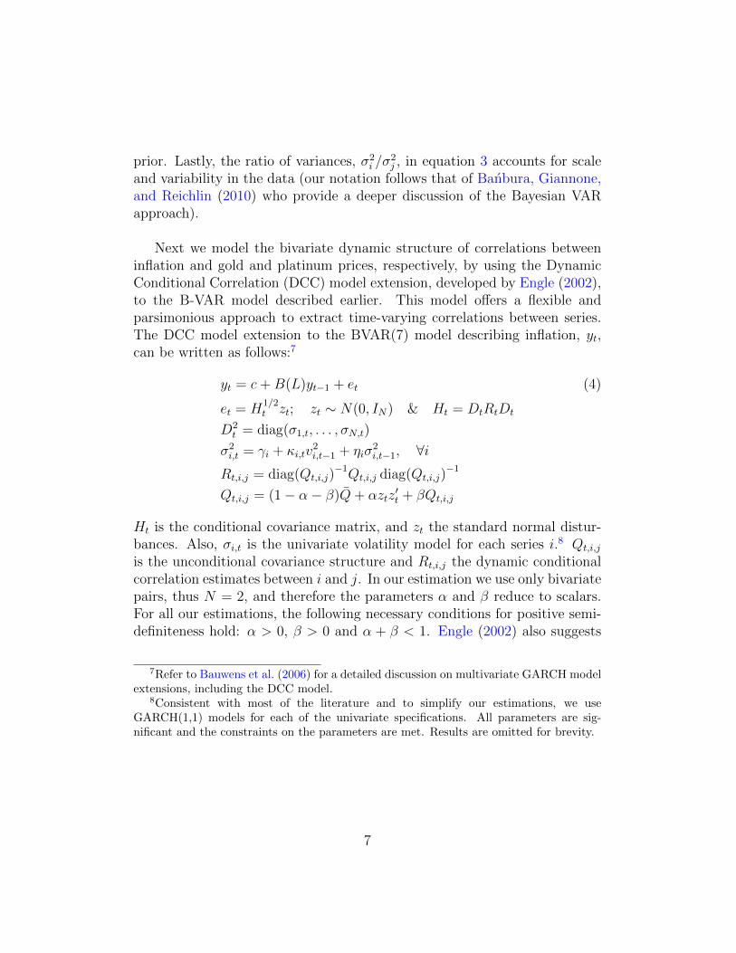
Next we model the bivariate dynamic structure of correlations betweeninflation and gold and platinum prices, respectively, by using the DynamicConditional Correlation (DCC) model extension, developed by Engle (2002),to the B-VAR model described earlier. This model offers a flexible andparsimonious approach to extract time-varying correlations between series.The DCC model extension to the BVAR(7) model describing inflation, yt,can be written as follows:7

yt = c+B(L)yt−1 + et (4)

et = H1/2t zt; zt ∼ N(0, IN) & Ht = DtRtDt

D2t = diag(σ1,t, . . . , σN,t)

σ2i,t = γi + κi,tv

2i,t−1 + ηiσ

2i,t−1, ∀i

Rt,i,j = diag(Qt,i,j)−1Qt,i,j diag(Qt,i,j)

−1

Qt,i,j = (1− α− β)Q+ αztz′t + βQt,i,j

Ht is the conditional covariance matrix, and zt the standard normal distur-bances. Also, σi,t is the univariate volatility model for each series i.8 Qt,i,j

is the unconditional covariance structure and Rt,i,j the dynamic conditionalcorrelation estimates between i and j. In our estimation we use only bivariatepairs, thus N = 2, and therefore the parameters α and β reduce to scalars.For all our estimations, the following necessary conditions for positive semi-definiteness hold: α > 0, β > 0 and α + β < 1. Engle (2002) also suggests

7Refer to Bauwens et al. (2006) for a detailed discussion on multivariate GARCH modelextensions, including the DCC model.

8Consistent with most of the literature and to simplify our estimations, we useGARCH(1,1) models for each of the univariate specifications. All parameters are sig-nificant and the constraints on the parameters are met. Results are omitted for brevity.

7

specifying a log-likelihood for the model in 4 defined as:

ln(L) = −1

2

T∑t−1

[N ln(2π) + 2 ln|Dt|+ e′tD

−1t D−1

t et

− εtε′t + ln|Rt,i,j|+ ε′tR−1t,i,jεt

](5)

We then perform Bayesian estimation of the DCC model parameters to over-come one of the major drawbacks of this approach, its static correlationstructure. This is done using the Metropolis Hastings algorithm for estimat-ing the DCC parameters, similar to that suggested by Della Corte, Sarno,and Tsiakas (2010).9

After fitting both the BVAR and BVAR-BDCC GARCH models, we pro-ceed to generate point and density inflation forecasts. We compute h =1, 2, ..., 24 step ahead monthly forecasts for each of the models discussed onan iterative basis, in order to compare it to RW and AR forecasts. Thecomparisons are made based on the following statistics. Firstly, we comparethe point forecast estimates using the familiar Root Mean Squared Error(RMSE) statistic, which is given as:

RMSEk,h =

√√√√ t−h∑t=

¯t

(yt+h,h − yt+h,k)2

t∗(6)

where t∗ = t− h+¯t+ 1,

¯t is the beginning and t the end of the forecasting

period, and yt and yt the forecast and true values, respectively. Using thismeasure, we can assess which model provides the best point forecast estimate.

We also compare density forecasts using the Logarithmic Score statistic,LS, as discussed in detail in Mitchell and Hall (2005, 2007). The usefulness ofevaluating density forecassts in addition to point estimates has been outlinedby Tay and Wallis (2000), who argue that density measures allows for a fullimpression of the uncertainty associated with forecasts. In our analysis, itprovides an estimate of the probability distribution of future values for infla-tion as predicted by each model. Following the discussion in Mitchell and Hall

9For a detailed discussion of the Bayesian DCC approach, the reader is referred toDella Corte et al. (2010), while Lombardi and Ravazzolo (2013) provides a good conciseoverview of this approach in their appendix.

8

(2005), density forecasts can be combined using “optimal” weights. Theseoptimal weights minimize the distance between canditate model k ’s com-bined density forecasts, p(yk,T+1|y1:t), and the true densities, p(yk,T+1|y1:t),which are unknown. In doing so, the Kullback-Leibler Information Criterion(KLIC) measure is used to obtain these optimal weights for model k, whichminimize the distance between the combined and true densities (Mitchell andHall, 2007, p.4):

KLICk,t+h =

∫p(yt+h|y1:t) ln

p(yt+h|y1:t)

p(yt+h|y1:t)(7)

KLICk,t+h = Et (ln p(yt+h|y1:t)− ln p(yt+h|y1:t) (8)

where Et = E(.|Ft) is the conditional expectation given information set Ft.The smaller the distance in 8, the closer the density forecast of model k isto the “true density”. It then follows that under some regularity conditions,the criterion can be rewritten as10:

KLICk,t+h =1

t∗

t−h∑t=

¯t

(ln p(yt+h|y1:t)− ln p(yt+h|y1:t)) (9)

where t∗ corresponds to our out-of-sample range discussed in Section 5, andthe sample statistic, 1

t∗

∑(.), is used as an unbiased estimate of Et. Intu-

itively, the KLIC statistic thus chooses the model which, on average, givesthe highest probability to the events which occured (or the model having thehighest posterior probability). Minimizing the KLIC statistic, is equivalentto maximizing the second part of equation 9, which is the Logarithmic Scorestatistic. This follows as the “true” density is not observable, yet we neednot know lnp(yt+h|y1:t) in order to compare two models’ density forecast fits,as it would be relative to the same “true” density. Thus, we have:

LSk = − 1

t∗

t−h∑t=

¯t

ln p(yt+h|y1:t) (10)

In order to assess the significance of the model performance in our out-of-sample point forecast estimates, we use Diebold and Mariano (1995)’s (DM)

10C.f. Mitchell and Hall (2007, p. 4). Here we follow the notation of Lombardi andRavazzolo (2012)

9

test. The test evaluates the null hypothesis of equal forecasting accuracy ofeach bivariate model pair compared to the alternative that one of the modelsoutperformed the other in terms of forecasting accuracy. We use the smallsample adjusted version of the DM test, as suggested by Harvey, Leybourne,and Newbold (1997), which is a pairwise test that adjusts the DM, and isdefined as follows:

E[di,t] = E[Λw1,t − Λw

2,t] = 0 (11)

and then following Harvey et al. (1997), we adjust it as follows:

Adjusted DM =

(t∗ + 1− 2h+ t∗−1h(h− 1)

t∗

)1/2

V (di−1/2)di (12)

where Λwi,t = yt − yi,t is the weighted loss function as described in Dijk and

Franses (2003), h being the forecast horizon, and V (di−1/2) the estimated

variance of series di,t. The Adjusted DM test statistic is then comparedto critical values from the t-distribution with degrees of freedom t∗ − 1.In the adjusted DM above, we use Newey-West HAC consistent varianceestimators. The Bandwidth for the Newey-West estimator is then selectedusing Andrews’ (1991) automatic bandwidth selector.11

In order to compare model significance in terms of density forecasts, wefollow a similar yet somewhat adjusted approach to the above, as outlined inMitchell and Hall (2005). The null hypothesis of equal density forecast is:

E[di,t] = 0⇒ KLIC = 0 (13)

with the sample mean d defined as (Mitchell and Hall, 2005, p.1004):

d = KLIC =1

t∗

t−h∑t=

¯t

[ln pt(z1t)∗ − lnφ(z∗1t)] (14)

with z1t =∫ yt−∞ gu(u)du, and z∗1t = Φ−1z1t, where φ(·) is the standard normal

density function and Φ the c.d.f of the standard normal. As noted in Mitchell

11For details, see: Andrews, D. W. (1991). Heteroskedasticity and autocorrelation con-sistent covariance matrix estimation. Econometrica: Journal of the Econometric Society,817-858.

10

and Hall (2005), testing for the departure of z1tt∗t=1 from i.i.d N(0, 1)12 is

equivalent to testing the departure of the forecasted density from the truedensity, p(yt+h|y1:t), as defined earlier.

In order to test equation 14, we follow Mitchell and Hall (2005) in usingthe central limit theorem and, under appropriate assumtions, testing thedistribution:

√t∗(d− E(dt))→ N(0,Ω) (15)

where the general representation for the covariance matrix, Ω, is given inWest (1996), and reduces to the long run covariance matrix, Sd. This is,in turn, associated with dt in that it is 2π times the spectral density ofdt − E(dt) at zero frequency (Mitchell and Hall, 2005).13 This test thenreduces to the small sample corrected and HAC robust DM test if dt testedfor point error forecasts. As argued in Mitchell and Hall (2005), such testingfor the significance of departures of z∗1t from N(0, 1), is both easier and moresensible than testing the distance of density forecasts as defined in equation9.

The results of both the point and density forecast tests are reported inTable A.4 and discussed in Section 5.

4. Data

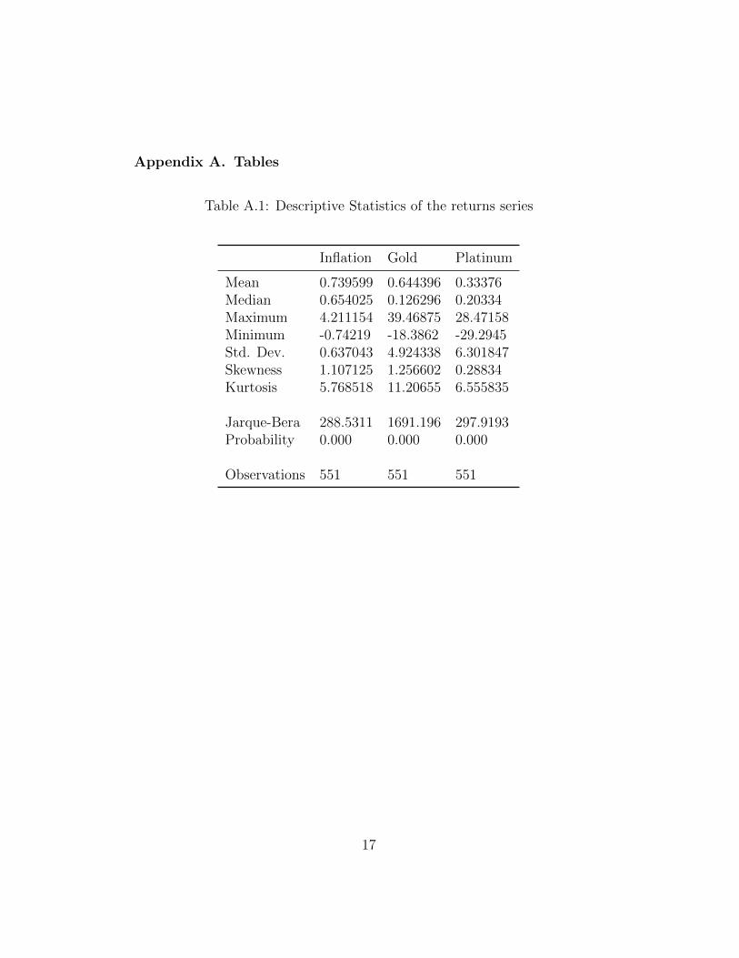
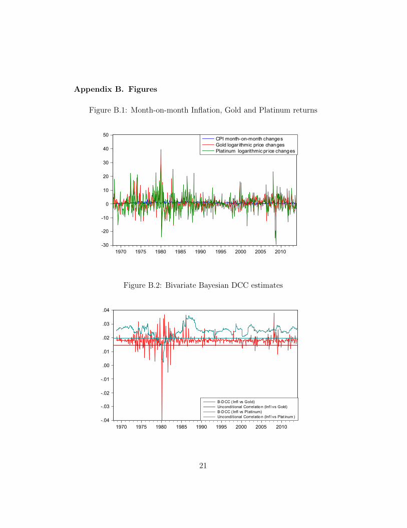
In this study we use monthly data for the period 1968M2 to 2013M12,for SA inflation (CPI) as well as gold and platinum price indexes. Our datafor CPI inflation was obtained from the Global Financial database, while theplatinum and gold price series were obtained from www.kitco.com. We usedthe dollar prices for both gold and platinum, firstly as these metals are tradedglobally in dollars, and secondly in order to avoid exchange rate effects oninflation in our estimates. Table A.1 shows the descriptive statistics of thereturns to each of the series14, and figure B.1 graphs the month-on-monthinflation and continuously compounded returns for the gold- and platinumseries. From both Table A.1 and figure B.1 it is clear that platinum prices

12Which is, in turn, equivalent to testing z1t’s departure from i.i.d. U(0, 1)13More details of estimating Sd follows in Mitchell and Hall (2005, p. 1004 - 1005).14For each price index, we use the first difference of the logarithmic transformation to

achieve stationarity.

11

show the greatest variability, while both metals series show far more pricevariability than prices on aggregate.

Also, all the price returns series reject the null of normality, and displayexcess kurtosis and skewness. Finally, all three series show logarithmicallydifferenced stationarity, as can be seen from the Augmented Dickey-Fuller(ADF) and Philips-Perron (PP) tests contained in the appendix (see TableA.2). Although less convincing for inflation using the standard ADF test,the PP test indeed shows clear evidence of stationarity.

Figure B.2 in the appendix compares the bivariate Bayesian DynamicConditional Correlations (B-DCC) between inflation and the respective met-als price series, relative to their unconditional sample correlation. From thefigures it is clear that the unconditional estimates for both are consistentlylower than for the dynamic estimates. We also note from these figures thatthe correlation between the inflation series and the metals returns series typ-ically display relatively muted and positive correlations. As such, we requirethe point and density forecast evaluation results to be able to infer whethermetals price series should indeed be considered as important inputs to infla-tion forecasts.

5. Results

Table A.3 shows both the point and density out-of-sample forecast accu-racy tests for the B-VAR and BVAR B-DCC models discussed in Section 3.The period considered ranges from 2000M01 – 2013m12, which correspondsto the period of inflation targeting.

From Table A.3, it is clear that the results for the point forecasts suggestthat the AR(7) model is particularly difficult to improve upon. This is con-sistent with the findings of Lombardi and Ravazzolo (2012) and most otherstudies that similarly have difficulty in finding more accurate point estimatesthan the autoregressive models. Table A.4 confirms the significance of theout performance relative to both BDCC estimates, using gold and platinumas bivariate inputs, in terms of point forecasts.

Nonetheless, as argued in Section 3, we should be more interested in theability of models to provide accurate density forecast estimates. This followsas it is a more holistic approach to assessing the model’s ability to predictfuture price movements. The LS statistic in Table A.3, in contrast to thefindings for point forecasts, shows that the B-DCC models consistently pro-vide improved density forecasts of inflation at every horizon versus all the

12

other models. Also, the B-VAR for both metals series also provide improveddensity forecasts versus the RW and AR(7) benchmarks. Collectively, thisimplies that at all horizons we see that controlling for dynamic correlations,using BDCC extensions to the BVAR model, improves density forecasts. Wealso deduce that metals price series contain information which improves in-flation forecasting power at all horizons as well. The improvement from theBVAR as a result of the addition of BDCC estimates, are more significant asthe forward horizon increases, as can be seen from Table A.4. For all densityforecast horizons we see that the BDCC models provide significantly moreaccurate estimates than the RW model, while for most AR(7) horizons thetests suggest significant improvements at longer horizons.

Our results can then be summarized as follows. Firstly, metals price se-ries, proxied for by gold and platinum prices, provide useful information inorder to improve density forecasts of inflation based solely on past inflationinformation. Secondly, improving point forecast estimates from naive mod-els remain an elusive, albeit less informative, exercise. Lastly, we see thatcontrolling for the dynamic relationship between inflation and other priceseries used as model inputs, leads to statistically significant improvements indensity forecasts.

6. Conclusion

This paper studies the dynamic relationship between inflation and metalsprice series for South Africa, for the period 1968 – 2013. It tests two hypothe-ses. First, whether metals series provide useful information in the point anddensity out-of-sample forecasting of inflation for the period since adoptinginflation targeting. Secondly, we test whether controlling for the dynamicconditional co-movements between the bivariate pairs of price series yieldsimproved forecasting perfomance. This is done using a bivariate BayesianVAR Bayesian DCC-GARCH model, and comparing the out-of-sample fore-casting performances at various horizons. To achieve this, we make use ofthe RMSE statistics for point forecast estimates, the Log-Score statistic fordensity forecasts and a modified version of the Diebold and Mariano (1995)test and the Mitchell and Hall (2005) test to evaluate the statistical signifi-cance of model forecast out-performance for both point and density forecasts,respectively.

13

Our findings can be summarized as follows. We find that improving pointforecasts of naive Random Walk and Autoregressive models for the inflationseries, using our dynamic model estimates, remain an elusive exercise. This,we argue, is of less importance relative to the more informative density fore-casts, for which we find significantly improved forecasts of inflation for boththe BVAR and BDCC models over the naive benchmarks. Particularly, wefind that controlling for dynamic correlations between the series leads to su-perior density forecasts at all horizons. This allows us to make several conclu-sions. Firstly, that including metals price series as inputs to inflation modelsleads to improved density forecasts. Secondly, controlling for the dynamicrelationship between the included price series and inflation similarly leadsto significantly improved forecasts. This implies that forecasters should con-sider the importance of metals series in describing the movements of pricesin South Africa, while advanced models studying future price movementsshould ideally control for the dynamic relationships of the series considered.Our Bayesian estimates allow the dynamic structure of correlation to be moreflexible and adjustable relative to the standard DCC estimates typically usedin the literature.

References

Banbura, M., D. Giannone, and L. Reichlin (2010). Large bayesian vectorauto regressions. Journal of Applied Econometrics 25 (1), 71–92.

Baumeister, C. and L. Kilian (2012). Real-time forecasts of the real price ofoil. Journal of Business & Economic Statistics 30 (2), 326–336.

Bauwens, L., S. Laurent, and J. V. Rombouts (2006). Multivariate garchmodels: a survey. Journal of applied econometrics 21 (1), 79–109.

Bean, C. (2004). Inflation targeting: the uk experience. Perspektiven derWirtschaftspolitik 5 (4), 405–421.

Bernanke, B. and M. Gertler (2000). Monetary policy and asset price volatil-ity. Technical report, National bureau of economic research.

Bernanke, B. S. and M. Gertler (2001). Should central banks respond tomovements in asset prices? american economic review , 253–257.

14

Cecchetti, S. G., H. Genberg, and S. Wadhwani (2002). Asset prices in aflexible inflation targeting framework. Technical report, National Bureauof Economic Research.

Chen, Y.-c., S. J. Turnovsky, and E. Zivot (2011). Forecasting inflation usingcommodity price aggregates. Technical report, University of Washington,Department of Economics.

Della Corte, P., L. Sarno, and I. Tsiakas (2010). Correlation timing in assetallocation with bayesian learning. Technical report, Warwick BusinessSchool,.

Diebold, F. X. and R. S. Mariano (1995). Comparing predictive accuracy.Journal of Business & Economic Statistics 13 (3).

Dijk, D. and P. H. Franses (2003). Selecting a nonlinear time series modelusing weighted tests of equal forecast accuracy*. Oxford Bulletin of Eco-nomics and Statistics 65 (s1), 727–744.

Doan, T., R. Litterman, and C. Sims (1984). Forecasting and conditionalprojection using realistic prior distributions. Econometric reviews 3 (1),1–100.

Engle, R. (2002). Dynamic conditional correlation: A simple class of mul-tivariate generalized autoregressive conditional heteroskedasticity models.Journal of Business & Economic Statistics 20 (3), 339–350.

Fuhrer, J. and G. Moore (1992). Monetary policy rules and the indicatorproperties of asset prices. Journal of Monetary Economics 29 (2), 303–336.

Furlong, F. and R. Ingenito (1996). Commodity prices and inflation. Eco-nomic Review-Federal Reserve Bank of San Francisco, 27–47.

Gospodinov, N. and S. Ng (2013). Commodity prices, convenience yields,and inflation. The Review of Economics and Statistics 95 (1), 206–219.

Harvey, D., S. Leybourne, and P. Newbold (1997). Testing the equality ofprediction mean squared errors. International Journal of forecasting 13 (2),281–291.

15

Hooker, M. A. (2002). Are oil shocks inflationary?: Asymmetric and nonlin-ear specifications versus changes in regime. Journal of Money, Credit, andBanking 34 (2), 540–561.

Kadiyala, K. and S. Karlsson (1997). Numerical methods for estimation andinference in bayesian var-models. Journal of Applied Econometrics 12 (2),99–132.

Korobilis, D. (2013). Var forecasting using bayesian variable selection. Jour-nal of Applied Econometrics 28 (2), 204–230.

Litterman, R. B. (1986). Forecasting with bayesian vector autoregressionsfiveyears of experience. Journal of Business & Economic Statistics 4 (1), 25–38.

Lombardi, M. J. and F. Ravazzolo (2012). Oil price density forecasts: ex-ploring the linkages with stock markets.

Lombardi, M. J. and F. Ravazzolo (2013). On the correlation between com-modity and equity returns: implications for portfolio allocation. BIS Work-ing Paper .

Mitchell, J. and S. G. Hall (2005). Evaluating, comparing and combiningdensity forecasts using the klic with an application to the bank of eng-land and niesr fancharts of inflation*. Oxford bulletin of economics andstatistics 67 (s1), 995–1033.

Mitchell, J. and S. G. Hall (2007). Combining density forecasts. InternationalJournal of Forecasting 23 (1), 1–13.

Stock, J. H. and M. W. Watson (2001). Forecasting output and inflation:the role of asset prices. Technical report, National Bureau of EconomicResearch.

Tay, A. S. and K. F. Wallis (2000). Density forecasting: a survey. Journalof forecasting 19 (4), 235–254.

Ustyugova, Y. and G. Gelos (2012). Inflation responses to commodity priceshocks-how and why do countries differ? IMF Working Paper .

West, K. D. (1996). Asymptotic inference about predictive ability. Econo-metrica: Journal of the Econometric Society , 1067–1084.

16

Appendix A. Tables

Table A.1: Descriptive Statistics of the returns series

Inflation Gold Platinum

Mean 0.739599 0.644396 0.33376Median 0.654025 0.126296 0.20334Maximum 4.211154 39.46875 28.47158Minimum -0.74219 -18.3862 -29.2945Std. Dev. 0.637043 4.924338 6.301847Skewness 1.107125 1.256602 0.28834Kurtosis 5.768518 11.20655 6.555835

Jarque-Bera 288.5311 1691.196 297.9193Probability 0.000 0.000 0.000

Observations 551 551 551

17

Table A.2: Tests for Unit Roots

Inflation t-Statistic Prob.

Augmented Dickey-Fuller test statistic -2.774 0.0628Test critical values: 1% level -3.442

5% level -2.86710% level -2.57

Gold Returns t-Statistic Prob.

Augmented Dickey-Fuller test statistic -15.97 0.000Test critical values: 1% level -3.442

5% level -2.86710% level -2.57

Platinum Returns t-Statistic Prob.

Augmented Dickey-Fuller test statistic -18.26 0.000Test critical values: 1% level -3.442

5% level -2.86710% level -2.57

Inflation Adj. t-Statistic Prob.

Phillips-Perron test statistic -22.89 0.000Test critical values: 1% level -3.442

5% level -2.86710% level -2.57

Gold Returns Adj. t-Statistic Prob.

Phillips-Perron test statistic -17.51 0.000Test critical values: 1% level -3.442

5% level -2.86710% level -2.57

Platinum Returns Adj. t-Statistic Prob.

Phillips-Perron test statistic -18.22 0.000Test critical values: 1% level -3.442

5% level -2.86710% level -2.57

Both the Aumented Dickey-Fuller and Phillips-Perron tests useMacKinnon’s (1996) one-sided p-values. The latter test alsoemploys the Newey-West automatic bandwidth selector andBartletts’s kernel.

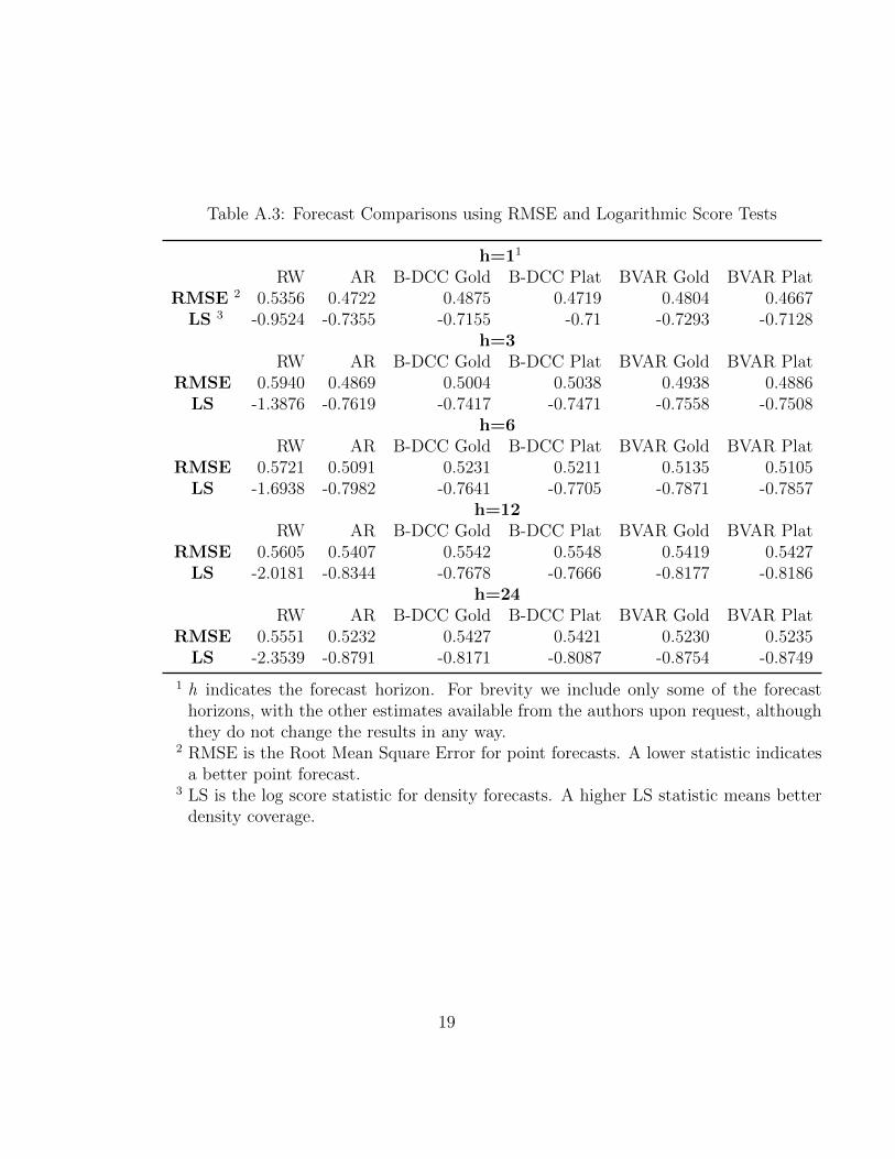
Table A.3: Forecast Comparisons using RMSE and Logarithmic Score Tests

h=11

RW AR B-DCC Gold B-DCC Plat BVAR Gold BVAR PlatRMSE 2 0.5356 0.4722 0.4875 0.4719 0.4804 0.4667LS 3 -0.9524 -0.7355 -0.7155 -0.71 -0.7293 -0.7128

h=3RW AR B-DCC Gold B-DCC Plat BVAR Gold BVAR Plat

RMSE 0.5940 0.4869 0.5004 0.5038 0.4938 0.4886LS -1.3876 -0.7619 -0.7417 -0.7471 -0.7558 -0.7508

h=6RW AR B-DCC Gold B-DCC Plat BVAR Gold BVAR Plat

RMSE 0.5721 0.5091 0.5231 0.5211 0.5135 0.5105LS -1.6938 -0.7982 -0.7641 -0.7705 -0.7871 -0.7857

h=12RW AR B-DCC Gold B-DCC Plat BVAR Gold BVAR Plat

RMSE 0.5605 0.5407 0.5542 0.5548 0.5419 0.5427LS -2.0181 -0.8344 -0.7678 -0.7666 -0.8177 -0.8186

h=24RW AR B-DCC Gold B-DCC Plat BVAR Gold BVAR Plat

RMSE 0.5551 0.5232 0.5427 0.5421 0.5230 0.5235LS -2.3539 -0.8791 -0.8171 -0.8087 -0.8754 -0.8749

1 h indicates the forecast horizon. For brevity we include only some of the forecasthorizons, with the other estimates available from the authors upon request, althoughthey do not change the results in any way.

2 RMSE is the Root Mean Square Error for point forecasts. A lower statistic indicatesa better point forecast.

3 LS is the log score statistic for density forecasts. A higher LS statistic means betterdensity coverage.

19

Table A.4: Point and Density Forecast Accuracy

Gold point forecasts1

horizon RW vs. BDCC AR vs. BDCC BDCC vs. BVAR1 1.149 -2.429** 2.139**3 2.175** -1.584 1.5246 1.291 -1.797* 2.567**12 0.135 -3.544*** 3.313***24 0.214 -4.216*** 4.249***

Gold density forecasts2

horizon RW vs. BDCC AR vs. BDCC BDCC vs. BVAR1 -3.949*** -0.232 0.0613 -9.286*** -0.46 0.3286 -10.999*** -1.141 1.13712 -12.844*** -2.883*** 2.901***24 -35.826*** -1.851* 1.604

Platinum point forecasts

horizon RW vs. BDCC AR vs. BDCC BDCC vs. BVAR1 1.611 0.052 1.563 2.205** -3.208*** 3.747***6 1.343 -2.104** 2.146**12 0.12 -3.493*** 3.427***24 0.222 -2.880*** 2.916***

Platinum density forecasts

horizon RW vs. BDCC AR vs. BDCC BDCC vs. BVAR1 -4.723*** -0.605 -0.2713 -9.703*** -0.448 0.0326 -11.122*** -1.216 0.90412 -12.480*** -2.789*** 2.942***24 -35.687*** -1.942* 1.696*

1 The adjusted Diebold-Mariano (DM) test is used for the point forecast evalua-tion. A positive and significant value implies model 2 provides a signficantlybetter forecast, and vice versa.

2 The Mitchell and Hall (2005) test is used for density forecast evaluation. A neg-ative and significant value implies model 2 provides significantly better densityforecast.*, *, and *** denote significance at 10%, 5% and 1%, respectively.

Appendix B. Figures

Figure B.1: Month-on-month Inflation, Gold and Platinum returns

-30

-20

-10

0

10

20

30

40

50

1970 1975 1980 1985 1990 1995 2000 2005 2010

CPI month-on-month changesGold logar ithmic price changesPlatinum logarithmic pr ice changes

Figure B.2: Bivariate Bayesian DCC estimates

-.04

-.03

-.02

-.01

.00

.01

.02

.03

.04

1970 1975 1980 1985 1990 1995 2000 2005 2010

B-DCC (Infl vs Gold)Unconditional Correlatio n (Inf l vs Gold)B-DCC (Infl vs Platinum)Unconditional Correlatio n (Inf l vs Plat inum )

21