1

Real Options Analysis

Office Tower BuildingPortfolio Presentation

Fall 2008ESD.71

Professor: Richard de NeufvillePresented by: Charbel Rizk

Introduction

2

• Application of Real Options in construction field• Time between design and completion relatively long• Large Investment, expected long life cycle• Office Building Tower – Based on real projects• 2 types of offices:o For Investor’s Use o For Sale

• Project completion around 2000• Lack of space in 2006

www.manenterprise.com

Objective & Procedure

3

Analyze project based on tools and method learned in class: • Identify main uncertainties in design:

o Investor’s Office requiremento Market Demand (Offices, Stores)

- For simplicity considered only Investor’s office demand • Identify different scenarios: -Low; -Medium; -High• Find possible (feasible) options to be added:

o Original: Fixed, deterministic designo Re-buy Optiono Option to Add Floors

• Evaluate all designso Evaluation based on expected monetary valueo Two stages decision analysiso Lattice decision analysis

Summary of Designs

4

• Fixed design: (3 floors for investor’s use)o 7 Floors office towero 4 Floors for sale

• Flexible contract: (2, or 3, or 4 floors for investor’s use)o 7 Floors office towero 3 Floors for saleo 2 Other floors for sale with option to Re-buy

• Flexible design: (2, or 3, or 4 floors for investor’s use)

o Start with 6 floors office towero 4 Floors for saleo Option to add 1 or 2 Floorso Maximum number of floors is higher due to lower risk

Assumptions (Simplifying) & Expected Demand

5

• Floors to be sold will be sold upon completion• Time for execution 1 year• Construction cost paid at t=0• r=10%• i=2%• Assumed Cost of not having when required based on lost

opportunities• Benefits are not included (Since using incremental NPV’s) • Area per floor= 220m2

General & Particular Costs

6

• General, defined per unit applicable to all designs - Construction Cost

- Maintenance- Running & Fees(Power, Ventilating, etc…)- Cost of Lacking space

• Particular, unit rate differs or not applicable to all designs- Permit cost- Option Cost

a) Allow for Re-buy option in contractb) Allow for adding floors (thicker columns, etc…)

- Strike pricec) Re-buying floor/sd) Adding floor/s

Two Stages Decision Analysis

7

• Probabilities are shown below

• Flexible contract or design : Add option to change decision

Year 0(Actual)

Sc Bet Yrs0 & 5

Year 5(Forecast) Prob(0->5)

Sc Bet Yrs5 & 10

Year 10(Forecast)

Prob(5->10)/Year(0->5)

Low 2 0.6Low 2 0.15 Medium 2 0.3

High 3 0.1Low 3 0.15

Medium 3 0.4 Medium 4 0.4High 4 0.45Low 4 0.05

High 4 0.45 Medium 4 0.25High 4 0.7

2

Year 5 Year 5

Two Stages Decision Analysis (Cont.)

8

• NPV calculation for each end node• ENPV calculation• Pruning based on maximize ENPV

Status Probability Best Decision Value Expected V. Best Decision Value Expected V. Best Decision Value Expected V.Low - Low 0.09 Can't Do antg -2,227,429 Do Nothing -1,067,182 Do Nothing -1,143,182

Low- Medium 0.045 Can't Do antg -2,227,429 Do Nothing -1,067,182 Do Nothing -1,143,182Low - High 0.015 Can't Do antg -1,938,965 Do Nothing -1,355,645 Do Nothing -1,431,645

Medium - Low 0.06 Can't Do antg -1,938,965 Re-Buy 1 Fl -1,337,283 Add 1 Floor -296,796Medium - Medium 0.16 Can't Do antg -2,227,429 Re-Buy 1 Fl -1,625,747 Add 1 Floor -585,260

Medium - High 0.18 Can't Do antg -2,227,429 Re-Buy 1 Fl -1,625,747 Add 1 Floor -585,260

High - Low 0.0225 Can't Do antg -2,227,429 Re-Buy 1 Fl -1,625,747 Add 2 Floors -550,411High - Medium 0.1125 Can't Do antg -2,227,429 Re-Buy 1 Fl -1,625,747 Add 2 Floors -550,411

High - High 0.315 Can't Do antg -2,227,429 Re-Buy 1 Fl -1,625,747 Add 2 Floors -550,411

Flexible ContractFixed Design Flexible Design

-2,205,794 -1,528,981 -640,285

De

sig

n T

yp

e

Year 5 Action at year 5 Year 10 Options

EV At 5Decide ifPossible

@ 5

Decsision@ Year 5

If Scenario

EV@ 0

If DesignType

High Not Applicable Low -2,227,429High Not Applicable Medium -2,227,429High Not Applicable High -2,227,429

Medium Not Applicable Low -1,938,965Medium Not Applicable Medium -2,227,429Medium Not Applicable High -2,227,429

Low Not Applicable Low -2,227,429Low Not Applicable Medium -2,227,429Low Not Applicable High -1,938,965

Fix

ed

De

sig

n

-2,205,794-2,205,794

-2,227,429

-2,184,159

-2,198,583

NothingTo

Chose

Two Stages Decision Analysis (Cont.)

9

Best Strategy & VARG:At t=0 choose flexible design

a) If demand during first period Was high => Add 2 Floorsb) If demand during first period was Medium => Add 2 Floorsc) If demand during first period was Low => Don’t Add Floors

-2,500.00 -2,000.00 -1,500.00 -1,000.00 -500.00 0.00 500.000

0.2

0.4

0.6

0.8

1

1.2

VARG Chart

Fixed DesignFlexible ContractFlexible DesignEV Fixed DesignEV Flexible ContractEV Flexible Design

Values in 1,000$

Prob

abili

ties

Lattice Decision Analysis

10

• Determine: u, d, & p using:- Maximum Value= S u u => u= Sqrt(Max/S)- Minimum Value= S d d => d= Sqrt(Min/S) - Most Likely= p2 * (S u u ) + 2*p*(1-p)*(S u d) + (1-p)2 * (S d d)

• Results: - u= 1.4142- d= 1.0000- p= 0.8494

P=0 P=1 P=2 P=0 P=1 P=2

S u u Max p2

S u pS S u d p=1 2 * p * (1-p)

S d (1-p)

S d d Min (1-p)2

Outcome Latice: Probability Lattice:

Lattice Decision Analysis (Cont.)

11

• Resulting outcome & probability lattice:

• Probability distribution function:

Data for PDF:

P=0 P=1(5 Yrs) P=2 (10 Yrs) P=3(15 Yrs) P=4(20 Yrs) P=5(25Yrs) P=0 P=1(5 Yrs) P=2 (10 Yrs) P=3(15 Yrs) P=4(20 Yrs) P=5(25Yrs)2.00 2.83 4.00 5.66 8.00 11.31 1.00 0.85 0.72 0.61 0.52 0.44

2.00 2.83 4.00 5.66 8.00 0.15 0.26 0.33 0.37 0.392.00 2.83 4.00 5.66 0.02 0.06 0.10 0.14

2.00 2.83 4.00 0.00 0.01 0.022.00 2.83 0.00 0.00

2.00 0.00

Probability LatticeOutcome Lattice

0.00 2.00 4.00 6.00 8.00 10.0012.0014.0016.0018.000.00

0.05

0.10

0.15

0.20

0.25

0.30

0.35

0.40

0.45

PDF for Lattice

Outcome

Pro

bab

ilit

yOutcome Prob Rank

c-1 11.31 0.44 5.00c-2 8.00 0.39 4.00c-3 5.66 0.14 3.00c-4 4.00 0.02 2.00c-5 2.83 0.00 1.00c-6 2.00 0.00 0.00

Lattice Decision Analysis (Cont.)

12

• Option evaluation:- Prepare cash flow per state & stage for each design- Find ENPV for each design:

ENPV = Cash Flow Lattice * Probability Lattice

- Decison Lattice (Strategy):

P=0 P=1 P=2 P=3 P=4 P=5 P=0 P=1 P=2 P=3 P=4 P=5Cash Flow (566.00) (4469.67) (4687.05) (7689.60) (7689.60) (7689.60) ENPV (Cash Flow) (9376.07) (13617.63) (14267.18) (15428.91) (12464.23) (7689.60)Flexibility (6082.43) (7332.96) (7689.60) (7689.60) (7689.60) Flexibility (17410.70) (17360.39) (15428.91) (12464.23) (7689.60)

2 Floors Added (9978.88) (12030.50) (7689.60) (7689.60) 2 Floors Added (23231.25) (20213.55) (12464.23) (7689.60)Dynamic programming (16371.40) (12030.50) (7689.60) Dynamic programming (27715.82) (17210.94) (7689.60)

approach (16371.40) (12030.50) approach (24247.20) (12030.50)(16371.40) (16371.40)

Flexible Design ENPV in 1,000 of $ Expanded (Taking All 4 Floors)Flexible Design Cash Flow in 1,000 of $ Expanded (Taking All 4 Floors)

P=0 P=1 P=2 P=3 P=4 P=5Excercise CALL Add 2 Fl. Add 2 Fl. Add 2 Fl. Add 2 Fl. Add 2 Fl.

OPTION ? Don't Add Add 2 Fl. Add 2 Fl. Add 2 Fl.Don't Add Add 2 Fl. Add 2 Fl.

Don't Add Don't AddDon't Add

Lattice Decision Analysis (Cont.)

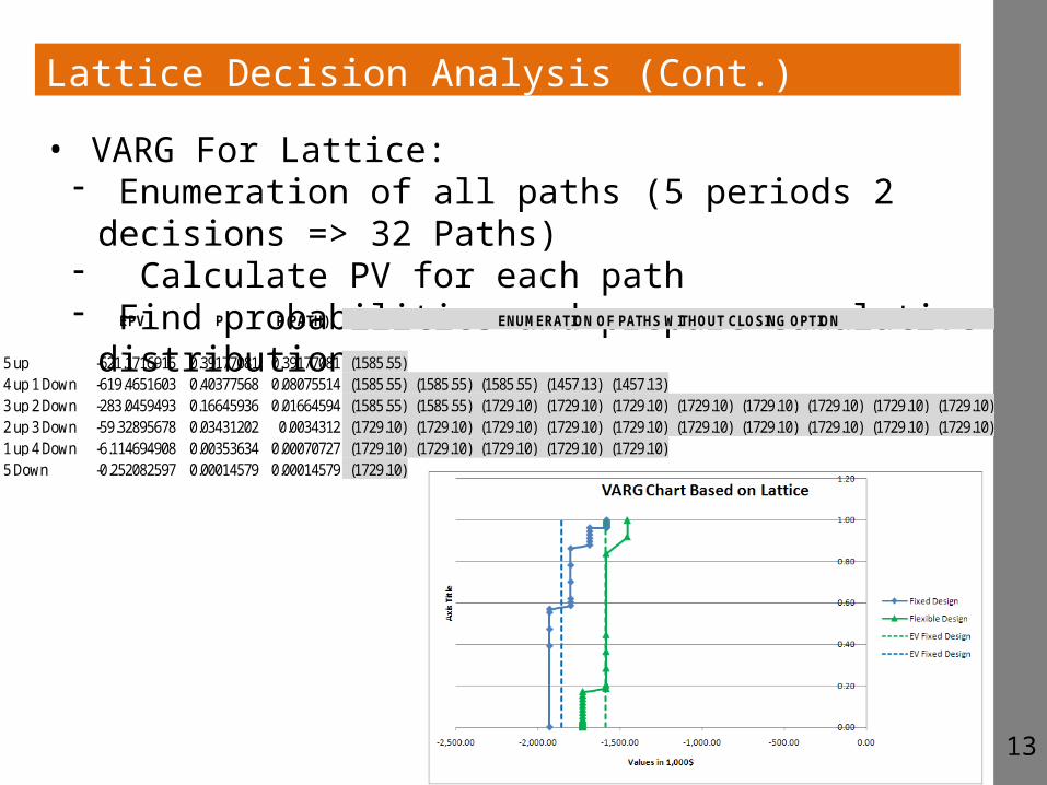
13

• VARG For Lattice:- Enumeration of all paths (5 periods 2 decisions => 32 Paths)- Calculate PV for each path- Find probabilities and prepare cumulative distribution

EPV P P(PATH)

5 up -621.1716915 0.39177081 0.39177081 (1585.55)4 up 1 Down -619.4651603 0.40377568 0.08075514 (1585.55) (1585.55) (1585.55) (1457.13) (1457.13)3 up 2 Down -283.0459493 0.16645936 0.01664594 (1585.55) (1585.55) (1729.10) (1729.10) (1729.10) (1729.10) (1729.10) (1729.10) (1729.10) (1729.10)2 up 3 Down -59.32895678 0.03431202 0.0034312 (1729.10) (1729.10) (1729.10) (1729.10) (1729.10) (1729.10) (1729.10) (1729.10) (1729.10) (1729.10)1 up 4 Down -6.114694908 0.00353634 0.00070727 (1729.10) (1729.10) (1729.10) (1729.10) (1729.10)5 Down -0.252082597 0.00014579 0.00014579 (1729.10)

ENUMERATION OF PATHS WITHOUT CLOSING OPTION

Conclusions

14

• Demand variance was small and still:- Based on decision trees: Flexible design was best alternative- Based on lattice analysis: Option value above $ 1 M

• All values are not accurate, they are upper & lower bounds only• Designers should take uncertainty into consideration, especially

with the availability of all new tools • Discussion in this paper is based on NPV analysis only• Other tools metrics can also be taken into consideration for

example:- Benefit to cost ratio- Payback period- Risks- Range of outcomes (maximum, minimum)

15

Thank you For Your Time

Comments?Questions?