1 recent developments in tree induction for kdd « towards soft tree induction » louis wehenkel...
Post on 18-Dec-2015
216 views
TRANSCRIPT

1
Recent developments in tree induction for KDD
« Towards soft tree induction »
Louis WEHENKELUniversity of Liège – Belgium
Department of Electrical and Computer Engineering

2
A. Supervised learning (notation)
x = (x1,…,xm) vector of input variables (numerical and/or symbolic)
y single output variable Symbolic : classification problem Numeric : regression problem
LS = ((x1,y1),…,(xN,yN)), sample of I/O pairs Learning (or modeling) algorithm
Mapping from sample sp. to hypothesis sp. H Say : y = f(x) + e , where ‘e’ = modeling error « Guess » ‘fLS’ in so as to minimize ‘e’

3
Statistical viewpoint x and y are random variables distributed
according to p(x,y) LS is distributed according to pN(x,y) fLS is a random function (selected in H)
e(x) = y – fLS(x) is also a random variable
Given a ‘metric’ to measure the error we can define the best possible model (Bayes model) Regression : fB(x) = E(y|x) Classification : fB(x) = argmaxy P(y|x)

4
B. Crisp decision trees (what is it ?)
is big
is small is very big
Yes No
Yes No

5
B. Crisp decision trees (what is it ?)

6
Tree induction (Overview)
Growing the tree (uses GS, a part of LS) Top down (until all nodes are closed) At each step
Select open node to split (best first, greedy approach) Find best input variable and best question If node can be purified split, otherwise close the node
Pruning the tree (uses PS, rest of LS) Bottom up (until all nodes are contracted) At each step
Select test node to contract (worst first, greedy…) Contract and evaluate

7
Tree GrowingDemo : Titanic database Comments
Tree growing is a local process Very efficient Can select relevant input variables Cannot determine appropriate tree shape (Just like real trees…)

8
Tree PruningStrategy
To determine appropriate tree shape let tree grow too big (allong all branches), and then reshape it by pruning away irrelevant parts
Tree pruning uses global criterion to determine appropriate shape
Tree pruning is even faster than growing Tree pruning avoids overfitting the data

9
Growing – Pruning (graphically)
Tree complexity
Error (GS / PS)
Growing
OverfittingUnderfitting
Final tree
Pruning

10
C. Soft trees (what is it ?)
Generalization of crisp trees using continuous splits and aggregation of terminal node predictions
)(x
1y 2y
)(1ˆ)(ˆ)(ˆ ,2,1 xyxyxy
)(, x
x
0
1
11
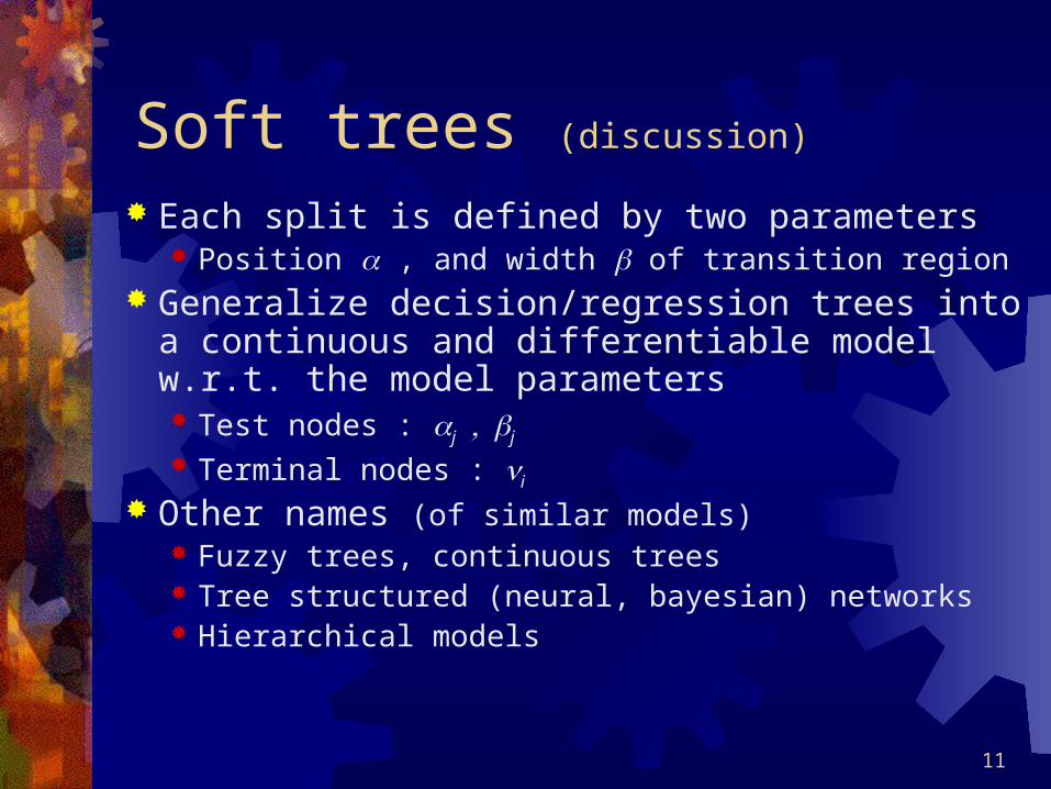
Soft trees (discussion)
Each split is defined by two parameters Position , and width of transition region
Generalize decision/regression trees into a continuous and differentiable model w.r.t. the model parameters Test nodes : jj Terminal nodes : i
Other names (of similar models) Fuzzy trees, continuous trees Tree structured (neural, bayesian) networks Hierarchical models

12
Soft trees (Motivations)
Improve performance (w.r.t. crisp trees) Use of a larger hypothesis space Reduced variance and bias Improved optimization (à la backprop)
Improve interpretability More « honest » model Reduced parameter variance Reduced complexity

13
D. Plan of the presentation
Bias/Variance tradeoff (in tree induction)
Main techniques to reduce variance
Why soft trees have lower variance
Techniques for learning soft trees

14
Concept of variance Learning sample is random Learned model is function of the sample
Model is also random variance Model predictions have variance Model structure / parameters have variance
Variance reduces accuracy and interpretability
Variance can be reduced by various ‘averaging or smoothing’ techniques

15
Theoretical explanation Bias, variance and residual error
Residual error Difference between output variable and the best possible model
(i.e. error of the Bayes model) Bias
Difference between the best possible model and the average model produced by algorithm
Variance Average variability of model around average model
Expected error2 : res2+bias2+var
NB: these notions depend on the ‘metric’ used for measuring error
16
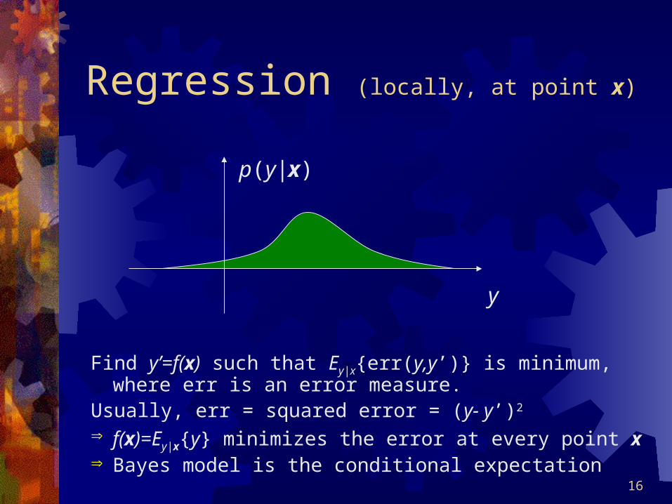
Regression (locally, at point x)
Find y’=f(x) such that Ey|x{err(y,y’)} is minimum, where err is an error measure.
Usually, err = squared error = (y- y’)2
f(x)=Ey|x{y} minimizes the error at every point x Bayes model is the conditional expectation
y
p(y|x)

17
Learning algorithm (1)
Usually, p(y|x) is unknown Use LS = ((x1,y1),…,(xN,yN)), and a learning
algorithm to choose hypothesis in ŷLS(x)=f(LS,x)
At each input point x, the prediction ŷLS(x) is a random variable
Distribution of ŷLS(x) depends on sample size N and on the learning algorithm used

18
Learning algorithm (2)
Since LS is randomly drawn, estimation ŷ(x) is a random variable
ŷ
pLS (ŷ(x))

19
Good learning algorithm
A good learning algorithm should minimize the average (generalization) error over all learning sets
In regression, the usual error is the mean squared error. So we want to minimize (at each point x)
Err(x)=ELS{Ey|x{(y-ŷLS(x))2}}
There exists a useful additive decomposition of this error into three (positive) terms
20
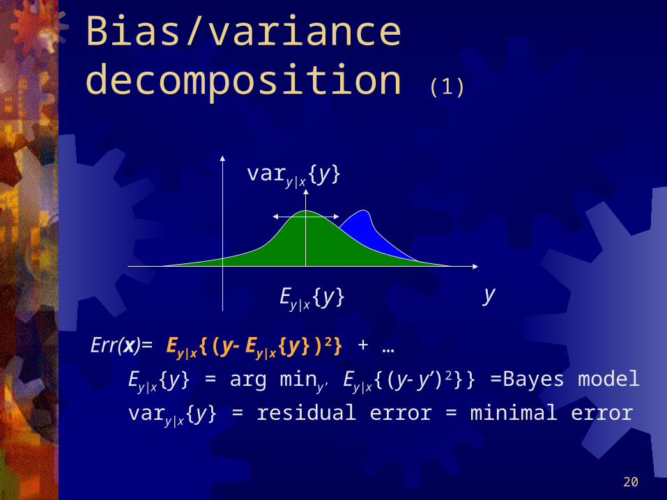
Bias/variance decomposition (1)
Err(x)= Ey|x{(y- Ey|x{y})2} + …
Ey|x{y} = arg miny’ Ey|x{(y- y’)2}} =Bayes model
vary|x{y} = residual error = minimal error
y
vary|x{y}
Ey|x{y}

21
Bias/variance decomposition (2)
Err(x) = vary|x{y} + (Ey|x{y}-ELS{ŷ(x)})2 + …
ELS{ŷ(x)} = average model (w.r.t. LS)
bias2(x) = error between Bayes and average model
ŷEy|x{y} ELS{ŷ(x)}
bias2(x)
22
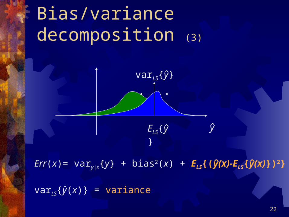
Bias/variance decomposition (3)
Err(x)= vary|x{y} + bias2(x) + ELS{(ŷ(x)-ELS{ŷ(x)})2}
varLS{ŷ(x)} = variance
ŷ
varLS{ŷ}
ELS{ŷ}

23
Bias/variance decomposition (4)
Local error decomposition Err(x) = vary|x{y} + bias2(x) + varLS{ŷ(x)}
Global error decomposition (take average w.r.t. p(x))EX{Err(x)} = EX{vary|x{y}} + EX{bias2(x)} + EX{varLS{ŷ(x)}}
ŷEy|x{y} ELS{ŷ(x)}
bias2(x)
vary|x{y} varLS{ŷ(x)}

24
Illustration (1)
Problem definition: One input x, uniform random variable in [0,1] y=h(x)+ε where εN(0,1)
h(x)=Ey|x{y}
x

25
Illustration (2)
Small variance, high bias method
ELS{ŷ(x)}

26
Illustration (3)
Small bias, high variance method
ELS{ŷ(x)}

27
Illustration (Methods comparison)
Artificial problem with 10 inputs, all uniform random variables in [0,1]
The true function depends only on 5 inputs:
y(x)=10.sin(π.x1.x2)+20.(x3-0.5)2+10.x4+5.x5+ε,
where ε is a N(0,1) random variable
Experimentation: ELS average over 50 learning sets of size 500 Ex,y average over 2000 cases Estimate variance and bias (+ residual error)
28
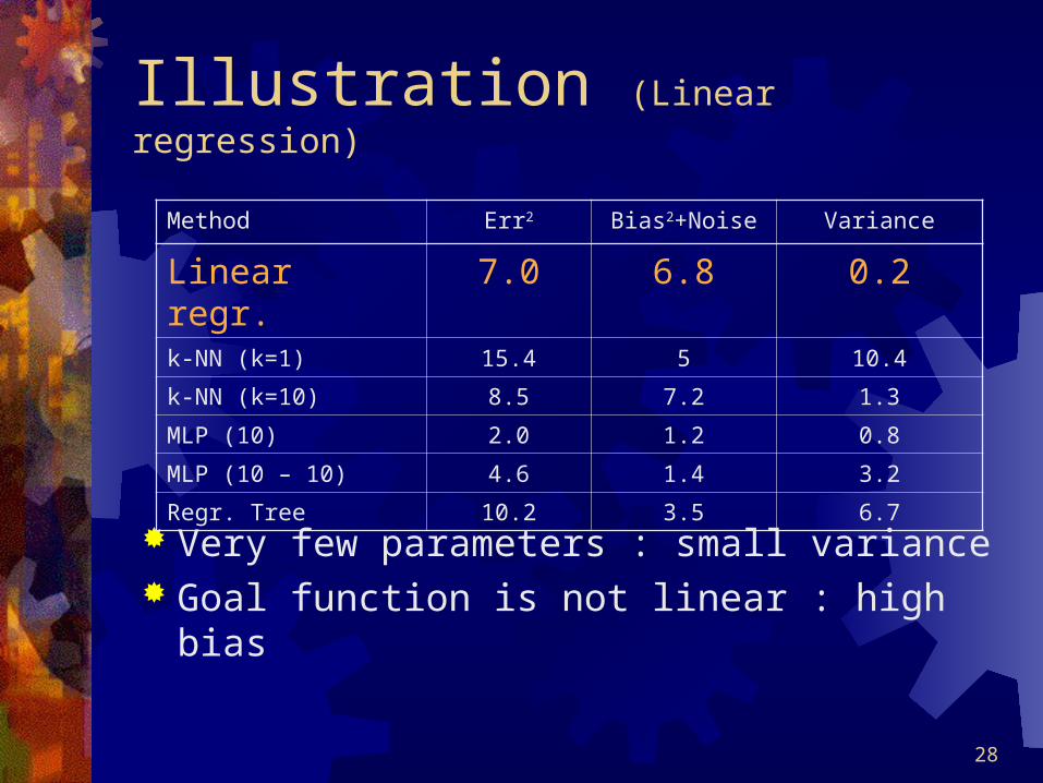
Illustration (Linear regression)
Very few parameters : small variance Goal function is not linear : high bias
Method Err2 Bias2+Noise Variance
Linear regr. 7.0 6.8 0.2k-NN (k=1) 15.4 5 10.4
k-NN (k=10) 8.5 7.2 1.3
MLP (10) 2.0 1.2 0.8
MLP (10 – 10) 4.6 1.4 3.2
Regr. Tree 10.2 3.5 6.7

29
Illustration (k-Nearest Neighbors)
Small k : high variance and moderate bias High k : smaller variance but higher bias
Method Err2 Bias2+Noise Variance
Linear regr. 7.0 6.8 0.2
k-NN (k=1) 15.4 5 10.4
k-NN (k=10) 8.5 7.2 1.3MLP (10) 2.0 1.2 0.8
MLP (10 – 10) 4.6 1.4 3.2
Regr. Tree 10.2 3.5 6.7
30
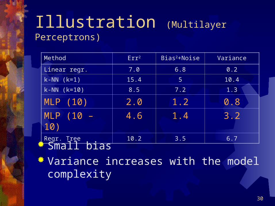
Illustration (Multilayer Perceptrons)
Small bias Variance increases with the model complexity
Method Err2 Bias2+Noise Variance
Linear regr. 7.0 6.8 0.2
k-NN (k=1) 15.4 5 10.4
k-NN (k=10) 8.5 7.2 1.3
MLP (10) 2.0 1.2 0.8
MLP (10 – 10) 4.6 1.4 3.2Regr. Tree 10.2 3.5 6.7

31
Illustration (Regression trees)
Small bias, a (complex enough) tree can approximate any non linear function
High variance (see later)
Method Err2 Bias2+Noise Variance
Linear regr. 7.0 6.8 0.2
k-NN (k=1) 15.4 5 10.4
k-NN (k=10) 8.5 7.2 1.3
MLP (10) 2.0 1.2 0.8
MLP (10 – 10) 4.6 1.4 3.2
Regr. Tree 10.2 3.5 6.7

32
Variance reduction techniques In the context of a given method:
Adapt the learning algorithm to find the best trade-off between bias and variance.
Not a panacea but the least we can do. Example: pruning, weight decay.
Wrapper techniques: Change the bias/variance trade-off. Universal but destroys some features of the initial
method. Example: bagging.

33
Variance reduction: 1 model (1)
General idea: reduce the ability of the learning algorithm to over-fit the LS Pruning
reduces the model complexity explicitly Early stopping
reduces the amount of search Regularization
reduce the size of hypothesis space

34
Variance reduction: 1 model (2)
Bias2 error on the learning set, E error on an independent test set
Selection of the optimal level of tuning a priori (not optimal) by cross-validation (less efficient)
E=bias2+var
bias2
var
Fitting
Optimal fitting
35
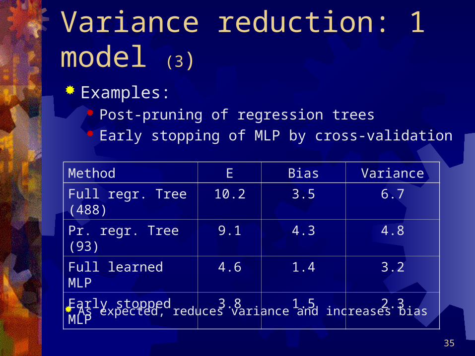
Variance reduction: 1 model (3)
As expected, reduces variance and increases bias
Examples: Post-pruning of regression trees Early stopping of MLP by cross-validation
Method E Bias Variance
Full regr. Tree (488) 10.2 3.5 6.7
Pr. regr. Tree (93) 9.1 4.3 4.8
Full learned MLP 4.6 1.4 3.2
Early stopped MLP 3.8 1.5 2.3
36
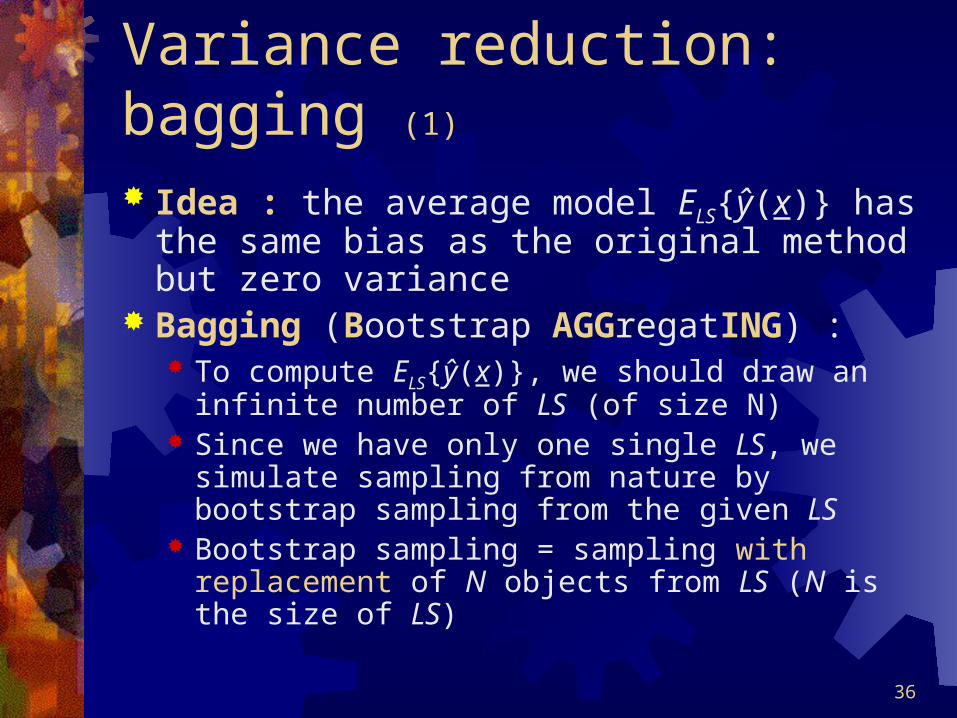
Variance reduction: bagging (1)
Idea : the average model ELS{ŷ(x)} has the same bias as the original method but zero variance
Bagging (Bootstrap AGGregatING) : To compute ELS{ŷ(x)}, we should draw an infinite
number of LS (of size N) Since we have only one single LS, we simulate
sampling from nature by bootstrap sampling from the given LS
Bootstrap sampling = sampling with replacement of N objects from LS (N is the size of LS)

37
Variance reduction: bagging (2)
LS
LS1 LS2 LSk
ŷ1(x) ŷ2(x) ŷk(x)
ŷ(x) = 1/k.(ŷ1(x)+ŷ2(x)+…+ŷk(x))
x

38
Variance reduction: bagging (3)
Application to regression trees
Strong variance reduction without increasing bias (although the model is much more complex than a single tree)
Method E Bias Variance
3 Test regr. Tree 14.8 11.1 3.7
Bagged 11.7 10.7 1.0
Full regr. Tree 10.2 3.5 6.7
Bagged 5.3 3.8 1.5
39
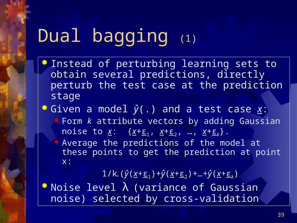
Dual bagging (1)
Instead of perturbing learning sets to obtain several predictions, directly perturb the test case at the prediction stage
Given a model ŷ(.) and a test case x: Form k attribute vectors by adding Gaussian noise
to x: {x+ε1, x+ε2, …, x+εk}. Average the predictions of the model at these
points to get the prediction at point x:
1/k.(ŷ(x+ε1)+ŷ(x+ε2)+…+ŷ(x+εk)
Noise level λ (variance of Gaussian noise) selected by cross-validation

40
Dual bagging (2)
With regression trees:
Smooth the function ŷ(.). Too much noise increases bias
there is a (new) trade-off between bias and variance
Noise level E Bias Variance
0.0 10.2 3.5 6.7
0.2 6.3 3.5 2.8
0.5 5.3 4.4 0.9
2.0 13.3 13.1 0.2

41
Dual bagging (classification trees)
λ = 0 error =3.7 %
λ = 1.5 error =4.6 %
λ = 0.3 error =1.4 %

42
Variance in tree induction Tree induction is among the ML methods of highest variance
(together with 1-NN) Main reason
Generalization is local Depends on small parts of the learning set
Sources of variance: Discretization of numerical attributes (60 %)
The selected thresholds have a high variance Structure choice (10 %)
Sometimes, attribute scores are very close Estimation at leaf nodes (30 %)
Because of the recursive partitioning, prediction at leaf nodes is based on very small samples of objects
Consequences: Questionable interpretability and higher error rates

43
Threshold variance (1)
Test on numerical attributes : [a(o)<ath]
Discretization: find ath which minimizes score Classification: maximize information Regression: minimize residual variance
Score
ath
a(o)

44
Threshold variance (2)
E m p iric a l o p tim a l th re sh o ld d is trib u tion
N =10 0
S co re c u rv es
800. 900. 1000. 1100. 1200.-- - Thres hold - --
0.0
0.1
0.2
0.3
0.4
Sc ore/N b o f c as es

45
Threshold variance (3)
E m p irica l o p tim a l th re sh o ld d is trib u tion
N =1 00 0
S co re cu rve s
800. 900. 1000. 1100. 1200.- - - Thres hold -- -
0.0
5.e-2
0.1
0.15
0.2
0.25
S c ore/N b of c as es

46
Tree variance DT/RT are among the machine learning
methods which present the highest variance
Method E Bias Variance
RT, no test 25.5 25.4 0.1
RT, 1 test 19.0 17.7 1.3
RT, 3 tests 14.8 11.1 3.7
RT, full (250 tests) 10.2 3.5 6.7

47
DT variance reduction Pruning:
Necessary to select the right complexity Decreases variance but increases bias : small effect on accuracy
Threshold stabilization: Smoothing of score curves, bootstrap sampling… Reduces parameter variance but has only a slight effect on
accuracy and prediction variance Bagging:
Very efficient at reducing variance But jeopardizes interpretability of trees and computational efficiency
Dual bagging: In terms of variance reduction, similar to bagging Much faster and can be simulated by soft trees
Fuzzy tree induction Build soft trees in a full fledged approach

48
Dual tree bagging = Soft treesReformulation of dual bagging as an
explicit soft tree propagation algorithmAlgorithms
Forward-backward propagation in soft trees
Softening of thresholds during learning stage
Some results

49
Dual bagging = soft thresholds x+ε<xth sometimes left, sometimes right Multiple ‘crisp’ propagations can be ‘replaced’
by one ‘soft’ propagation E.g. if ε has uniform pdf in [ath- /2,ath+ /2]
then probability of right propagation is as follows
ath
TSleft TSright

50
Forward-backward algorithm Top-down propagation of probability
P(L3|x) = P(Test1|x)P(Root|x)
Root
N1 L3
L2L1
P(Root|x)=1
Test1P(N1|x) = P(Test1|x) P(Root|x)
Test2
P(L1|x) = P(Test2|x)P(N1|x)
P(L2|x) = P(Test2|x)P(N1|x)
Bottom-up aggregation of predictions

51
Learning of values
Use of an independent ‘validation’ set and bisection search
One single value can be learned very efficiently (amounts to 10 full tests of a DT/RT on the validation set)
Combination of several values can also be learned with the risk of overfitting (see fuzzy tree induction, in what follows)

52
Some results with dual bagging
0
5
10
15
20
25Pe % DT
DT + Dual BaggBaggingBagging + Dual
53
Fuzzy tree inductionGeneral ideasLearning Algorithm
Growing Refitting Pruning Backfitting

54
General IdeasObviously, soft trees have much lower
variance than crisp trees In the « Dual Bagging » approach,
attribute selection is carried out in a cloassical way, then tests are softened in a post-processing stage
Might be more effective to combine the two methods
Fuzzy tree induction

55
Soft trees Samples are handled as fuzzy subsets
Each observation belongs to such a FS with a certain membership degree
SCORE measure is modified Objects are weighted by their membership degree
Output y Denotes the membership degree to a class
Goal of Fuzzy tree induction Provide a smooth model of ‘y’ as a function of the
input variables

56
Fuzzy discretization Same as fuzzification Carried out locally, at the tree growing stage
At each test node On the basis of local fuzzy sub-training set
Select attribute, together with discriminator so as to maximize local SCORE
Split in soft way and proceed recursively
Criteria for SCORE Minimal residual variance Maximal (fuzzy) information quantity Etc

57
Attaching labels to leaves Basically, for each terminal node, we need to
determine a local estimate ŷi of y During intermediate steps
Use average of ‘y’ in local sub-learning set Direct computation
Refitting of the labels Once the full tree has been grown and at each step of
pruning Determine all values simultaneously To minimize Square Error Amounts to a linear least squares problem Direct solution
58
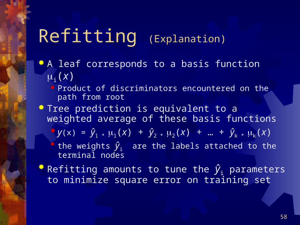
Refitting (Explanation)
A leaf corresponds to a basis function i(x) Product of discriminators encountered on the path
from root Tree prediction is equivalent to a weighted
average of these basis functions y(x) = ŷ1 * 1(x) + ŷ2 * 2(x) + … + ŷk * k(x) the weights ŷi are the labels attached to the
terminal nodes
Refitting amounts to tune the ŷi parameters to minimize square error on training set
59
Tree growing and pruningGrow treeRefit leaf labelsPrune tree, while refitting at each stage
leaf labelsTest sequence of pruned trees on
validation setSelect best pruning level
60
Backfitting (1)
After growing and pruning, the fuzzy tree structure has been determined
Leaf labels are globally optimal, but not the parameters of the discriminators (tuned locally)
Resulting model has 2 parameters per test node, and 1 parameter per terminal node
The output (and hence Mean square error) of the fuzzy tree is a smooth function of these parameters
The parameters can be optimized, by using a standard LSE technique, e.g. Levenberg-Marquardt

61
Backfitting (2)
How to compute the derivatives needed by nonlinear optimization technique Use a modified version of backpropagation to compute
derivates with respect to parameters Yields an efficient algorithm (linear in the size of the tree)
Backfitting starts from tree produced after growing and pruning Already a good approximation of a local optimum Only a small number of iterations are necessary to backfit
Backfitting may also lead to overfitting…
62
Summary and conclusions Variance is the problem number one in
decision/regression tree induction It is possible to reduce variance significantly
Bagging and/or tree softening Soft trees have the advantage of preserving interpretability
and computational efficiency Two approaches have been presented to get soft trees
Dual bagging Generic approach Fast and simple Best approach for very large databases
Fuzzy tree induction Similar to ANN type of model, but (more) interpretable Best approach for small learning sets (probably)

63
Some references for further reading Variance evaluation/reduction, bagging
Contact : Pierre GEURTS (PhD student) [email protected]
Papers Discretization of continuous attributes for supervised learning -
Variance evaluation and variance reduction. (Invited) L. Wehenkel. Proc. of IFSA'97, International Fuzzy Systems Association World Congress, Prague, June 1997, pp. 381--388.
Investigation and Reduction of Discretization Variance in Decision Tree Induction. Pierre GEURTS and Louis WEHENKEL, Proc. of ECML’2000
Some Enhancements of Decision Tree Bagging. Pierre GEURTS, Proc. of PKDD’2000
Dual Perturb and Combine Algorithm. Pierre GEURTS, Proc. of AI and Statistics 2001.

64
See also www.montefiore.ulg.ac.be/services/stochastic/
Fuzzy/soft tree induction Contact : Cristina OLARU (PhD student)
[email protected] Papers
Automatic induction of fuzzy decision trees and its application to power system security assessment. X. Boyen, L. Wehenkel, Int. Journal on Fuzzy Sets and Systems, Vol. 102, No 1, pp. 3-19, 1999.
On neurofuzzy and fuzzy decision trees approaches. C. Olaru, L. Wehenkel. (Invited) Proc. of IPMU'98, 7th Int. Congr. on Information Processing and Management of Uncertainty in Knowledge based Systems, 1998.