1 regionknn: a scalable hybrid collaborative filtering algorithm for personalized web service...
TRANSCRIPT

1
RegionKNN: A Scalable Hybrid Collaborative Filtering Algorithm for Personalized Web
Service Recommendation
Xi Chen, Xudong Liu, Zicheng Huang, and Hailong Sun
School of Computer Science and EngineeringBeihang University
Beijing, China

2
Outline
• Introduction
• Motivation
• RegionKNN Algorithm
• Experiments
• Conclusion and Future Work

3
1. Introduction

4
Introduction
• Current situation– More than 25,000 public available services (seekda.com)– About 200,000 related documents
• Goal of service recommendation– Optimal QoS– User preference
• Current method: Collaborative Filtering (CF) – predict and recommend the potential favorite items for a
particular user by using rating data collected from similar users.
• If Alice and Bob both like X and Alice likes Y then Bob is more likely to like Y
• Problems– Characteristics of QoS are neglected– Online performance need to be improved

5
2. Motivation

6
A Motivating Scenario
Some QoS properties (e.g. availability, response time) highly correlate to users’ physical locations.
EmailFiltering
WS
EmailFiltering
WS

7
3. RegionKNN Algorithm

8
What’s RegionKNN• Hybrid CF Algorithm
– recommend web services with optimal QoS to the active user with consideration of the region factor
• Two phases of RegionKNN– Region model building (offline)
• Region-sensitive services identification
• Region aggregation
– Service recommendation (online) (modified KNN) • Neighbor selection
• QoS Prediction
I take response time/round trip time (RTT) as an example to describe our algorithm

9
3.1 Region model

10
Region Model• Region
– a group of users who are closely located with each other and have similar RTT values
u5
u19 u2u22,u8
u1, u3
Service A Service A
Service B Service B
Service X Service X

11
Input Dataset
• User-Service RTT Matrix: m services, n users
• The set of non-zero RTTs of service s {R1(s), R2(s),…, Rk(s)} collected from all users is a sample from population R.
s1 s2 … sm
u1 0 245 … 20078
u2 2023 342 … 539
… … … … …
un 0 3040 … 498
RTT is much longer than
others

12
Region-sensitive Services Identification
• To estimate the mean μ and the standard deviation σ of R, we use:
))((ˆ sRmedian ii
))((4862.1ˆ sRMAD ii
Median: the numeric value separating the higher half of a sample from the lower half. e.g. {120, 128, 200, 250, 258, 2000, 3500} median = 250
MAD: the Median of the Absolute Deviations from the sample's median. e.g. {120, 128, 200, 250, 258, 2000, 3500} {8, 50, 122, 130, 1750, 2250} MAD = 130

13
• Region-Sensitive Service– Let R = {R1(s), R2(s),…, Rk(s)} be the set of RTTs of service s
provided by users from all regions. Service s is a sensitive service to region M iff
))()ˆ3ˆ)((()( MjregionsRRsR jj
{120, 128, 200, 250, 258, 2000, 3500}
u1 u3 u5 u19 u2 u22 u8
u5
u19 u2
u22
u8u1, u3
Service A
Service A
Region-sensitive services Identification

14
Definition
• Region Sensitivity
• Sensitive Region– Region M is a sensitive region iff regSen >λ.
• Region center – the median vector of all the RTT vectors provided by
users in a region
||
||)(
services
ervicessensitivesMregSen

15
Region Aggregation
• Why?– Users only provide limited number of QoS values, the
sparse dataset always leads to poor recommendation.
• How?– It treats users with similar IP addresses as a region at
the outset – In each iteration, the two most similar and non-sensitive
regions are selected and aggregated, if their similarity exceeds threshold μ.
– It executes at most N-1 steps (N is the number of regions at the outset), in case that all regions are non-sensitive, extremely correlates to each other and finally aggregates into one region.

16
Region Similarity• The similarity between region M and N is measured by
the similarity of the two centers. • Similarity by Pearson Correlation Coefficient (PCC)
)()(
2
)()(
2
)()(
))(())((
))(())((
),(
mSnSsnn
mSnSsmm
nnmSnSs
mm
RsRRsR
RsRRsR
nmSim
s1 s2 s3 s4 s5
cm 1 2 5 0 0
cn 0 0 5 1 3
By PCC, the similarity is of the two regions is 1

17
Region Similarity
• PCC often overestimates the similarity when the two regions have few co-invoked services. To adjust it, we use:
),(|)()(|
|)()(|),( nmSim
nSmS
nSmSnmmSi
s1 s2 s3 s4 s5
cm 1 2 5 0 0
cn 0 0 5 1 3
By adjustment, the similarity of the two regions is 0.2

18
3.2 Service Recommendation

19
Neighbor Selection
• Neighbors: users with similar QoS experiences• Advantages of region-based neighbor selection
– Do not need to search the entire dataset, thousands of users are clustered into a certain number of regions
– The feature of the group of users in a region is represented by the region center

20
QoS Prediction
• To calculate the RTT prediction for the active user u and service si
• Get the active user’s IP address and find the region the user belongs to. If no appropriate region is found, the active user will be treated as a member of a new region.
• Identify whether service si is sensitive to the specific region. If it is region-sensitive, then the prediction is generated from the region center:
)(ˆ iu sR
)()(ˆ icenteriu sRsR

21
QoS Prediction (cont.)
• Otherwise, use adjusted PCC to compute the similarity between the active user and each region center that has evaluated service si, and find up to k most similar centers {c1, c2,…, ck}.
• If the active user’s region center has the RTT value of si, i.e. , the prediction is computed using the equation:
0)( icenter sR
k
j j
k
j jcic
icenteriucumSi
cumSiRsRsRsR jj
1
1
),(
),())(()()(ˆ
22
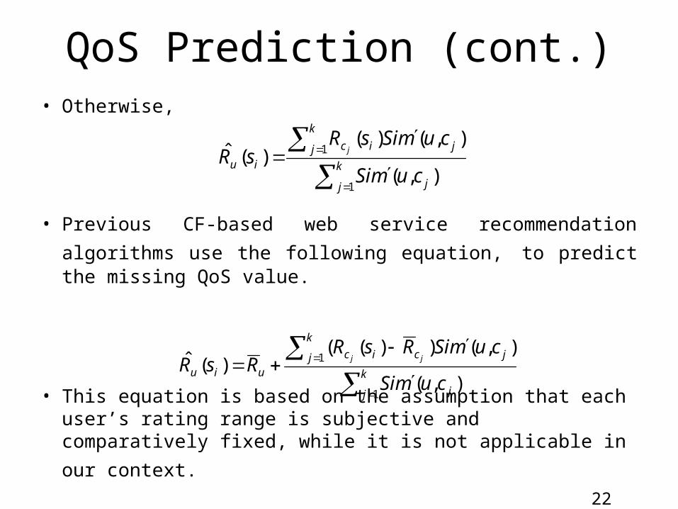
QoS Prediction (cont.)• Otherwise,
• Previous CF-based web service recommendation
algorithms use the following equation, to predict the missing QoS value.
• This equation is based on the assumption that each user’s rating range is subjective and comparatively fixed, while it
is not applicable in our context.
k
j j
k
j jic
iucumSi
cumSisRsR j
1
1
),(
),()()(ˆ
k
j j
k
j jcic
uiucumSi
cumSiRsRRsR jj
1
1
),(
),())(()(ˆ

23
Time complexity
• Model building (offline)– The time complexity of region aggregation algorithm
is O(N2logN), and N is the number of regions at the outset.
• QoS prediction (online)– Let l be the number of regions, m the number of web
services, and n the number of users. In the online part, O(l) similarity weight calculations are needed, each of which takes O(m) time. Therefore, the online time-complexity is O(lm)≈O(m). Previous user-based CF algorithm has O(mn) online time complexity.

24
4. Experiments

25
Experiments
• Dataset– a subset of WSRec with 300,000 RTT records– 3000 users – 100 services
• Evaluation Metric
– Ru(s) denotes the actual RTT of web service s given by user u
– denotes the predicted one– L denotes the number of tested services
L
sRsR
MAE suuu
,
|)(ˆ)(|
)(ˆ sRu
Dataset: http://www.wsdream.net

26
MAE Performance

27
Impact of λ and μ

28
Impact of neighborhood size K

29
Impact of Data Sparsity

30
5.Conclustion and Future Work

31
Conclusion and Future Work
• Conclusion– a new region model for clustering users and
identifying region-sensitive web services– a hybrid model-based and memory-based CF
algorithm for web service recommendation, which significantly improves the recommendation accuracy
– We demonstrate RegionKNN’s scalability advantage over traditional CF algorithms via time-complexity analysis
• Future Work– Investigation of more QoS properties and their
variation with time – Internal relations between QoS properties

32