1

Regression Models and Loss Reserving

Regression Models and Loss Reserving

Leigh J. Halliwell, FCAS, MAAA

EPIC Consulting, LLC

lhalliwell@ask-epic.com

Casualty Loss Reserve Seminar

Las Vegas, NV

September 14, 2004

Leigh J. Halliwell, FCAS, MAAA

EPIC Consulting, LLC

lhalliwell@ask-epic.com

Casualty Loss Reserve Seminar

Las Vegas, NV

September 14, 2004

2

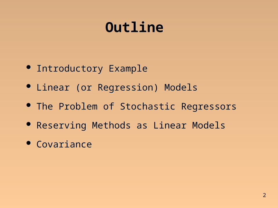
OutlineOutline

Introductory Example

Linear (or Regression) Models

The Problem of Stochastic Regressors

Reserving Methods as Linear Models

Covariance

Introductory Example

Linear (or Regression) Models

The Problem of Stochastic Regressors

Reserving Methods as Linear Models

Covariance

3

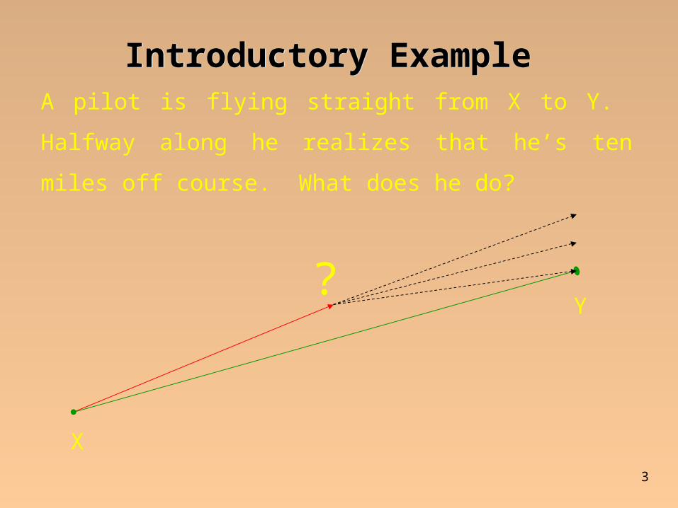
Introductory ExampleIntroductory Example

A pilot is flying straight from X to Y. Halfway along he

realizes that he’s ten miles off course. What does he do?

X

Y?

4

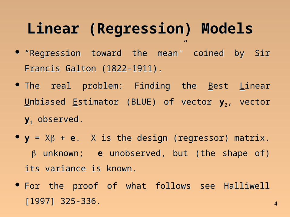
Linear (Regression) ModelsLinear (Regression) Models

“Regression toward the mean” coined by Sir Francis

Galton (1822-1911).

The real problem: Finding the Best Linear Unbiased

Estimator (BLUE) of vector y2, vector y1 observed.

y = X + e. X is the design (regressor) matrix.

unknown; e unobserved, but (the shape of) its variance

is known.

For the proof of what follows see Halliwell [1997] 325-

336.

“Regression toward the mean” coined by Sir Francis

Galton (1822-1911).

The real problem: Finding the Best Linear Unbiased

Estimator (BLUE) of vector y2, vector y1 observed.

y = X + e. X is the design (regressor) matrix.

unknown; e unobserved, but (the shape of) its variance

is known.

For the proof of what follows see Halliwell [1997] 325-

336.

5

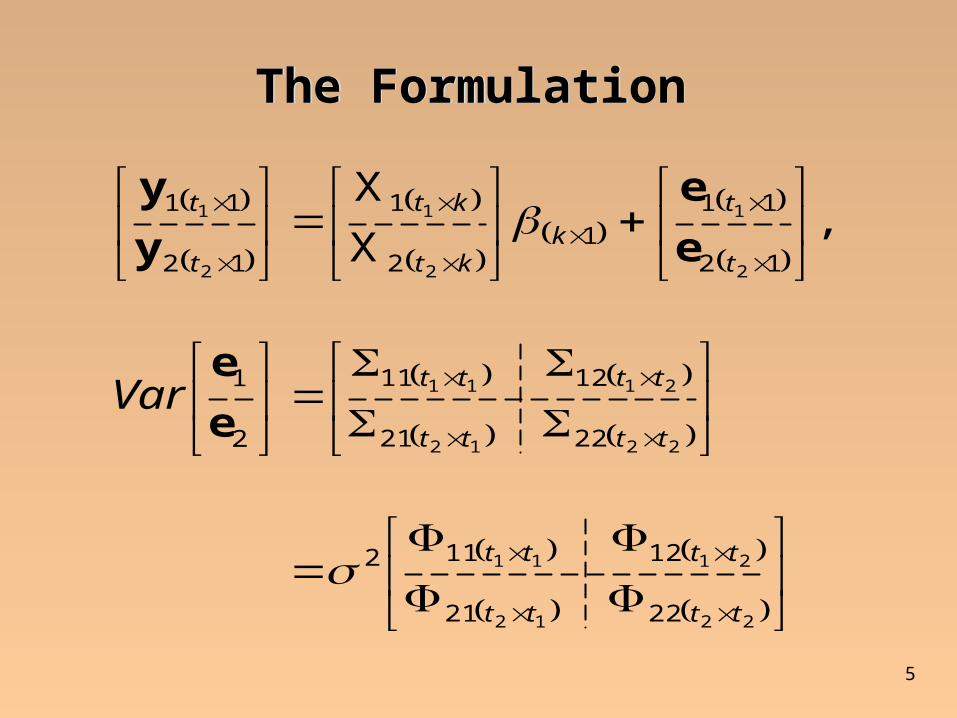
The FormulationThe Formulation

2212

2111

2212

2111

2

1

2

1

2

1

2221

12112

2221

1211

2

1

12

11

12

1

12

11,

X

X

tttt

tttt

tttt

tttt

t

t

kkt

kt

t

t

Var

e

e

e

e

y

y

6

Trend ExampleTrend Example

3353

35552

2

1

132

15112

132

151

I00I

,

8171615141312111

ee

ee

yy

Var

7

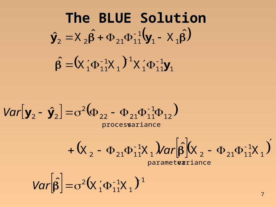
The BLUE SolutionThe BLUE Solution

1

11

1112

varianceparameter 1

1112121

111212

varianceprocess12

1112122

222

11

111

1

11

111

111

112122

XXˆ

XXˆXX

ˆ

XXXˆ

ˆXˆXˆ

Var

Var

Var yy

y

yy

8

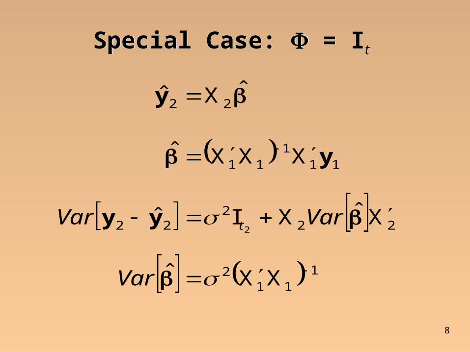
Special Case: = ItSpecial Case: = It

1

112

222

22

111

11

22

XXˆ

XˆXIˆ

XXXˆ

ˆXˆ

2

Var

VarVar tyy

y

y

9

Estimator of the Variance ScaleEstimator of the Variance Scale

kt

1

111

11112ˆXˆX

ˆ

yy

10

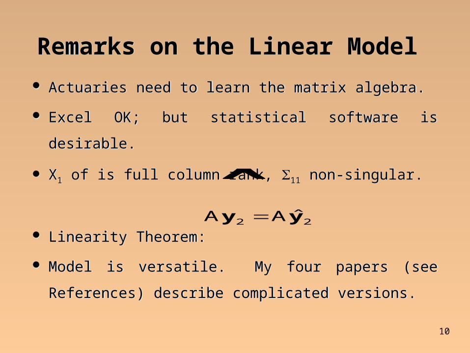
Remarks on the Linear ModelRemarks on the Linear Model

Actuaries need to learn the matrix algebra.

Excel OK; but statistical software is desirable.

X1 of is full column rank, 11 non-singular.

Linearity Theorem:

Model is versatile. My four papers (see References)

describe complicated versions.

Actuaries need to learn the matrix algebra.

Excel OK; but statistical software is desirable.

X1 of is full column rank, 11 non-singular.

Linearity Theorem:

Model is versatile. My four papers (see References)

describe complicated versions.

22 ˆAA

yy

11

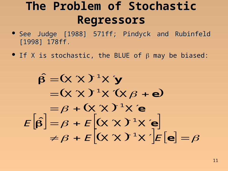
The Problem of Stochastic RegressorsThe Problem of Stochastic Regressors

See Judge [1988] 571ff; Pindyck and Rubinfeld [1998] 178ff.

If X is stochastic, the BLUE of may be biased:

See Judge [1988] 571ff; Pindyck and Rubinfeld [1998] 178ff.

If X is stochastic, the BLUE of may be biased:

e

e

e

e

y

EE

EE

XXX

XXXˆ

XXX

XXXX

XXXˆ

1

1

1

1

1

12

The Clue: Regression toward the MeanThe Clue: Regression toward the MeanTo intercept or not to intercept?To intercept or not to intercept?

0

2,000

4,000

6,000

8,000

10,000

12,000

14,000

16,000

18,000

0 1,000 2,000 3,000 4,000 5,000 6,000

Loss @12

Loss

@24

13

What to do?What to do?

Ignore it.

Add an intercept.

Barnett and Zehnwirth [1998] 10-13, notice that the

significance of the slope suffers. The lagged loss may

not be a good predictor.

Intercept should be proportional to exposure.

Explain the torsion. Leads to a better model?

Ignore it.

Add an intercept.

Barnett and Zehnwirth [1998] 10-13, notice that the

significance of the slope suffers. The lagged loss may

not be a good predictor.

Intercept should be proportional to exposure.

Explain the torsion. Leads to a better model?

14

Galton’s ExplanationGalton’s Explanation

Children's heights regress toward the mean. Tall fathers tend to have sons shorter than themselves. Short fathers tend to have sons taller than themselves.

Height = “genetic height” + environmental error A son inherits his father’s genetic height:

Son’s height = father’s genetic height + error.

A father’s height proxies for his genetic height. A tall father probably is less tall genetically. A short father probably is less short genetically.

Excellent discussion in Bulmer [1979] 218-221.

Children's heights regress toward the mean. Tall fathers tend to have sons shorter than themselves. Short fathers tend to have sons taller than themselves.

Height = “genetic height” + environmental error A son inherits his father’s genetic height:

Son’s height = father’s genetic height + error.

A father’s height proxies for his genetic height. A tall father probably is less tall genetically. A short father probably is less short genetically.

Excellent discussion in Bulmer [1979] 218-221.

15

The Lesson for ActuariesThe Lesson for Actuaries Loss is a function of exposure. Losses in the design matrix, i.e., stochastic

regressors (SR), are probably just proxies for exposures. Zero loss proxies zero exposure.

The more a loss varies, the poorer it proxies. The torsion of the regression line is the clue. Reserving actuaries tend to ignore exposures –

some even glad not to have to “bother” with them! SR may not even be significant. Covariance is an alternative to SR (see later). Stochastic regressors are nothing but trouble!!

Loss is a function of exposure. Losses in the design matrix, i.e., stochastic

regressors (SR), are probably just proxies for exposures. Zero loss proxies zero exposure.

The more a loss varies, the poorer it proxies. The torsion of the regression line is the clue. Reserving actuaries tend to ignore exposures –

some even glad not to have to “bother” with them! SR may not even be significant. Covariance is an alternative to SR (see later). Stochastic regressors are nothing but trouble!!

16

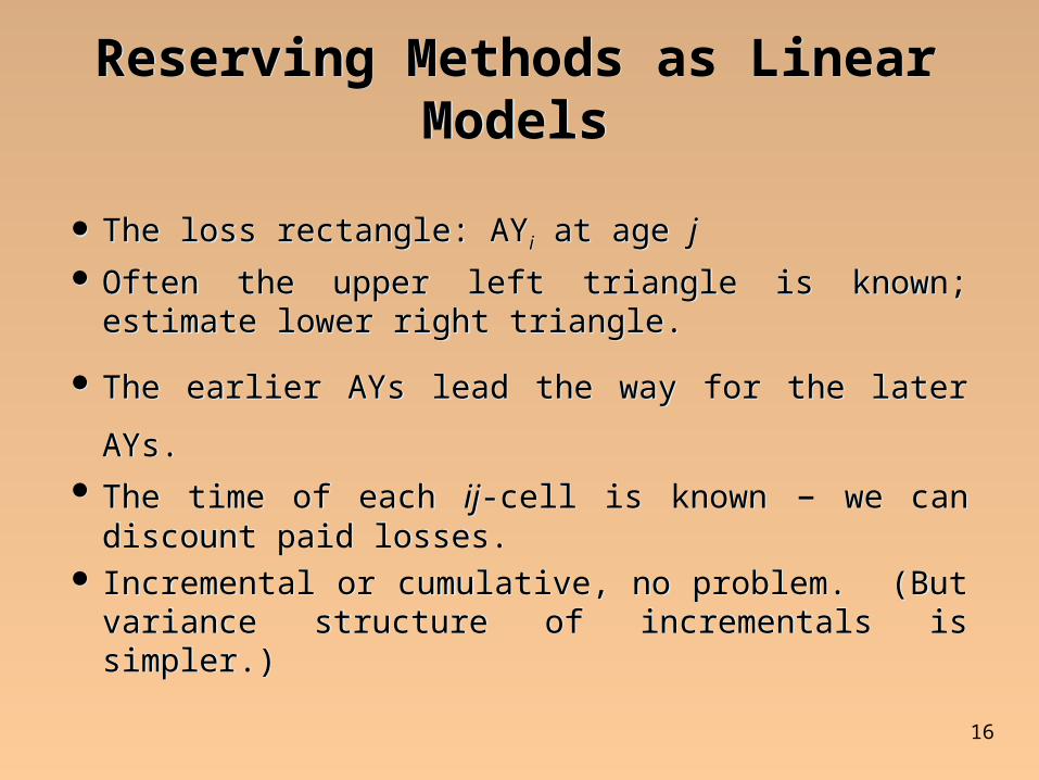
Reserving Methods as Linear ModelsReserving Methods as Linear Models

The loss rectangle: AYi at age j Often the upper left triangle is known; estimate

lower right triangle.

The earlier AYs lead the way for the later AYs. The time of each ij-cell is known – we can

discount paid losses. Incremental or cumulative, no problem. (But

variance structure of incrementals is simpler.)

The loss rectangle: AYi at age j Often the upper left triangle is known; estimate

lower right triangle.

The earlier AYs lead the way for the later AYs. The time of each ij-cell is known – we can

discount paid losses. Incremental or cumulative, no problem. (But

variance structure of incrementals is simpler.)

17

The Basic Linear ModelThe Basic Linear Model

yij incremental loss of ij-cell

aij adjustments (if needed, otherwise = 1)

xi exposure (relativity) of AYi

fj incremental factor for age j (sum constrained)

r pure premium

eij error term of ij-cell

yij incremental loss of ij-cell

aij adjustments (if needed, otherwise = 1)

xi exposure (relativity) of AYi

fj incremental factor for age j (sum constrained)

r pure premium

eij error term of ij-cell

1 j

jijjiijij frfxa ey

18

Familiar Reserving MethodsFamiliar Reserving Methods

Additive

Bühlmann-StanardFerguson-rBornhuette1

LadderChain X

ijjiij

ijjiij

ijjiij

ijijij

rfxrfx

rfxrxf

eyeyeyey

eY

BF estimates zero parameters. BF, SB, and Additive constitute a progression. The four other permutations are less interesting. No stochastic regressors

BF estimates zero parameters. BF, SB, and Additive constitute a progression. The four other permutations are less interesting. No stochastic regressors

19

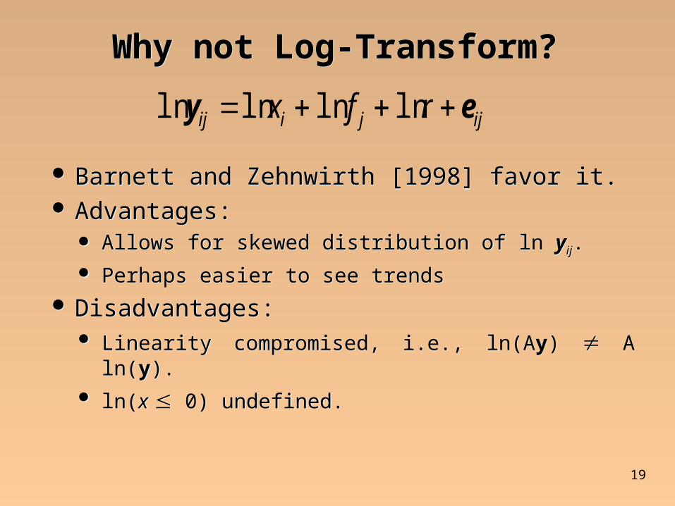
Why not Log-Transform?Why not Log-Transform?

Barnett and Zehnwirth [1998] favor it. Advantages:

Allows for skewed distribution of ln yij. Perhaps easier to see trends

Disadvantages: Linearity compromised, i.e., ln(Ay) A ln(y). ln(x 0) undefined.

Barnett and Zehnwirth [1998] favor it. Advantages:

Allows for skewed distribution of ln yij. Perhaps easier to see trends

Disadvantages: Linearity compromised, i.e., ln(Ay) A ln(y). ln(x 0) undefined.

ijjiij rfx ey lnlnlnln

20

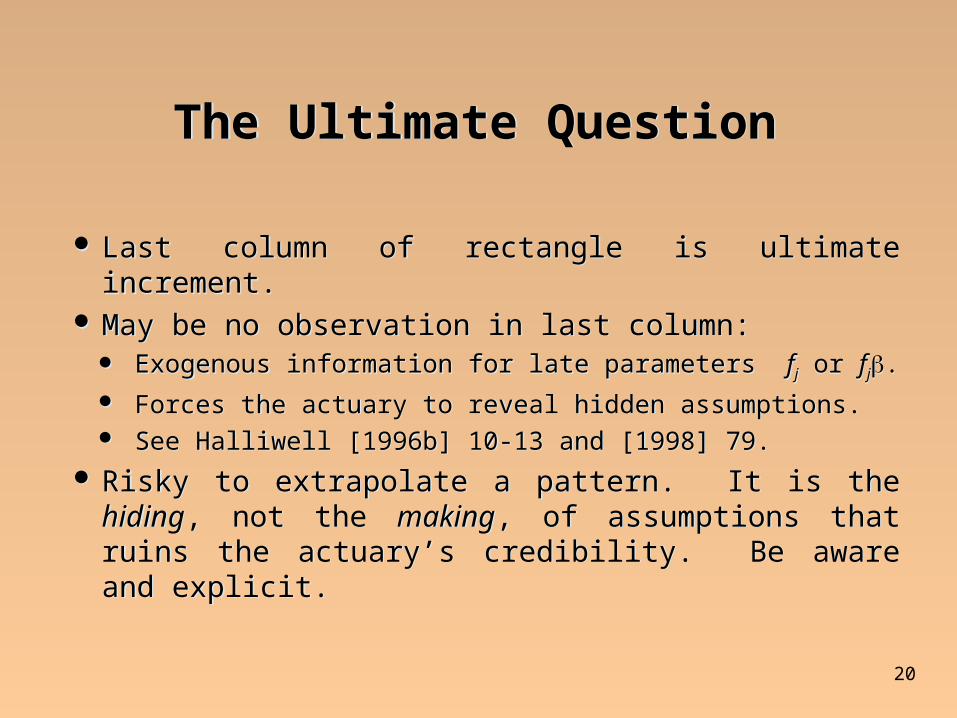
The Ultimate QuestionThe Ultimate Question

Last column of rectangle is ultimate increment. May be no observation in last column:

Exogenous information for late parameters fj or fj. Forces the actuary to reveal hidden assumptions. See Halliwell [1996b] 10-13 and [1998] 79.

Risky to extrapolate a pattern. It is the hiding, not the making, of assumptions that ruins the actuary’s credibility. Be aware and explicit.

Last column of rectangle is ultimate increment. May be no observation in last column:

Exogenous information for late parameters fj or fj. Forces the actuary to reveal hidden assumptions. See Halliwell [1996b] 10-13 and [1998] 79.

Risky to extrapolate a pattern. It is the hiding, not the making, of assumptions that ruins the actuary’s credibility. Be aware and explicit.

21

Linear TransformationsLinear Transformations

Results: and Interesting quantities are normally linear: AY totals and grand totals Present values

Powerful theorems (Halliwell [1997] 303f):

The present-value matrix is diagonal in the discount factors.

Results: and Interesting quantities are normally linear: AY totals and grand totals Present values

Powerful theorems (Halliwell [1997] 303f):

The present-value matrix is diagonal in the discount factors.

2y 22 yy Var

AˆAˆAA

ˆAˆA

2222

22

yyyy

yy

VarVar

EE

22

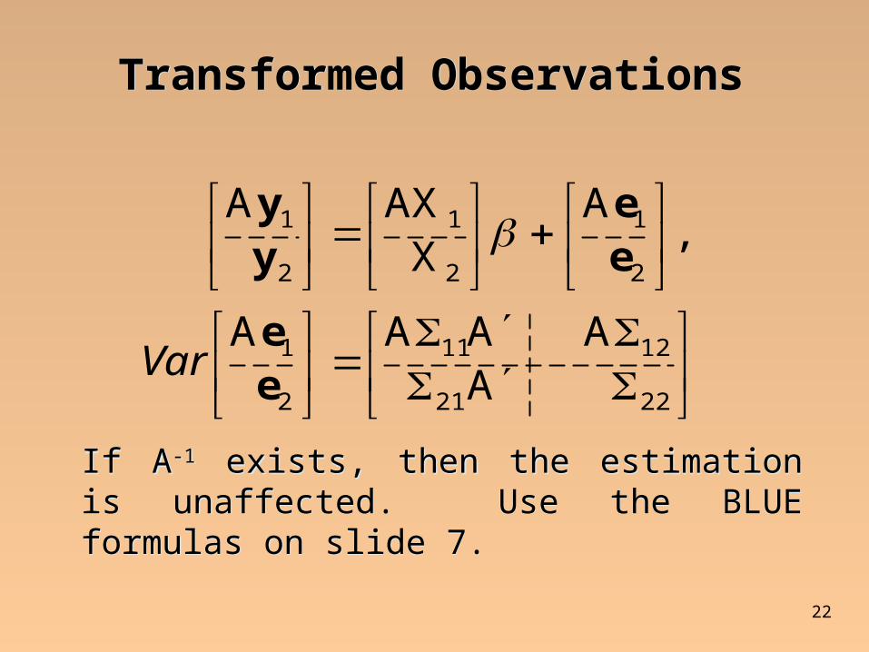
Transformed ObservationsTransformed Observations

2221

1211

2

1

2

1

2

1

2

1

AAAAA

,A

XAXA

ee

ee

yy

Var

If A-1 exists, then the estimation is unaffected. Use the BLUE formulas on slide 7.If A-1 exists, then the estimation is unaffected. Use the BLUE formulas on slide 7.

23

Example in ExcelExample in Excel

WC Example.lnk

24

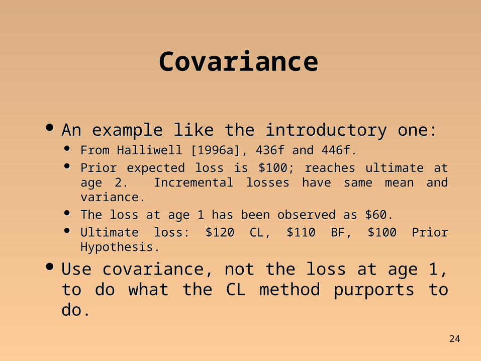
CovarianceCovariance

An example like the introductory one: From Halliwell [1996a], 436f and 446f. Prior expected loss is $100; reaches ultimate at age 2.

Incremental losses have same mean and variance. The loss at age 1 has been observed as $60. Ultimate loss: $120 CL, $110 BF, $100 Prior Hypothesis.

Use covariance, not the loss at age 1, to do what the CL method purports to do.

An example like the introductory one: From Halliwell [1996a], 436f and 446f. Prior expected loss is $100; reaches ultimate at age 2.

Incremental losses have same mean and variance. The loss at age 1 has been observed as $60. Ultimate loss: $120 CL, $110 BF, $100 Prior Hypothesis.

Use covariance, not the loss at age 1, to do what the CL method purports to do.

25

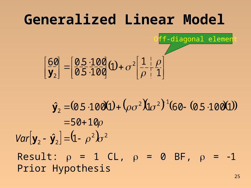
Generalized Linear ModelGeneralized Linear Model

2222

1222

2

2

1ˆ

1050

11005.060111005.0ˆ

11

11005.01005.060

yy

y

y

Var

Off-diagonal element

Result: = 1 CL, = 0 BF, = 1 Prior HypothesisResult: = 1 CL, = 0 BF, = 1 Prior Hypothesis

26

ConclusionConclusion Typical loss reserving methods:

are primitive linear statistical models originated in a bygone deterministic era underutilize the data

Linear statistical models: are BLUE obviate stochastic regressors with covariance have desirable linear properties, especially for

present-valuing fully utilize the data are versatile, of limitless form force the actuary to clarify assumptions

Typical loss reserving methods: are primitive linear statistical models originated in a bygone deterministic era underutilize the data

Linear statistical models: are BLUE obviate stochastic regressors with covariance have desirable linear properties, especially for

present-valuing fully utilize the data are versatile, of limitless form force the actuary to clarify assumptions

27

ReferencesReferencesBarnett, Glen, and Ben Zehnwirth, “Best Estimates for Reserves,” Fall

1998 Forum, 1-54.

Bulmer, M.G., Principles of Statistics, Dover, 1979.

Halliwell, Leigh J., “Loss Prediction by Generalized Least Squares, PCAS LXXXIII (1996), 436-489.

“ , “Statistical and Financial Aspects of Self-Insurance Funding,” Alternative Markets / Self Insurance, 1996, 1-46.

“ , “Conjoint Prediction of Paid and Incurred Losses,” Summer 1997 Forum, 241-379.

“ , “Statistical Models and Credibility,” Winter 1998 Forum, 61-152.

Judge, George G., et al., Introduction to the Theory and Practice of Econometrics, Second Edition, Wiley, 1988.

Pindyck, Robert S., and Daniel L. Rubinfeld, Econometric Models and Economic Forecasts, Fourth Edition, Irwin/McGraw-Hill, 1998.

Barnett, Glen, and Ben Zehnwirth, “Best Estimates for Reserves,” Fall 1998 Forum, 1-54.

Bulmer, M.G., Principles of Statistics, Dover, 1979.

Halliwell, Leigh J., “Loss Prediction by Generalized Least Squares, PCAS LXXXIII (1996), 436-489.

“ , “Statistical and Financial Aspects of Self-Insurance Funding,” Alternative Markets / Self Insurance, 1996, 1-46.

“ , “Conjoint Prediction of Paid and Incurred Losses,” Summer 1997 Forum, 241-379.

“ , “Statistical Models and Credibility,” Winter 1998 Forum, 61-152.

Judge, George G., et al., Introduction to the Theory and Practice of Econometrics, Second Edition, Wiley, 1988.

Pindyck, Robert S., and Daniel L. Rubinfeld, Econometric Models and Economic Forecasts, Fourth Edition, Irwin/McGraw-Hill, 1998.