1 research method lecture 3 (ch4) inferences ©. sampling distribution of ols estimators 4we have...

1

Research MethodResearch Method

Lecture 3 (Ch4)Lecture 3 (Ch4)

InferencesInferences

©

Sampling distribution of Sampling distribution of OLS estimatorsOLS estimators

We have learned that MLR.1-MLR4 will guarantee that OLS estimators are unbiased.

In addition, we have learned that, by adding MLR.5, you can estimate the variance of OLS estimators.

However, in order to conduct hypothesis tests, we need to know the sampling distribution of the OLS estimators.

2

To do so, we introduce one more assumption

Assumption MLR.6

　　 (i) The population error u is independent of explanatory variables, x1,x2,…,xk, and (ii) u~N(0,σ2).

3

Classical Linear Classical Linear AssumptionAssumption

MLR.1 through MLR6 are called the classical linear model (CLM) assumptions.

Note that MLR.6(i) automatically satisfies MLR.4(provided E(u)=0 which we always assume), but MLR.4 does not necessarily indicate MLR.6(i). In this sense, MLR.4 is redundant. However, to emphasize that we are making additional assumption, MLR1 through MLR.6 are called CLM assumptions.

4

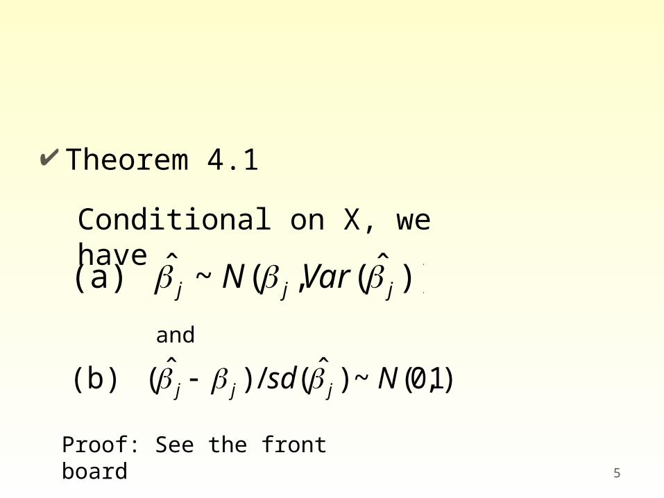
Theorem 4.1

5

))ˆ(,(~ˆ (a) jjj VarN

)1,0(~)ˆ(/)ˆ( (b) Nsd jjj and

Proof: See the front board

Conditional on X, we have

Hypothesis testingHypothesis testing Consider the following multiple linear regression.

y=β0+β1x1+β2x2+….+βkxk+u

Now, I present a well known theorem.

6

Theorem 4.2: t-distribution for the standardized estimators.

Under MLR1 through MLR6 (CLM assumptions) we have

7

1~)ˆ(

ˆ

kn

j

jj tse

This means that the standardized coefficient follows t-distribution with n-k-1 degree of freedom. Proof: See the front board.

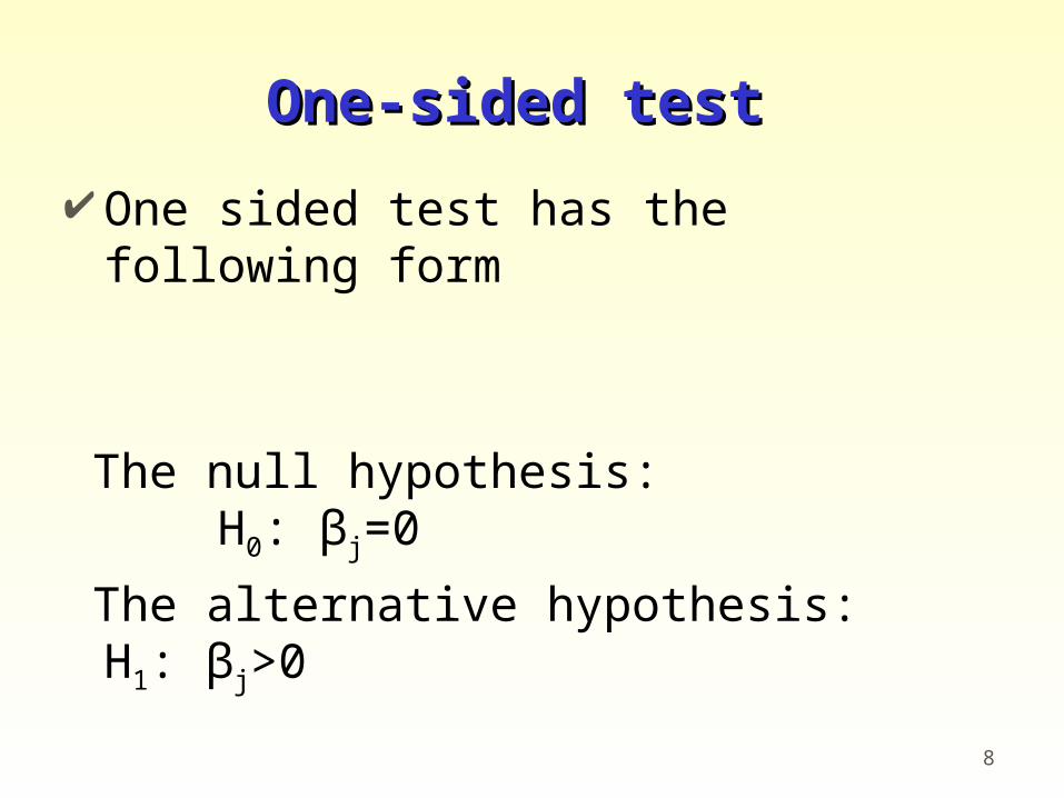
One-sided testOne-sided test

One sided test has the following form

The null hypothesis: H0: βj=0

The alternative hypothesis: H1: βj>0

8

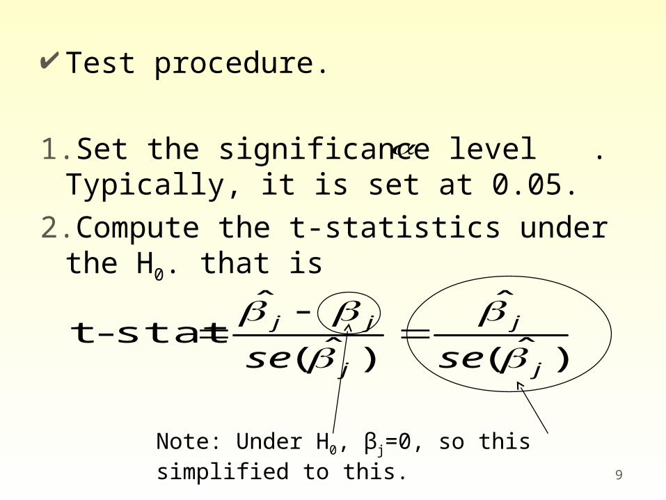
Test procedure.

1.Set the significance level . Typically, it is set at 0.05.

2.Compute the t-statistics under the H0. that is

9

)ˆ(

ˆ

)ˆ(

ˆstat-t

j

j

j

jj

sese

Note: Under H0, βj=0, so this simplified to this.

1

tn-k-1,α

3. Find the cutoff number This cutoff number is illustrated below.

T-distribution with n-k-1 degree of freedom

10

The cutoff number.

4. Reject the null hypothesis if the t-statistic falls in the rejection region. This is illustrated in the next page.

,1 knt

1

tn-k-1,α

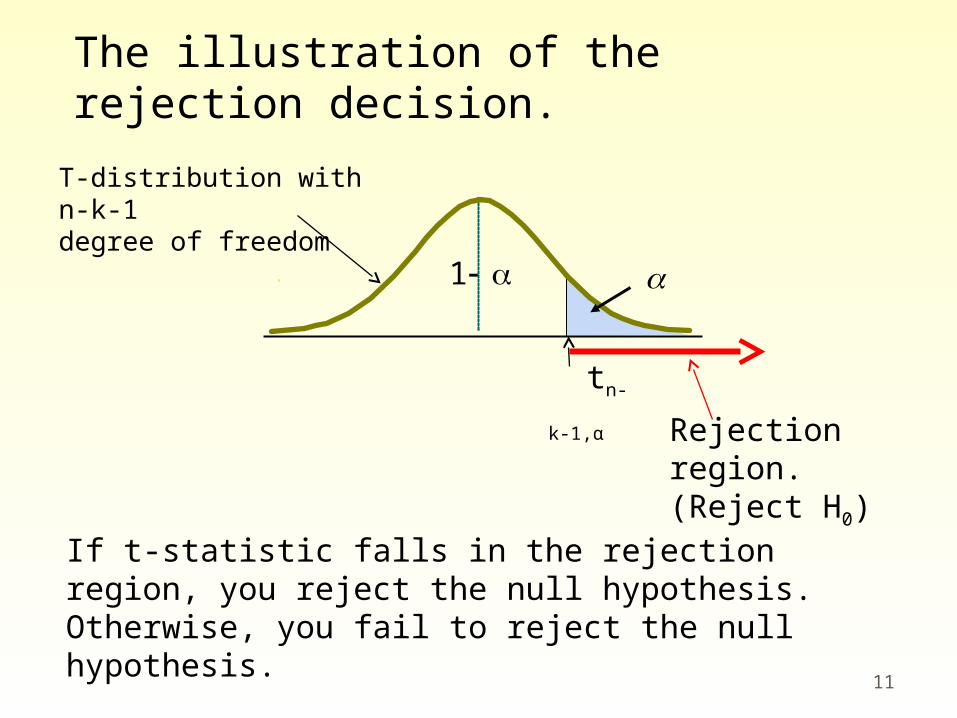
The illustration of the rejection decision.


11

If t-statistic falls in the rejection region, you reject the null hypothesis. Otherwise, you fail to reject the null hypothesis.

Rejection region.(Reject H0)

1

-tn-k-1,α

12

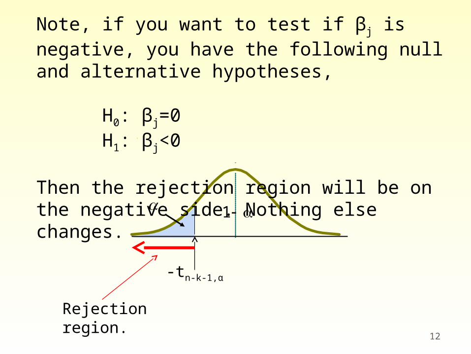
Note, if you want to test if βj is negative, you have the following null and alternative hypotheses, H0: βj=0 H1: βj<0

Then the rejection region will be on the negative side. Nothing else changes.

Rejection region.

ExampleExample

The next slide shows the estimated result of the log salary equation for 338 Japanese economists. (Estimation is done by STATA.)

The estimated regression is

Log(salary)=β0+β1(female)+ δ(other variables)+u

13

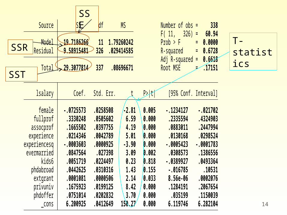
14 _cons 6.200925 .0412649 150.27 0.000 6.119746 6.282104 phdoffer .0751014 .0202832 3.70 0.000 .035199 .1150039 privuniv .1675923 .0199125 8.42 0.000 .1284191 .2067654 extgrant .0001081 .0000506 2.14 0.033 8.56e-06 .0002076 phdabroad .0442625 .0310316 1.43 0.155 -.016785 .10531 kids6 .0051719 .0224497 0.23 0.818 -.0389927 .0493364 evermarried .0847564 .027398 3.09 0.002 .0308573 .1386556experiencesq -.0003603 .0000925 -3.90 0.000 -.0005423 -.0001783 experience .0214346 .0042789 5.01 0.000 .0130168 .0298524 assocprof .1665502 .0397755 4.19 0.000 .0883011 .2447994 fullprof .3330248 .0505602 6.59 0.000 .2335594 .4324903 female -.0725573 .0258508 -2.81 0.005 -.1234127 -.021702 lsalary Coef. Std. Err. t P>|t| [95% Conf. Interval]

Total 29.3077814 337 .08696671 Root MSE = .17151 Adj R-squared = 0.6618 Residual 9.58915481 326 .029414585 R-squared = 0.6728 Model 19.7186266 11 1.79260242 Prob > F = 0.0000 F( 11, 326) = 60.94 Source SS df MS Number of obs = 338

SSE

SSR

SST

T-statistics

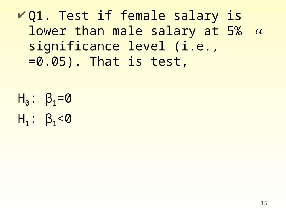
Q1. Test if female salary is lower than male salary at 5% significance level (i.e., =0.05). That is test,

H0: β1=0

H1: β1<0

15

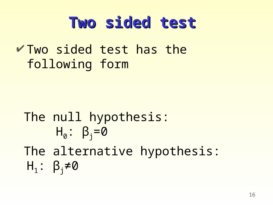
Two sided testTwo sided test

Two sided test has the following form

The null hypothesis: H0: βj=0

The alternative hypothesis: H1: βj≠0

16

Test procedure.

1.Set the significance level . Typically, it is set at 0.05.

2.Compute the t-statistics under the H0. that is

17

)ˆ(

ˆ

)ˆ(

ˆstat-t

j

j

j

jj

sese

Note: Under H0, βj=0, so this simplified to this.

2/1

tn-k-1,α/2

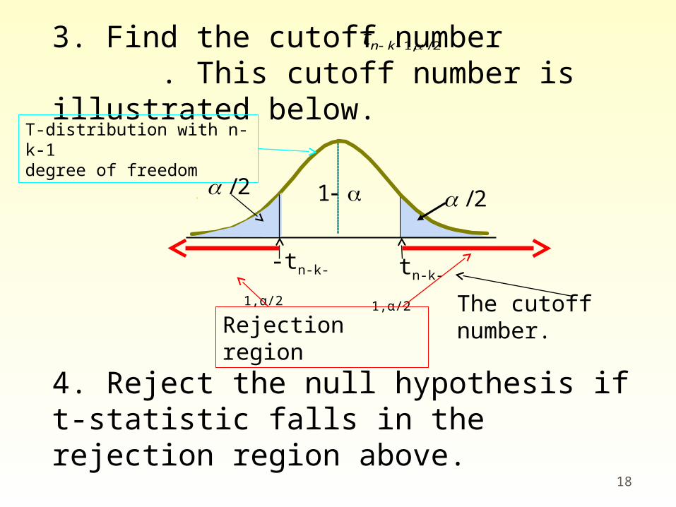
3. Find the cutoff number . This cutoff number is illustrated below.


18

The cutoff number.

4. Reject the null hypothesis if t-statistic falls in the rejection region above.

-tn-k-1,α/2

2/

Rejection region

2/,1 knt

When you reject the null hypothesis βj≠0 using two sided test, we say that the variable xj is statistically significant.

19

ExerciseExercise Consider again the following regression

Log(salary)=β0+β1(female)+ δ(other variables)+u

This time, test if female coefficient is equal to zero or not using two sided test at the 5% significance level. That is, test

H0: β1=0

H1: β1≠0

20



SSE

SSR

SST

The p-valueThe p-value

The p-value is the minimum level of the significance level ( ) at which, the coefficient is statistically significant.

STATA program automatically compute this value for you.

Take a look at the salary regression again.

22



SSE

SSR

SST

P-values

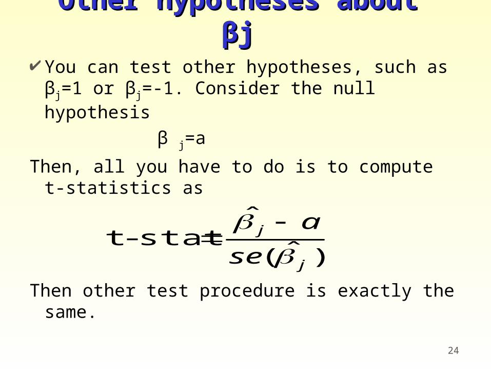
Other hypotheses about Other hypotheses about ββjj

You can test other hypotheses, such as βj=1 or βj=-1. Consider the null hypothesis

β j=a

Then, all you have to do is to compute t-statistics as

Then other test procedure is exactly the same.

24

)ˆ(

ˆstat-t

j

j

se

a

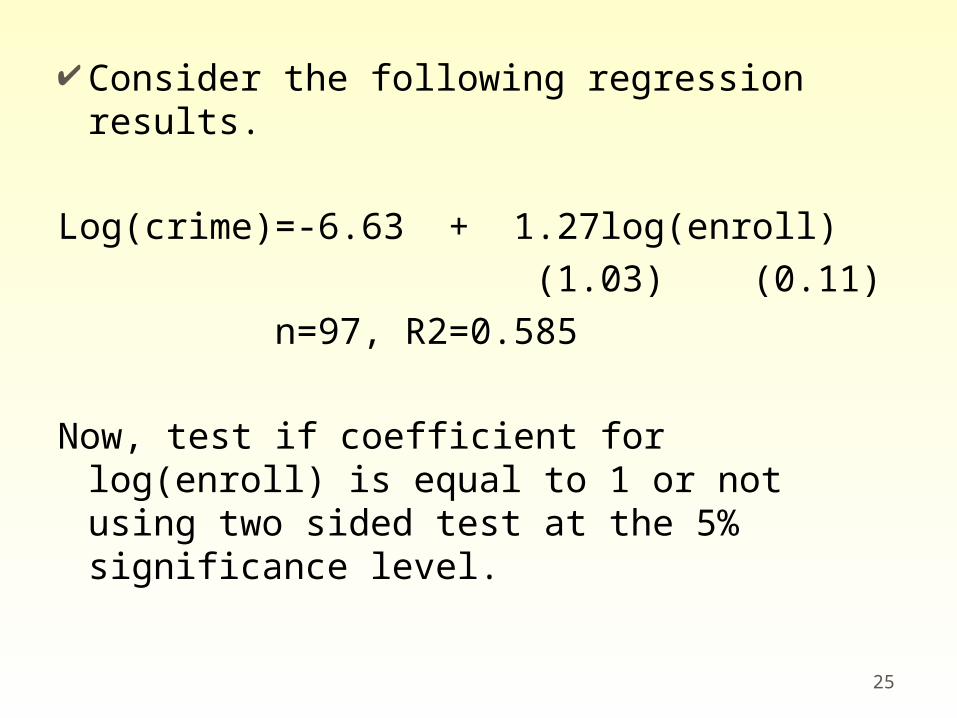
Consider the following regression results.

Log(crime)=-6.63 + 1.27log(enroll) (1.03) (0.11) n=97, R2=0.585

Now, test if coefficient for log(enroll) is equal to 1 or not using two sided test at the 5% significance level.

25

The F-testThe F-testTesting general linear Testing general linear

restrictionsrestrictions You are often interested in more

complicated hypothesis testing.

First, I will show you some examples of such tests using the salary regression example.

26

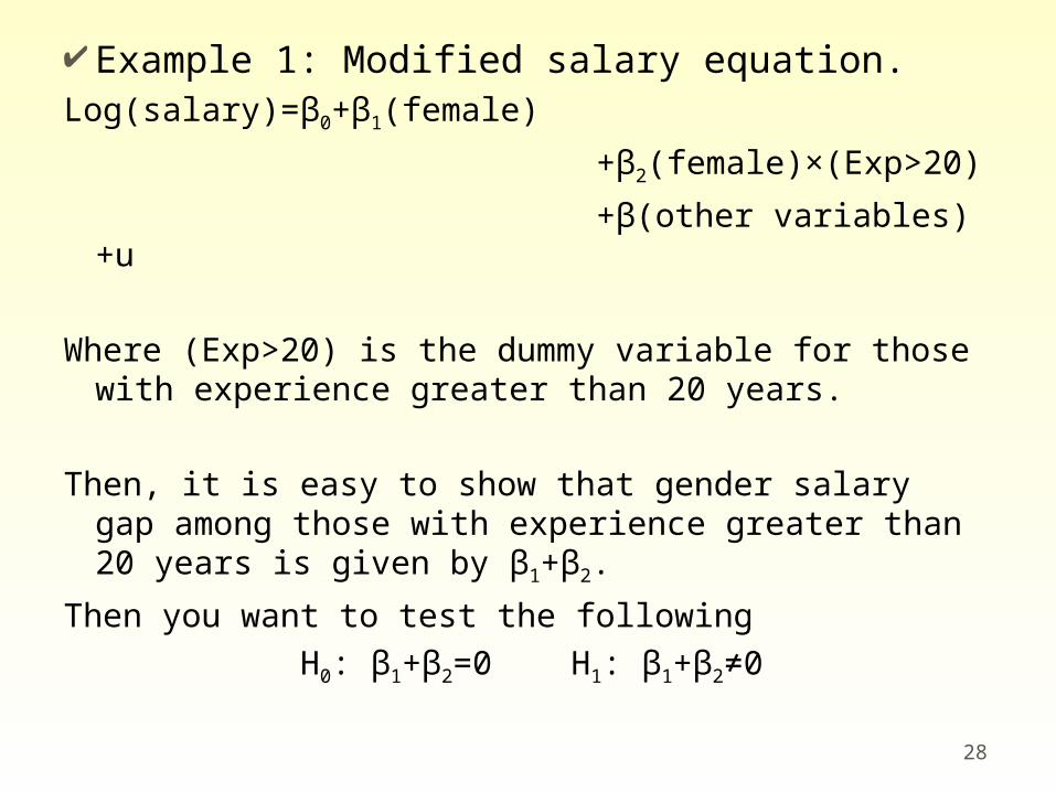
Example 1: Modified salary equation.Log(salary)=β0+β1(female)

+β2(female)×(Exp>20)

+β(other variables)+u

Where (Exp>20) is the dummy variable for those with experience greater than 20 years.

Then, it is easy to show that gender salary gap among those with experience greater than 20 years is given by β1+β2.

Then you want to test the following H0: β1+β2=0 H1: β1+β2≠0

28

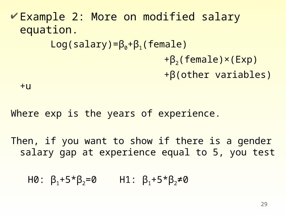
Example 2: More on modified salary equation.

Log(salary)=β0+β1(female)

+β2(female)×(Exp)

+β(other variables)+u

Where exp is the years of experience.

Then, if you want to show if there is a gender salary gap at experience equal to 5, you test

H0: β1+5*β2=0 H1: β1+5*β2≠0 29

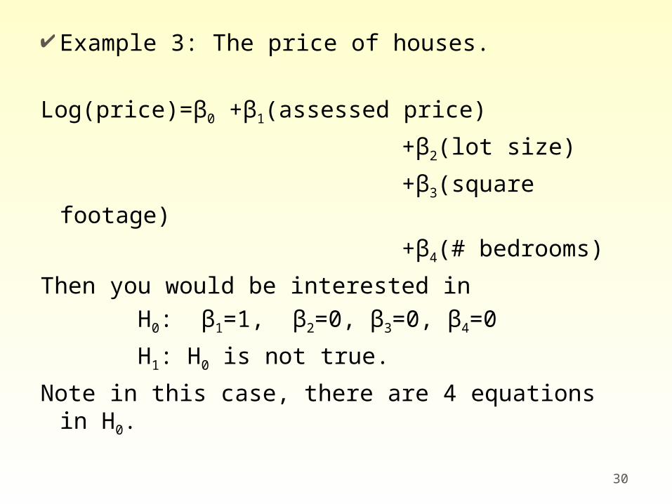
Example 3: The price of houses.

Log(price)=β0 +β1(assessed price)

+β2(lot size)

+β3(square footage)

+β4(# bedrooms)

Then you would be interested in H0: β1=1, β2=0, β3=0, β4=0

H1: H0 is not true.

Note in this case, there are 4 equations in H0.

30

The procedure for F-testThe procedure for F-test

Linear restrictions are tested using F-test. The general procedure can be explained using the following example.

Y= β0+β1x1+β2x2+β3x3+β4x4+u --------------(1)

Suppose you want to test H0: β1=1, β2=β3, β4=0

H1: H0 is not true

31

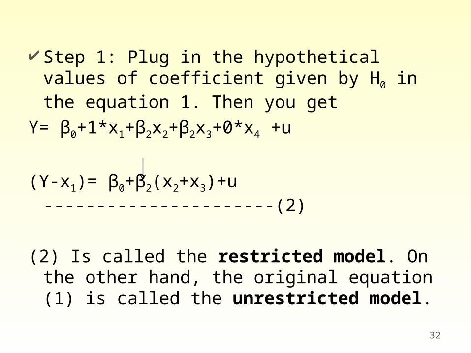
Step 1: Plug in the hypothetical values of coefficient given by H0 in the equation 1. Then you get

Y= β0+1*x1+β2x2+β2x3+0*x4 +u

(Y-x1)= β0+β2(x2+x3)+u ----------------------(2)

(2) Is called the restricted model. On the other hand, the original equation (1) is called the unrestricted model.

32

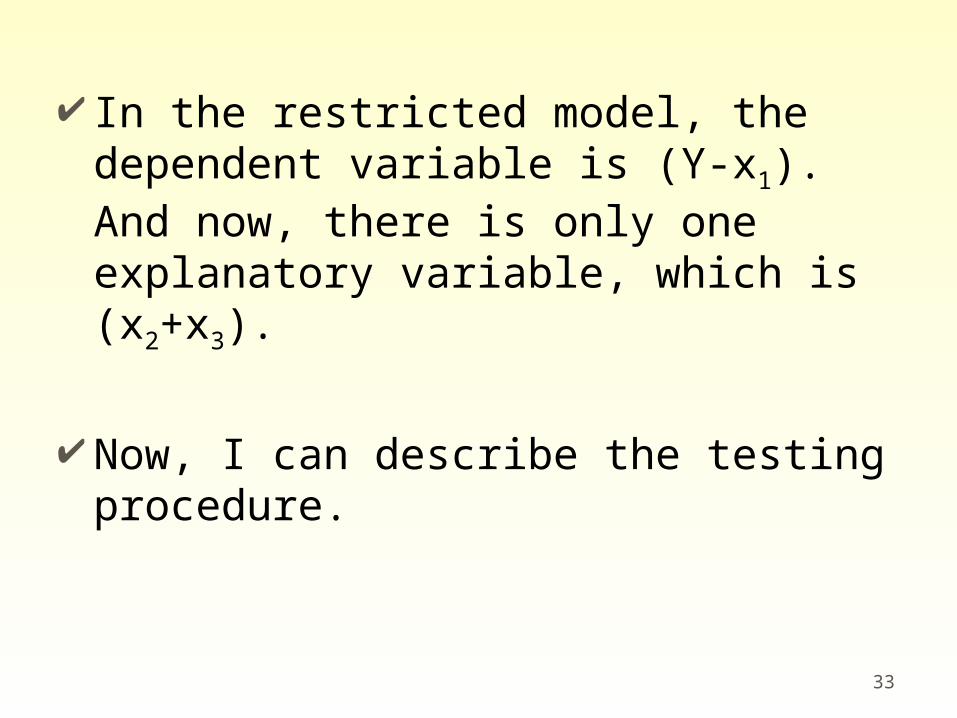
In the restricted model, the dependent variable is (Y-x1). And now, there is only one explanatory variable, which is (x2+x3).

Now, I can describe the testing procedure.

33

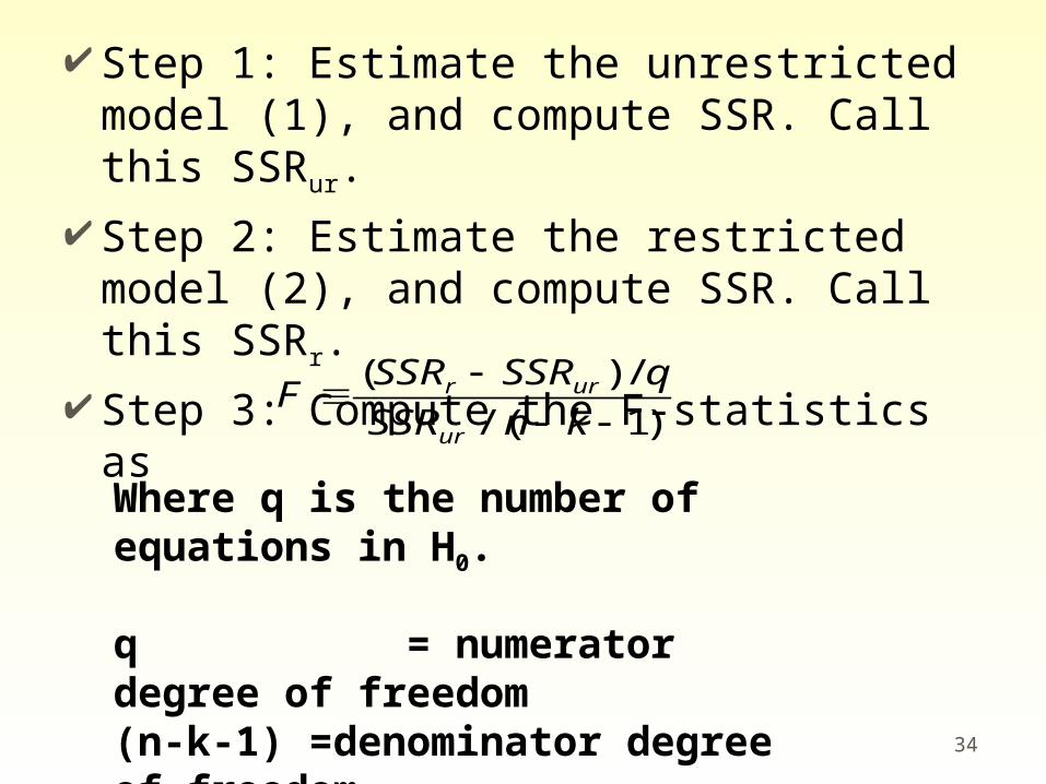
Step 1: Estimate the unrestricted model (1), and compute SSR. Call this SSRur.

Step 2: Estimate the restricted model (2), and compute SSR. Call this SSRr.

Step 3: Compute the F-statistics as

34

)1/(

/)(

knSSR

qSSRSSRF

ur

urr

Where q is the number of equations in H0.

q = numerator degree of freedom(n-k-1) =denominator degree of freedom

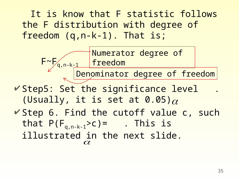
It is know that F statistic follows the F distribution with degree of freedom (q,n-k-1). That is;

F~Fq,n-k-1

Step5: Set the significance level . (Usually, it is set at 0.05)

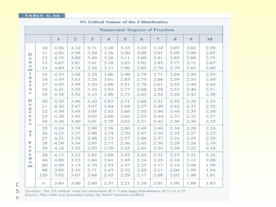
Step 6. Find the cutoff value c, such that P(Fq,n-k-1>c)= . This is illustrated in the next slide.

35

Numerator degree of freedom

Denominator degree of freedom

36

c

1-

The density of Fq,n-k-1

Rejection region

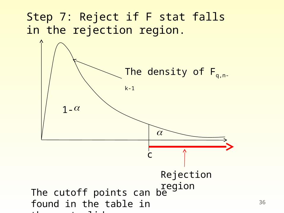
Step 7: Reject if F stat falls in the rejection region.

The cutoff points can be found in the table in the next slide.

ExampleExample

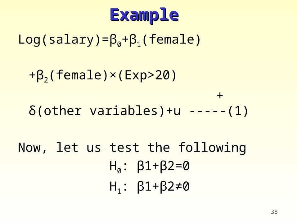
Log(salary)=β0+β1(female)

+β2(female)×(Exp>20)

+ δ(other variables)+u -----(1)

Now, let us test the following H0: β1+β2=0

H1: β1+β2≠038

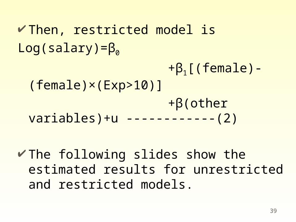
Then, restricted model isLog(salary)=β0

+β1[(female)-(female)×(Exp>10)]

+β(other variables)+u ------------(2)

The following slides show the estimated results for unrestricted and restricted models.

39

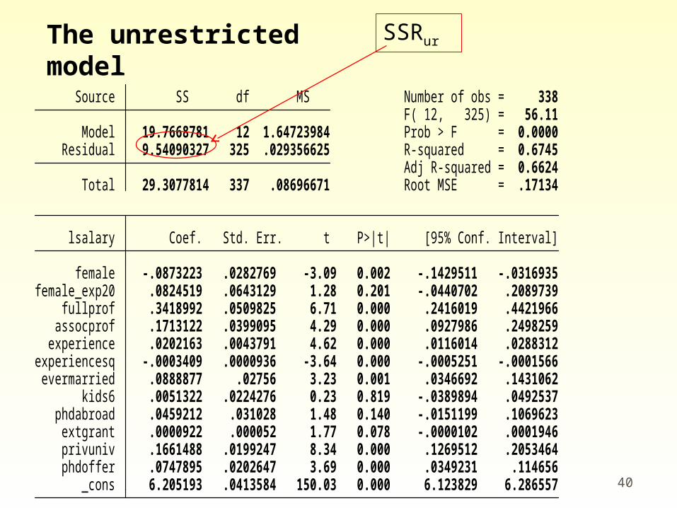
40 _cons 6.205193 .0413584 150.03 0.000 6.123829 6.286557 phdoffer .0747895 .0202647 3.69 0.000 .0349231 .114656 privuniv .1661488 .0199247 8.34 0.000 .1269512 .2053464 extgrant .0000922 .000052 1.77 0.078 -.0000102 .0001946 phdabroad .0459212 .031028 1.48 0.140 -.0151199 .1069623 kids6 .0051322 .0224276 0.23 0.819 -.0389894 .0492537 evermarried .0888877 .02756 3.23 0.001 .0346692 .1431062experiencesq -.0003409 .0000936 -3.64 0.000 -.0005251 -.0001566 experience .0202163 .0043791 4.62 0.000 .0116014 .0288312 assocprof .1713122 .0399095 4.29 0.000 .0927986 .2498259 fullprof .3418992 .0509825 6.71 0.000 .2416019 .4421966female_exp20 .0824519 .0643129 1.28 0.201 -.0440702 .2089739 female -.0873223 .0282769 -3.09 0.002 -.1429511 -.0316935 lsalary Coef. Std. Err. t P>|t| [95% Conf. Interval]


The unrestricted model SSRur

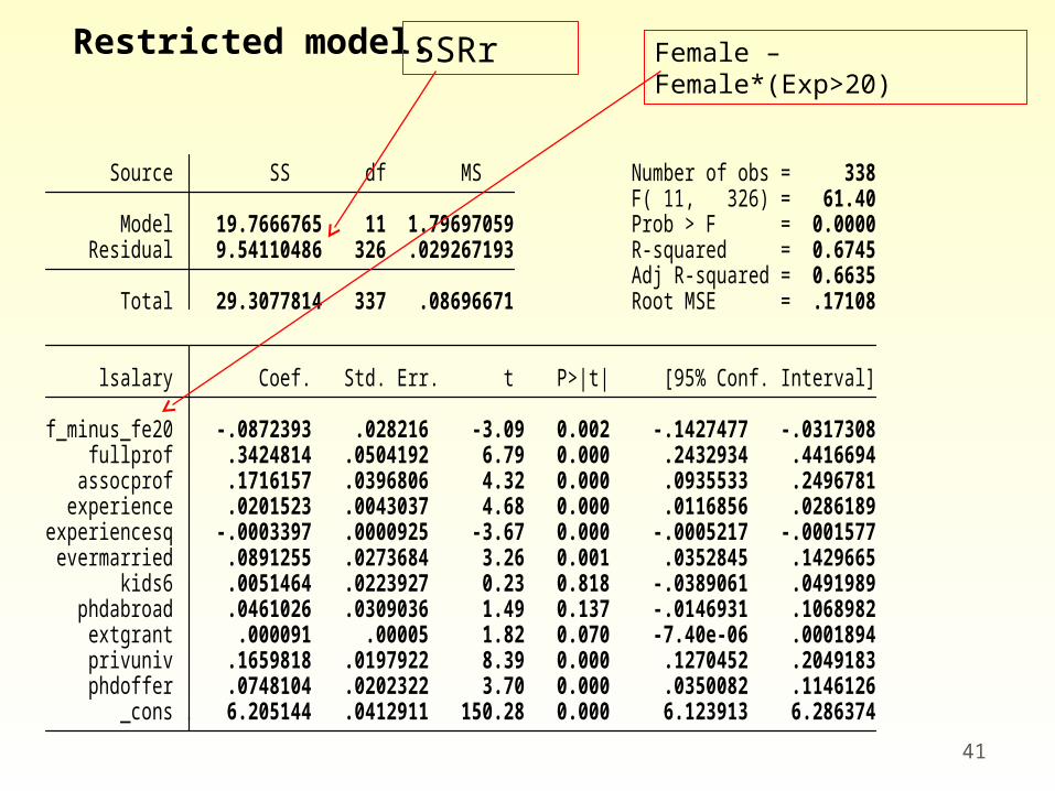
41 _cons 6.205144 .0412911 150.28 0.000 6.123913 6.286374 phdoffer .0748104 .0202322 3.70 0.000 .0350082 .1146126 privuniv .1659818 .0197922 8.39 0.000 .1270452 .2049183 extgrant .000091 .00005 1.82 0.070 -7.40e-06 .0001894 phdabroad .0461026 .0309036 1.49 0.137 -.0146931 .1068982 kids6 .0051464 .0223927 0.23 0.818 -.0389061 .0491989 evermarried .0891255 .0273684 3.26 0.001 .0352845 .1429665experiencesq -.0003397 .0000925 -3.67 0.000 -.0005217 -.0001577 experience .0201523 .0043037 4.68 0.000 .0116856 .0286189 assocprof .1716157 .0396806 4.32 0.000 .0935533 .2496781 fullprof .3424814 .0504192 6.79 0.000 .2432934 .4416694f_minus_fe20 -.0872393 .028216 -3.09 0.002 -.1427477 -.0317308 lsalary Coef. Std. Err. t P>|t| [95% Conf. Interval]


Restricted model. SSRr Female –Female*(Exp>20)

Since we have only one equation in H0, q=1. And you can see that (n-k-1)=(338-12-1)=325

F=[(9.54110486 -9.54090327)/1]/[9.54090327/325] =0.0068

The cutoff point at 5% significance level is 3.84. Since F-stat does not falls in the rejection, we fail

to reject the null hypothesis. In other words, we did not find evidence that there is a gender gap among those with experience greater than 20 years.

42

In fact, STATA does F-test automatically.

44

Prob > F = 0.9340 F( 1, 325) = 0.01

( 1) female + female_exp20 = 0

. test female + female_exp20=0

. delimiter now cr. #delimit cr

_cons 6.205193 .0413584 150.03 0.000 6.123829 6.286557 phdoffer .0747895 .0202647 3.69 0.000 .0349231 .114656 privuniv .1661488 .0199247 8.34 0.000 .1269512 .2053464 extgrant .0000922 .000052 1.77 0.078 -.0000102 .0001946 phdabroad .0459212 .031028 1.48 0.140 -.0151199 .1069623 kids6 .0051322 .0224276 0.23 0.819 -.0389894 .0492537 evermarried .0888877 .02756 3.23 0.001 .0346692 .1431062experiencesq -.0003409 .0000936 -3.64 0.000 -.0005251 -.0001566 experience .0202163 .0043791 4.62 0.000 .0116014 .0288312 assocprof .1713122 .0399095 4.29 0.000 .0927986 .2498259 fullprof .3418992 .0509825 6.71 0.000 .2416019 .4421966female_exp20 .0824519 .0643129 1.28 0.201 -.0440702 .2089739 female -.0873223 .0282769 -3.09 0.002 -.1429511 -.0316935 lsalary Coef. Std. Err. t P>|t| [95% Conf. Interval]


After estimation, type this command

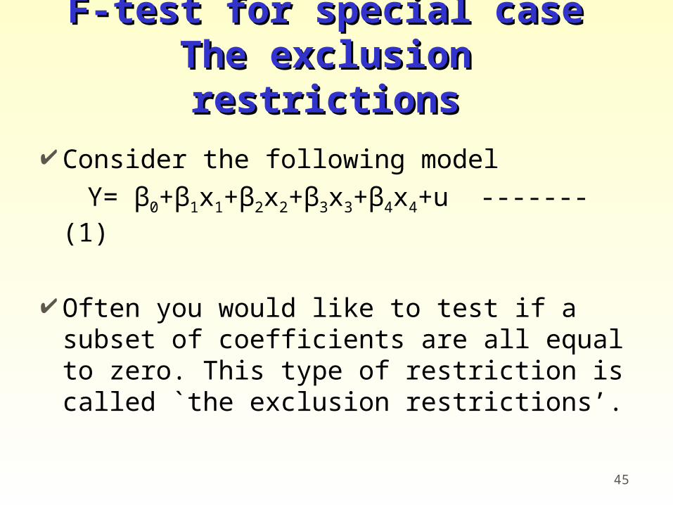
F-test for special caseF-test for special caseThe exclusion restrictionsThe exclusion restrictions

Consider the following model Y= β0+β1x1+β2x2+β3x3+β4x4+u -------

(1)

Often you would like to test if a subset of coefficients are all equal to zero. This type of restriction is called `the exclusion restrictions’.

45

Suppose you want to test if β2,β3,β4 are jointly equal to zero. Then, you test

H0 : β2=0, β3=0, β4=0

H1: H0 is not true.

46

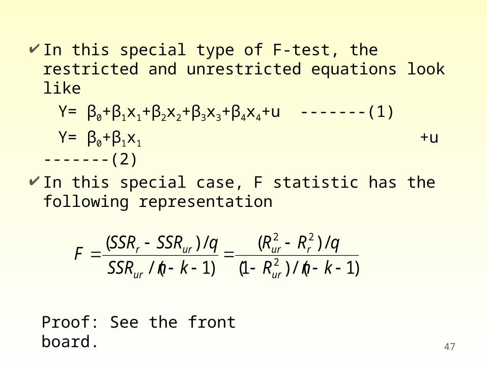
In this special type of F-test, the restricted and unrestricted equations look like

Y= β0+β1x1+β2x2+β3x3+β4x4+u -------(1)

Y= β0+β1x1 +u -------(2) In this special case, F statistic has the

following representation

47

)1/()1(

/)(

)1/(

/)(2

22

knR

qRR

knSSR

qSSRSSRF

ur

rur

ur

urr

Proof: See the front board.

When we reject this type of null hypothesis, we say x2, x3 and x4 are jointly significant.

48

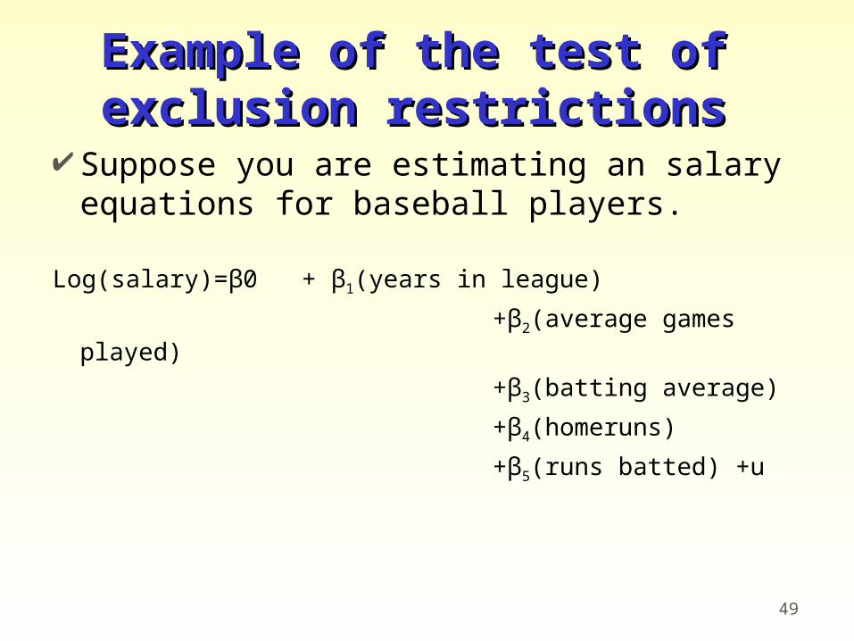
Example of the test of Example of the test of exclusion restrictionsexclusion restrictions

Suppose you are estimating an salary equations for baseball players.

Log(salary)=β0 + β1(years in league)

+β2(average games played)

+β3(batting average)

+β4(homeruns)

+β5(runs batted) +u

49

Do batting average, homeruns and runs batted matters for salary after years in league and average games played are controlled for? To answer to this question, you test

H0: β3=0, β4=0, β5=0

H1: H0 is not true.

50

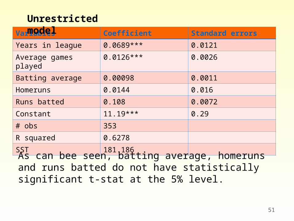
Variables Coefficient Standard errors

Years in league 0.0689*** 0.0121

Average games played

0.0126*** 0.0026

Batting average 0.00098 0.0011

Homeruns 0.0144 0.016

Runs batted 0.108 0.0072

Constant 11.19*** 0.29

# obs 353

R squared 0.6278

SST 181.186

51

As can bee seen, batting average, homeruns and runs batted do not have statistically significant t-stat at the 5% level.

Unrestricted model

The F stat isF=[(198.311-181.186)/3]/[181.186/(353-5-

1)]=10.932The cutoff number of about 2.60. So we reject the

null hypothesis at 5% significance level. This is an reminder that even if each coefficient is individually insignificant, they may be jointly significant.

52

Variables Coefficient Standard errors

Years in league 0.0713*** 0.0125

Average games played

0.0202*** 0.0013

Constant 11.22*** 0.11

# obs 353

R squared 0.5971

SST 198.311

Restricted model

1 research method lecture 3 (ch4) inferences ©. sampling distribution of ols estimators 4we have...

Documents

following h

null hypothesis

assumption assumption

alternative hypothesis

variables u

hypothesis tests

years of experience

standardized estimators