1-sample % defective test - minitab · 2019-04-18 · 1-sample % defective test 4 to help interpret...

WWW.MINITAB.COM

MINITAB ASSISTANT WHITE PAPER

This paper explains the research conducted by Minitab statisticians to develop the methods and

data checks used in the Assistant in Minitab Statistical Software.

1-Sample % Defective Test

Overview A test for 1-proportion is used to determine whether a proportion differs from a target value. In

quality analysis, the test is often used when a product or service is characterized as defective or

not defective to determine whether the percentage of defective items significantly differs from a

target % defective.

The Minitab Assistant includes a 1-Sample % Defective Test. The data collected for the test are

the number of defective items in a sample, which is assumed to be the observed value of a

binomial random variable. The Assistant uses exact methods to calculate the hypothesis test

results and the confidence intervals; therefore, the actual Type I error rate should be near the

level of significance (alpha) specified for the test and no further investigation is required.

However, the power and sample size analysis for the 1-Sample % Defective test is based on an

approximation and we need to evaluate it for accuracy.

In this paper we investigate the methodology used to evaluate power and sample size for the

1-sample % defective test, comparing the theoretical power of the approximate method with

the actual power of the exact test.

We also describe how we established a guideline to help you evaluate whether your sample size

is large enough to detect whether the percentage of defective items differs from a target

% defective. The Assistant automatically performs a check on the sample size and reports the

findings in the Report Card.

The 1-Sample % Defective Test also depends on other assumptions. See Appendix A for details.

1-SAMPLE % DEFECTIVE TEST 2

1-sample % defective method

Performance of theoretical power function The Assistant performs the hypothesis test for a single Bernoulli population proportion

(% defectives) using exact (likelihood ratio) methods. However, because the power function of

this exact test is not easily derived, the power function is approximated using the theoretical

power function of the corresponding normal approximation test.

Objective

We wanted to determine whether we could use the theoretical power function based on the

normal approximation test to evaluate the power and sample size requirements for the

1-Sample % Defective test in the Assistant. To do this, we needed to evaluate whether this

theoretical power function accurately reflects the actual power of the exact (likelihood ratio) test.

Method

The test statistic, p-value, and confidence interval for the exact (likelihood ratio) test are defined

in Appendix B. The theoretical power function based on the normal approximation is defined in

Appendix C. Based on these definitions, we performed simulations to estimate the actual power

levels (which we refer to as simulated power levels) using the exact test.

To perform the simulations, we generated random samples of various sizes from several

Bernoulli populations. For each Bernoulli population, we performed the exact test on each of

10,000 sample replicates. For each sample size, we calculated the simulated power of the test to

detect a given difference as the fraction of the 10,000 samples for which the test is significant.

For comparison, we also calculated the corresponding theoretical power based on the normal

approximation test. If the approximation works well, the theoretical and simulated power levels

should be close. For more details, see Appendix D.

Results

Our simulations showed that, in general, the theoretical power function of the normal

approximation test and the simulated power function of the exact (likelihood ratio) test are

nearly equal. Therefore, the Assistant uses the theoretical power function of the normal

approximation test to estimate the samples sizes needed to ensure that the exact test has

sufficient power to detect practically important differences in the percentage of defectives.


Data checks

Sample size Typically, a hypothesis test is performed to gather evidence to reject the null hypothesis of “no

difference”. If the sample is too small, the power of the test may not be adequate to detect a

difference that actually exists, which results in a Type II error. It is therefore crucial to ensure that

the sample sizes are sufficiently large to detect practically important differences with high

probability.

Objective

If the data does not provide sufficient evidence to reject the null hypothesis, we wanted to

determine whether the sample sizes are large enough for the test to detect practical differences

of interest with high probability. Although the objective of sample size planning is to ensure that

sample sizes are large enough to detect important differences with high probability, they should

not be so large that meaningless differences become statistically significant with high

probability.

Method

The power and sample size analysis for the 1-Sample % Defective test is based upon the

theoretical power function using the normal approximation, which provides a good estimate of

the actual power of the exact test (see the 1-sample % defective method section above). When

the target % defective is given, the theoretical power function depends upon the sample size

and the difference that you want to detect.

Results

When the data does not provide enough evidence against the null hypothesis, the Assistant

calculates practical differences that can be detected with an 80% and a 90% probability for the

given sample size. In addition, if the user provides a particular practical difference of interest, the

Assistant calculates sample sizes that yield an 80% and a 90% chance of detection of the

difference.


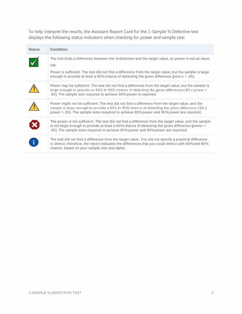
To help interpret the results, the Assistant Report Card for the 1-Sample % Defective test

displays the following status indicators when checking for power and sample size:

Status Condition

The test finds a difference between the % defective and the target value, so power is not an issue.

OR

Power is sufficient. The test did not find a difference from the target value, but the sample is large enough to provide at least a 90% chance of detecting the given difference (pow

Power may be sufficient. The test did not find a difference from the target value, but the sample is

.90). The sample size required to achieve 90% power is reported.

Power might not be sufficient. The test did not find a difference from the target value, and the

power < .80). The sample sizes required to achieve 80% power and 90% power are reported.

The power is not sufficient. The test did not find a difference from the target value, and the sample is not large enough to provide at least a 60% chance of detecting the given difference (power < .60). The sample sizes required to achieve 80% power and 90% power are reported.

The test did not find a difference from the target value. You did not specify a practical difference to detect; therefore, the report indicates the differences that you could detect with 80% and 90% chance, based on your sample size and alpha.


References Arnold, S.F. (1990). Mathematical statistics. Englewood Cliffs, NJ: Prentice Hall, Inc.

Casella, G., & Berger, R.L. (1990). Statistical inference. Pacific Grove, CA: Wadsworth, Inc.


Appendix A: Additional assumptions for 1-sample % defective The 1-Sample % Defective test is based on the following assumptions:

The data consist of n distinct items, with each item classified as either defective or not

defective.

The probability of an item being defective is the same for each item within a sample.

The likelihood of an item being defective is not affected by whether another item is

defective or not.

These assumptions cannot be verified in the data checks of the Report Card because summary

data, rather than raw data, is entered for this test.


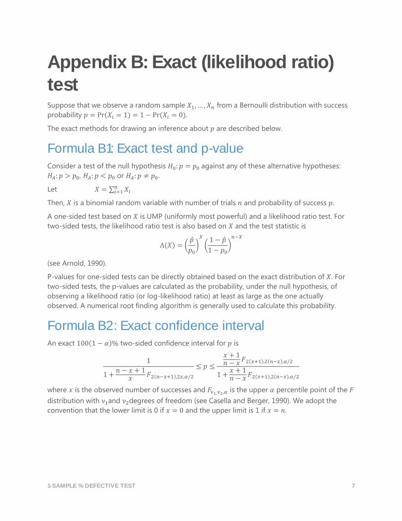
Appendix B: Exact (likelihood ratio) test Suppose that we observe a random sample 𝑋1, … , 𝑋𝑛 from a Bernoulli distribution with success

probability 𝑝 = Pr(𝑋𝑖 = 1) = 1 − Pr(𝑋𝑖 = 0).

The exact methods for drawing an inference about 𝑝 are described below.

Formula B1: Exact test and p-value Consider a test of the null hypothesis 𝐻0: 𝑝 = 𝑝0 against any of these alternative hypotheses:

𝐻𝐴: 𝑝 > 𝑝0, 𝐻𝐴: 𝑝 < 𝑝0 or 𝐻𝐴: 𝑝 ≠ 𝑝0.

Let 𝑋 = ∑ 𝑋𝑖𝑛𝑖=1

Then, 𝑋 is a binomial random variable with number of trials 𝑛 and probability of success 𝑝.

A one-sided test based on 𝑋 is UMP (uniformly most powerful) and a likelihood ratio test. For

two-sided tests, the likelihood ratio test is also based on 𝑋 and the test statistic is

Λ(𝑋) = (�̂�

𝑝0)

𝑋

(1 − �̂�

1 − 𝑝0)

𝑛−𝑋

(see Arnold, 1990).

P-values for one-sided tests can be directly obtained based on the exact distribution of 𝑋. For

two-sided tests, the p-values are calculated as the probability, under the null hypothesis, of

observing a likelihood ratio (or log-likelihood ratio) at least as large as the one actually

observed. A numerical root finding algorithm is generally used to calculate this probability.

Formula B2: Exact confidence interval An exact 100(1 − 𝛼)% two-sided confidence interval for 𝑝 is

1

1 +𝑛 − 𝑥 + 1

𝑥 𝐹2(𝑛−𝑥+1),2𝑥,𝛼/2

≤ 𝑝 ≤

𝑥 + 1𝑛 − 𝑥 𝐹2(𝑥+1),2(𝑛−𝑥),𝛼/2

1 +𝑥 + 1𝑛 − 𝑥 𝐹2(𝑥+1),2(𝑛−𝑥),𝛼/2

where 𝑥 is the observed number of successes and 𝐹𝜈1,𝜈2,𝛼 is the upper 𝛼 percentile point of the 𝐹

distribution with 𝜈1and 𝜈2degrees of freedom (see Casella and Berger, 1990). We adopt the

convention that the lower limit is 0 if 𝑥 = 0 and the upper limit is 1 if 𝑥 = 𝑛.


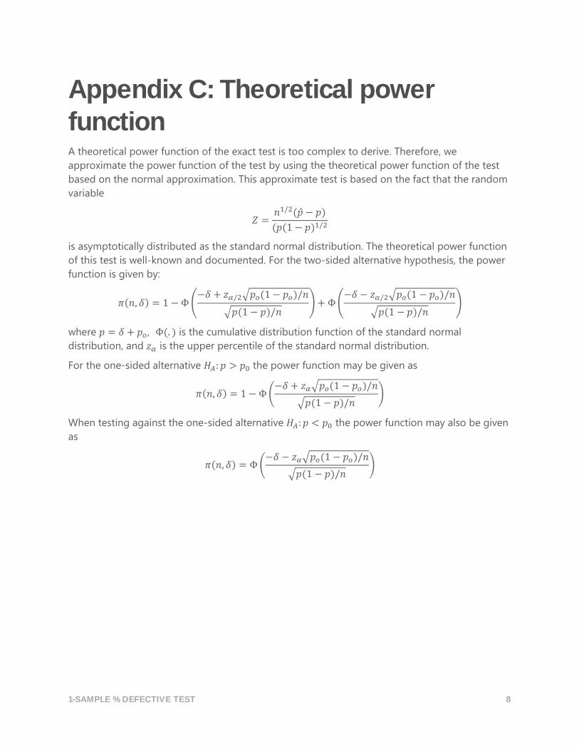
Appendix C: Theoretical power function

A theoretical power function of the exact test is too complex to derive. Therefore, we

approximate the power function of the test by using the theoretical power function of the test

based on the normal approximation. This approximate test is based on the fact that the random

variable

𝑍 =𝑛1/2(�̂� − 𝑝)

(𝑝(1 − 𝑝)1/2

is asymptotically distributed as the standard normal distribution. The theoretical power function

of this test is well-known and documented. For the two-sided alternative hypothesis, the power

function is given by:

𝜋(𝑛, 𝛿) = 1 − Φ (−𝛿 + 𝑧𝛼/2√𝑝𝑜(1 − 𝑝𝑜)/𝑛

√𝑝(1 − 𝑝)/𝑛) + Φ (

−𝛿 − 𝑧𝛼/2√𝑝𝑜(1 − 𝑝𝑜)/𝑛

√𝑝(1 − 𝑝)/𝑛)

where 𝑝 = 𝛿 + 𝑝𝑜, Φ(. ) is the cumulative distribution function of the standard normal

distribution, and 𝑧𝛼 is the upper percentile of the standard normal distribution.

For the one-sided alternative 𝐻𝐴: 𝑝 > 𝑝0 the power function may be given as

𝜋(𝑛, 𝛿) = 1 − Φ (−𝛿 + 𝑧𝛼√𝑝𝑜(1 − 𝑝𝑜)/𝑛

√𝑝(1 − 𝑝)/𝑛)

When testing against the one-sided alternative 𝐻𝐴: 𝑝 < 𝑝0 the power function may also be given

as

𝜋(𝑛, 𝛿) = Φ (−𝛿 − 𝑧𝛼√𝑝𝑜(1 − 𝑝𝑜)/𝑛

√𝑝(1 − 𝑝)/𝑛)


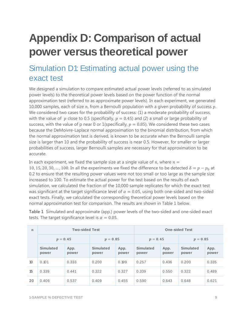
Appendix D: Comparison of actual power versus theoretical power

Simulation D1: Estimating actual power using the exact test We designed a simulation to compare estimated actual power levels (referred to as simulated

power levels) to the theoretical power levels based on the power function of the normal

approximation test (referred to as approximate power levels). In each experiment, we generated

10,000 samples, each of size 𝑛, from a Bernoulli population with a given probability of success 𝑝.

We considered two cases for the probability of success: (1) a moderate probability of success,

with the value of 𝑝 close to 0.5 (specifically, 𝑝 = 0.45) and (2) a small or large probability of

success, with the value of p near 0 or 1(specifically, 𝑝 = 0.85). We considered these two cases

because the DeMoivre-Laplace normal approximation to the binomial distribution, from which

the normal approximation test is derived, is known to be accurate when the Bernoulli sample

size is larger than 10 and the probability of success is near 0.5. However, for smaller or larger

probabilities of success, larger Bernoulli samples are necessary for that approximation to be

accurate.

In each experiment, we fixed the sample size at a single value of 𝑛, where 𝑛 =

10, 15, 20, 30, … , 100. In all the experiments we fixed the difference to be detected 𝛿 = 𝑝 − 𝑝0 at

0.2 to ensure that the resulting power values were not too small or too large as the sample size

increased to 100. To estimate the actual power for the test based on the results of each

simulation, we calculated the fraction of the 10,000 sample replicates for which the exact test

was significant at the target significance level of 𝛼 = 0.05, using both one-sided and two-sided

exact tests. Finally, we calculated the corresponding theoretical power levels based on the

normal approximation test for comparison. The results are shown in Table 1 below.

Table 1 Simulated and approximate (app.) power levels of the two-sided and one-sided exact

tests. The target significance level is 𝛼 = 0.05.

𝒏 Two-sided Test One-sided Test

𝒑 = 𝟎. 𝟒𝟓 𝒑 = 𝟎. 𝟖𝟓 𝒑 = 𝟎. 𝟒𝟓 𝒑 = 𝟎. 𝟖𝟓

Simulated power

App. power

Simulated power

App. power

Simulated power

App. power

Simulated power

App. power

10 0.101 0.333 0.200 0.199 0.257 0.436 0.200 0.335

15 0.339 0.441 0.322 0.327 0.339 0.550 0.322 0.489

20 0.406 0.537 0.409 0.455 0.590 0.643 0.648 0.621


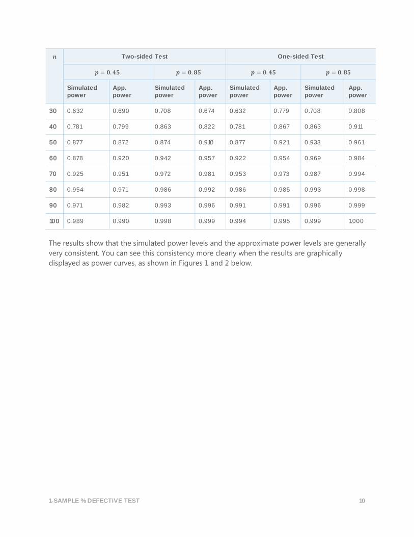
𝒏 Two-sided Test One-sided Test

𝒑 = 𝟎. 𝟒𝟓 𝒑 = 𝟎. 𝟖𝟓 𝒑 = 𝟎. 𝟒𝟓 𝒑 = 𝟎. 𝟖𝟓

Simulated power

App. power

Simulated power

App. power

Simulated power

App. power

Simulated power

App. power

30 0.632 0.690 0.708 0.674 0.632 0.779 0.708 0.808

40 0.781 0.799 0.863 0.822 0.781 0.867 0.863 0.911

50 0.877 0.872 0.874 0.910 0.877 0.921 0.933 0.961

60 0.878 0.920 0.942 0.957 0.922 0.954 0.969 0.984

70 0.925 0.951 0.972 0.981 0.953 0.973 0.987 0.994

80 0.954 0.971 0.986 0.992 0.986 0.985 0.993 0.998

90 0.971 0.982 0.993 0.996 0.991 0.991 0.996 0.999

100 0.989 0.990 0.998 0.999 0.994 0.995 0.999 1.000

The results show that the simulated power levels and the approximate power levels are generally

very consistent. You can see this consistency more clearly when the results are graphically

displayed as power curves, as shown in Figures 1 and 2 below.


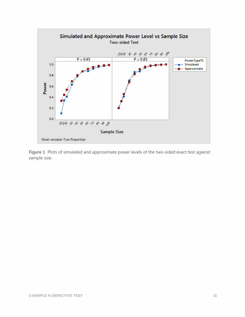
Figure 1 Plots of simulated and approximate power levels of the two-sided exact test against

sample size.


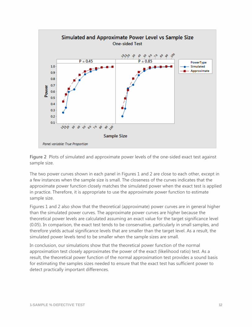
Figure 2 Plots of simulated and approximate power levels of the one-sided exact test against

sample size.

The two power curves shown in each panel in Figures 1 and 2 are close to each other, except in

a few instances when the sample size is small. The closeness of the curves indicates that the

approximate power function closely matches the simulated power when the exact test is applied

in practice. Therefore, it is appropriate to use the approximate power function to estimate

sample size.

Figures 1 and 2 also show that the theoretical (approximate) power curves are in general higher

than the simulated power curves. The approximate power curves are higher because the

theoretical power levels are calculated assuming an exact value for the target significance level

(0.05). In comparison, the exact test tends to be conservative, particularly in small samples, and

therefore yields actual significance levels that are smaller than the target level. As a result, the

simulated power levels tend to be smaller when the sample sizes are small.

In conclusion, our simulations show that the theoretical power function of the normal

approximation test closely approximates the power of the exact (likelihood ratio) test. As a

result, the theoretical power function of the normal approximation test provides a sound basis

for estimating the samples sizes needed to ensure that the exact test has sufficient power to

detect practically important differences.


© 2015, 2017 Minitab Inc. All rights reserved.

Minitab®, Quality. Analysis. Results.® and the Minitab® logo are all registered trademarks of Minitab,

Inc., in the United States and other countries. See minitab.com/legal/trademarks for more information.

1-sample % defective test - minitab · 2019-04-18 · 1-sample % defective test 4 to help interpret...

Documents