1 Some Mathematical Ideas and their Appli-

cations

1.1 An Idea from Analysis

Spectral theory is one of most fruitful ideas of analysis and has applicationsto probability theory. We do not intend to give a sophisticated treatment ofthe spectral theorem, rather we loosely explain the general idea and apply itto a random walk problems. Even understanding the broad outlines of thetheory is a useful mathematical tool.

Let A be an n×n matrix with eigenvalues λ1, · · · , λn counted with multi-plicity, and assume A is diagonalizable. The diagonalization of the matrix Acan be accurately interpreted as taking the underlying vector space to be thespace L(S) of functions (generally complex-valued) on a set S = s1, · · · , snof cardinality n and the matrix A to be the operator of multiplication ofan element ψ ∈ L(S) by the function ϕA which has value λj at sj. In thismanner we have obtained the simplest form that a matrix can reasonablybe expected to have. Of course not every matrix is diagonalizable but largeclasses of matrices including an open dense subset of them are. The ideaof spectral theory is to try to do the same, to the extent possible, for infi-nite matrices or linear operators on infinite dimensional spaces. Even whendiagonalization is possible for infinite matrices, several distinct possibilitiespresent themselves which we now describe:

1. (Pure Point Spectrum) There is a countably infinite set S = s1, s2, · · ·and a complex valued function φA defined on S such that the action ofthe matrix A is given by multiplication by ϕA. The underlying vectorspace is the vector space of square summable functions on S, i.e., if weset ψk = ψ(sk), then

∑k |ψk|2 <∞. It often becomes necessary to take

a weighted sum in the sense that there is a positive weight function1ck

and the undelying vector space is the space of sequences ψk suchthat

∑k

1

ck|ψk|2 <∞.

The weight function 1ck

is sometimes called Plancherel measure.

1

2. (Absolutely Continuous Spectrum) There is an interval (a, b) (closed oropen, a and/or b possibly∞), a function ϕA such that A is the operatorof multiplication of functions on (a, b) by ϕA. Often the operator Aacts on an infinite dimensional vector space H where there is a positivedefinite inner product < ., . > is defined. In such a situation we can takea basis e1, e2, . . . for H such that < ei, ej >= 0 or 1 according as i 6= jor i = j. The matrix A of a linear operator may be given relative to thebasis e1, e2, . . .. Then there are functions ϕ1, ϕ2, . . . corresponding tothe basis e1, e2, . . . and a positive or non-negative function 1

c(λ)(called

the Plancherel measure) such that the underlying vector space is thespace of functions ψ on (a, b) with the property∫ b

a|ψ(λ)|2 dλ

c(λ)<∞.

The functions ϕj satisfy

∫ b

aϕj(λ)ϕk(λ)

dλ

c(λ)= δjk,

where δjk is 0 or 1 according as j 6= k or j = k.

3. (Singular Continuous Spectrum) There is an uncountable set S of Lebesguemeasure zero (such as the Cantor set) such that A can be realized asmultiplication by a function ϕA on S. The underlying vector space isagain the space of square integrable functions on S relative to somemeasure on S. One often hopes that the problem does not lead to thiscase.

4. None of the above cases covers the case of a matrix of the form(

0 10 0

).

One can also consider an infinite dimensional analogue of it where His an infinite dimensional space with basis e1, e2, . . . and T : H → H isthe operator defined by

T (e1) = 0, T (en+1) = en for n ≥ 1.

Of course this operator is not diagonalizable. In the broad outline ofthe theory that we describing we assume that for some reason we know

2

that the operators in question are in fact diagonalizable. Operatorsgiven by symmetric or Hermitian matrices are always diagonalizable.We will dwell on this point.

5. It is possible for an operator to be a combination of the above cases.The cases of greatest interest are those when a problem can be reducedto cases 1 or 2. Singular spectrum occurs naturally in connection withfractals as stationary distributions associated to certain Markov pro-cesses.

The first two cases and their combination is of greatest interest to us.In order to demonstrate the idea we look at some familiar examples anddemonstrate the diagonalization process.

Example 1.1.1 Let A be the differentiation operator ddx

on the space ofperiodic functions with period 2π. Since

d

dxeinx = ineinx,

in is an eigenvalue of ddx

. Writing a periodic function as a Fourier series

ψ(x) =∑n∈Z

aneinx,

we see that the appropriate set S is S = Z and

ϕ ddx

(n) = in.

The Plancherel measure is 1ck

= 12π

and from the basic theory of Fourier series

(Parseval’s theorem) we know that∫ π

−πψd

dxφdx = − i

2π

∑n∈Z

nanbn,

where ψ(x) =∑

n∈Z aneinx and φ(x) =

∑n∈Z bne

inx. ♠

Example 1.1.2 Let f be a periodic function of period 2π and Af be theoperator of convolution with f , i.e.,

Af : ψ −→ 1

2π

∫ π

−πf(x− y)ψ(y)dy

3

Assume f(x) =∑

n fneinx and ψ(x) =

∑n ane

inx. Substituting the Fourierseries for f and ψ in the defintiion of Af we get

Af (ψ) =1

2π

∑n,m

eimx∫ π

−πfname

i(n−m)ydy =∑m

fmameimx.

This means that in the diagonalization of the operator Af , the set S is Z,and the function ϕAf

is

ϕAf(n) = fn.

The underlying vector space and Plancherel measure is the same as in ex-ample 1.1.1. Thus Fourier series transforms convolutions into multiplicationof Fourier coefficients. The fact that Fourier series simultaneously diagonal-izes convolutions and differentiation reflects the fact that convolutions anddifferentiation commute and commuting diagonalizable matrices can be si-multaneously diagonalized. Convolution operators occur frequently in manyareas of mathematics and engineering. ♠

Example 1.1.3 Examples 1.1.1 and 1.1.2 for functions on R or Rn whenthe periodicity assumption is removed. For a function ψ of compact support(i.e., ψ vanishes outside a closed interval [a, b]) Fourier transform is definedby

ψ(λ) =∫ ∞

e−iλxψ(x)dx.

Integration by parts shows that under Fourier transform the operator ofdifferentiation d

dxbecomes multiplication by −iλ:

˜(dψdx

)(λ) = (−iλ)ψ(λ).

Similarly let Af denotes the operator of convolution by an integrable functionf :

Af (ψ) =∫ ∞

−∞f(x− y)ψ(y)dy.

Then a change of variable shows∫ ∞

−∞e−iλx

∫ ∞

−∞f(x− y)ψ(y)dydx = f(λ)ψ(λ).

4

Therefore the diagonalization process of the differentiation and convolutionoperators on functions on R leads to case (2) with S = R, d

dx↔ −iλ, and

Af ↔ f . For the underlying vector space it is convenient to start with thespace of compactly supported functions on R and then try to extend theoperators to L2(S). There are technical points which need clarification, butfor the time being we are going to ignore them. ♠

Example 1.1.4 Let us apply the above considerations to the simple randomwalk on Z. The random walk is described by convolution with the functionf on Z defined by

f(n) =

p, if n = 1;q, if n = −1;0, otherwise.

Convolution on Z is defined similar to the cases on R except that the integralis replaced by a sum:

Af (ψ) = f ? ψ(n) =∑k∈Z

f(n− k)ψ(k).

Let ej be the function on Z defined by ej(n) = δjn where δjn is 1 if j = n and0 otherwise. It is straightforward to see that the matrix of the operator Af

relative to the basis ej for the vector space of functions on Z is the matrixof transition probabilities for the simple random walk on Z. Example 1.1.2suggests that this situation is dual to one described in that example. For Swe take the interval [−π, π], to state j corresponds the periodic function eijx

and the action of the transition matrix P is given by multiplication by thefunction

peix + qe−ix = (p+ q) cos x+ i(p− q) sinx.

The probability of being in state 0 at time 2l is the therefore the constantterm in the Fourier expansion of (peix + qe−ix)2l, viz.,(

2l

l

)plql,

which we had easily established before. ♠

5

Example 1.1.5 A more interesting example is the application of the idea ofthe spectral theorem to to the reflecting random walk on Z+ where the point0 is a reflecting barrier. The matrix of transition probabilities is given by

P =

0 1 0 0 · · ·12

0 12

0 · · ·0 1

20 1

2· · · ... ...

......

. . .

Assume the diagonalization can be implemented so that P becomes multi-plication by the function ϕP (x) = x on the space of functions on an intervalwhich we take to be [−1, 1]. If the state n corresponds to the function φn

then we must require

xφ = φ1, xφn(x) =1

2φn−1(x) +

1

2φn+1(x).

Using the elementary trigonometric identity

cosα cos β =1

2cos(α− β) +

1

2cos(α+ β)

we obtain the following functions φn:

φ(x) = 1, φn(x) = cosnθ, where θ = cos−1 x. (1.1.1)

The polynomials φn(θ) = cos(n cos−1 θ) are generally called Chebycheff poly-nomials. The above discussion should serve as a good motivation for theintroduction of these polynomials which found a number of applications. Forthe Plancherel measure we seek a function 1

c(θsuch that

∫ 1

−1φn(θ)φm(θ)

dθ

c(θ)= δmn.

In terms of θ ∈ [0, π] and the orthogonality relations∫ π

0cosmθ cosnθdθ =

π

2δmn.

To obtain the Plancherel measure we express dθ as a function of x using therelations

θ = tan−1 y

x, y =

√1− x2.

6

We obtain

1

c(θ)=

1

π√

1− θ2.

The coefficients of the matrix P l can be computed in terms of the Chebycheffpolynomials. In fact it is straightforward to see that

P(l)jk =

∫ 1

−1xlφj(θ)φk(θ)

dθ

c(θ).

The idea of this simple example can be extended to considerably more com-plex Markov chains and the machinery of orthogonal polynomials can be usedto this effect. ♠

Fourier transform or series, and in particular the fact that they con-vert convolutions to products, have many applications. Here we discuss anapplication to random walks. Although the following presentation, strictlyspeaking, can be made independent of Fourier transforms, yet in spirit weare making use of harmonic analysis.

Let δa be the delta function at a ∈ R. δa is not a function but its Fouriertransform is e−iλa. Therefore although δa is not a function, convolution of afunction φ with δa is meaningfully defined as the inverse Fourier transform ofe−iλaφ(λ). One way of thinking about it is to take a sequence of Gaussiansdistributions φn with mean a and standard deviation 1

nand take the limit

n→∞. Of particular interest is δ whose Fourier transform is the functionwhich is identically 1. Therefore δ ?φ = φ or δ is identity relative to convo-lutions. The introduction of δ-function allows us to introduce an exponentialfunction relative to the convolution operation. More precisely, we define theexponential of a function φ as the inverse Fourier transform of

1 + φ+φ2

2!+φ3

3!+ . . .

Although the inverse Fourier transform of the above expression is not a func-tion, by subtracting δ from it we get a function. At any rate, we denotethe exponential of φ, thus defined, by εφ or E(φ). Similarly we define the logfunction as the inverse Fourier transform of

φ+φ2

2+φ3

3+ . . .

7

and denote it by −L(δ − φ). To make sure that no convergence problemoccurs and the logarithm is meaningfully defined, we assume that∫ ∞

−∞|φ(x)|dx < 1. (1.1.2)

This assumption is made whenever we make use of L even if not explicitlystated. It is readily verified that L and E are inverses to each other in thesense that

E(L(δ − φ)

)= δ − φ, L(E(−ψ)) = −ψ. (1.1.3)

Of course in the second identity we write E(−ψ) as δ−(δ−E(−ψ)) to makethe definition of L applicable. For a function φ on R we define

φ+(x) =φ(x), if x ≥ 0;0, otherwise.

From the fact that if φ+ and ψ+ vanish for x < 0, then φ+ ? ψ+ vanishes forx < 0

Following Dym and McKean-Fourier Series and Integrals, we introducelemma 1.1.1 below which expresses the key mathematical fact for applicationto random walks:

Lemma 1.1.1 ((Spitzer’s Identity) With the above notation and assumption(1.1.2), the Fourier transform of φ+ + (φ ? φ+)+ + (φ ? (φ ? φ+)+)+ + . . . isequal to

−1 + exp[ ∞∑

n=1

1

n

∫ ∞

e−iλx(φ ? . . . ? φ)(x)dx

].

Equivalently it is the Fourier transform of

E [−(L(δ − φ))+]− δ.

One can more simply state the the Spitzer identity as

δ + φ+ + (φ ? φ+)+ + (φ ? (φ ? φ+)+)+ + . . . = E [−(L(δ − φ))+],

but the form given in the lemma is more useful for our purpose. Before givingthe proof of lemma 1.1.1, we discuss an implication of it.

8

Let φ be a density function on R and assume that φ is symmetric, i.e.,f(x) = f(−x). Let X1, X2, . . . be a sequence of iid random variables withdensity φ, and set S = 0, Sl = Sl−1 + Xl. Then S, S‘, S2, . . . is a randomwalk on R and the probability P [X1 ≥ 0, S2 ≥ 0, . . . , Sn ≥ 0, a ≤ Sl ≤ b] isgiven by∫ b

a(φ+ ? (φ+ ? . . . (φ ? φ+)+ . . .)+dx =

∫. . .∫φ(x1) . . . φ(xl)dx1 . . . dxl,

where the domain of the multiple integral is

x1 ≥ 0, x1 + x2 ≥ 0, . . . , x1 + . . .+ xl ≥ 0, a ≤ x1 + . . .+ xL ≤ b.

For ε > 0 sufficiently small, the Spitzer identity is applicable to thefunction εφ. Noting that the integral of a function is equal to its Fouriertransform at 0, we obtain

∞∑l=1

εlP [S1 ≥ 0, . . . , Sl ≥ 0] = −1 + exp[ ∞∑

l=1

εl

l

∫ ∞

φ?l]

= −1 + exp[εl

lP [Sl ≥ 0]

].

Notice that the right hand side is much easier to calculate and in effect wehave removed the joint condition [S1 ≥ 0, . . . , Sl ≥ 0] and reduced to a singlecondition [Sl ≥ 0]. Let T be the first hitting time of the negative axis, then

pl = P [T > l] = P [S1 ≥ 0, . . . , Sl ≥ 0].

Therefore∞∑l=1

εlpl = −1 + exp[∑ εl

lP [Sl ≥ 0]

]. (1.1.4)

Since each P [Sl ≥ 0] = 12

by the symmetry assumption on the density φ,(1.1.4) is a significant reduction of the problem. We obtain

∞∑l=1

plεl = −1 + exp

[ ∞∑l=1

εl

2l

]

= −1 + exp[−1

2log(1− ε)]

= −1 +1√

1− ε.

9

From the Taylor expansion of 1√1−ε

we see that

P [T > l] = 4−l

(2l

l

). (1.1.5)

One remarkable feature of this equation is its independence from the choiceof the symmetric density φ. It is also similar to (??) derived in connectionwith the simple symmetric random walk on Z.

It remains to prove Spitzer’s identity which requires a preliminary result.It is straightforward that the quantity Q = δ +φ+ + (φ ?φ+)+ + . . . satisfiesthe identity

Q = δ +(φ ? Q

)+. (1.1.6)

On the other hand we have

Lemma 1.1.2 For φ satisfying (1.1.2), the quantity Q′ = E(−(L(δ−φ))+)satisfies the identity (1.1.6) with Q′ replacing Q.

Proof - We have

εf+ − δ =[εf+ ? (δ − ε−f )

]+

since both sides vanish for x < 0, εf+−f vanishes for x > 0, and the validityof the identity is easily verified for x ≥ 0. Now substitute

φ = δ − ε−f

and use f = −L(δ − φ) to obtain (1.1.6) with Q′ replacing Q. ♣Proof of Spitzer’s identity - Let ψ = Q−Q′, then ψ satisfies

ψ = (φ ? ψ)+.

Since ||φ||1 =∫|φ(x)|dx < 1, we necessarily have ψ = 0. Therefore

δ + φ+ + (φ ? φ+)+ + (φ ? (φ ? φ+)+)+ + . . . = E(−[L(1− φ)]+).

To complete the proof of Spitzer’s identity we look at both sides of theidentity in terms of of their definition via Fourier transforms. The requiredresult follows immediately. ♣

10

EXERCISES

Exercise 1.1.1 Use the fact that if φ and ψ vanish for x < 0, then φ ? ψvanishes for x < 0 to deduce that E(φ+) (resp. E(φ+−φ)) vanishes for x < 0(resp. for x > 0).

Exercise 1.1.2 Assuming φ satisfies (1.1.2) show that

−L(1− φ) = − log(1− φ).

11

1.2 Laplace transforms

Laplace and Fourier transforms are quite useful mathematical tools in proba-bility theory. In this subection we discuss some of the the basic properties ofLaplace transforms and will gradually give several applications to probabilitytheory. It is not our purpose to give a thorough treatment of the foundationsof the theory of Laplace transforms, rather we will mention the basic prop-erties and partially justify them to give some credibility and coherence totheir applications. Let f be a continuous function on [0,∞) with polynomialgrowth at infinity which means there is ρ < ∞ such that for x sufficientlylarge

|f(x)| ≤ xρ.

Then the Laplace transform of f is defined as

f(α) =∫ ∞

e−αxf(x)dx,

where α ∈ [0,∞). The growth condition on f makes the quantity f(α) well-defined since the function e−αxf(x) is rapidly decreasing at infinity. Therequirement of continuity is not necessary as long as we make some assump-tion such as such as f is integrable on compact intervals in addition to thegrowth condition. If F is the probability distribution function of a randomvariable X taking values in R+, then we can also define f as

f(α) = E[e−αX ].

However we will also be interested in Laplace transforms of non-negativefunctions which are not necessarily distributions or density functions of ran-dom variables.

Example 1.2.1 Let X be a random variable with values in Z+ and fX itsdensity function. Although X takes values in Z+ we may regard it a randomvariable with values in R+ and accordingly define the distribution function

FX(x) = P [X < x]

The distribution function FX is no longer a continuous function. In fact itwill have a jump discontinuity at a positive integer n equal to P [X = n] and

12

is constant on each intrval [n, n+1). The Laplace transform of of FX is givenby ∫ ∞

e−αxdF (x) =

∞∑j=0

e−αnP [X = n]. (1.2.1)

The validity of the second equality is a simple and instructive exercise usingeither of the definitions of

∫∞ e−αxdF (x) given in §3.4. It is clear that for

ξ = e−α, the Laplace transform f(α) is simply the probability generatingfunction for X. Therefore it is not surprising that Laplace transforms willbe quite useful in investigating random processes. ♠

It is clear that Laplace transforms of non-negative functions are positivefor all α (unless f ≡ 0). Furthermore, differentiation under the integral signshows that f is infinitely differentiable and satisfies the strong monotonicitycondition:

(−1)n dnf

dαn≥ 0. (1.2.2)

For applications to stochastic processes it is sometimes necessary to givemeaning to

∫∞ e−αxdF (x), where F is a non-negative function. Integration

by parts allows us to define this as∫ ∞

e−αxdF (x) = F (0) + α

∫ ∞

e−αxF (x)dx.

We denote this quantity as f(α) in spite of the fact that the natural candidatefor f , namely dF

dxmay not even exist as a function. It is clear that f still

satisfies the strong monotonicity condition (1.2.2).By a normalized function F we mean a function F such that its its left

and right limits exist at every point and

F (0) = 0, F (x) =F (x−) + F (x+)

2.

The second condition means that at points of discontinuity, the value of thefunction is the average of its limiting values. Let F be a normalized functionof bounded variation (or for simplicity assume F is discontinuous only at adiscrete set of points). Assume that the Laplace transform

f(α) =∫ ∞

e−αxdF (x) (1.2.3)

13

exists. Then its Laplace transform determines F uniquely. A formula for theinversion of the Laplace transform is given in theorem 1.2.1 (4) below.

In our applications of Laplace transform it is necessary to relate theasymptotic behavior of the function F (t) as t → ∞ to that f(α) as α → 0.Theorems deducing the asymptotic behavior of f from that of F are oftencalled PAbelian theorems. The converse implication where the asymptoticbehavior of F is deduced from that f is called generally called Tauberiantheorem(s). The latter results are generally more difficult to establish. Parts(5) and (6) of theorem 1.2.1 below are examples of Abelian and Tauberiantheorems for which we have immediate application.

A good reference for the theory of Laplace transforms is the classic mono-graph by D. V. Widder entitled The Laplace Transform. The basic propertiesof Laplace transforms which we will make use of are summarized in the fol-lowing theorem:

Theorem 1.2.1 Let F be a non-negative function on [0,∞) with polynomialgrowth at infinity and integrable on bounded intervals. Then

1. The Laplace transform of f(α) exists and is a completely monotonefunction.

2. A completely monotone (and therefore infinitely differentiable) functionϕ is the Laplace transform of some non-negative function1 in the senseϕ(α) =

∫∞ e−αxdF (x).

3. F is a probability distribution function if and only if f(0) = 1.

4. The function F is uniquely determined by its Laplace transform f andat points of continuity of F the inversion is given by

F (x) = lima→∞

∑n≤ax

(−a)n

n!

dnf

dαn(a).

5. Assume F (t) grows like Atγ

Γ(γ+1)as t→∞ where γ ≥ 0. Then

f(α) =∫ ∞

e−αtdF (t)

1The precise statement is that such ϕ is the Laplace transform of a measure. We areonly trying to avoid the use of the dreaded word measure.

14

grows like Aαγ as α→ 0+.

6. Conversely, if f grow like Aαγ as α → 0+, then F (t) grows like Atγ

Γ(γ+1)

as t→∞.

Laplace transform has the remarkable property of transforming convolu-tions into products. More precisely, let f and h be continuous functions onR+ and assume for convenience that they vanish outside a bounded interval.Then

f ? h(α) =∫ ∞

∫ ∞

−∞e−αxf(x− y)h(y)dydx.

Making the change of variable x = y + z and noting that f(z) = 0 for z ≤ 0we obtain f ? h(α) = f(α)h(α). (1.2.4)

For convenience we made this calculation by assuming f and h vanish outsidea bounded interval. The result is valid considerably more generally. In ourapplications the validity of this transformation will not be an issue.

Let us apply (1.2.4) to a renewal-type equation

z(t) = h(t) +∫ t

z(t− s)dF (s), (1.2.5)

where z and h are functions on [0,∞) and F is a probability distributionvanishing on the negative axis. Taking Laplace transform of this equationand solving the resulting linear equation we obtain

z =h

1− f.

Expanding the fraction 11−f

formally as the geometric series∑fn we obtain

the expressionz = h+ hf + hf 2 + hf 3 + · · · (1.2.6)

Thus we have an algebraic way of solving the renewal type equation (1.2.5).Our interest in really in z not z and therefore it is necessary to invert theLaplace transform to obtain an expression for z. By making use of theo-rem 1.2.1 (5) and (6), sometimes we can obtain useful information withoutactually inverting the Laplace transform.

15

INSERT EXAMPLES OF APPLICATIONS OF LAPLACE TRANS-FORMS, ABELIAN AND TAUBERIAN THEOREMS, AND EASY PARTOF RENEWAL THEOREM

Rather than discussing the validity of these formal manipulations, we usethis expression to guess and verify that the solution to the integral equation(1.2.5) is given by

Proposition 1.2.1 For a bounded function h the eqaution (1.2.5) has aunique bounded solution which is given by

z(t) = h(t) +∫ t

h(t− s)dm(s).

Proof - Defining z(t) as in the proposition and using the fact that

m(t) = F (t) =∫ t

m(t− s)dF (s)

we see that z(t) satisfies (1.2.5). Now suppose zi, i = 1, 2 are two solutionsto (1.2.5), then y(t) = z1(t)− z2(t) satisfies the equation

y(t) =∫ t

y(t− s)dF (s),

which we write in the form y = y ? F . Therefore by iteration y = y ? Fn forall n ≥ 1 where F1 = F and Fn = Fn−1 ?F . Now Fn(t) is the probability thenth event (or arrival) has taken place within time t and therefore for t fixedit tends to 0 as n→∞. Now

|y(t)| ≤ Fn(t) sup0≤s≤t

|y(s)|.

From bounded assumption on solutions and limn→∞ Fn(t) = 0 it follows thaty(t) = 0. ♣

THIS SUBSECTION IS INCOMPLETE

16

EXERCISES

Exercise 1.2.1 Let X be a Poisson random variable with parameter λt.Show that

P [X ≤ λx] = e−λt∑

k≤λx

(λt)k

k!λ→∞−→

0, if t > x;1, if t < x.

Let F be a probability distribution on [0,∞), and

f(λ) =∫ ∞

e−λtdF (t)

be its Laplace transform. Show that

∑k≤λx

(−1)kλk

k!

dkf

dλk(λ) −→ F (x)

as λ→∞.

Exercise 1.2.2 Assume the distribution F on [0,∞) has moments µ1, · · · , µ2n.Show that the Laplace transform f satisfies

2n−1∑k=

(−1)kµkλk

k!≤ f ≤

2n∑k=

(−1)kµkλk

k!.

(Hint - Use the infinite series expansion for e−t and compare the sums of2n− 1 and 2n terms. Deduce that if all momemnts of F exist, then

f(λ) =∞∑

k=

(−1)kµkλk

k!

on any interval [0, a) where the series converges. (Note that this exercisegives a sufficient condition for moments to determine a distribution uniquely.In general moments may not uniquely determine the distribution.)

17

1.3 Discrete Laplace Transforms

In this subsection we see how the ideas developed in connection with theLaplace transform can be adopted to the case of discrete time Markov chains.As an application we prove theorem ??. The terminology of discrete Laplacetransform is not standard and it will be used in a manner somewhat differentfrom the continuous case, nevertheless it seems appropriate. For a functionφ on Z+ we define its discrete Laplace transform as the function on (0,∞)defined as

φ(α) =∞∑l=

e−αlφ(l).

For φ a bounded function, the sum converges for α ∈ (0,∞). The value at 0may or may not be finite and should be dealt with separately.

Let X, X1, X2, · · · be a Markov chain with P the matrix of transitionprobabilities. The Laplace transform of P is naturally defined as

Pα =∞∑l=

e−αlP l,

so that Pα is a matrix. Let f a function on the state space S. In analogywith the continuous case we define the Laplace transform of f as

fα(i) = Ei[∞∑l=

e−αlf(Xl)],

where Ei means conditional expectation relative to X = i. We often identifyS with Z+ and f with a column vector whose ith entry is f(i). With thisprovision it is clear that

fα(i) =∑j∈S

Pαijf(j) =

∑j∈S

∞∑l=

e−αlP(l)ij f(j). (1.3.1)

In this representation fα is also a column vector.Although there is no analogue of the infinitesimal generator A in the

discrete case, yet the following result which emulates proposition ?? is validin this case:

18

Lemma 1.3.1 Let f be a bounded function on the state space S, α ∈ (0,∞),then u = fα(i) is the unique solution to the linear system

(I − e−αP )u = f.

Proof - Since the entries of P are bounded we can expand (I − e−αP )−1 ina geometric series

(I − e−αP )−1 = I + e−αP + e−2αP 2 + e−3αP 3 + · · ·

The fact that u = fα(i) is a solution follows from (1.3.1). Uniqueness is animmediate consequence of the fact all eigenvalues of P are bounded aboveby 1 and therefore I − e−αP is invertible. Equivalently, if u1 and u2 aresolutions, then v = u1−u2 is a solution of (I−e−αP )v = 0 and consequently

v = e−αPv = e−2αP 2v = · · · = e−lαP lv = · · ·

Now let l→∞ to obtain v = 0. ♣In the application of the discrete Laplace transforms it is essential to

obtain the analogue of lemma 1.4.1 which in this case becomes

Lemma 1.3.2 Let T be a stopping time for the Markov chain X, X1, · · ·Then

fα(i) = Ei[T−1∑l=0

e−αlf(Xl)] + Ei[e−αT fα(XT )].

Proof - The statement of the lemma is equivalent to

Ei[e−αT fα(XT )] = Ei[

∞∑l=T

e−αlf(Xl)]. (1.3.2)

The quantity inside Ei[.] on the right hand side of (1.3.2) can be written as

∞∑l=T

e−αlf(Xl) = e−αT∞∑l=

e−αlf(XT+l).

Therefore

19

Ei[∞∑

l=T

e−αlf(Xl)] = Ei[E[e−αT∞∑e−αlf(XT+l) | Xj, j ≤ T, T ]]

= Ei[e−αT E[

∞∑e−αlf(XT+l) | Xu, u ≤ T, T ]]

(T is a stopping time) = Ei[e−αT E[

∞∑e−αlf(XT+l) | Xj, j ≤ T ]]

(Strong Markov property) = Ei[e−αT E[

∞∑l=

e−αlf(XT+l) | XT ]]

= Ei[e−αT fα(XT )],

proving the lemma. ♣It is convenient to introduce some definitions. A function f on the state

space of the Markov chain X, X1, · · · is called α-excessive where 0 < α ≤ ∞if

1. f(i) ≥ 0 for all i ∈ S;

2. f − e−αPf ≥ 0.

The case α = 0 is called excessive.

Lemma 1.3.3 For α > 0 a bounded α-excessive function f can be writtenas f = hα for a non-negative bounded function h.

Proof - For an α-excessive function f with α > 0 we have f−e−αPf = h ≥ 0and consequently such functions can be written as

f =∞∑l=

e−αlP lh = (1− e−αP )−1h = hα.

proving the claim. ♣α-excessive functions are well-behaved relative to stopping times in the

sense that

Lemma 1.3.4 Let T be a stopping time for the Markov chain X, X1, · · ·,and f an α-excessive function. Then

f(i) ≥ Ei[e−αTf(XT )].

20

Proof - Let γ > 0 be any real number ≥ α. Then it follows from (1.3.3) that

f(i) =T−1∑l=

Ei[e−γlh(Xl)] + Ei[e

−γTf(XT )] ≥ Ei[e−γTf(XT )],

which proves the lemma (for α = 0 we let γ → 0). ♣

Lemma 1.3.5 Let f be an α-excessive function and T ≤ T ′ stopping times.Then

Ei[e−αTf(XT )] ≥ Ei[e

−αT ′f(XT ′)]

Proof - Let γ > 0 be any real number ≥ α. Then, for some h ≥ 0,

Ei[e−γTf(XT )] = f(i)− Ei[

T−1∑l=

e−γlh(Xl)]

≥ f(i)− Ei[T ′−1∑l=

e−γlh(Xl)]

By (1.3.3) = Ei[e−γT ′

f(XT ′)].

Taking lim γ → α if α = 0 we obtain the desired result. ♣An important application of the concept of excessive function is to the

determination of the value V (i) of the game described in §2.4. Recall thatthe value of the game is defined as

V (i) = supT

Ei[e−αTf(XT )−

T−1∑l=0

e−αlg(Xl)]. (1.3.3)

The first step is to reduce the calculation to the case where the cost functiong ≡ 0. For this purpose we set

f ′ = f + gα, V ′ = V + gα.

Then equation (1.3.3) is equivalent to

V ′(i) = supT

Ei[e−αTf ′(XT )], (1.3.4)

21

and therefore our problem is mathematically equivalent to the special casewhere g ≡ 0. To understand this point clearly, consider

Ei[e−αTf ′(XT )] = Ei[e

−αTf(XT ) + e−αT gα(XT )]

(By lemma 1.3.2) = Ei[e−αTf(XT )−

T−1∑j=

e−αjg(Xj)] + gα(i).

Taking supT , the first term gives V (i) which together with gα(i) gives V ′(i).For this reason from now on we asume g ≡ 0.

Lemma 1.3.6 With the above notation (and under the assumption g ≡ 0),the value of the game is an excessive function.

Proof - Let ε > 0 and for each state k let Tk be a stopping time such that

Ek[e−αTkf(XTk

)] ≥ V (k)− ε.

Let T be the stopping time which on a path ω ∈ Ω is 1+Tk(ω) if X1(ω) = k.Then

Ei[e−αTf(XT )] =

∑k

e−αPikEk[e−αTkf(XTk

]

≥∑k

e−αPik(V (k)− ε)

= e−αPV (i)− e−αε.

Since V is obtained by taking supT , we have

V (i) ≥ e−αPV (i)− e−αε

and V (i) is an α-excessive function. ♣

Lemma 1.3.7 With the above notation and hypotheses, V is the minimalexcessive function ≥ f .

Proof - Since T = 0 is a stopping time we have

V (i) ≥ Ei[e−αTf(XT )] = f(i)

22

proving V ≥ f . Now if g is any excessive function then by lemma 1.3.4(taking T = 0)

g(i) ≥ Ei[e−αTg(XT )]

for any stopping time T . If g ≥ f then Ei[e−αTg(XT )] ≥ Ei[e

−αTf(XT )].Consequently

g(i) ≥ supT

Ei[e−αTf(XT )] = V (i)

proving the lemma. ♣Notice that a priori it is not even clear that a minimal excessive function

≥ f exists. Lemma 1.3.7 establishes its existence and as noted in theorem?? it gives an algorithmic way of calculating it. To complete the proof oftheorem ?? it remains to show that the exhibited stopping time realizes thedesired optimum. We begin with a lemma of a general nature.

Lemma 1.3.8 Let AıS be a subset of the state space, T the first hitting timeof A and h be an α-excessive function. Then h′(i) = Ei[e

−αTh(XT )] is alsoan α-excessive function.

Proof - Noting that T (ω) = 0 if ω(0) ∈ A we define the stopping time T ′ by

T ′(ω) = minl ≥ 1 | Xl(ω) ∈ A.

Since T ′ ≥ T we have

h′(i) ≥ Ei[e−αT ′

h(XT ′)]

where = holds if i 6∈ A and for i ∈ A we ≥ in view of lemma 1.3.5. Condi-tioning on X1 we obtain

h′(i) ≥ Ei[E[e−αT ′h(XT ′)|X1]]

=∑j

e−αPijh′(j)

which proves that h′ is α-excessive. ♣To complete the proof of theorem ?? of chapter 2 it is necessary to show

that under the assumption of finiteness of the state space S and for A = j ∈S | f(j) = V (j), the first hitting time T of A is the optimal strategy. To thisend we have to prove that for h(i) = Ei[e

−αTf(XT )] we have h(i) = V (i).It follows from the definition of V that h ≤ V . The reverse inequality isestablished in two steps

23

1. h is an α-excessive function;

2. h ≥ f .

Since f(XT ) = V (XT ) and V is an α-excessive function, the first statementfollows2 from lemma 1.3.8. To prove the second statement first note that ifi ∈ A then T = 0 and so h(i) = Ei[e

−αTf(XT )] = f(i). For i 6∈ A assumef(i) > h(i) and let

a = maxj 6∈A

(f(j)− h(j)),

which exists by finiteness of S. Let the maximum be attained at k 6∈ A Thena + h ≥ f and and a + h is an excessive function. since V is the minimalexcessive function ≥ f we have a+ h ≥ V . Hence

V (k) ≤ a+ h(k) = f(k)− h(k) + h(k) = f(k)

which implies V (k) = f(k) contradicting the assumption k 6∈ A. This com-pletes the proof. ♣

2This requires the assumption that P [T < ∞] = 1. However, by a general argumentinvolving the introduction of a state φ with X∞ = φ and extending f and v to φ by settingf(φ) = 0 = V (φ) we circumvent this problem.

24

EXERCISES

Exercise 1.3.1 Let f and h be α-excessive functions, show that min(f, h) isα-excessive.

Exercise 1.3.2 Let X, X1, X2, . . . be a Markov chain with state space S,A ⊂ S, f a function on A vanishing on A, and T be the first hitting time ofA. Show that the function

u(i) = Ei[T−1∑l=0

e−αlf(Xl)]

satisfies the equation (I − e−αP )u(i) = f(i), for i ∈ A′ where α ∈ [0,∞) andA′ denotes the complement of A in S. This problem is the like the discreteanalogue of solving a boundary value problem.

Exercise 1.3.3 Show that for an irreducible and recurrent Markov chain anexcessive function is a constant.(Hint - Use the inequality f(i) ≥ Ei[f(XT )]and let T be the first hitting time of state j to deduce f(i) ≥ f(j).)

Exercise 1.3.4 Show that an excessive function f can be written in the form

f = h+∞∑l=

P lg,

where h ≥ 0, g ≥ 0 and h = Ph. Assume the underlying Markov chain isfinite and all recurrent states communicate. What can you say about h?

Exercise 1.3.5 (Continuation of exercise 1.3.4) Let Rψ =∑∞

l= Plψ where

ψ is a non-negative function on the state space. Let f be an excessive functionand g = Rψ for some non-negative function ψ. Show that min(f, g) is ofthe form Rϕ for some non-negative function ϕ. (Hint - Use the fact thatmin(f, g) is excessive and apply exercise 1.3.4.

25

1.4 The Linear Equation (αI − A)u = f

In accordance with our general definition, the the Laplace transforms of thetransition probabilities P

(t)ij are

Pαij =

∫ ∞

e−αtP

(t)ij dt.

Let f be a bounded function on the state space S of the continuous Markovchain Xt. Then f(Xt) is a function of the Markov chain and its Laplacetransform is a function on the state space S and is defined by

fα(i) = Ei[∫ ∞

e−αtf(Xt)dt],

where as noted earlier Ei means conditional expectation conditioned on X =i. Representing f as a column vector we have

Ei[f(Xt)] =∑j∈S

P(t)ij f(j) = (Ptf)i, where f =

...

f(j)...

.It follows that the Laplace transform of f(Xt) can be written as

fα(i) =(∑

j∈S

[ ∫ ∞

e−αtPtdt

]f)

i=∑j∈S

Pαijf(j). (1.4.1)

More generally we define the Laplace transform of f at a Markov time T as

fα(XT ) = EXT[∫ ∞

e−αtf(Xt)dt], (1.4.2)

where we recall that EXTmeans conditional expectation conditioned on XT .

The following lemma is an important technical tool in the application ofLaplace transforms and relates Laplace transforms to Markov times:

Lemma 1.4.1 Let T be a Markov time and f be a bounded function on thestate space S of a continuous time Markov chain Xt. Then

fα(i) = Ei

[ ∫ T

e−αtf(Xt)dt

]+ Ei[e

−αT fα(XT )],

for all i ∈ S and α ≥ 0.

26

Proof - The statement of the lemma is equivalent to

Ei[∫ ∞

Te−αtf(Xt)dt] = Ei[e

−αT fα(XT )]. (1.4.3)

After making the change of variable t = s + T , the quantity inside Ei[.] onleft hand side of (1.4.3) can be written as∫ ∞

Te−αtf(Xt)dt = e−αT

∫ ∞

e−αsf(XT+s)ds.

Therefore,

Ei[∫ ∞

Te−αtf(Xt)dt] = Ei[E[e−αT

∫ ∞

e−αsf(XT+s)ds | Xu, u ≤ T, T ]]

= Ei[e−αT E[

∫ ∞

e−αsf(XT+s)ds | Xu, u ≤ T, T ]]

(T is a stopping time) = Ei[e−αT E[

∫ ∞

e−αsf(XT+s)ds | Xu, u ≤ T ]]

(StrongMarkov property) = Ei[e−αT E[

∫ ∞

e−αsf(XT+s)ds | XT ]]

= Ei[e−αT fα(XT )],

proving the lemma. ♣The following application of lemma 1.4.1 relates the Laplace transform

to the infinitesimal generator of the continuous time Markov chain:

Proposition 1.4.1 For a bounded function f on the state space S, fα is theunique solution to the linear equation

(αI − A)f = f.

Proof - Set T = T1 the first transition time in lemma 1.4.1. Then Xt = Xfor t < T and the first term on right hand side of the formula for f(i) becomes

Ei[∫ T e

−αtf(Xt)dt] = f(i)Ei[∫ T e

−αtdt]

= Ei[1−e−αT

α]

= f(i)α

[1−

∫∞ λie

−λite−αtdt]

= f(i)α+λi

.

27

The second term on the right hand side of the formula for f(i) in lemma ??gives

Ei[e−αT fα(XT )] =

∑j∈S λiQij f

α(j)∫∞ e−λite−αtdt

= λi

α+λiQfα.

Putting these together we get after a little algebra

(α+ λi)fα(i)− λi(Qf

α)(i) = f(i).

Comparing with the expression for the infinitesimal generator of a continuoustime Markov chain given in corollary ?? we see that fα is a solution ofthe equation in question. To prove uniqueness assume (αI − A)g = 0 fora bounded function g on the state space. Then in view of Kolmogorov’sforward equation we have

d

dt(e−αtPtg) = e−αtPt(αI − A)g = 0.

Integrating we obtain

0 =∫ u

d

dt(e−αtPtg)dt = e−αuPug − g.

Since g is a bounded function, Pug is uniformly (in u) bounded and takinglimu→∞ we obtain g = 0 proving uniqueness. ♣

Propositions of the type 1.4.1 are the continuous time analogues of lemma1.3.1 and have far-reaching implications. For example, if we replace the dis-crete state space S with Rn, then the continuous time Markov chain shouldbe replaced with a diffusion process and the infinitesimal generator A gener-ally becomes a second order partial differential operator. Then the analogueof proposition ?? gives an explicit expression for the solution of the lin-ear partial differential equation in terms of integration on path spaces (theappearance of expectation Ei). By realizing the Schrodinger’s operator asthe infinitesimal generator of a diffusion process one obtains the celebratedFeynman-Kac formula.

28

1.5 Don’t be Afraid of Measure Theory

We have already encountered examples of measures. While measure theorydoes not solve problems arising in random processes, it does provide a severaluseful theorems and points of view which play important roles in the devel-opment of the theory. For example, theorems on convergence of functionsor random variables are essential for probability theory. We present herethe general outline of measure theory in relation to random processes whichare of interest to us. This will not be a systematic treatment, however, itmay serve as a bridge between sophisticated treatments of random processesbased on measure theory and informal approaches where the word measureis entirely avoided.

We have already encountered examples of measures. The probabilityspaces Ω of interest to us have been generally spaces of paths. To certainsubsets of Ω which have been specified by the values of paths at specificpoints in time we assigned probabilities. For instance, we considered theinfinite coin tossing experiment where 0’s appear with probability p and 1’swith with probability q = 1− p in which case Ω is the set of all sequences 0’sand 1’s. Let Ωi1,···,in;j1,···,jm ıΩ be the subset consisting of all sequences ω(l)where

ω(i1) = · · · = ω(in) = 0, and ωj1 = · · · = ωjm = 1.

Then to Ωi1,···,in;j1,···,jm we assigned probability P [Ωi1,···,in;j1,···,jm ] = pnqm. Setsof this form often called cylinder sets. In practice it was essential to extendassignement of probability to subsets which had a more complex description.For instance, we considered the set of paths which visited a transient statein a Markov chain infinitely often. By exhibiting this set through countableunions and intersections of simple cylinder sets we were able to concludethat the probability of visiting a transient state infinitely often is 0. Sincemeasure is a generalization of the notion of probability it thus reasonable tobegin by defining a measure (or measure space) as a triple (Ω,A, µ) whereΩ is a set (e.g. a set of paths), A a family of subsets of Ω (e.g. cylindersets, their complements, their countable unions and intersections) and µ afunction which to every set A ∈ A assigns a non-negative real number µ(A).Since the probability of union of mutually exclusive events is the sum of theirprobabilities, we also require

µ(⋃An) =

∑µ(An),

29

where An’s are pairwise disjoint sets in A. We always assume Ω and theemptyset ∅ are elements of A. It is also clear that we should require comple-ments, countable unions and intersections of sets in A are also in A in orderto ensure that µ(.) is such sets is defined. A probability space is thuereforea measure space (Ω,A, µ) such that µ(Ω) = 1. In practice it is important toconsider measure spaces where µ(Ω) = ∞. In such situations we require thatΩ = ∪Ωi with µ(Ωi) < ∞ for otherwise measure spaces will become ratherunwieldy. Since such pathological situations do not occur in our contextand because we will not provide complete proofs of basic results in measuretheory, there is no need to dwell on this condition. It is implicitly assumedto hold in this text. A function fΩ → R is called measurable if for everyinterval I (which may be open, closed half closed) the set

f−1(I)def≡ ω ∈ Ω | f(ω) ∈ I ∈ A

A random variable in this context is simply a measurable function on aprobability space. In the special case where the random variables in questionare discrete valued, the sets f−1(I), as I runs over sufficiently small intervalsdefine a partition of the space Ω. Therefore the family A, in the context ofdiscrete random variables, can be replaced by a partition of the space Ω andthe condition of measurability becomes A-admissibility.

Given a measure space (Ω,A, µ) and an A-measurable function f on Ω,then it is possible to define

∫Ω fdµ. In the special case where A is a partition

of Ω, then A-measurability means f is constant on pieces of the partition.Then we define ∫

Ωfdµ =

∑j

fjµ(Ωj)

where Ω = ∪Ωj (disjoint union) and the constant fj is the value of f onΩj. This definition can be extended by approximation to general measurespaces, but overcoming the technical points is rather lengthy and by a leapof faith we simply assume that via approximation and imitating the ideasof Riemann integral the definition can be extended to the general case. Afunction f is called p-integrable or p-summable if∫

Ω|f |dµ <∞

30

The space of p-summable functions is denoted by Lp. We are only interestedin the case 1 ≤ p < ∞, and we do not distinguish between functions whichare equal outside a set of measure 0. The cases p = 1 and p = 2 are calledintegrable and square integrable functions.

It is useful to clarify the meaning of some of the notions of convergencewhich are commonly used in probability and understand their relationship.Let X1, X2, · · · be a sequence of random variables (defined on a probabilityspace Ω).

1. (Lp Convergence) - Xn converges to a random variable X (defined onΩ) in Lp, 1 ≤ p <∞, if

limn→∞

E[|Xn −X|p] = 0.

We will be mainly interested in p = 1, 2. The Cauchy-Schwartz in-equality in this context can be stated as

|E[WZ]| ≤√

E[W 2]E[Z2],

where W and Z are real-valued random variables. Substituting W =|Xn −X| and Z = 1 we deduce that convergence in L2 implies conver-gence in L1. In general if Xn → X in Lp and 1 ≤ q ≤ p < ∞ thenXn → X is Lq. Note that if Xn → X in L1 then E[Xn] converges toE[X].

2. (Pointwise Convergence) - Xn converges to X pointwise if for everyω ∈ Ω the sequence of numbers Xn(ω) converges to X(ω). Pointwiseconvergence does not imply convergence in L1 and E[Xn] may not con-verge to E[X] as shown in example ??. It is often more convenient torelax the notion of pointwise convergence to that of almost pointwiseconvergence or almost sure convergence. This means there is a subsetΩ ⊂ Ω such that P [Ω] = 1 and Xn → X pointwise on Ω. We havealready seen how deleting a set of probability zero makes it possible tomake precise statements about the behavior of a sequence of randomvariables. For example, with probability 1 (i,e,, in the complement of aset of paths of probability zero) a transient state is visited only finitelymany times, or with probability any given pattern appears infinitelyoften. Or the (strong) law of large numbers states that for an iid se-quence of random variables X1, X2, · · · with mean µ = E[Xj], we havealmost pointwise convergence of the sequence X1+···+Xn

nto µ.

31

3. Convergence in Probability - Related to almost pointwise convergenceis the weaker notion of convergence probability. A sequence Xn → Xin probability if for every ε > 0 we have

limn→∞

P [ω | |Xn(ω)−X(ω)| ≥ ε] = 0.

This notion is strictly weaker than almost sure convergence in the sensethat there are sequences which converge in probability but do not con-verge almost surely. In fact, example ?? gives an example where thesequence does not converge anywhere pointwise! The Weak Law ofLarge Numbers is the statement that Sn

nconverges to µ in probability.

4. (Convergence in Distribution) - Let Fn be the distribution function ofXn and F that of X. Assume F is a continuous function. Xn convergesto X in distribution means for every x ∈ R we have

P [Xn ≤ x] = Fn(x) −→ F (x) = P [X ≤ x].

The standard statement of the Central Limit Theorem is about con-vergence in distribution. Convergence in distribution does not implyalmost pointwise convergence, but almost pointwise convergence im-plies convergence in distribution.

The relationship between these four modes of convergence is summarizedas follows (1 ≤ q ≤ p <∞):

Conv. in Lp =⇒ Conv. in Lq

⇓Conv. in Prob. =⇒ Conv. in Dist.

⇑Almost Sure Conv.

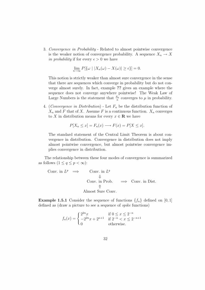
Example 1.5.1 Consider the sequence of functions fn defined on [0, 1]defined as (draw a picture to see a sequence of spike functions)

fn(x) =

22nx if 0 ≤ x ≤ 2−n

−22nx+ 2n+1 if 2−n < x ≤ 2−n+1

0 otherwise.

32

It is clear that ∫ 1

fn(x)dx = 1,

and the sequence fn converges to the zero function everywhere on [0, 1].Therefore

limn→∞

∫ 1

fn(x)dx 6=

∫ 1

lim

n→∞fn(x)dx.

This is obviously an undesirable situation which should be avoided sincewhen dealing with limiting values we want the integrals (e.g. expectations)to converge to the right values. The assumption of uniform integrability(described below) eliminates cases like this when we cannot interchange limitand integral. It will be immediate that the uniform integrability condition isnot satisfied for the sequence fn. ♠

Let Xl on Ω be a sequence of random variables on Ω. For every c let Ωl;c

be the set points where |Xl| > c and χl;c be the indicator function of the setΩl;c. The sequence Ωl is called uniformly integrable if

limc→∞

supl

E[Xlχl;c] = 0.

It is clear that the sequence in example 1.5.1 is not uniformly integrable.

Example 1.5.2 We construct an example of a sequence of functions fnproves that convergene in probability is strictly weaker than convergencealmost surely, and convergence in Lp does not imply convergence almostsurely. We let Ω = [0, 1]. We describe the definition of fn algorithmicallyrather by a formula since it is easier to understand them in this manner.Let f ≡ 1. Define f1 and f2 by subdividing [0, 1] into [0, 1

2) and [1

2, 1] and

defining

f1(x) =

1, if x ∈ [0, 1

2);

0, otherwise., f2(x) =

1, if x ∈ [1

2, 1];

0, otherwise.

Next we consider the subdivision

[0, 1] = [0,1

3) ∪ [

1

3,2

3) ∪ [

2

3, 1],

33

and define f3, f4 and f5 to be 1 on [0, 13), [1

3, 2

3) and [2

3, 1] and 0 elsewhere.

Thus having defined fj for j < n(n+12

we look at the subdivision

[0, 1] = [0,1

n+ 1) ∪ [

1

n+ 1,

2

n+ 1) ∪ · · · ∪ [

n

n+ 1, 1]

and define fk+

n(n+12

, for k = 0, 1, · · · , n, to be 1 on [k, k+1n+1

) and 0 elsewhere. It

is immediate that the sequence fn converges to the 0 function in probabilityand in L1, however, it does not converge to 0 anywhere! Therefore conver-gence in probability is strictly weaker than almost sure convergence. Whilefn does not converge to 0 anywhere, a subsequence of it will converge almostsurely to the 0 function. This is a general phenomenon, i.e., convergence inL1 implies that a subsequence converges almost surely. ♠

The most important facts about convergence of sequences of functionscan be summarized as follows:

Theorem 1.5.1 Let fn be a sequence of integrable functions

1. If fn are non-negative, then∫Ω

lim inf fn ≤ lim inf∫Ωfn.

2. If the sequence fn is monotone in the sense that fn(ω) ≤ fn+1(ω) (al-most surely) for all ω ∈ Ω and all n, then

limn

∫Ωfndµ =

∫Ω(lim fn)dµ,

where both sides of the equation are allowed to be ∞.

3. Assume there is an integrable function g such that |fn(ω)| ≤ g(ω) (al-most surely) for all ω ∈ Ω. Then

limn

∫Ωfndµ =

∫Ω(lim fn)dµ.

The same conclusion hold if the sequence is uniformly integrable.

34

We had noted earlier that even when the distribution function F of arandom variable is not differentiable, it is possible to make sense out of dFby for example assigning the value F (b) − F (a) to an interval I = [a, b] ormore precisely by defining∫

χI(x)dF (x) = F (b)− F (a).

This means that while dF may not make sense as a function, it is meaningfulas a measure µ assigning the value µ(I) = F (b) − F (a) to the interval I =[a, b]. For this measure space (R,A, µ), A is the family of subsets of Rwhich can be written as countable unions and/or intersections of intervals(open,closed or half closed). It is customary to refer to this A as the familyof Borel sets in R.

It is useful to cast our previous considerations on infinite visits to a tran-sient state and infinite appearance of a pattern in a more measure theoreticframework. This requires no new ideas and we will repeat the same argu-ments. The general question can be formulated as follows: Suppose we havean infinite sequence of events Al, then what is the probability that infinitelymany of Al’s occur? The event that infinitely many of Al’s occur is repre-sented as

A =⋂l

∞⋃m=l

Am. (1.5.1)

Lemma 1.5.1 With the above notation and hypotheses

1. P [A] = 0 if∑P [Al] <∞.

2. P [A] = 1 if∑P [Al]1∞ and A1, A2, . . . are independent.

Proof - Since A ⊂ ∪∞m=lAm

P [A] ≤∞∑

l=m

P [Am] −→ 0

which proves the first assertion. To prove the second assertion let A′ =∪l ∩∞m=l A

′m denote the complement of A. Then

P [∩∞m=lA′m] = lim

N→∞P [∩∞m=lA

′m]

(by independence) =∏

(1− P [Am])

≤∏e−P [Am]

= exp(−∑

P [Am]) = 0,

35

proving the lemma. ♣

36

EXERCISES

Exercise 1.5.1 A computer is generating )’s and 1’s with probabilities p and1− p. Let Al be the event that there is sequence of length l of 0’s in the timeperiod 2l, 2l + 1, . . . , 2l+1. Show that

P [Al infinitely often] =

1, if p ≥ 1

2;

0, otherwise.

(Hint - Let B(l)i be the event that there is a sequence of l consecutive 0’s

beginning at time 2l + (i− 1)l.)

37