1 ten deadly statistical traps in pharmaceutical quality control lynn torbeck pharmaceutical...
TRANSCRIPT
1
Ten Deadly Statistical Traps in Pharmaceutical Quality Control
Lynn Torbeck
Pharmaceutical Technology
29 March 2007

2
Your Morning Mantra
“In theory there is no difference between
theory and practice, but in practice there is.”
Yogi Berria
3
The Ten Deadly Sins
1. Graphs
2. Normal Distribution
3. Statistical Significance
4. Xbar 3S
5. %RSD
4
The Ten Deadly Sins
6. Control Charts
7. Setting Specifications
8. Cause and Effect
9. Variability
10. Sampling Plans
5
Graph? What &%$# Graph?
Q#1 “Have you graphed the data?” I have solved many statistical problems by
simply graphing the data.Always, always, always plot your data.No ink on the page that isn’t needed.Cause and effect on the same page.Make the answer appear obvious.Read Edward Tufte’s books
6
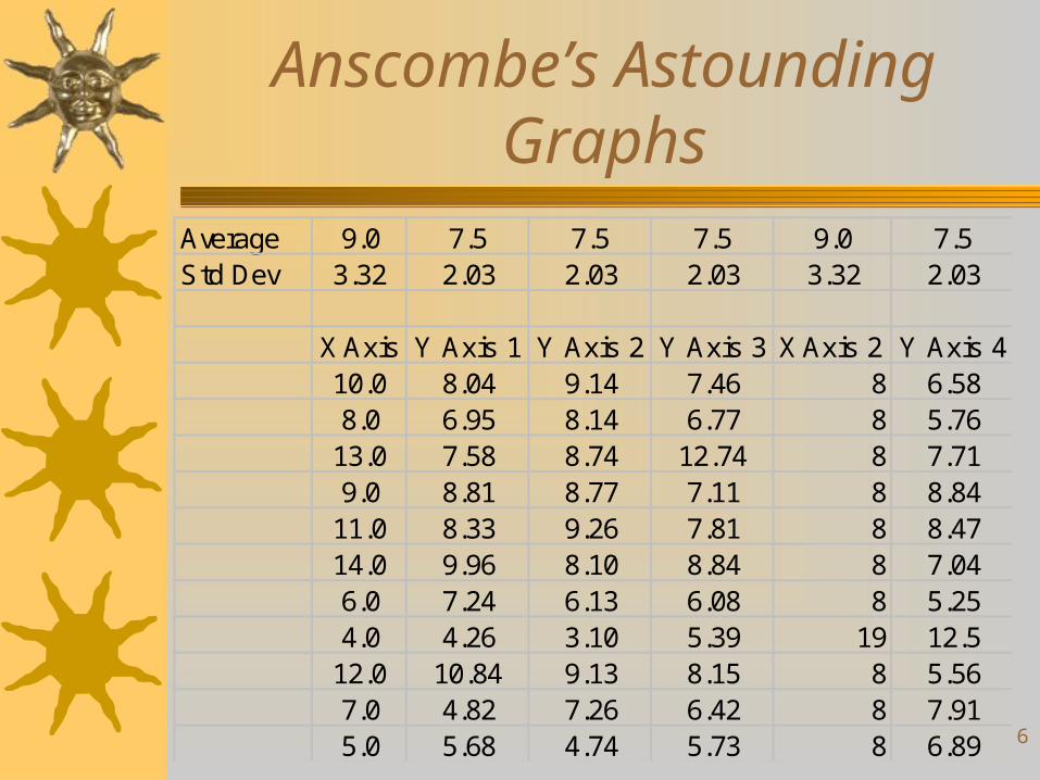
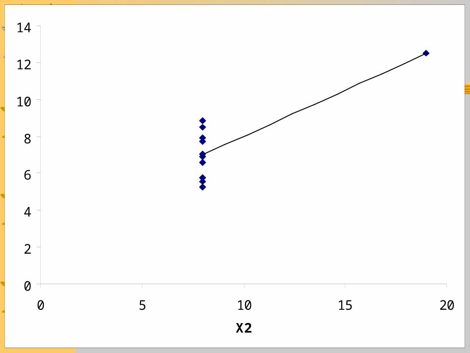
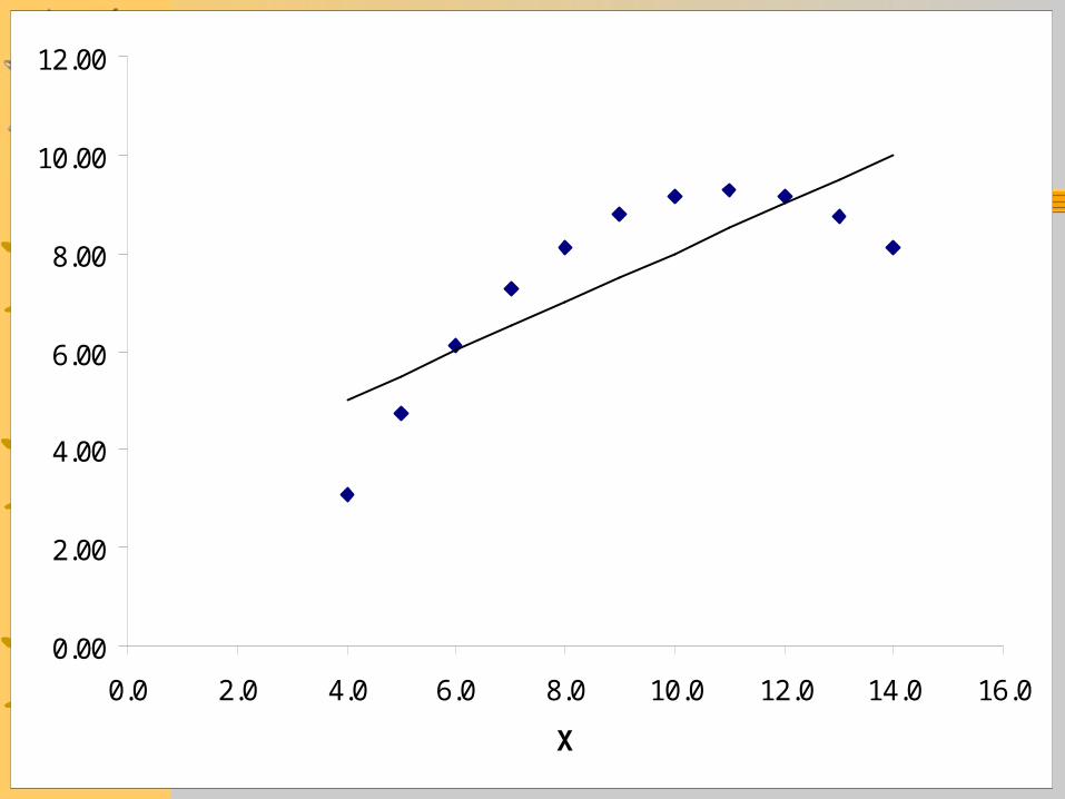
Anscombe’s Astounding Graphs
Average 9.0 7.5 7.5 7.5 9.0 7.5Std Dev 3.32 2.03 2.03 2.03 3.32 2.03
X Axis Y Axis 1 Y Axis 2 Y Axis 3 X Axis 2 Y Axis 410.0 8.04 9.14 7.46 8 6.588.0 6.95 8.14 6.77 8 5.76
13.0 7.58 8.74 12.74 8 7.719.0 8.81 8.77 7.11 8 8.84
11.0 8.33 9.26 7.81 8 8.4714.0 9.96 8.10 8.84 8 7.046.0 7.24 6.13 6.08 8 5.254.0 4.26 3.10 5.39 19 12.5
12.0 10.84 9.13 8.15 8 5.567.0 4.82 7.26 6.42 8 7.915.0 5.68 4.74 5.73 8 6.89
7
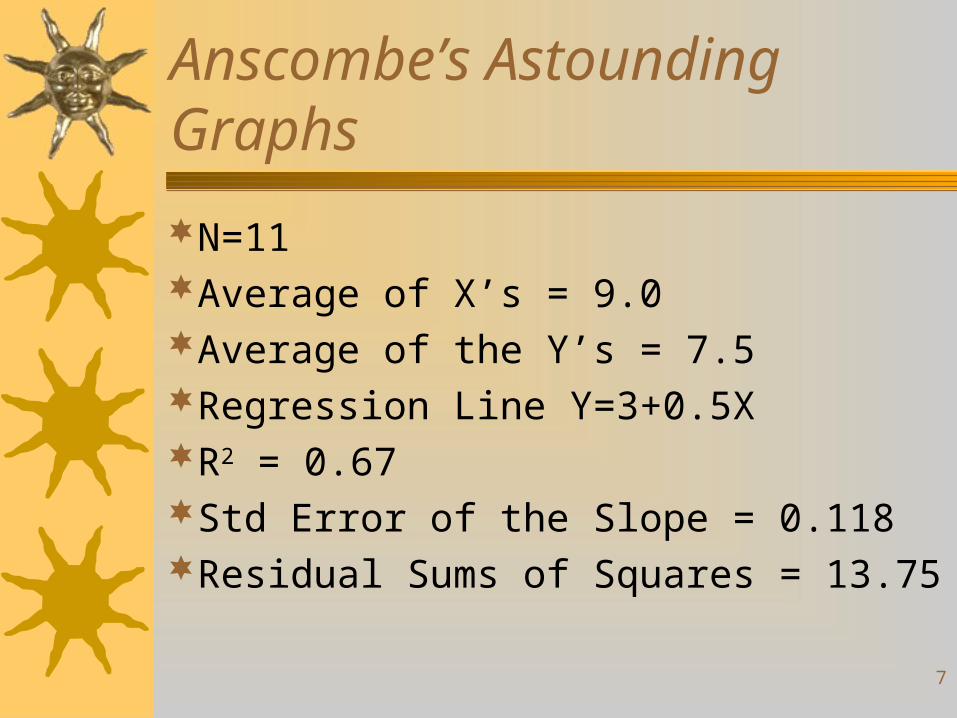
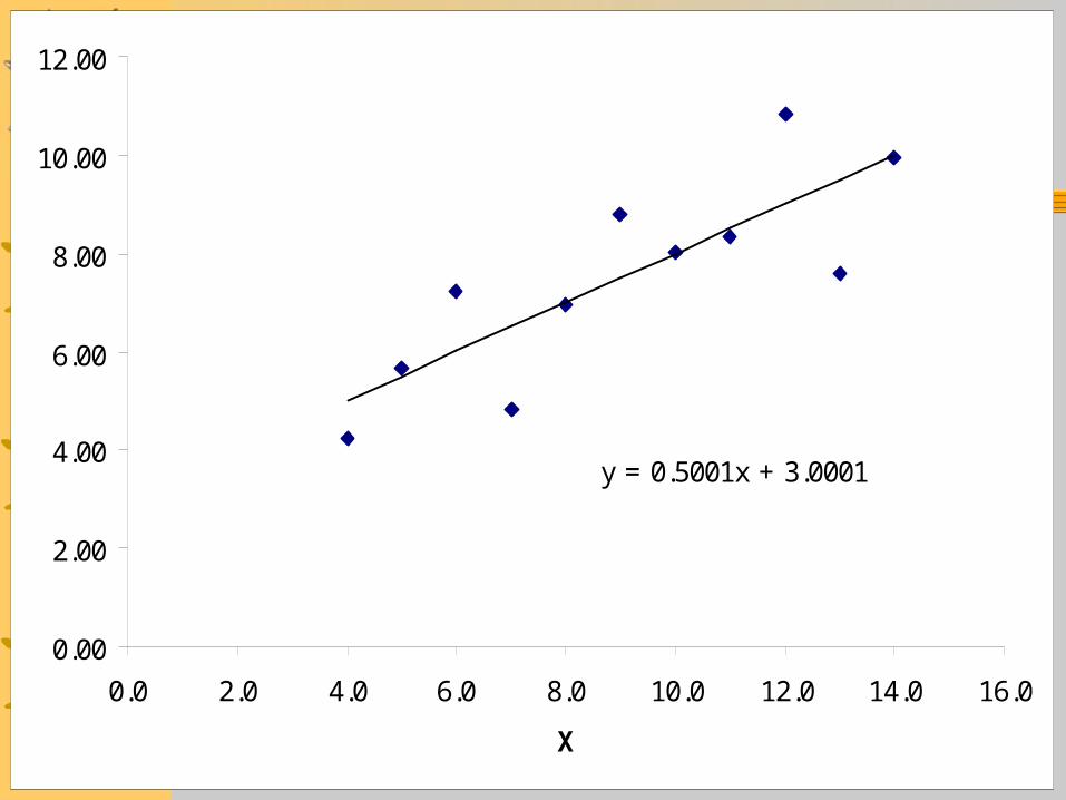
Anscombe’s Astounding Graphs
N=11Average of X’s = 9.0Average of the Y’s = 7.5Regression Line Y=3+0.5XR2 = 0.67Std Error of the Slope = 0.118Residual Sums of Squares = 13.75
8
y = 0.5001x + 3.0001
0.00
2.00
4.00
6.00
8.00
10.00
12.00
0.0 2.0 4.0 6.0 8.0 10.0 12.0 14.0 16.0
X
9
0.00
2.00
4.00
6.00
8.00
10.00
12.00
14.00
0.0 2.0 4.0 6.0 8.0 10.0 12.0 14.0 16.0
X
10
0
2
4
6
8
10
12
14
0 5 10 15 20
X2
11
0.00
2.00
4.00
6.00
8.00
10.00
12.00
0.0 2.0 4.0 6.0 8.0 10.0 12.0 14.0 16.0
X
12
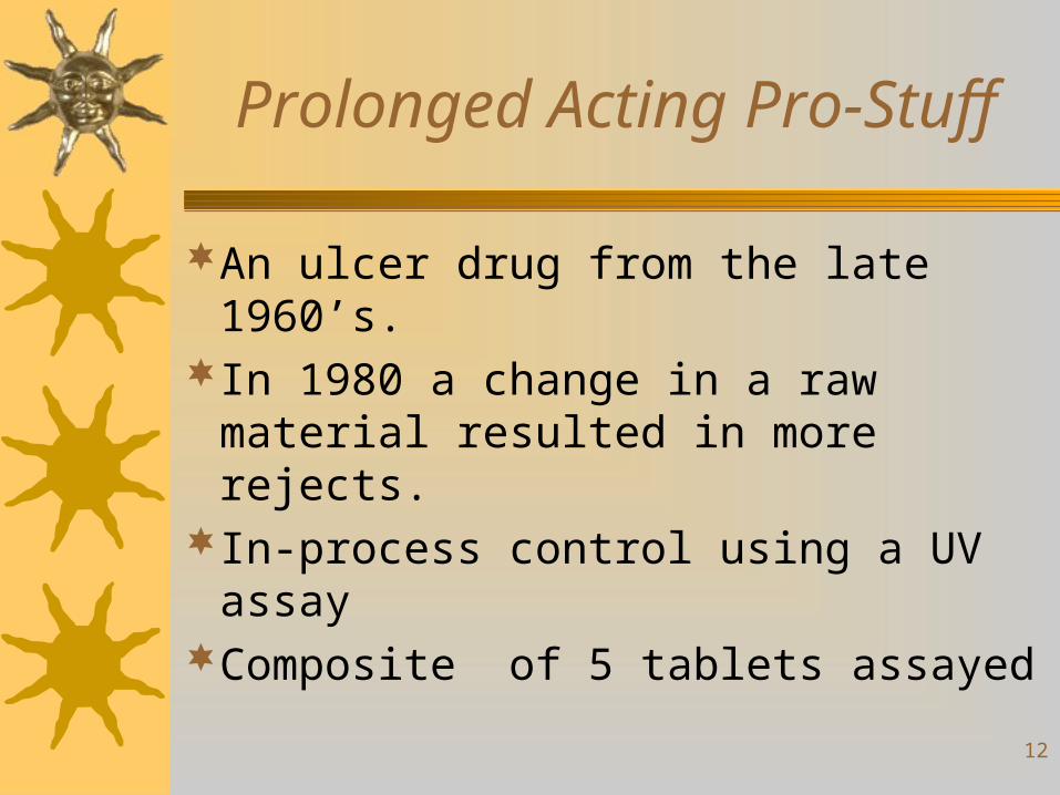
Prolonged Acting Pro-Stuff
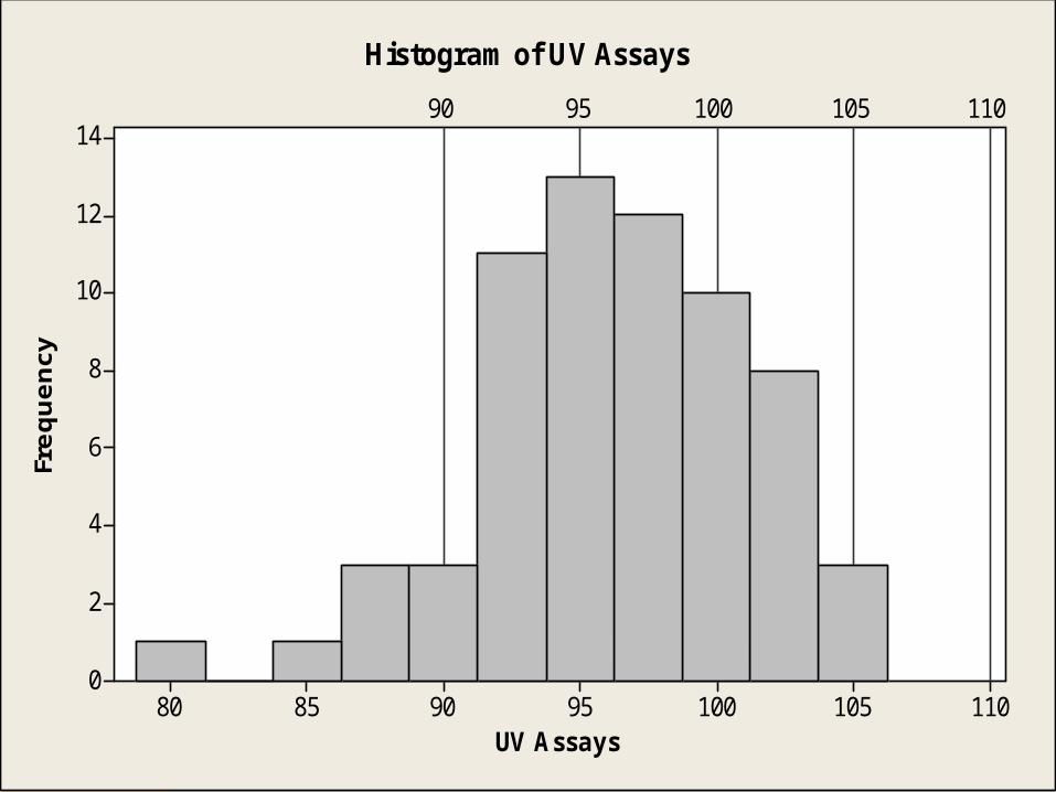
An ulcer drug from the late 1960’s.In 1980 a change in a raw material resulted
in more rejects.In-process control using a UV assayComposite of 5 tablets assayed
13
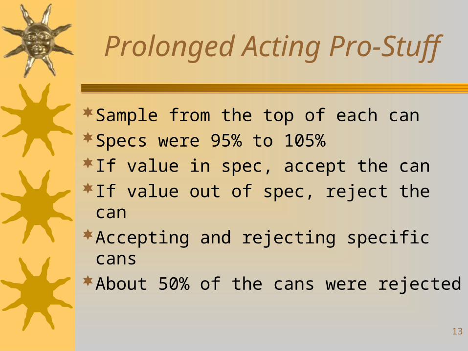
Prolonged Acting Pro-Stuff
Sample from the top of each canSpecs were 95% to 105%If value in spec, accept the canIf value out of spec, reject the canAccepting and rejecting specific cansAbout 50% of the cans were rejected
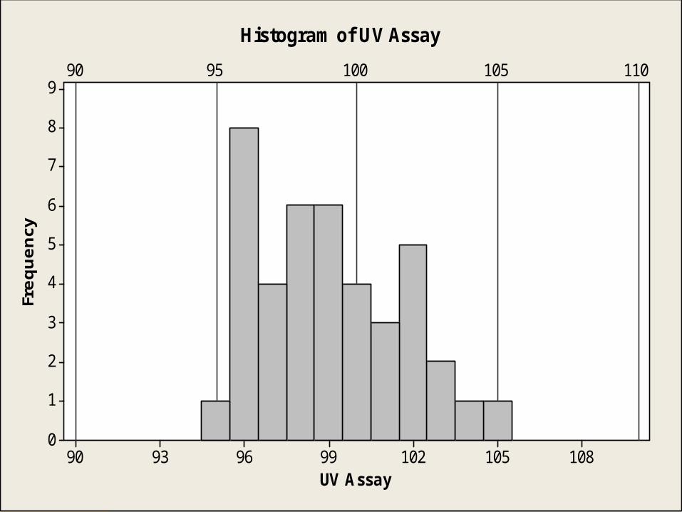
14UV Assay
Frequency
10810510299969390
9
8
7
6
5
4
3
2
1
0
90 95 100 105 110
Histogram of UV Assay
15UV Assays
Frequency
11010510095908580
14
12
10
8
6
4
2
0
90 95 100 105 110
Histogram of UV Assays
16Retests
Frequency
108104100969288
3.0
2.5
2.0
1.5
1.0
0.5
0.0
90 95 100 105 110
Histogram of Retests
17
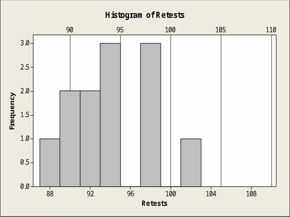
Prolonged Acting Pro-Stuff
No good cans or bad cans.Some “good” cans when retested are now
out of specifications.The cans accepted are just as bad or good
as the cans rejected.45% of the values are OOSThe product was taken off the market.A personal story
18
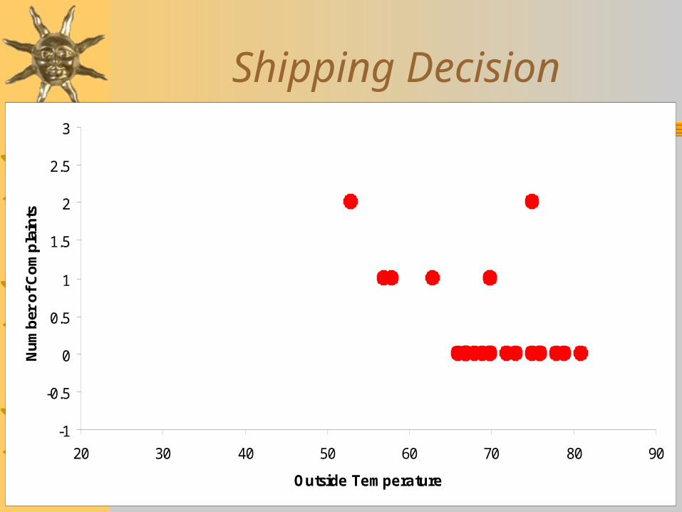
Shipping Decision
-1
-0.5
0
0.5
1
1.5
2
2.5
3
20 30 40 50 60 70 80 90
Outside Temperature
Nu
mb
er o
f C
om
pla
ints
19
A Little Normal History
The concept of the Normal is basic.Also called Gaussian or Bell Curve.First published in November 12, 1733.First set of tables in 1799 !Used by the astronomer Laplace for errors.First called the Normal in 1893 by the
statistician Karl Pearson.
20
They Were Blown Away
“I know of scare anything so apt to impress the imagination as the wonderful form of cosmic order expressed by the ‘Law of Frequency of Error.’”
Francis Galton in Natural Inherence, 1888
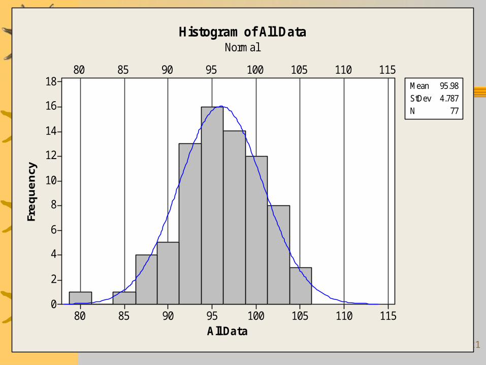
21All Data
Frequency
11511010510095908580
18
16
14
12
10
8
6
4
2
0
80 85 90 95 100 105 110 115Mean 95.98StDev 4.787N 77
Histogram of All DataNormal
22
Hunting the Elusive Normal
I have never met a real Normal distribution. Gotten close a couple of times.
There are no real Normal distributionsIt’s a theoretical fiction that is useful part
of the time.We must separate reality from theory.
23
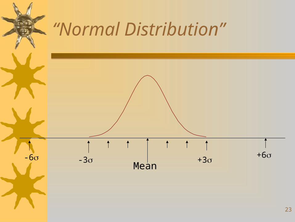
“Normal Distribution”
Mean+3 +6
-3-6
24
Normal Facts
In theory, the tails of the distribution stretch from minus infinity to plus infinity, but there are real physical limits.
It is unique in that it is fully described by just its mean, mu, , and its standard deviations, sigma, , which are almost never actually known for certain.
Probabilities are represented by areas.
25
What’s Normally Normal?
Tablet and capsule weightsMost manufactured partsStudent test scores, the ‘bell curve’ againThings that grow in nature:
– Apples– Bird eggs– Flowers– Peoples heights
26
Ain’t Never Gonna be Normal
Particle sizesLAL, EU/mLBioburden, cfu/mLFailures of most anythingTelephone calls per unit of timeChurch contributionsFloods
27
Watch Out!
The tails are the most volatile and unstableBut, that is often the area of most interest!Difficult to tell if data are normally
distributed by looking at a small sample.Crude rule is that we need at least 100
representative data values to determine if it is even approximately normal.
28
Statistical Significance:Who Cares ?
The role of statistical analysis is as an additional tool to assist the scientist in making scientific interpretations and conclusions and not an end in itself.
29
Differences
A scientific analysis often takes the form of looking for significant differences.
Is drug A different from drug B?Is the increase in yield significantly better
with the new centrifuge?A difference can be significant in two
ways, practical and statistical.
30
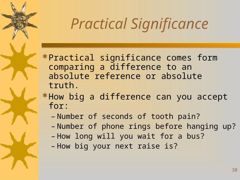
Practical Significance
Practical significance comes form comparing a difference to an absolute reference or absolute truth.
How big a difference can you accept for:– Number of seconds of tooth pain?– Number of phone rings before hanging up?– How long will you wait for a bus?– How big your next raise is?
31
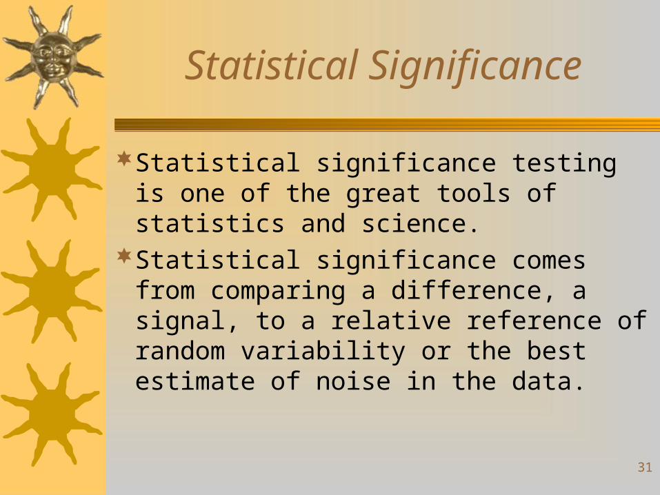
Statistical Significance
Statistical significance testing is one of the great tools of statistics and science.
Statistical significance comes from comparing a difference, a signal, to a relative reference of random variability or the best estimate of noise in the data.
32
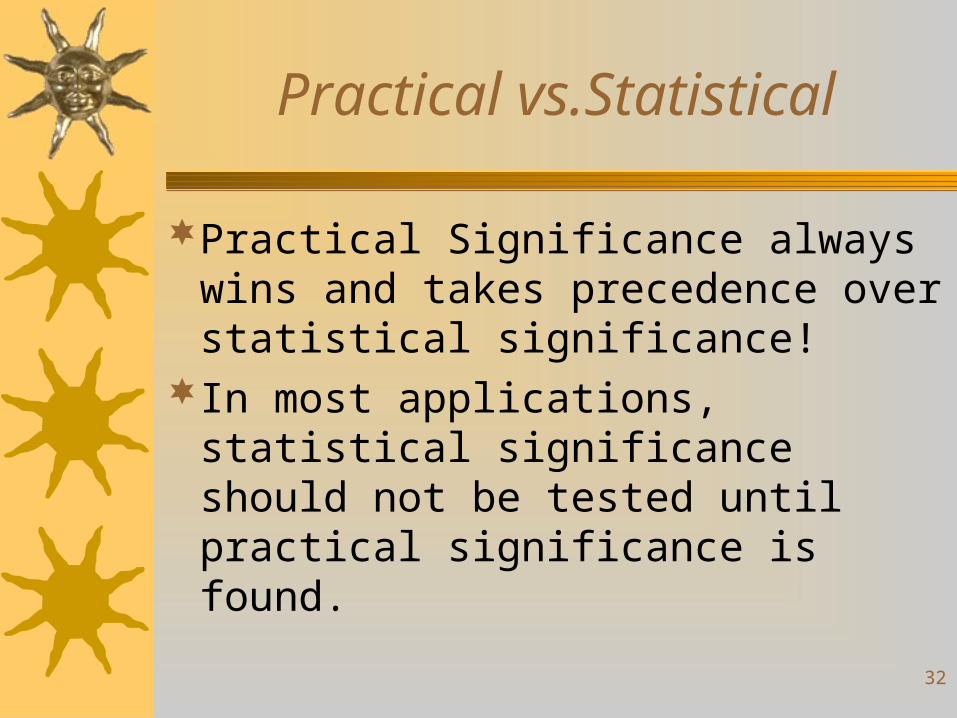
Practical vs.Statistical
Practical Significance always wins and takes precedence over statistical significance!
In most applications, statistical significance should not be tested until practical significance is found.
33
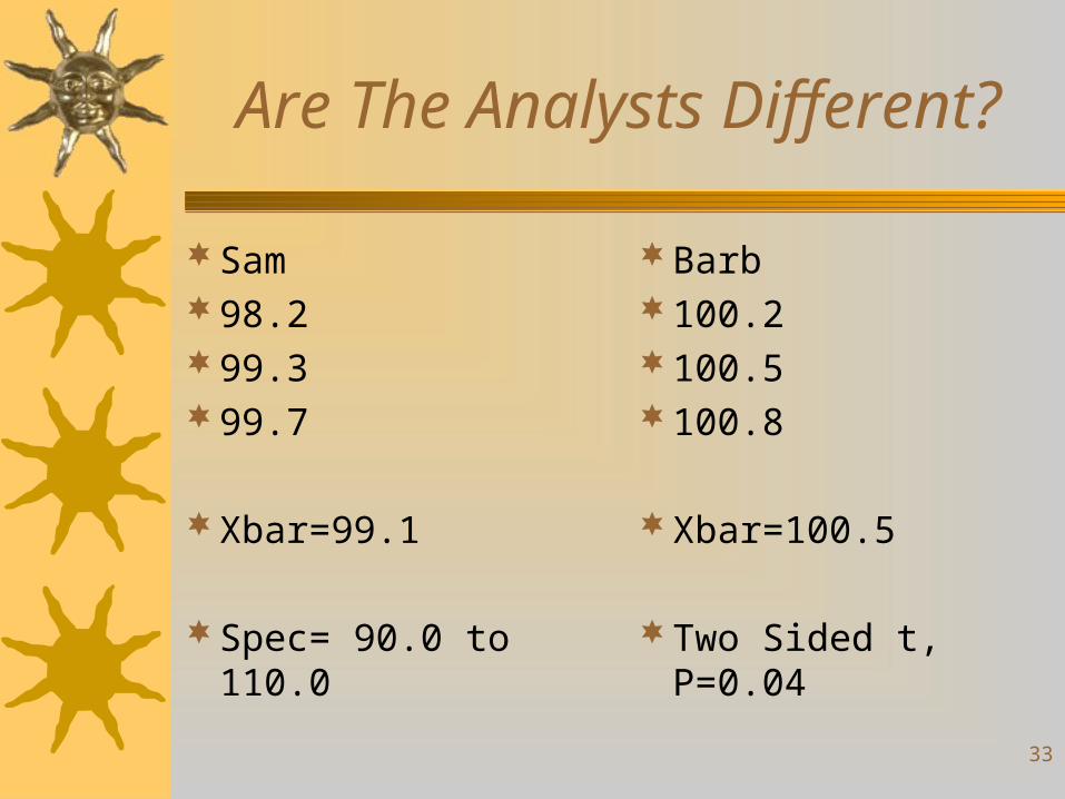
Are The Analysts Different?
Sam98.299.399.7
Xbar=99.1
Spec= 90.0 to 110.0
Barb100.2100.5100.8
Xbar=100.5
Two Sided t, P=0.04
34
Signal to Noise
All statistical significance testing is only a comparison of the signal to the noise.
If the signal can be shown to be larger than the noise, than we would expect by chance variation alone, we say it is significant.
Bigger signal more significant.Smaller noise more significant.
35
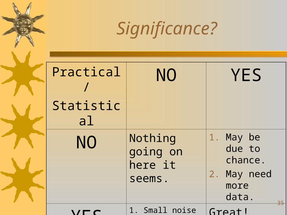
Significance?
Practical /
StatisticalNO YES
NO Nothing going on here it seems.
1. May be due to chance.
2. May need more data.
YES 1. Small noise
2. Large sample size.
What does it mean?
Great! Everybody is happy.
36
Why Do It To It?
The primary purpose of statistical tests of significance is to prevent a us from accepting an apparent result as real when it could be just due to random chance.
Statistical significance without practical significance could in some circumstances be a lead to finding new relationships.
What if the spec was changed to 98.0 to 102.0?We may want to find out why different
37
The Biggest Lie in Statistics?
Your statistics professor mislead or lied.Is Xbar±3S ever Correct?For ever complex problem there is a
solution that is quick, simple, understandable and absolutely wrong!
More grief has been perpetuated by this formula than any in statistics.
38
The Biggest Lie in Statistics?
What is true is that 3 will bracket 99.73% of the area under the normal cures.
Note that this assumes we know the true values for the mean mu, , and standard deviation, sigma, , which we never do of course. We have to estimate them with the small samples we take.
Thus, there is uncertainty in the estimates.
39
Side Line
Did you hear about the statistician’s wife who said her husband was just average?
She was being mean.
40
So, What Do I Do Now?
Don’t use Xbar±3S as generalized monkey wrench and apply it to all of your statistical questions. Use the right tool for the job.
Use Confidence Intervals to bracket the unknown mean.
Use Tolerance Intervals to bracket a given percentage of the individual data values.
41
%RSD: Friend or Foe?
S= SQRT[(X-Xbar)2/(n-1)]%RSD = (100 * S) / XbarThey are two different summary statisticsThey measure two different conceptsThey are not substitutes for each otherWe need to report both.
42
Control Charts
Having just told you not to use Xbar±3S, I now have to tell you that is how control charts define the control limits.
This is an artifact of history.Control charts were developed by Dr.
Walter Shewhart in 1924 while working at Western Electric in Cicero Ill.
43
Control Chart
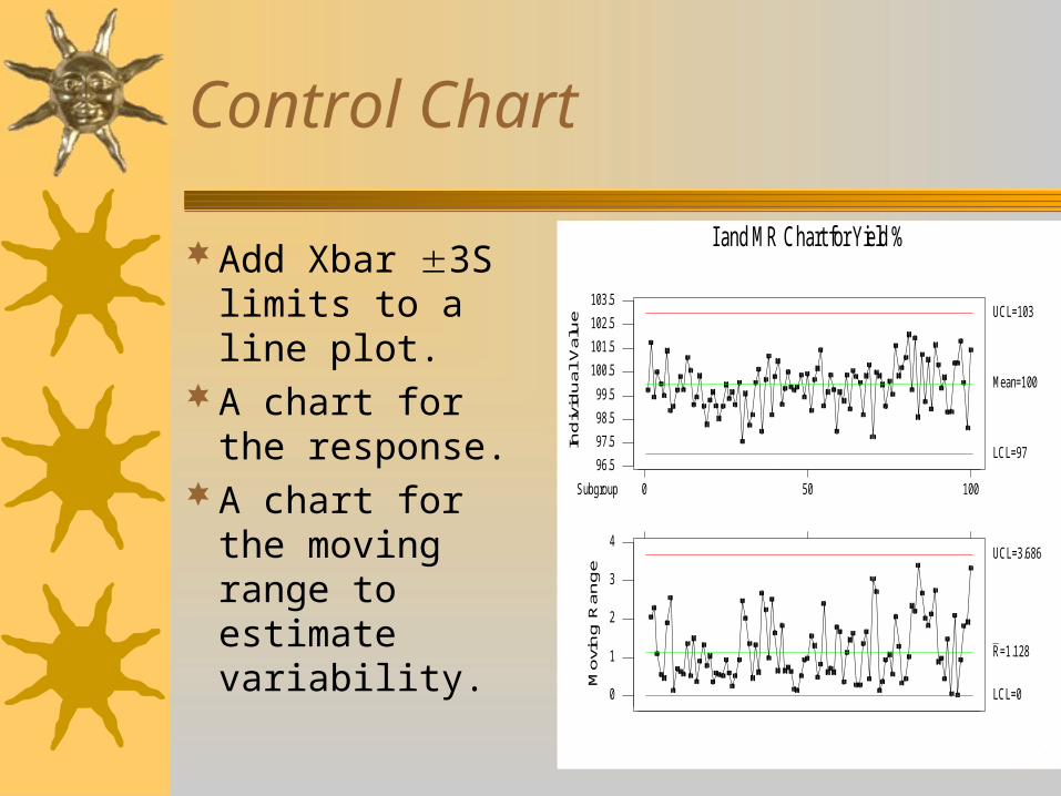
Add Xbar 3S limits to a line plot.
A chart for the response.
A chart for the moving range to estimate variability.
0Subgroup 50 100
96.5
97.5
98.5
99.5
100.5
101.5
102.5
103.5
Ind
ivid
ual
Val
ue
Mean=100
UCL=103
LCL=97
0
1
2
3
4
Mov
ing
Ran
ge
R=1.128
UCL=3.686
LCL=0
I and MR Chart for Yield %
44
Do You Trust YourControl Chart?
Control charts are crude tools and not exact probability statements.
They don’t take into account the number of samples in the data set for the limits.
They are intended as early warning devices and not accept/reject decision tools.
Don’t use for large $$ decisions.
45
Oh Wow, I Don’t Believe It !
You did what to set the specification criteria for
your million dollar product?
46
Setting Specifications
A specification is a document that contains methods and accept/reject criteria
Criteria can be determined several ways– Wishful thinking– Clinical results– Compendial standards– Historical data and statistics
47
Million $$ Decisions?
Regulatory Limits - ExternalRelease: accept/reject - InternalAction limitsAlert
– Warning limits– Trend limits– Validation limits
48
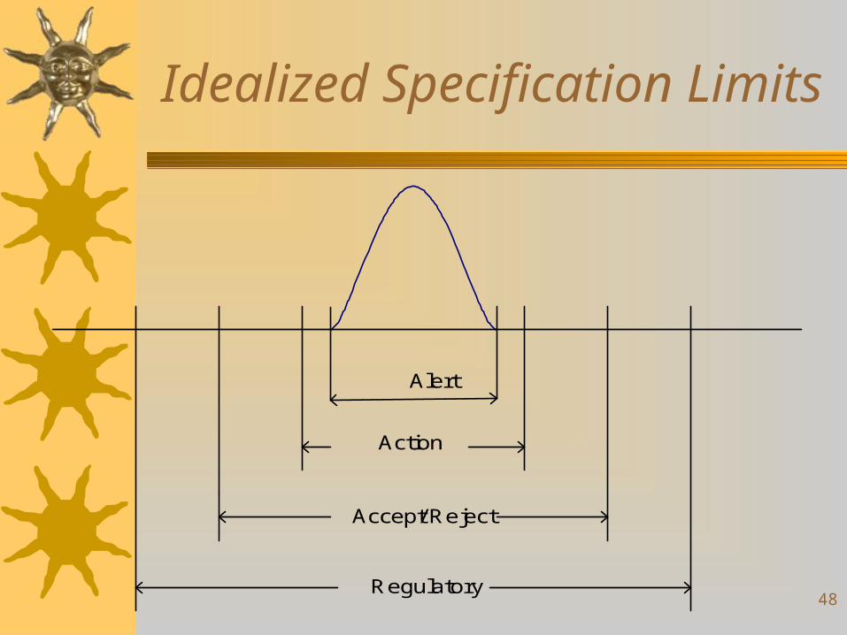
Idealized Specification Limits
Accept/ Reject
Regulatory
Alert
Action
49
Calculating Criteria
Don’t use Confidence Intervals, they shrink toward zero with large sample sizes.
Don’t use X bar ± 3 S. They are too narrow for small sample sizes
Use Tolerance Intervals, preferably 99%/99%. This will take into consideration the sample size and uncertainty of the average and the standard deviation.
50
Setting Specification Criteria
For action limits, expect the average to vary and widen the Tolerance Limits
For accept/reject limits, add a further allowance for stability.
Consider the clinical results when possible as part of the justification for limits.
51
Drunken Teachers
Did you know that there is a positive correlation between alcohol consumption and High School teacher’s salaries?
That there is a negative correlation between average student’s test scores for a state and the distance of the state capital from the Canadian boarder?
52
Cow Magnets Cure Gout
What’s a cow magnet?What is gout?How do we test a cause and effect
relationship to see if this works?Should we just ask people what they think?“No causation without manipulation.”Gold Standard is double blind clinical trial.
53
Variability is the Enemy
How many OOS values were documented in the lab last year?
How many manufacturing deviations were investigated last year?
How many lots were rejected last year?How many of your quality problems would
go away if there were no variation?
54
Misconceptions of variability
We have variability because the equipment needs to be replaced with new technology.
We do too many tests.Variability exists because some idiot didn’t
do their job correctly. Variability is an inherent fact of life and
there isn’t a darn thing we can do about it except to live with it. It’s cost of business.
55
Variability is the Enemy
“Special Cause” variation is the result of a single source. Use CAPA to solve it.
“Common Cause” variation is the result of multiple small sources all contributing to the sum total.
CAPA will not work for common causeWe need a culture change to address
common cause variation
56
Sources of Variation:
Common cause variation:– People– Materials– Methods– Measurement– Machines– Environment
57
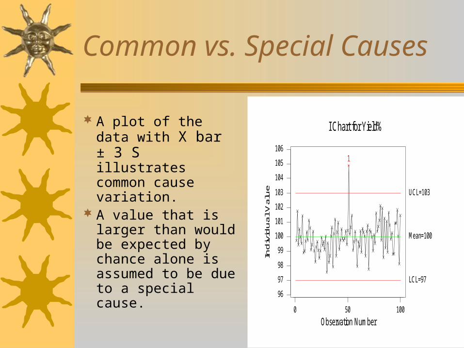
Common vs. Special Causes
A plot of the data with X bar ± 3 S illustrates common cause variation.
A value that is larger than would be expected by chance alone is assumed to be due to a special cause.
0 50 100
96
97
98
99
100
101
102
103
104
105
106
Observation Number
Ind
ivid
ual
Val
ue
I Chart for Yield%
1
Mean=100
UCL=103
LCL=97
58
Deming’s Message
Dr. W. Edwards Deming was the very famous statistician that taught statistical quality control to the Japanese in the 50’s.
“If I had to reduce my message for management to just a few words, I’d say it all had to do with reducing variation.”
59
Deming’s Message
If you reduce variability, you will reduce scrap, rejects and rework. You can then make a better product at less cost. You will capture a larger market share. Your people will be employed and you will prosper.
• Paraphrase of Deming’s message
60
Confronting the Enemy
Operational DefinitionsAchieve the TargetFlexible ConsistencyHold Constant Controllable FactorsMistake ProofingNew TechnologyContinuous and forever improvement
61
The Black Hole of Quality
Like a black hole with light, sampling plans just suck the common sense right out of people’s brains.
Normal, logical and rational people suddenly become willfully and terminally stupid.
Many myths and misconceptions about what sampling plans can and can not do.
62
Black Hole Facts
A sample is only a small part of the wholeEach sample is going to be differentSome samples will have many defectsSome samples will have few defectsBigger sample, better estimate.On average, the defect percent can only be
estimated and not known perfectly.
63
Black Hole Facts
There is a small but real probability that a good lot of product will be rejected.
Called the “Producer’s Risk, usually 5%.There is a small but real probability that a
bad lot will be accepted.“Consumer’s Risk, usually 5% or 10%Most common plan is ANSI/ASQ Z1.4.
64
Black Hole Facts
“The AQL is the quality level that is the worst tolerable process average … .”
“The acceptance of a lot is not intended to provide information about lot quality.”
“The standard is not intended as a procedure for estimating lot quality or for segregating lots.”
65
Black Hole Facts
“The purpose of this standard is, through the economic and psychological pressure of lot non-acceptance, to induce a supplier to maintain a process average at least as good as the specified AQL while at the same time providing an upper limit on the consideration of the consumer’s risk of accepting occasional poor lots.”
66
Misunderstandings
Double and multiple sampling plans are not testing into compliance.
It is not possible to have an AQL=0.0Accept on zero, reject on one is not always
the best plan for critical defects.If the lot size is ten times or more than the
sample size, then the lot size doesn’t matter.
67
Summary
“Statistical thinking will one day be as necessary for efficient citizenship as the ability to read and write.”
H. G. Wells
68
References
NIST online statistics textbook– http://www.itl.nist.gov/div898/handbook/
index.htm
Edward Tufte’s website– http://www.edwardtufte.com/tufte/
W. Edwards Deming’s book– Out of the Crisis
69
References
Torbeck, Lynn.,Using Statistics to Measure and Improve Quality, DHI Publishing 2004.
De Muth, James (1999). Basic Statistics and Pharmaceutical Statistical Applications, Marcel Dekker.

70
“That’s All Folks”
Thank you !Questions ?