1 the mathematical methods of electrodynamics · igor n. toptygin: foundations of classical and...
TRANSCRIPT

�
� Igor N. Toptygin: Foundations of Classical and Quantum Electrodynamics —Chap. c01 — 2013/10/8 — page 1 — le-tex
�
�
�
�
�
�
1
1The Mathematical Methods of Electrodynamics
1.1Vector and Tensor Algebra
1.1.1The Definition of a Tensor and Tensor Operations
In three-dimensional space, select a rectangular and rectilinear (Cartesian1)) systemof coordinates x1, x2, x3. Regard the space as Euclidean. This means that all axiomsof Euclidean geometry2) and their consequences considered in school courses onmathematics are valid in it. For instance, the square of the distance between twoclose points is given by the following expression:
dl2 D dx21 C dx2
2 C dx23 .
Along with the original system of coordinates, consider some other systems ofcommon origin yet rotated with respect to the original one (Figure 1.1).
Figure 1.1 The rotation of the Cartesian system of coordinates.
1) René Descartes (Renatus Cartesius)(1596–1650) was a French philosopherand mathematician, the founder of thecoordinates method. He introduced a largenumber of mathematical concepts andnotations used even now.
2) Euclid (lived in the third century BC) wasan ancient Greek scientist, “the father ofgeometry.” His mathematical treatise entitledElements is the best known. Euclid studiedvarious aspects of geometric optics.
Foundations of Classical and Quantum Electrodynamics, First Edition. Igor N. Toptygin.©2014 WILEY-VCH Verlag GmbH & Co. KGaA. Published 2014 by WILEY-VCH Verlag GmbH & Co. KGaA.

�
� Igor N. Toptygin: Foundations of Classical and Quantum Electrodynamics —Chap. c01 — 2013/10/8 — page 2 — le-tex
�
�
�
�
�
�
2 1 The Mathematical Methods of Electrodynamics
A scalar or invariant is a quantity that does not change when the system of coor-dinates is rotated, that is, it is the same in either the original or the rotated systemof coordinates
S 0 D S D inv . (1.1)
For instance, dl2 D dl 02 D inv.In three-dimensional space, a vector is the titality of three quantities Vα (α D
1, 2, 3) defined in all coordinate systems and transformed according to the follow-ing rule:
V 0α D aα�V� (1.2)
(summing of elements over the repeated symbol �, from 1 to 3 is assumed). HereV� are the projections of the vector on an axis of the original system of coordinates,V 0
α are the projections of the vector on an axis of the rotated system, and aα� arethe coefficients of the transformation, which are the cosines of the angles betweenthe � axis of the original system and the α axis of the rotated system. They may bewritten through the single vectors (orts) of the coordinate axes:
aα� D e0α � e� . (1.3)
In three-dimensional space, a tensor of rank 2 is a nine-component quantity Tα�
(each index varies independently assuming three values: 1, 2, 3) which is definedin every system of coordinates and, when a coordinate system is rotated, is trans-formed as the products of the components of the two vectors A αV� , in the follow-ing way:
T 0α� D aαμ a�ν Tμν . (1.4)
In three-dimensional space, a tensor of rank s is a 3s-component quantity Tλ...ν
that is transformed as the product of s components of vectors:
T 0�...� D a�μ . . . a�σ Tμ...σ . (1.5)
Scalars and vectors may be regarded as tensors of rank 0 and 1, respectively.Rotation matrixba has the following properties:
1. Orthogonality
aαμ a�μ D δα� , aαμ aαν D δμν , (1.6)
where
δα� D 1 if α D � and δα� D 0 if α ¤ � (1.7)
is Kronecker symbol3);
3) Leopold Kronecker (1823–1891) was a German mathematician, a specialist in algebra and theoryof numbers.

�
� Igor N. Toptygin: Foundations of Classical and Quantum Electrodynamics —Chap. c01 — 2013/10/8 — page 3 — le-tex
�
�
�
�
�
�
1.1 Vector and Tensor Algebra 3
2. The determinant of a rotation matrix equals 1:
detba � jbaj D 1 . (1.8)
3. The product of two rotation matrices
bc Dbabg , cα� D aαμ gμ� (1.9)
describes the evolution of a system resulting from two consecutive rotations,first with matrixbg and then with matrixba.4) In the general case, rotation matri-ces are noncommutative, that is,
babg ¤bgba . (1.10)
As follows from property 1, a reverse matrix defined by the relation
ba�1ba Dbaba�1 Db1 or a�1αμ aμ� D aαμ a�1
μ� D δα (1.11)
results from the original matrix when the latter is transposed, that is, itscolumns are substituted for lines and vice versa:
ba�1 DbQa , a�1α� D Qaα� D a�α . (1.12)
The reverse transformation (1.2) looks like this:
V� D a�1�α V 0
α . (1.13)
All vectors are transformed identically according to rule (1.2) when a coordinatesystem is rotated. But they may behave in one of two ways if a system of coordinatesis inverted, that is,
x 0α D �xα . (1.14)
Here the transformation matrix is aα� D �δα�. Vectors whose components, justlike coordinates xa , change their signs during inversions are called polar (regu-lar, real) vectors. Vectors whose components do not change sign as the result ofinversions of coordinate systems are called axial vectors or pseudovectors (an angu-lar velocity, a cross-product of two polar vectors A � B, etc.) This definition alsoincludes tensors of arbitrary rank s: when the inversion of coordinates occurs, thecomponents of polar (regular) tensors acquire a factor of (�1)s and the componentsof pseudotensors acquire a factor of (�1)sC1.
The sum of two tensors of the same rank produces a third tensor of the samerank with components
Q α� D Tα� C Pα� . (1.15)
4) The family all rotation operations forms makes a group of three-dimensional rotations.See Gel’fand et al. (1958).
�
� Igor N. Toptygin: Foundations of Classical and Quantum Electrodynamics —Chap. c01 — 2013/10/8 — page 4 — le-tex
�
�
�
�
�
�
4 1 The Mathematical Methods of Electrodynamics
The direct products of the components of two tensors (without summing) constitutea tensor whose rank equals the sum of the ranks of the factors, for instance,
Q α�λ D Tα�Vλ , (1.16)
where Q α�λ is a tensor of rank 3.The contraction of a tensor means the formation of a new tensor whose compo-
nents are produced by the selection of components with two identical symbols and,further, their summing. For instance, Q α�� D A α is a vector and Q α�α D B� isanother vector. Contraction decreases the rank of the tensor by 2, for instance,
S D Tαα D inv (1.17)
is a scalar.When an equality between tensors is written, the rule of the same tensor dimen-
sionality must be observed: only tensors of the same rank may be equated. Thismeans that the number of free symbols (over which no summation is done) mustbe the same in the first and second members of an equality. The number of pairsof “mute” symbols (those over which summing is done) may be any on the rightand on the left.
Tensors may be symmetric (antisymmetric) with respect to a pair of indices αand � if their components satisfy the conditions
Q α�μ D Q �αμ (Q α�μ D �Q �αμ) . (1.18)
Tensor components may be either real or complex numbers. In the latter case, theconcepts of Hermitian5) and anti-Hermitian tensors play an important role. Thedefinition of a Hermitian tensor is as follows:
T hα� D T h�
�α , (1.19)
where the asterisk indicates complex conjugation. The definition of an anti-Hermitian tensor is as follows:
T ahα� D �T ah�
�α . (1.20)
In applications, invariant unit tensors δα� and eα�λ are very important. The for-mer is a symmetric polar tensor whose components coincide with the Kroneckersymbol (1.7), whereas the latter is antisymmetric over any pair of indices, and itscomponents are determined by the following conditions:
(a) e123 D 1 , eα�λ D �e�αλ D �eαλ� D eλα� D e�λα D �eλ�α . (1.21)
5) Charles Hermite (1822–1901) was a French mathematician, the author of works on classicalanalysis, algebra, and theory of numbers.
�
� Igor N. Toptygin: Foundations of Classical and Quantum Electrodynamics —Chap. c01 — 2013/10/8 — page 5 — le-tex
�
�
�
�
�
�
1.1 Vector and Tensor Algebra 5
It is called the Levi-Civita tensor.6) Both tensors, transforming during rotations ac-cording to rule (1.7), are peculiar in that their components have the same values inall coordinate systems:
δ0α� D δα� , e0
α�λ D eα�λ . (1.22)
Problems
1.1. Prove equality (1.8). What is the determinant of the transformation matrix ifrotation is accompanied by the inversion of the coordinate axes?
1.2. Prove the equalities δ0α� D δα� and e0
αμν D eαμν for an arbitrary rotation of acoordinate system.
1.3. Write down the rule of transformation for the components of a pseudoten-sor of rank s that would be valid not just for the rotation but also for the mirrorreflections of the coordinate axes.
1.4. Represent an arbitrary tensor of rank 2 Tα� as the sum of a symmetric tensor(Sα� D S�α) and an antisymmetric tensor (A α� D �A �α). Make sure that thisrepresentation is unique.
1.5. Represent an arbitrary complex tensor of rank 2 Tα� as the sum of a Hermitiantensor (S h
α� D S h��α ) and an anti-Hermitian tensor (Ah
α� D �Ah��α). Make sure that
this representation is unique.
1.6. Show that
1. the contraction of a symmetric tensor and an antisymmetric tensor equals zero:Sα� A α� D 0.
2. the contraction of two Hermitian tensors or two anti-Hermitian tensors ofrank 2 is a real number.
3. the contraction of a Hermitian tensor and an anti-Hermitian tensor of rank 2is a purely imaginary number.
1.7. Show that the symmetry of a tensor is a property that is invariant with respectto rotations, that is, a tensor that is symmetric (antisymmetric) over a pair of indicesin a certain system of reference remains symmetric (antisymmetric) over theseindices in every system rotated with respect to the original one.
1.8. Using rules (1.2)–(1.6) of tensor transformation, show that
1. A α is a vector (pseudovector) if A α Bα D inv and Bα is a vector (pseudovector).2. A α is a vector if A α D Tα� B� in any system of coordinates and Tα� is a tensor
of rank 2, and B� is a vector;3. Tαα D inv, where Tα� is a tensor of rank 2.
6) Tullio Levi-Civita (1873–1941) was an Italian mathematician who contributed to the developmentof tensor analysis.

�
� Igor N. Toptygin: Foundations of Classical and Quantum Electrodynamics —Chap. c01 — 2013/10/8 — page 6 — le-tex
�
�
�
�
�
�
6 1 The Mathematical Methods of Electrodynamics
4. εα� is a tensor of rank 2 if A α and Bα are vectors and A α D εα� B� in allsystems of coordinates. What is εα� if A α is a vector and Bα is a pseudovector?What is εα� if A α and Bα are both pseudovectors?
5. A α�λBα� is a vector if A α�λ and Bα� are tensors of ranks 3 and 2, respectively.6. Tα� Pα� is a pseudoscalar if Tα� and Pα� are a tensor and a pseudotensor of
rank 2, respectively.
1.9. Show the rule of the transformation of an aggregate of volumetric integralsTα� D R
xα x�dV in the cases of rotation and mirror reflection (xα , x� are Carte-sian coordinates).
1.10. Show that the components of an antisymmetric tensor of rank 2 A α� D�A �α (either polar or axial) may be identified by the components of a certain vectorCα (either axial or polar) because they are transformed in the same way in the caseof rotation or reflection. In this case, Cα is called the vector dual to tensor A α�.
1.11. Prove the following equalities:
[A � B]α D eα�λA � Bλ ,
[A � B] � C D eα�λ A α B� Cλ Dˇ̌̌̌ˇ̌A 1 A 2 A 3
B1 B2 B3
C1 C2 C3
ˇ̌̌̌ˇ̌ . (1.23)
How are the vector, the dual vector, and the mixed products transformed in thecases of rotation and reflection if all three vectors are polar?
1.12. Show that if the respective components of two vectors are proportional in acertain system of coordinates, then they are also proportional in any other systemof coordinates. Vectors such as these are called parallel vectors.
1.13. The area of an elementary parallelogram constructed on the small vectorsdr and dr0 is represented by vector dS directed along a normal to the plane of theparallelogram and, by the absolute value, is equal to its area. Write down dSα intensor notation.
1.14. Write down, in tensor notation, the volume dV of the elementary paral-lelepiped constructed on the small vectors dr, dr 0, dr00. How is it transformed inthe cases of rotation and reflection?
1.15. Prove the identities
(A � B) � (C � D) � (A � C )(B � D) C (A � D)(B � C ) D 0 ,
(A � B) � (C � D) C (B � C) � (A � D) C (C � A) � (B � D) D 0 ,
A � (B � C ) C B � (C � A) C C � (A � B) D 0 ,
(A � B) � (C � D) � (A � [B � D])C C (A � [B � C ])D D 0 ,
(A � B) � (C � D) � (A � [C � D ])B C (B � [C � D])A D 0 . (1.24)

�
� Igor N. Toptygin: Foundations of Classical and Quantum Electrodynamics —Chap. c01 — 2013/10/8 — page 7 — le-tex
�
�
�
�
�
�
1.1 Vector and Tensor Algebra 7
1.16. In a spherical system of coordinates, the two directions n and n0 are deter-mined by the angles # , α and # 0, α0. Find the cosine of the angle θ between them.
1.17. In certain cases, it may be more convenient to consider the complex cycliccomponents
A˙1 D �A x ˙ i A yp2
, A 0 D A z , (1.25)
of the vector A instead of its Cartesian components. Express the scalar and vectorproducts of two vectors through their cyclic components. Also, express the cycliccomponents of the radius vector through spherical functions.7)
1.18. Write down the matrixbg of the transformation of the components of a vectorin the case of the rotation of the Cartesian system of coordinates around the Ox3
axis by angle α.
1.19. Form the matrices of the transformation of basic orts when changing fromCartesian to spherical coordinates and back and from Cartesian to cylindrical coor-dinates and back.
1.20. Find the matrix bg of the transformation of the components of a vector inthe case of the rotation of the coordinate axes determined by the Euler angles8) α1,θ , and α2 (Figure 1.2) by mutually multiplying matrices corresponding to rotationaround the Ox3 axis by angle α1, around the line of nodes O N by angle θ , andaround the O x 0
3 axis by angle α2.
Figure 1.2 The specification of the rotation of Cartesian axes by Euler angles α1, θ , α2.
1.21. Find the matrix bD(α1θ α2) used for transforming the cyclic components ofvector (1.25) when rotating the system of coordinates. The rotation is determinedby the Euler angles α1, θ , and α2 (Figure 1.2).
7) The definition of spherical functions is given in Section 1.3; see the answer to Problem 1.118�8) Leonard Euler (1707–1783) was an outstanding mathematician, astronomer, and physicist who
astonished his contemporaries by his efficiency, and range of interests. He was born and studiedin Switzerland, but for most of his life worked at the Saint Petersburg Academy of Sciences. PierreLaplace called him the teacher of all mathematicians of the second half of the eighteenth century.
�
� Igor N. Toptygin: Foundations of Classical and Quantum Electrodynamics —Chap. c01 — 2013/10/8 — page 8 — le-tex
�
�
�
�
�
�
8 1 The Mathematical Methods of Electrodynamics
1.22. Show that the matrix of an infinitesimal rotation of a coordinate system maybe written asba D 1 Cbε, wherebε is an antisymmetric matrix (εα� D �ε�α). Findthe geometric meaning of εα�.
1.23. Show that the representation of a small rotation by vector δ' used in thesolution of the previous problem is only possible in relation to quantities of thefirst order of smallness. In the next order, the vector of the resulting rotation is notequal to the sum of the vectors of individual rotations and the relevant matrices donot commute.
1.1.2The Principal Values and Invariants of a Symmetric Tensor of Rank 2
The selection of a system of coordinates wherein a certain tensor has the simpleststructure is of great practical importance. Consider the selection of such a systemfor a symmetric tensor of rank 2.
If vector n satisfies the condition
Sα� n� D S nα , α, � D 1, 2, 3 , (1.26)
where S is a certain scalar, then the direction that is determined by vector n is calledthe principal direction of the tensor, vector n is called the proper vector of the tensor,and S is called its principal value.
Example 1.1
Reducing a real (Sα� D S�α�) symmetric (Sα� D S�α) tensor of rank 2 to diagonal
form means finding such a system of axes wherein only the diagonal componentsof the tensor are not equal to zero. Specify a way of calculation of the principalvalues and the principal directions of such tensor.
Solution. Use the system of algebraic equations (1.26) to find the proper vectorsand principal values of the tensor in question. Normalize the proper vectors to 1:n�
α nα D 1. The equations (1.26) and the properties of the tensor Sα� show us thatthe proper values of S are real scalars: S D n�
α Sα� n� D S�. They follow from thecondition of equality to zero of the determinant of the system (1.26):
jSα� � S δα�j D 0 . (1.27)
This is a cubic algebraic equation whose solution, in relation to S, includes threereal roots: S (1), S (2), S (3). In the general case, they are different from each other,although multiple roots (S (1) D S (2) ¤ S (3) or S (1) D S (2) D S (3)) are possible.Here, the bracketed indices are not tensor symbols!
In the case of different roots, inserting the values found for S, one by one,in the system in (1.26) results in two projections of each of the proper vectorsn(1)
α ¤ n(2)α ¤ n(3)
α through the third one, which is determined by the condition

�
� Igor N. Toptygin: Foundations of Classical and Quantum Electrodynamics —Chap. c01 — 2013/10/8 — page 9 — le-tex
�
�
�
�
�
�
1.1 Vector and Tensor Algebra 9
of normalization. All the proper vectors are real because the coefficients of (1.26)are real. They are mutually perpendicular, which follows from the same system ofequations: (S (1) � S (2))(n(1) � n(2)) D 0. The same goes for the other two pairs. Re-garding the proper vectors as the orts of the system of coordinates (they determinethe principal axes of the tensor), use (1.26) to find the form of the tensor in thissystem of axes:
bS 0 D0@S (1) 0 0
0 S (2) 00 0 S (3)
1A . (1.28)
In the case of two repeated roots, S (1) D S (2), the proper vectors n(1) and n(2)
are determined ambiguously, that is, any pair of mutually perpendicular directionsmay be selected in the plane perpendicular to n(3). If all three roots are the same,then any three mutually perpendicular directions may be regarded as the principalaxes.
Problems
1.24. Is it possible to reduce an arbitrary real tensor of rank 2 (Tα� ¤ T�α) to thediagonal form by rotating its system of coordinates in physical three-dimensionalspace? What about a Hermitian tensor of rank 2 (T h
α� D T h��α )?
1.25. Write down a real symmetric tensor of rank 2 Sα� in an arbitrary systemof coordinates through its principal values S (1), S (2), S (3) and the orts n(i)
α of theprincipal axes.
1.26. Using the characteristic (1.27), compile the invariants relative to rotationfrom the components of an arbitrary tensor of rank 2 Tα� .
1.27. Using the theorem for the expansion of the determinant in the elements ofa row or a column, find the components of the inverse tensor T �1
α� . Its definitioncoincides with that of (1.11) for the inverse matrix. Indicate the condition of theexistence of an inverse tensor.
1.28. Prove the identities
eα�γ eα�γ D 6 ,
eα�γ eα�σ D 2δγ σ ,
eα�γ eανσ D δ�ν δγ σ � δ�σ δγ ν Dˇ̌̌̌δ�ν δγ ν
δ�σ δγ σ
ˇ̌̌̌,
eα�γ eμνσ D δαμ δ�ν δγ σ C δαν δ�σ δγ μ C δασ δ�μ δγ ν
�δανδ�μ δγ σ � δαμ δ�σ δγ ν � δασ δ�ν δγ μ

�
� Igor N. Toptygin: Foundations of Classical and Quantum Electrodynamics —Chap. c01 — 2013/10/8 — page 10 — le-tex
�
�
�
�
�
�
10 1 The Mathematical Methods of Electrodynamics
Dˇ̌̌̌ˇ̌δαμ δ�μ δγ μ
δαν δ�ν δγ ν
δασ δ�σ δγ σ
ˇ̌̌̌ˇ̌ .
Using the third identity, prove the formula of vector algebra
A � [B � C ] D B(A � C ) � C (A � B) .
1.29. Write down the following in the invariant vector form:
1. eα�γ eασ� eγ νε e�ωε A � A σ Bν Cω ,2. eα�γ e�σ� eγ νε e�ωε A σ A � B�Bα Cω Cν .
1.30. Prove the identity
Tα� A α B� � Tα� A � Bα D 2C � (A � B) ,
where Tα� is an arbitrary tensor of rank 2, A and B are vectors, and C is the vectorof the dual antisymmetric part of the tensor Tα� .
1.31. Present the product (A � (B � C))(A0 � (B0 � C 0)) as the sum of members thatcontain only the scalar products of the vectors.
Hint: Apply the theorem for the multiplication of determinants or use the pseu-dotensor eα�γ .
1.32. Show that the only vector whose components are the same in all systems ofcoordinates is a null vector, that any tensor of rank 3 whose components are thesame in all systems of coordinates is proportional to eα�γ , and that any tensor ofrank 4 whose components are the same in all systems of coordinates is proportionalto (δα�δμν C δαμ δ�ν C δαν δ�μ).
1.33. Regard n as a unit vector whose directions in space are equiprobable. Findthe mean values of its components and their products – nα , nα n� , nα n� nγ ,nα n� nγ nν – using the transformational properties of the quantities sought.
1.34. Find the average values for all directions of the expressions (a �n)2, (a �n)(b �n),(a � n)n, (a � n)2, (a � n) � (b � n), (a � n)(b � n)(c � n)(d � n), if n is a unt vector whoseall directions are equiprobable and a, b, c, d are constant vectors.
Hint: Use the results obtained in the previous problem.
1.35. Write down all possible invariants of polar vectors n, and n0 and pseudovec-tor l .
1.36. What independent pseudoscalars may be made of two polar vectors n and n0and one pseudovector l? What independent pseudoscalars may be made of threepolar vectors n1, n2, and n3?

�
� Igor N. Toptygin: Foundations of Classical and Quantum Electrodynamics —Chap. c01 — 2013/10/8 — page 11 — le-tex
�
�
�
�
�
�
1.1 Vector and Tensor Algebra 11
1.1.3Covariant and Contravariant Components
In physics, many problems require nonorthogonal and curvilinear systems of coor-dinates be used so that the relations between the old and new coordinates are non-linear and different from (1.2). The transition to new coordinates may not comedown to just the simple and obvious rotation of axes. One of the most importantareas where such a mathematical apparatus needs to be used is special and, espe-cially, general relativity.
Closing this section, we will come up with the definition of tensors with re-spect to overall transformations of coordinates and consider their basic proper-ties in three-dimensional Euclidean space. This is appropriate because in three-dimensional space the meaning of many concepts and relation is more obviousand transparent than in four-dimensional space–time of the relativistic theory. Wewill begin by immersing ourselves in these issues by considering a case that is halfway between Cartesian rectangular coordinates and common coordinates when thecoordinate axes of the reference frame are still rectilinear but become nonorthogo-nal (oblique or affine coordinates).
Example 1.2
Three noncoplanar and nonorthogonal unit vectors e1, e2, and e3 are selected as thebasic vectors in a three-dimensional Euclidean space. Three systems of rectilinearlines passing through every point of the space and parallel to the basic vectorsare the coordinate lines. Build a mutual basis e1, e2, e3 which, by definition, isconnected to the original basis by the following relations:
eα � e� D δα� D
(0 , α ¤ � I1 , α D � .
(1.29)
Will the vectors of the mutual basis be unit vectors?Expand an arbitrary vector A (including also the radius vector r) in vectors eα
and e� of the original and mutual bases. Show the geometric meaning of its com-ponents in both cases (in the first case, they are called contravariant and are labeledwith upper indices, A1, A2, A3. In the second case, they are covariant, and are la-beled with lower indices, A 1, A 2, A 3).
Solution. In accordance with (1.29), e1 must be perpendicular to e2 and e3. Lookfor it in the form of e1 D k e2 � e3 and, from the condition of normalization e1 � e1 D1, find
k D 1V
D 1e1 � (e2 � e3)
,

�
� Igor N. Toptygin: Foundations of Classical and Quantum Electrodynamics —Chap. c01 — 2013/10/8 — page 12 — le-tex
�
�
�
�
�
�
12 1 The Mathematical Methods of Electrodynamics
where k�1 D V is the volume of the parallelepiped built on the vectors of theoriginal basis. V > 0 if the right-hand system of coordinates is selected. Therefore,
eα D e� � eγ
V, (1.30)
where α, �, and γ form a cyclic permutation. Radius vector r and any other vectorsare expanded in basic vectors in the usual way:
r D x1e1 C x2e2 C x3e3 D x1e1 C x2e2 C x3e3 . (1.31)
Multiplying the first equality, in a scalar way, by eα , we find
xα D eα � r . (1.32)
Therefore, the geometric meaning of the covariant components is revealed by pro-jecting the radius vector, in the usual way, by lowering perpendiculars from the endof the vector onto the coordinate axes. When this has been done, the directions ofthe contravariant basic vectors, by which the covariant components of the vector aremultiplied, do not coincide with the directions of the coordinate axes (Figure 1.3)and have no unit lengths. For instance, if vector e3 is orthogonal to e1 and e2 andthe angle between the latter is φ, then je1j D je2j D 1/ sin φ and the length ofthe hypotenuse O B D jx1e1j D x1/ sin φ > x1. However, the length of the legO C D x1. As follows from (1.31) and Figure 1.3, the contravariant componentsresult from projecting the vector onto the coordinate axes with segments parallelto the axes. For them, a representation identical to (1.32) is valid:
x α D eα � r . (1.33)
Figure 1.3 The clarification of the geometric meaning of the covariant and contravariant compo-nents of a vector.

�
� Igor N. Toptygin: Foundations of Classical and Quantum Electrodynamics —Chap. c01 — 2013/10/8 — page 13 — le-tex
�
�
�
�
�
�
1.1 Vector and Tensor Algebra 13
Example 1.3
Determine the nine-component quantities:
gα� D eα � e� , gα� D eα � e� , (1.34)
where eα and e� are the basic vectors of the original and mutual nonorthogonalbases, introduced in Example 1.2. The values gα� and gα� are called the covariantand contravariant components of a metric tensor.
Prove the following relations that connect the covariant and contravariant com-ponents of an arbitrary vector (the rules of rasing and lowering indices):
(i) A α D gα� A� I (ii) Aα D gα� A � I (iii) gα� g�γ D gγα � δγ
α .
(1.35)
Here, δγα is a Kronecker symbol.
Find the determinants of a covariant and a contravariant metric tensor and ex-press them through the volumes V and V of parallelepipeds built on the vectors ofthe original and mutual bases.
Solution. The expression below follows from expansion (1.31):
A D A � e� D A� e� .
Multiplying it, in a scalar way, by eα and using the definitions of mutual basis(1.30) and metric tensor (1.34), we get the first expression in (1.35); multiplyingthis expansion, in a scalar way, by eα , we get the second expression in (1.35); andinserting the second expression in (1.35) in the first expression in (1.35), we get thethird expression in (1.35).
If we label g D jgα�j and use definition (1.34) and the formula from the first taskin Problem 1.29, we find the following:
g Dˇ̌̌̌ˇ̌e1 � e1 e1 � e2 e1 � e3
e2 � e1 e2 � e2 e2 � e3
e3 � e1 e3 � e2 e3 � e3
ˇ̌̌̌ˇ̌
D24 (e1 � e1)(e2 � e2)(e3 � e3) C (e2 � e1)(e3 � e2)(e1 � e3)
C(e3 � e1)(e1 � e2)(e2 � e3) � (e1 � e2)(e2 � e2)(e3 � e1)�(e2 � e3)(e3 � e1)(e1 � e1) � (e3 � e3)(e1 � e2)(e2 � e1)
35D eα�γ (e1)α(e2)�(e3)γ eμνσ(e1)μ(e2)ν(e3)σ
D [e1 � (e2 � e3)]2 D V 2 > 0 .
In the same way, we get jgα�j D V2. As follows from (1.35), jgα�jg D 1; therefore,
jgα�j D g�1 D V �2 > 0 and V D V �1.

�
� Igor N. Toptygin: Foundations of Classical and Quantum Electrodynamics —Chap. c01 — 2013/10/8 — page 14 — le-tex
�
�
�
�
�
�
14 1 The Mathematical Methods of Electrodynamics
Problems
1.37. When we transition from one oblique rectilinear system of coordinates toanother, the basic vectors eα determining the directions of the coordinate axes aretransformed in accordance with the following law:
e0α D a �
α e� , (1.36)
where a �α is the transformation matrix.9)
1. Express its elements through the scalar products of the basic vectors of theoriginal and transformed systems.
2. Build the reverse transformation matrix.3. Show that the same matrices define the transformations of the vectors of the
mutual basis.4. Find the rules of the transformation of the covariant and contravariant compo-
nents of an arbitrary vector.5. Find the rules of the transformation of the covariant and contravariant compo-
nents of a metric tensor.
1.38. Show the laws of the transformation of the vectors of the original and mutualbases in the case of the mirror reflection of the system of coordinates.
1.39. Express the scalar product of two vectors in three different forms: throughthe covariant and contravariant components and through both of them. Prove itsinvariance with respect to the transformations (1.36) of the coordinate system. Ex-press, in various forms, the square of the distance dl2 between two close points.
1.40. Write down the vector product of two vectors C D A � B in terms the covari-ant and contravariant components of the factors.
1.41. Write down the cosine of the angle between vectors A and B in terms of theircovariant and contravariant components.
1.1.4Tensors in Curvilinear and Nonorthogonal Systems of Coordinates
We will now consider arbitrary transformations in the case of a transition from aCartesian to a certain curvilinear and, generally speaking, nonorthogonal systemof coordinates or between curvilinear and nonorthogonal systems of coordinates(Borisenko and Tarapov, 1966, Section 2.8). The connection between the coordi-nates x α and x 0� (α, � D 1, 2, 3) of two coordinate systems described by certaingeneral form relations is
x α D f α(x 01, x 02, x 03) (1.37)
9) The transformation in question is not necessarily limited to the rotation of the oblique system asa whole. It may change the angles between the axes and coordinates scales.

�
� Igor N. Toptygin: Foundations of Classical and Quantum Electrodynamics —Chap. c01 — 2013/10/8 — page 15 — le-tex
�
�
�
�
�
�
1.1 Vector and Tensor Algebra 15
(we will now indicate coordinate numbers with upper indices). The linear homoge-neous function f α(x 01, x 02, x 03) with constant coefficients corresponds to the affinetransformation (1.36). The rotation of the orthogonal rectilinear coordinate systemis determined by the orthogonal matrix of coefficients with a unit determinant.
So that (1.37) can be solved with respect to x 0� and the reverse transformationx 0� D '�(x1, x2, x3) can be found, the functional determinant J must be differentfrom zero,
J Dˇ̌̌̌@x α
@x 0�
ˇ̌̌̌¤ 0 , (1.38)
which hereafter will be presumed. The differentials of the coordinates are trans-formed in accordance with
dx α D @x α
@x 0� dx 0� , (1.39)
where the coefficients of the transformation @x α/@x 0� , in the general case, becomethe functions of the coordinates. The connection between the differentials remainslinear, as in the case of affine transformations, which, generally speaking, is notthe case for the connection between the coordinates themselves. Although (1.37)describes the transition from the orthogonal Cartesian system of coordinates x α toan arbitrary system q� (to make things clearer, we hereafter will label curvilinearcoordinates as q), we will write the square of the distance between close points withthe use of (1.39) as
dl2 D δα�dx αdx � D gμνdqμdqν , (1.40)
where the values
gμν(q) D @x α
@qμ
@x �
@qνδα� , gμν D gνμ (1.41)
are called the covariant components of the metric tensor, and its contravariant compo-nents gμν D gνμ are determined by the conditions
gαν gνμ D gμν gνα D δαμ , (1.42)
which means that the tensors gμν and gμν are mutually inverse. Because the coef-ficients of transformation (1.39) satisfy the relation
@x α
@q�
@q�
@x νD @x α
@x νD δα
ν , (1.43)
the contravariant components of the metric tensor may be written as10)
gα� D @qα
@x σ
@q�
@x�δσ� . (1.44)
10) Tensors δμν , δμν , and δμν correspond to the rectilinear Cartesian system of coordinates, their
contravariant and covariant components coincide with each other, and the location of the symbolsis indifferent.

�
� Igor N. Toptygin: Foundations of Classical and Quantum Electrodynamics —Chap. c01 — 2013/10/8 — page 16 — le-tex
�
�
�
�
�
�
16 1 The Mathematical Methods of Electrodynamics
The latter relations, just like (1.41), may be regarded as the rule of the transforma-tion of the metric tensor from Cartesian coordinates (δσ�) to arbitrary curvilinearcoordinates qα. It is easy to see that the same rule applies to the transformation ofthe metric tensor from a curvilinear system qα to another curvilinear system q0� :
g0�σ D @q0�
@x μ
@q0σ
@x ν δμν D @q0�
@qα
@q0σ
@q� gα� , (1.45)
where gα� is defined in accordance with (1.44).One can easily make sure that the relations written above mostly repeat the
formulas obtained when considering the oblique-angled (affine) system of coordi-nates, being their generalizations, in a certain way. For instance, multiplying bothparts of (1.39) by the Cartesian orts e(D )
α and relabeling x 0� as q� , we get the increaseof the radius vector
dr D e(D )α dx α D @x α
@q�e(D )
α dq� D e�dq� .
This means that the basic vectors e� of the curvilinear system (not unit in thegeneral case) may be written as
e� D @x α
@q�e(D )
α . (1.46)
The right-hand side of the latter equality includes Cartesian orthogonal unit vec-tors. As follows from (1.46), the connection between the basic vectors of the curvi-linear systems of coordinates q0μ and q� looks the same way as (1.46):
e0� D @qα
@q0� eα . (1.47)
Further on, we will define the vectors of the mutual basis e� of the curvilinearsystem. As follows from (1.46) and the conditions in (1.29),
eα � e� D @x μ
@q�eα � eμ
(D ) D δα� , (1.48)
which means that
eα D @qα
@x ν eν(D ) (1.49)
(we use the equality of the lower and upper symbols for Cartesian vectors). Finally,considering (1.41) and (1.44), we see that the relations in (1.34) remain valid forcurvilinear coordinates,
gα� D eα � e� , gα� D eα � e� , g�α D eα � e� D δ�
α , (1.50)
as do the rules of raising and lowering indices (1.35).

�
� Igor N. Toptygin: Foundations of Classical and Quantum Electrodynamics —Chap. c01 — 2013/10/8 — page 17 — le-tex
�
�
�
�
�
�
1.1 Vector and Tensor Algebra 17
We now will give a definition of tensor, as it relates to the general transformationsof coordinates.
A tensor of rank 2 in the three-dimensional space is a nine-component quantitywhose contravariant components are transformed as products of the differentialsof coordinates, that is, in accordance with the following:
T α� D @qα
@q0μ
@q�
@q0νT 0μν or T 0μν D @q0μ
@qα
@q0ν
@q�T α� . (1.51)
This definition is directly generalized to include tensors of any rank. For instance,scalar S is not transformed, whereas the covariant components of a tensor of rank 1(vector) are transformed in accordance with
A α D @q0�
@qαA � . (1.52)
The fundamental difference between the above definition of a tensor and theprevious ones (for the cases of rotation and affine transformation) is that now thetransformation coefficients depend on the locations. This means that the definitionof a tensor is of a local nature. For instance, the products of the components ofvectors located at different points qα ¤ p α , that is, Aα(q)B �(p ), do not form atensor.
Unlike Cartesian coordinates, the totality of arbitrary curvilinear coordinates qα ,α D 1, 2, 3, does not form a vector because the coordinates do not comply withrule of transformation (1.51). Most significantly, these peculiarities manifest them-selves in differentiating and integrating tensor operations, which are considered inSection 1.2.
The covariant components of a tensor of any rank are produced from the con-travariant ones by the metric tensor as per (1.35). In the general case, the mixedtensor depends on the place, first or second, occupied by the upper and lower sym-bols, that is, Tα
� ¤ T �α . The contraction operation, decreasing the rank of any
tensor by 2, is defined as summation over one upper and one lower indices, forinstance,
A α B α D A0� B 0� D inv , Tα�
� D Cα (1.53)
– the covariant vector, and so on.
Problems
1.42. Express the components of a metric tensor through the components of theorthogonal Cartesian orts e(D )
α D eα(D ), α D 1, 2, 3 specified in a certain curvilinear
system of coordinates.
1.43. Show that the functional determinant (1.39) is expressed through the deter-minant of a metric tensor g D jgμνj W J D p
g.
Hint: Following from equality (1.42), express the determinant g through the de-terminants of the matrices found in the second member of the equality.

�
� Igor N. Toptygin: Foundations of Classical and Quantum Electrodynamics —Chap. c01 — 2013/10/8 — page 18 — le-tex
�
�
�
�
�
�
18 1 The Mathematical Methods of Electrodynamics
1.44. Write down the square of the length of the vector A2 and the cosine of theangle between two vectors in a arbitrary curvilinear system of coordinates.
1.45. Transform the antisymmetric unit tensor eα�γ in an curvilinear system ofcoordinates.
1.46. The metric tensor gα� determining the square of the small element of lengthin curvilinear nonorthogonal coordinates, in accordance with formulas (1.41), isknown. Three curvilinear coordinate lines may be drawn through each point of thespace, only one coordinate q1, q2, or q3 changing along each of these lines, whereasthe other two remain constant.
1. Find the connection between the element of length of a coordinate line and thedifferential of the respective coordinate.
2. Indicate the three basic vectors tangent to the coordinate curves at the specifiedpoint.
3. Find the cosines of the angles between the coordinate curves at that point.4. Indicate the properties the metric tensor must have to make the curvilinear
system orthogonal.
1.47. Write down the covariant and contravariant components of a metric tensorfor a spherical and a cylindrical system of coordinates (see the drawing in the solu-tion of Problem 1.18). Also, write down the vectors of the covariant and contravari-ant bases, expressing them through the basic orts considered in Problem 1.18.
1.48. Show that the volume element in curvilinear coordinates has the followingform:
dV D pgdq1dq2dq3 , (1.54)
where g is the determinant of a metric tensor. Find the volume element in sphericaland cylindrical coordinates.
Hint: The volume element sought is the volume of an oblique-angledparallelepiped built on the elementary lengths dl1, dl2, and dl3 of the curvi-linear coordinate axes. It may be found with the use of the results obtained inProblems 1.40 and 1.46.
Recommended literature:Borisenko and Tarapov (1966); Arfken (1970); Rashevskii (1953); Lee (1965); Math-ews and Walker (1964). See also Ugarov (1997, Addendum I).
1.2Vector and Tensor Calculus
Scalar or vector functions representing the distribution of various physical quan-tities in three-dimensional space are sometimes called the fields of those quan-

�
� Igor N. Toptygin: Foundations of Classical and Quantum Electrodynamics —Chap. c01 — 2013/10/8 — page 19 — le-tex
�
�
�
�
�
�
1.2 Vector and Tensor Calculus 19
tities. This is how one may speak of fields of temperatures T(x , y , z) or pres-sures p (x , y , z) in the atmosphere, the fields of speeds in moving fluids or gas-es u(x , y , z), the electromagnetic vector field, and so on. Derivatives and integralsfrom such scalar and vector functions have certain common mathematical proper-ties, which are very important for physical applications. One should become famil-iar and comfortable with these properties in advance. Only then, may such areas ofphysics as the theory of electromagnetic phenomena, the mechanics of fluids, gas-es, and solid bodies, quantum physics, and quantum field theory be successfullylearned and fully understood.
1.2.1Gradient and Directional Derivative. Vector Lines
We encounter the concept of the gradient of a scalar function in classical mechanicswhen learning about the properties of potential forces. Let us say there is a differ-entiable function U(x , y , z) whose partial derivatives are equal to the componentsof the vector of the force F (x , y , z), which, in this case, is called a potential:
Fx D �@U@x
, Fy D �@U@y
, Fz D �@U@z
, or F D �rU(x , y , z) ,
(1.55)
where
r D ex@
@xC e y
@
@yC ez
@
@zD eα
@
@xα(1.56)
is Hamilton’s operator11) (nabla).
grad U(x , y , z) � rU(x , y , z) D ex@U@x
C ey@U@x
C ez@U@z
(1.57)
is called the gradient of the scalar function U(x , y , z). The necessary and sufficientconditions for the representation of the vector as a scalar function come in the formof equalities:
@Fx
@yD @Fy
@x,
@Fy
@zD @Fz
@y,
@Fz
@xD @Fx
@z. (1.58)
They follow from the equality of cross-derivatives, for example,
@2U@x@y
D @2U@y@x
.
So far, we have been using only Cartesian coordinates. A generalization to includeoblique nonorthogonal coordinates will be made in the closing part of this section(also see Problem 1.50 and later).
11) William Rowan Hamilton (1805–1865) was an outstanding Irish mathematician and physicist. Hewas engaged in mechanics and optics, and created the mathematical apparatus that, after manydecades, became the basis of quantum mechanics and quantum field theory.
�
� Igor N. Toptygin: Foundations of Classical and Quantum Electrodynamics —Chap. c01 — 2013/10/8 — page 20 — le-tex
�
�
�
�
�
�
20 1 The Mathematical Methods of Electrodynamics
It is important to understand that a gradient is always directed toward increas-ing U, along a normal to the surface of the constant value of the scalar fieldU(x , y , z) D const. This follows from our obtaining, when differentiating the lat-ter equality, dr � rU D 0. Since dr is here a tangent to the surface U D const, thegradient is perpendicular to that surface.
Example 1.4
Show that the derivative of the scalar function, along the direction determined bythe unit vector l, is equal to the projection of the gradient onto that direction:
@U@l
D gradl U � (l � r)U . (1.59)
Solution. Label the derivative, along the specified direction l, as @U/@l . When dis-placed from the point with radius vector r to a distance s along the direction l , thefunction will take the value of U(x C lx s, y C l y s, z C lz s). The derivative in thespecified direction is the derivative at distance s:
@U@l
D @
@sU(x C lx s, y C l y s, z C lz s)jsD0 D @U
@xlx C @U
@yly C @U
@zlz
D (l � r)U(r) .
Expression (1.58) also makes sense when applied to an arbitrary vector A(x , y , z):the quantity (l � r)A(x , y , z) is a derivative of vector A in direction l. This followsfrom the condition that the operator (l � r) must be applied to every projection ofA and will produce the required derivatives, whereas their combination must beconstrued as a derivative of the whole vector in the specified direction.
A vivid conception of the structure of the vector field A is provided by vectorlines.12) These are lines tangents to which, at any point, indicate the direction ofvector A at that point. It is easy to write a system of equations in order to find thevector lines of the specified field A(x , y , z). The condition of the small elementdl D (dx , dy , dz) being parallel to the vector line and vector A may be written asA�dl D 0. Having written this vector equality in projections on the respective axes,we get differential equations for two families of surfaces whose intersect lines areexactly the vector lines sought.
For instance, using Cartesian coordinates, we will have
dxA x (x , y , z)
D dyA y (x , y , z)
D dzA z(x , y , z)
. (1.60)
12) If A is a vector of a force, the lines are called force lines. Sometimes, the term “force lines” isapplied to any vector regardless of its physical meaning.

�
� Igor N. Toptygin: Foundations of Classical and Quantum Electrodynamics —Chap. c01 — 2013/10/8 — page 21 — le-tex
�
�
�
�
�
�
1.2 Vector and Tensor Calculus 21
Figure 1.4 The independence of work done by a potential force from the shape of the path of amaterial point.
The vector lines of any potential vector are perpendicular to the equipotentialsurfaces U(x , y , z) D const. This follows from the properties of the gradient of ascalar function.
The loop integral of the scalar product of a potential vector and the vector elementof the length of the loop has an important property:
BZA
F � ds DBZ
A
(Fx dx C Fy dy C Fzdz) , (1.61)
where the vector ds has constituents dx , dy , and dz, that is, the differentials ofthe coordinates are not independent and are just increments along the loop. Suchintegrals express work done by the force F on a material point moving along aspecified trajectory from A to B and many other physical quantities. If the vector isa potential vector, then
Fx dx C Fy dy C Fzdz D �@U@x
dx � @U@y
dy � @U@z
dz D �dU (1.62)
is the complete differential of the function U(x , y , z). The computation of the inte-gral gives us
BZA
F � ds D �BZ
A
dU D UA � UB , (1.63)
where dU is the increase of the function along the small segment ds andR B
A dU isthe full increase along the distance AB .
In this case, integration along the loop does not depend on the form of the curve,and only depends on the start and end points of the integration (Figure 1.4).
Integrating along a closed loop (Figure 1.5), we get the following:
BZA
F � ds D UA � UB ,
AZB
F � ds D UB � UA ,
IF � ds D
BZA
F � ds CAZ
B
F � ds D 0 . (1.64)

�
� Igor N. Toptygin: Foundations of Classical and Quantum Electrodynamics —Chap. c01 — 2013/10/8 — page 22 — le-tex
�
�
�
�
�
�
22 1 The Mathematical Methods of Electrodynamics
Figure 1.5 Diagram for the computation of the circulation of a vector along a closed loop.
Closed-loop integration over F � ds is called the circulation of vector F along the loop.The circulation of a potential vector along any closed loop equals zero (however, anarbitrary vector has no such property!).
It is important, however, to note that the condition of the representation of avector as (1.55) is necessary but not sufficient for equalities (1.63) and (1.64) to bevalid. It is also necessary for the potential function U(r) to be the unambiguousfunction of a point. Otherwise, for instance, after the circulation of the loop andreturn to point A, the potential U may take a different value, and equality (1.64)will be no longer valid.
Problems
1.49. Show that when a Cartesian system of coordinates is rotated, Hamilton’soperator (r) (1.56) is transformed in accordance with rule (1.2) of vector transfor-mation.
1.50. Find the potential energy that corresponds to the force Fx (x , y ) D x Cy , Fy (x , y ) D x � y 2. Find the work R done by this force between points (0,0)and (a, b).
1.51. Show that in cylindrical and spherical systems of coordinates , Hamilton’soperator r is expressed, respectively, as
1. r D e�
@
@�C e'
1�
@
@'C ez
@
@z, (1.65)
2. r D e r@
@rC e#
1r
@
@#C e'
1r sin #
@
@'. (1.66)
For that purpose, consider the elementary lengths in the directions of the respec-tive coordinate orts and use formula (1.59), which connects the gradient with thedirectional derivative.
1.52. Use Cartesian spherical and cylindrical coordinates (see (1.56), (1.65), and(1.66)) to find grad (l � r), (l � r)r , where r is a radius vector and l is a constantvector.
1.53. Show that
grad f (r) D d fdr
rr
.

�
� Igor N. Toptygin: Foundations of Classical and Quantum Electrodynamics —Chap. c01 — 2013/10/8 — page 23 — le-tex
�
�
�
�
�
�
1.2 Vector and Tensor Calculus 23
1.54. Write down a system of equations determining the vector lines in cylindricaland spherical coordinates, respectively.
1.55. Find
grad(p � r)
r3 , p D const .
1.56. Use spherical coordinates to draw a family of lines tangent to vector
E D 3(p � r)rr5 � p
r3 , p D const .
1.57. Write down the cyclic components of a gradient in spherical coordinates.Find the definition of the cyclic components in the situation in Problem 1.17.
1.2.2Divergence and Curl. Integral Theorems
Now, we will consider the effect of the r operator on an arbitrary vector A. As isknown, two vectors may produce two types of products: a scalar
div A � r � A D @A x
@xC @A y
@yC @A z
@zD @A α
@xα(1.67)
and a vector
curl A � r � A D ex
�@A z
@y� @A y
@z
�C ey
�@A x
@z� @A z
@x
�C ez
�@A y
@x� @A x
@y
�. (1.68)
Both of these quantities are extremely important for vector calculus and are calledthe divergence (scalar!) and the curl (vector!). The left-hand-side members of theequalities contain the respective lettering. The right-hand-side members containtheir explicit expressions in Cartesian coordinates only. For you to better realize theirmathematical and physical meanings, we give other definitions of these importantquantities, less formal and more obvious, if somewhat more complex. Yet the latterdisadvantage is also an advantage in that the definitions in questions, unlike (1.67)and (1.68), do not depend on the selection of a system of coordinates. We will beginwith divergence.
Select point M where you would like to define the divergence of vector field A(r).Surround that point with a closed smooth surface, enclosing a certain volume ΔVand find at every point of the surface an outside normal n. We will call the productndS the vector element of the surface. The integral over the closed surface
HS A �
dS produces the flux of the vector A through the surface S. Now, we will definedivergence in a way different from (1.67):
div A(r) D limΔV!0
1ΔV
IS
A � dS . (1.69)
�
� Igor N. Toptygin: Foundations of Classical and Quantum Electrodynamics —Chap. c01 — 2013/10/8 — page 24 — le-tex
�
�
�
�
�
�
24 1 The Mathematical Methods of Electrodynamics
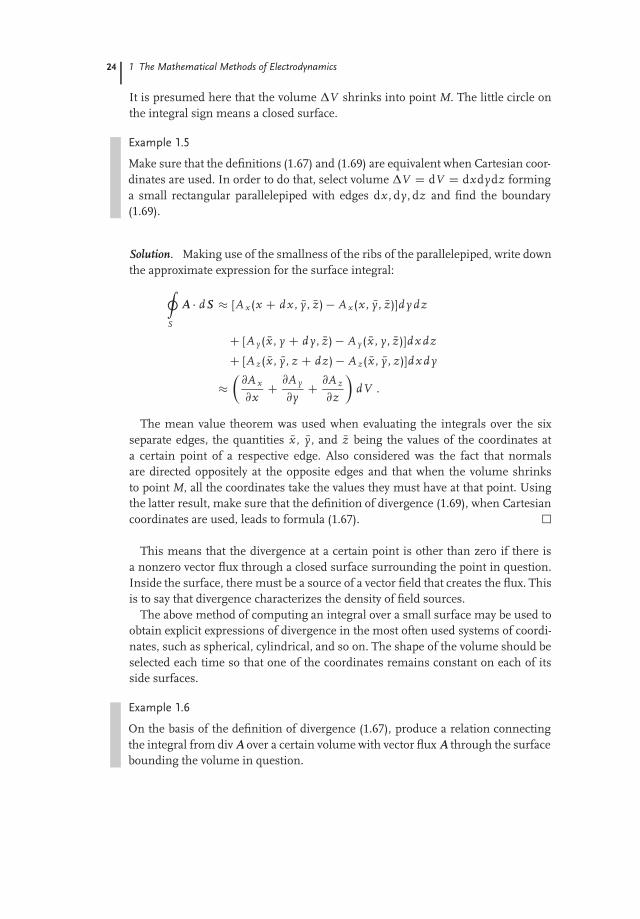
It is presumed here that the volume ΔV shrinks into point M. The little circle onthe integral sign means a closed surface.
Example 1.5
Make sure that the definitions (1.67) and (1.69) are equivalent when Cartesian coor-dinates are used. In order to do that, select volume ΔV D dV D dxdydz forminga small rectangular parallelepiped with edges dx , dy , dz and find the boundary(1.69).
Solution. Making use of the smallness of the ribs of the parallelepiped, write downthe approximate expression for the surface integral:I
S
A � dS � [A x (x C dx , Ny , Nz) � A x (x , Ny , Nz)]d y dz
C [A y ( Nx , y C d y , Nz) � A y ( Nx , y , Nz)]dx dz
C [A z( Nx , Ny , z C dz) � A z( Nx , Ny , z)]dx d y
��
@A x
@xC @A y
@yC @A z
@z
�dV .
The mean value theorem was used when evaluating the integrals over the sixseparate edges, the quantities Nx , Ny , and Nz being the values of the coordinates ata certain point of a respective edge. Also considered was the fact that normalsare directed oppositely at the opposite edges and that when the volume shrinksto point M, all the coordinates take the values they must have at that point. Usingthe latter result, make sure that the definition of divergence (1.69), when Cartesiancoordinates are used, leads to formula (1.67).
This means that the divergence at a certain point is other than zero if there isa nonzero vector flux through a closed surface surrounding the point in question.Inside the surface, there must be a source of a vector field that creates the flux. Thisis to say that divergence characterizes the density of field sources.
The above method of computing an integral over a small surface may be used toobtain explicit expressions of divergence in the most often used systems of coordi-nates, such as spherical, cylindrical, and so on. The shape of the volume should beselected each time so that one of the coordinates remains constant on each of itsside surfaces.
Example 1.6
On the basis of the definition of divergence (1.67), produce a relation connectingthe integral from div A over a certain volume with vector flux A through the surfacebounding the volume in question.

�
� Igor N. Toptygin: Foundations of Classical and Quantum Electrodynamics —Chap. c01 — 2013/10/8 — page 25 — le-tex
�
�
�
�
�
�
1.2 Vector and Tensor Calculus 25
Solution. Select any finite volume V bounded by a smooth closed surface S. Divideit into small cells ΔVi , each bounded by a respective surface ΔSi . The surfacesbounding the cells adjacent to the outside surface S will partially coincide with S.All other portions of the surfaces Si will be shared by pairs of adjacent cells. Makinguse of the smallness of each cell, use relation (1.69), giving it an approximate form:
(div A)i ΔVi �ISi
A � dS i . (1.70)
Now sum the first and second members of the latter approximate equality over iand pass to a limit, reducing the volume of each cell to zero and expanding thenumber of cells to infinity. The first member of the equality will now become anintegral over the full volume V of divergence A:
RV div AdV . In the second member
of the equality, the integrals over the inner portions of the surface will cancel eachother, the outer normals to each pair of adjacent cells being oppositely directed.Only the integral over the outside surface S bounding the full volume V remains.As a result, you will have an exact integral relation,Z
V
div AdV DIS
A � dS , (1.71)
called the Gauss–Ostrogradskii theorem13) (in Western literature, the name Ostro-gradskii is omitted).
The Gauss–Ostrogradskii theorem is applicable to any tensor of rank s � 1, forinstance,Z
V
@Tα�μ
@xμdV D
IS
Tα�μdSμ (1.72)
(for the proof, refer to Problem 1.70�).
The curl of a vector field allows a definition similar to that of divergence (1.69).At point M, specify a unit vector n, that is, a direction. Make up a small flat area ΔScontaining a point M and perpendicular to n. Then define the direction of tracingthe loop l that bounds the area, coordinated with the direction n as per the right-screw rule. The projection of the rotor onto direction n at point M is defined asfollows:
curln A D limΔS!0
1ΔS
Il
A � dl , (1.73)
where the integral represents the circulation of the vector A along the closed loop l.
13) Carl Friedrich Gauss (1777–1855) was an outstanding German mathematician, astronomer, andphysicist. Mikhail Ostrogradskii (1801–1862) was a Russian mathematician known for his worksin mathematical physics, theoretical mechanics, and probability theory.
�
� Igor N. Toptygin: Foundations of Classical and Quantum Electrodynamics —Chap. c01 — 2013/10/8 — page 26 — le-tex
�
�
�
�
�
�
26 1 The Mathematical Methods of Electrodynamics
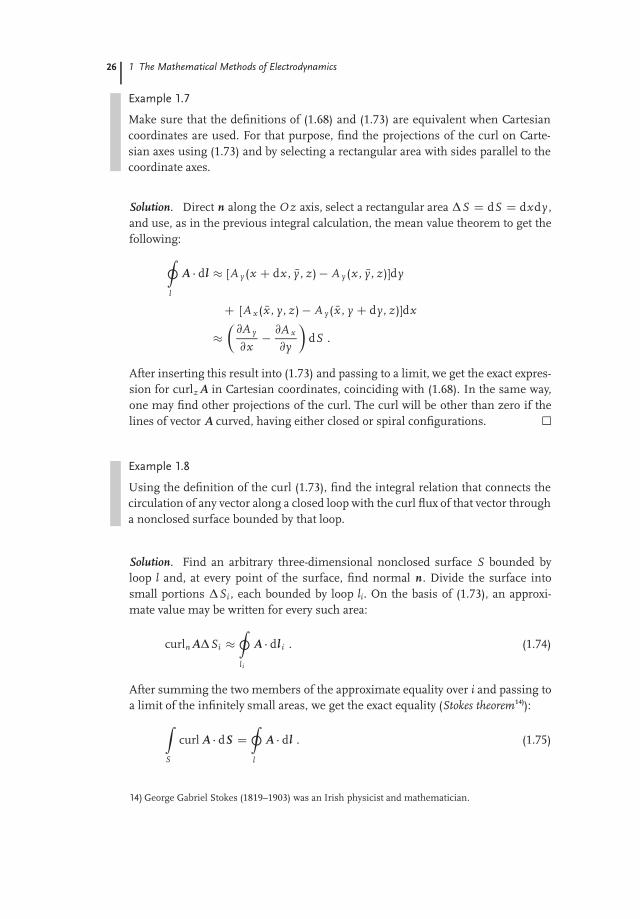
Example 1.7
Make sure that the definitions of (1.68) and (1.73) are equivalent when Cartesiancoordinates are used. For that purpose, find the projections of the curl on Carte-sian axes using (1.73) and by selecting a rectangular area with sides parallel to thecoordinate axes.
Solution. Direct n along the O z axis, select a rectangular area ΔS D dS D dxdy ,and use, as in the previous integral calculation, the mean value theorem to get thefollowing:I
l
A � dl � [A y (x C dx , Ny , z) � A y (x , Ny , z)]dy
C [A x ( Nx , y , z) � A y ( Nx , y C dy , z)]dx
��
@A y
@x� @A x
@y
�dS .
After inserting this result into (1.73) and passing to a limit, we get the exact expres-sion for curlz A in Cartesian coordinates, coinciding with (1.68). In the same way,one may find other projections of the curl. The curl will be other than zero if thelines of vector A curved, having either closed or spiral configurations.
Example 1.8
Using the definition of the curl (1.73), find the integral relation that connects thecirculation of any vector along a closed loop with the curl flux of that vector througha nonclosed surface bounded by that loop.
Solution. Find an arbitrary three-dimensional nonclosed surface S bounded byloop l and, at every point of the surface, find normal n. Divide the surface intosmall portions ΔSi , each bounded by loop li. On the basis of (1.73), an approxi-mate value may be written for every such area:
curln AΔSi �Il i
A � dl i . (1.74)
After summing the two members of the approximate equality over i and passing toa limit of the infinitely small areas, we get the exact equality (Stokes theorem14)):Z
S
curl A � dS DIl
A � dl . (1.75)
14) George Gabriel Stokes (1819–1903) was an Irish physicist and mathematician.

�
� Igor N. Toptygin: Foundations of Classical and Quantum Electrodynamics —Chap. c01 — 2013/10/8 — page 27 — le-tex
�
�
�
�
�
�
1.2 Vector and Tensor Calculus 27
An integral over the outer loop that bounds area S remains in the second member.All integrals over inner loops are canceled. Stokes theorem connects the integralover the curl flux through the surface with the circulation of the vector along theloop that bounds that surface.
1.2.3Solenoidal and Potential (Curl-less) Vectors
Let us say that vector field H (r), over the whole space, satisfies the condition
div H D 0 (1.76)
(in this case, vector H is called a solenoidal vector). This, for instance, is a propertyof a magnetic field. It is possible to prove (we will, for now, abstain from doing that)that condition (1.76) is necessary and sufficient for vector H to be represented asthe curl of another vector A(r):
H D curl A . (1.77)
Using the rules of vector differentiation, we can easily make sure that condition(1.76) is satisfied whatever the value of A is:
div H D r � H D r � [r � A] D [r � r] � A D 0 .
As noted previously, a potential vector is a vector that may be represented as thegradient of a certain scalar function:
E (r) D �grad U(r) � �rU(r) . (1.78)
The necessary and sufficient conditions of the potentiality of a vector are expressedby equalities of the kind in (1.58), which, in their vector form, give the following:
curl E D 0 . (1.79)
Using the definition of the potential vector (1.78) and expressing the curl operationthrough the r operator, we make sure that equality (1.79) is equally valid for anyU(r) functions that have second derivatives.
1.2.4Differential Operations of Second Order
Differential operations of second order appear when the r operator is applied toexpressions of the kind rU , r � A, and r � A that already contain this operator.Using the rules of vector algebra, we find that, in Cartesian coordinates, the Laplace
�
� Igor N. Toptygin: Foundations of Classical and Quantum Electrodynamics —Chap. c01 — 2013/10/8 — page 28 — le-tex
�
�
�
�
�
�
28 1 The Mathematical Methods of Electrodynamics
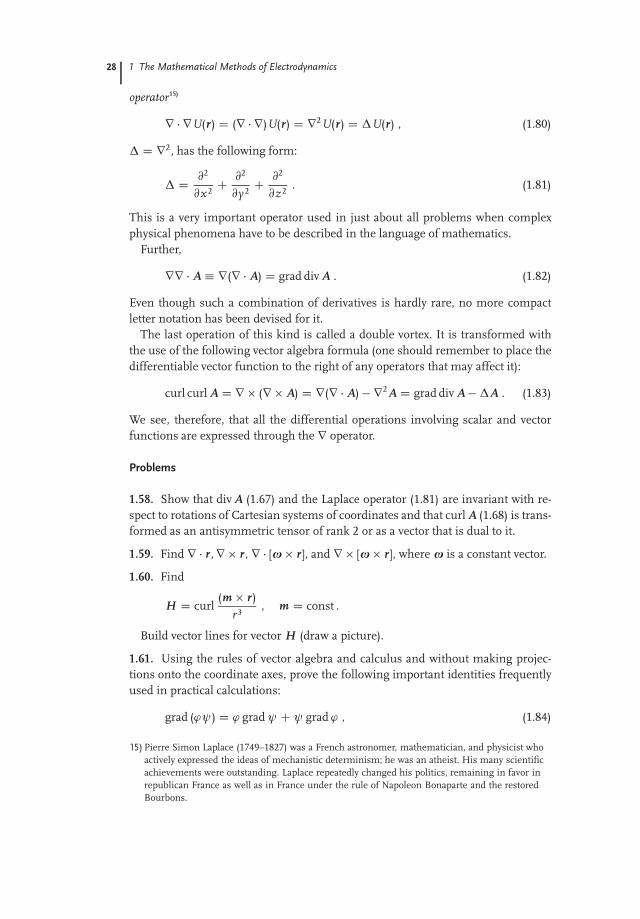
operator15)
r � rU(r) D (r � r)U(r) D r2U(r) D ΔU(r) , (1.80)
Δ D r2, has the following form:
Δ D @2
@x2 C @2
@y 2 C @2
@z2 . (1.81)
This is a very important operator used in just about all problems when complexphysical phenomena have to be described in the language of mathematics.
Further,
rr � A � r(r � A) D grad div A . (1.82)
Even though such a combination of derivatives is hardly rare, no more compactletter notation has been devised for it.
The last operation of this kind is called a double vortex. It is transformed withthe use of the following vector algebra formula (one should remember to place thedifferentiable vector function to the right of any operators that may affect it):
curl curl A D r � (r � A) D r(r � A) � r2A D grad div A � ΔA . (1.83)
We see, therefore, that all the differential operations involving scalar and vectorfunctions are expressed through the r operator.
Problems
1.58. Show that div A (1.67) and the Laplace operator (1.81) are invariant with re-spect to rotations of Cartesian systems of coordinates and that curl A (1.68) is trans-formed as an antisymmetric tensor of rank 2 or as a vector that is dual to it.
1.59. Find r � r , r � r , r � [ω � r ], and r � [ω � r], where ω is a constant vector.
1.60. Find
H D curl(m � r)
r3, m D const .
Build vector lines for vector H (draw a picture).
1.61. Using the rules of vector algebra and calculus and without making projec-tions onto the coordinate axes, prove the following important identities frequentlyused in practical calculations:
grad ('ψ) D ' grad ψ C ψ grad ' , (1.84)
15) Pierre Simon Laplace (1749–1827) was a French astronomer, mathematician, and physicist whoactively expressed the ideas of mechanistic determinism; he was an atheist. His many scientificachievements were outstanding. Laplace repeatedly changed his politics, remaining in favor inrepublican France as well as in France under the rule of Napoleon Bonaparte and the restoredBourbons.

�
� Igor N. Toptygin: Foundations of Classical and Quantum Electrodynamics —Chap. c01 — 2013/10/8 — page 29 — le-tex
�
�
�
�
�
�
1.2 Vector and Tensor Calculus 29
div (' A) D ' div A C A � grad ' , (1.85)
curl ('A) D ' curl A � A � grad ' , (1.86)
div (A � B) D B � curl A � A � curl B , (1.87)
curl (A � B) D A div B � B div A C (B � r)A � (A � r)B , (1.88)
grad (A � B) D A � curl B C B � curl A C (B � r)A C (A � r)B . (1.89)
Here, ' and ψ are the scalar and A, B vector functions of the coordinates.
1.62. Prove the following identities:
C � grad (A � B) D A � (C � r)B C B � (C � r)A , (1.90)
(C � r)(A � B) D A � (C � r)B � B � (C � A , (1.91)
(r � A)B D (A � r)B C B div A , (1.92)
(A � B) � curl C D B � (A � r)C � A � (B � r)C , (1.93)
(A � r) � B D (A � r)B C A � curl B � A div B , (1.94)
(r � A) � B D �A div B C (A � r)B C A � curl B C B � curl A . (1.95)
1.63. Find grad '(r), div '(r)r, curl '(r)r, and (l � r)'(r)r.
1.64. Find a function '(r) that satisfies the condition div '(r)r D 0.
1.65. Find the divergences and curls of the following vectors:
(a � r)b, (a � r)r , '(r)(a � r) , r � (a � r) ,
where a and b are constant vectors.
1.66. Find grad r � A(r), grad A(r) � B(r), div '(r)A(r), curl '(r)A(r), and (l �r)'(r)A(r).
1.67. Prove that
(A � r)A D �A � curl A if A2 D const .
1.68. Transform the integral over volumeR
V (grad ' � curl A)dV into the integralover the surface.
1.69. Express the integrals over the closed surfaceH
S r(a � dS) andH
S (a � r)dS interms of the volume bounded by that surface. Here a is a constant vector.
Hint: Multiply each integral by the arbitrary constant vector b and use the Gauss–Ostrogradskii theorem
�
� Igor N. Toptygin: Foundations of Classical and Quantum Electrodynamics —Chap. c01 — 2013/10/8 — page 30 — le-tex
�
�
�
�
�
�
30 1 The Mathematical Methods of Electrodynamics
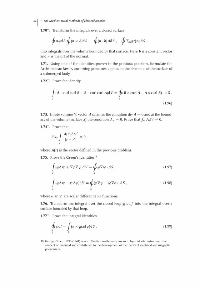
1.70�. Transform the integrals over a closed surfaceIn'dS,
I(n � A)dS ,
I(n � b)AdS ,
ITα�(r)n�dS
into integrals over the volume bounded by that surface. Here b is a constant vectorand n is the ort of the normal.
1.71. Using one of the identities proven in the previous problem, formulate theArchimedean law by summing pressures applied to the elements of the surface ofa submerged body.
1.72�. Prove the identityZV
(A � curl curl B � B � curl curl A)dV DIS
(B � curl A � A � curl B) � dS .
(1.96)
1.73. Inside volume V, vector A satisfies the condition div A D 0 and at the bound-ary of the volume (surface S) the condition A n D 0. Prove that
RV AdV D 0.
1.74�. Prove that
divr
ZV
A(r0)dV 0
jr � r 0j D 0 ,
where A(r) is the vector defined in the previous problem.
1.75. Prove the Green’s identities16)ZV
('Δψ C r'rψ)dV DIS
'rψ � dS , (1.97)
ZV
('Δψ � ψΔ')dV DIS
('rψ � ψr') � dS , (1.98)
where ' an ψ are scalar differentiable functions.
1.76. Transform the integral over the closed loopH
l ud f into the integral over asurface bounded by that loop.
1.77�. Prove the integral identitiesIl
'dl DZS
(n � grad ')dS , (1.99)
16) George Green (1793–1841) was an English mathematician and physicist who introduced theconcept of potential and contributed to the development of the theory of electrical and magneticphenomena.

�
� Igor N. Toptygin: Foundations of Classical and Quantum Electrodynamics —Chap. c01 — 2013/10/8 — page 31 — le-tex
�
�
�
�
�
�
1.2 Vector and Tensor Calculus 31Il
(dl � A) DZS
((n � r) � A)dS , (1.100)
Il
dl � A DZS
(n � r) � AdS . (1.101)
Here n is the ort of the normal to the surface, ' and A are functions of the coordi-nates, l is a closed loop, and S is a nonclosed surface bounded by that loop. Theseidentities may be regarded as special cases of the generalized Stokes theoremI
l
(. . . )dl DZS
(n � r)(. . . )dS , (1.102)
where the symbol (. . . ) labels a tensor of any rank.
1.78. Show that if the scalar function ψ is a solution of the Helmholtz equation17)
4ψ C k2ψ D 0 and a is a certain constant vector, then the vector functions L Drψ, M D r � (aψ), and N D r � M satisfy the Helmholtz vector equation4A C k2A D 0.
1.2.5Differentiating in Curvilinear Coordinates
Unlike in Cartesian rectangular coordinates, when we use curvilinear nonorthog-onal coordinates qα(α D 1, 2, 3), x � (� D 1, 2, 3), the derivative over coordinatesfrom a tensor of rank s � 1 does not produce any tensor, which we will see lat-er. This is due to the local nature of the definition of the tensor (1.51) applicableto a certain point. In the meantime, a derivative is defined through the differenceof the values of two vectors at close but still different points. In order to define acovariant derivative from a tensor of any rank, that is, such a differential operationthat increases the rank of a tensor by one, we will, for simplicity, consider a ten-sor of rank 1 (vector) and expand it in basic vectors of the curvilinear system ofcoordinates in question:
A D Aμ eμ D A μ eμ . (1.103)
Differentiate the equalities in (1.103) and form the covariant derivatives:
A μIα � eμ � @A@qα D @A μ
@qα C A ν eμ � @eν
@qα , (1.104)
AμIα � eμ � @A
@qα D @Aμ
@qα C Aν eμ � @eν
@qα . (1.105)
17) Herman Ludwig Ferdinand Helmholtz (1821–1894) was a German physicist, mathematician,physiologist, and psychologist.

�
� Igor N. Toptygin: Foundations of Classical and Quantum Electrodynamics —Chap. c01 — 2013/10/8 — page 32 — le-tex
�
�
�
�
�
�
32 1 The Mathematical Methods of Electrodynamics
The first members of the equalities use the notation commonly accepted for co-variant derivatives of covariant and contravariant vector components, respectively.The sign of the identity is followed by their definitions. The second members in-clude derivatives of the components of the vector and basic vectors. In curvilinearsystems of coordinates, unlike in Cartesian coordinates, derivatives of basic vectorsare not equal to zero.
Differentiating equality (1.48) over the coordinate, we find that
eμ � @eν
@qα D �eν � @eμ
@qα . (1.106)
Now, add the Christoffel symbols of the second kind to our consideration:18)
Γ νμα D eν � @eμ
@qα . (1.107)
They allow us to write covariant derivatives in a more compact form:
A μIα D @A μ
@qα � A ν Γ νμα , Aμ
Iα D @Aμ
@qα � Aν Γ μνα . (1.108)
Christoffel symbols are not tensors since they do not satisfy the applicable rules oftransformation. They are symmetric as to the two lower symbols: Γ ν
μα D Γ ναμ . The
latter property follows from the representation of basic vectors (1.46):
@eμ
@qαD @eα
@qμ. (1.109)
The rules (1.108) of computing a covariant derivative of a tensor of rank 1 aregeneralized, in an obvious way, to include tensor T of any rank. Besides the deriva-tive over the coordinate from the tensor in question, one needs to add as manyterms with a plus sign as the tensor has upper symbols and as many terms with aminus sign as the tensor has lower symbols.
Example 1.9
Express the Christoffel symbols (1.107) through the components of metric tensorgμν .
Solution. The definition (1.107) of Christoffel symbols allows us to write the fol-lowing relation:
eν Γ νμα D @eμ
@qα . (1.110)
It follows from the equality (eν )λ(eν )σ D δσλ , which follows from the representa-
tions of basic vectors (1.46) and (1.49).
18) Elwin Bruno Christoffel (1829–1900) was a German mathematician.

�
� Igor N. Toptygin: Foundations of Classical and Quantum Electrodynamics —Chap. c01 — 2013/10/8 — page 33 — le-tex
�
�
�
�
�
�
1.2 Vector and Tensor Calculus 33
If we use the relation,
eν Γν,μα D @eμ
@qα , (1.111)
Also consider Christoffel symbols of the first kind, Γν,μα
As follows from (1.110) and (1.111), Christoffel symbols of the first and secondkinds may be regarded as the coefficients of the expansion of the quantity @eμ/@qα
in vectors of covariant and contravariant bases.Using (1.48), we find from (1.111) that
Γν,μα D eν � @eμ
@qα . (1.112)
Multiplying (1.110), in a scalar way, by eλ and (1.111) by eλ and using (1.50), wefind the connection between Christoffel symbols of the first and second kinds:
Γν,μα D gνλ Γ νμα , Γ ν
μα D gνλ Γν,μα . (1.113)
Then, sequentially using the symmetry of the two symbols separated by a commaand relations (1.109), (1.112), and (1.113), find the following:
Γν,μα D 12
�eν � @eμ
@qα C eν � @eα
@qμ
�
D 12
�@gμν
@qαC @gαν
@qμ� eμ � @eν
@qα� eα � @eν
@qμ
�
D 12
�@gμν
@qα C @gαν
@qμ � @gαμ
@qν
�, (1.114)
Γ νμα D 1
2gνλ
�@gμλ
@qα C @gαλ
@qμ � @gαμ
@qν
�. (1.115)
Example 1.10
Find the rules of the transformation of Christoffel symbols of the first and secondkinds when they are transferred to another curvilinear coordinate system.
Solution. Do the sequential computations
Γ 0νμα D e0ν � @e0
μ
@q0αD @q0ν
@q�e� � @
@q0α
@qσ
@q0μeσ
D @q0ν
@q�
@qλ
@q0α
@qσ
@q0μe� � @eσ
@qλC @q0ν
@q�
@qλ
@q0α
@q0�
@qλ
@2qσ
@q0�@q0μe� � eσ

�
� Igor N. Toptygin: Foundations of Classical and Quantum Electrodynamics —Chap. c01 — 2013/10/8 — page 34 — le-tex
�
�
�
�
�
�
34 1 The Mathematical Methods of Electrodynamics
D @q0ν
@q�
@qλ
@q0α
@qσ
@q0μ Γ �λσ C @q0ν
@q�
@2q�
@q0α@q0μ , (1.116)
Γ 0ν,μα D e0
ν � @e0μ
@q0α D @q�
@q0ν e� � @
@q0α
@qσ
@q0μ eσ
D @q�
@q0ν
@qλ
@q0α
@qσ
@q0μ e� � @eσ
@qλ C @q�
@q0ν
@2qσ
@q0α@q0μ e� � eσ
D @q�
@q0ν
@qλ
@q0α
@qσ
@q0μ Γ�,λσ C @q�
@q0ν
@2q�
@q0α@q0μ g�σ . (1.117)
Only the first terms in the second members of the resulting expressions conformto the rules of the transformation of tensors. The second terms violate the saidrules, which means that Christoffel symbols are not tensors.
Example 1.11
Prove that the covariant derivatives of the vectors A νIα and AνIα are transformed ascovariant and mixed tensors, respectively, of rank 2.
Solution. Using the definition of covariant derivative (1.104) and the rule of trans-formation (1.116), sequentially find the following:
A0μIα D @A0
μ
@q0α� Γ 0ν
μα A0ν
D @
@qλ
�@qσ
@q0μ A σ
�@qλ
@q0α
�
@q0ν
@q�
@qλ
@q0α
@qσ
@q0μΓ �
λσ C @q0ν
@q�
@2q�
@q0α@q0μ
!@q�
@q0νA �
D @qσ
@q0μ
@qλ
@q0α
�@A σ
@qλ � Γ �λσ A �
�D @qσ
@q0μ
@qλ
@q0α A σIλ . (1.118)
It has been proven that the quantity in question is transformed as a covariant ten-sor of rank 2. When considering the second tensor, one must use the followingequality:
@q0ν
@q�
@2q�
@q0α@q0μ D @q�
@q0α
@qλ
@q0μ
@2q0ν
@q�@qλ . (1.119)
It follows from differentiating over the coordinate of an equality such as (1.43).

�
� Igor N. Toptygin: Foundations of Classical and Quantum Electrodynamics —Chap. c01 — 2013/10/8 — page 35 — le-tex
�
�
�
�
�
�
1.2 Vector and Tensor Calculus 35
Problems
1.79. Show that a derivative of a coordinate of the scalar (gradient) @S/@qμ D SIμ
is a covariant vector.
1.80. Show that a covariant curl coincides with a proper curl:
A μIν � A νIμ D @A μ
@qν � @A ν
@qμ .
1.81�. Show that the covariant divergence of a covariant vector (scalar) may bewritten as
AμIμ D 1p
g@
@qμ
�pgAμ� . (1.120)
1.82. In curvilinear coordinates, write down the Laplace operator influencing ascalar function.
1.83. Write down covariant divergence T μνIμ for any tensor of rank 2.
1.84. Do the same for the antisymmetric tensor Aμν D �Aνμ.
1.85. Prove the following relation for the covariant components of the antisymmet-ric tensor A μν D �A νμ:
A μνIλ C A λμIν C A νλIμ D @A μν
@qλ C @A λμ
@qν C @A νλ
@qμ .
1.86. Find the covariant derivatives of the metric tensor gμνIλ and gνμIλ .
1.87. Prove the identity @gμν/@qλ D Γμ,νλ C Γν,μλ.
1.2.6Orthogonal Curvilinear Coordinates
Orthogonal curvilinear coordinates in which gμν D 0 while μ ¤ ν (see Prob-lem 1.46) are practically used very frequently. In those cases, the following notationis used: gμν D h2
μ(q)δμν (no summing over μ is necessary). The element of lengthis written as
dl2 D gμνdqμdqν D h21(dq1)2 C h2
2(dq2)2 C h23(dq3)2 , (1.121)
where, in accordance with (1.46), values hμ (Lamé coefficients)19) have the followingform:
hμ Ds�
@x@qμ
�2
C�
@y@qμ
�2
C�
@z@qμ
�2
. (1.122)
19) Gabriel Lamé (1795–1870) was a French mathematician and engineer who conducted research inmathematical physics and the theory of elasticity.

�
� Igor N. Toptygin: Foundations of Classical and Quantum Electrodynamics —Chap. c01 — 2013/10/8 — page 36 — le-tex
�
�
�
�
�
�
36 1 The Mathematical Methods of Electrodynamics
Sincep
g D h1h2h3, the invariant volume element (1.54) assumes the followingform:
dV D h1h2h3dq1dq2dq3 . (1.123)
The characteristic peculiarity of an orthogonal basis is that the vectors of the orig-inal and mutual bases have the same directions but different sizes and physicaldimensions (because the coordinates x α and q� may have different dimensions).This is why the dimensions of different components of the same vector, expandedin the vectors of those bases, may also be different, which creates a certain incon-venience when physical problems are being solved. This is why the introductionof an orthogonal basis of unit vectors eα�, eα� � e�� D δα� is useful (we will labelthem with lower indices and an asterisk) and through which, in accordance with(1.50), the covariant and contravariant bases will be expressed in the following way:
e� D h� e�� , e� D 1h�
e�� . (1.124)
The expansion of an arbitrary vector A in orts e�� assumes the following form:
A D A 1�e1� C A 2�e2� C A 3�e3� , (1.125)
where the “physical” components of the vector A μ� now have the same dimension-ality matching that of A, that is, the physical quantity in question, and are connect-ed to its covariant and contravariant components by the following relations:
A �� D A μ
hμD Aμ hμ . (1.126)
Since the use of the basis e�� is convenient, hereafter we will use that basis every-where, omitting the asterisk.
Using relations (1.120)–(1.126), and also (1.25), write down the principal opera-tions of differentiation in orthogonal curvilinear coordinates:
grad S D 1h1
@S@q1
e1 C 1h2
@S@q2
e2 C 1h3
@S@q3
e3 I (1.127)
div A D 1h1h2h3
�@
@q1 (h2h3A 1) C @
@q2 (h1h3A 2) C @
@q3 (h1h2A 3)�
I(1.128)
ΔS D 1h1h2h3
�@
@q1
�h2h3
h1
@S@q1
�C @
@q2
�h1h3
h2
@S@q2
�C @
@q3
�h1h2
h3
@S@q3
��I (1.129)

�
� Igor N. Toptygin: Foundations of Classical and Quantum Electrodynamics —Chap. c01 — 2013/10/8 — page 37 — le-tex
�
�
�
�
�
�
1.2 Vector and Tensor Calculus 37
curlA D 1h2h3
�@
@q2(h3A 3) � @
@q3(h2A 2)
�e1
C 1h1h3
�@
@q3(h1A 1) � @
@q1(h3A 3)
�e2
C 1h1h2
�@
@q1 (h2A 2) � @
@q2 (h1A 1)�
e3 . (1.130)
Problems
1.88. From the common expressions (1.27)–(1.29), derive the basic differential op-erations below in the (r, α, z) cylindrical coordinate system where x D r cos α,y D r sin α, and z D z:
grad S D @S@r
e r C 1r
@S@α
eα C @S@z
ez I (1.131)
div A D 1r
@
@r(r A r) C 1
r@A α
@αC @A z
@zI (1.132)
ΔS D 1r
@
@r
�r@S@r
�C 1
r2
@2S@α2 C @2 S
@z2 I (1.133)
curl A D�
1r
@A z
@α� @A α
@z
�e r C
�@A r
@z� @A z
@r
�eα
C 1r
�@
@r(r A α) � @A r
@α
�ez . (1.134)
1.89. Do the same for the (r, #, α) spherical coordinate system where x Dr sin # cos α, y D r sin # sin α, and z D r cos # :
grad S D @S@r
e r C 1r
@S@#
e# C 1r sin #
@S@α
eα I (1.135)
div A D 1r2
@
@r(r2A r) C 1
r sin #
@
@#(A# sin #) C 1
r sin #
@A α
@αI (1.136)
ΔS D 1r2
@
@r
�r2 @S
@r
�C 1
r2 sin #
@
@#
�sin #
@S@#
�C 1
r2 sin2 #
@2S@α2 I (1.137)
curl A D 1r sin #
�@
@#(A α sin #) � @A#
@α
�e r
C�
1r sin #
@A r
@α� 1
r@
@r(r A α)
�e# C 1
r
�@
@r(r A# ) � @A r
@#
�eα .
(1.138)
�
� Igor N. Toptygin: Foundations of Classical and Quantum Electrodynamics —Chap. c01 — 2013/10/8 — page 38 — le-tex
�
�
�
�
�
�
38 1 The Mathematical Methods of Electrodynamics
1.90�. Use identity (1.83) to write the projections of the vector 4A onto the axesof a cylindrical coordinate system.
1.91�. Do the same for a spherical coordinate system.
1.92. Find the general form solution of Laplace’s equation for a scalar function thatdepends only on (i) r, (ii) α, and (iii) z (cylindrical coordinates).
1.93. Find the general form solution of Laplace’s equation for a scalar function thatdepends only on (i) r, (ii) # , and (iii) α (spherical coordinates).
Note In Problems 1.94�–1.98�, examples of curvilinear orthogonal systems ofcoordinates are considered. These systems are more complex than cylindrical andspherical systems. For more information, see Arfken (1970) and Stratton (1948)
1.94�. The equation
x2
a2 C y 2
b2 C z2
c2 D 1 (a > b > c)
represents an ellipsoid with semiaxes a, b, and c. The equations
x2
a2 C �C y 2
b2 C �C z2
c2 C �D 1 , � � �c2 ,
x2
a2 C ηC y 2
b2 C ηC z2
c2 C ηD 1 , �c2 � η � �b2 ,
x2
a2 C �C y 2
b2 C �C z2
c2 C �D 1 , �b2 � � � �a2
represent an ellipsoid and one-sheet and two-sheet hyperboloids confocal with thefirst ellipsoid, respectively. Each point of the space is crossed by a surface character-ized by values � , η, and � . � , η, and � are called ellipsoidal coordinates of the pointx , y , z. Find the formulas of transformation of ellipsoidal to Cartesian coordinates.Make sure that an ellipsoidal system of coordinates is orthogonal. Find the Lamécoefficients and Laplace’s operator in ellipsoidal coordinates.
1.95�. When a D b > c, the ellipsoidal coordinate system (see the previous prob-lem) degenerates to become a so-called flattened spheroidal coordinate system.When this happens, the coordinate � becomes constant, equals �a2, and mustbe replaced by another coordinate. To serve as such, an azimuthal angle α on thesurface x y is selected. The coordinates � and η are found from the following equa-tions:
r2
a2 C �C z2
c2 C �D 1 , � � �c2 ,
r2
a2 C ηC z2
c2 C ηD 1 , �c2 � η � �a2 ,

�
� Igor N. Toptygin: Foundations of Classical and Quantum Electrodynamics —Chap. c01 — 2013/10/8 — page 39 — le-tex
�
�
�
�
�
�
1.2 Vector and Tensor Calculus 39
where r2 D x2 C y 2.Surfaces � D const are flattened ellipsoids of rotation around the O z axis. Sur-
faces η D const are one-sheet hyperboloids of rotation confocal with them (Fig-ure 1.6).
Figure 1.6 A flattened spheroidal system of coordinates.
Find the expressions for r and z in flattened spheroidal coordinates, the Lamécoefficients, and Laplace’s operator in those coordinates.
1.96�. An extended spheroidal system of coordinates is derived from an ellipsoidalone (Problem 1.94�) when a > b D c. When this happens, the coordinate ηbecomes constant and must be replaced with an azimuthal angle α marked offon the y z surface by the O y axis. The coordinates � and � are found from thefollowing equations:
x2
a2 C �C r2
b2 C �D 1 , � � �b2 ,
x2
a2 C �C r2
b2 C �D 1 , �b2 � � � �a2 ,
where r2 D y 2 C z2.The surfaces of the constants � and η are extended ellipsoids and two-sheet
hyperboloids of rotation (Figure 1.7). Express the quantities x and r through � and� . Find the Lamé coefficients and Laplace’s operator in the variables � , � , and α.
1.97�. Bispherical cooordinates � , η, and α are connected to Cartesian coordinatesby the following relations:
x D a sin η cos αcosh � � cos η
, y D a sin η sin αcosh � � cos η
, z D a sinh �cosh � � cos η
,
where a is a constant parameter, �1 < � < 1, 0 < η < π, and 0 < α < 2π.Show that the coordinate surfaces � D const are spheres,
x2 C y 2 C (z � a coth � )2 D�
asinh �
�2
,

�
� Igor N. Toptygin: Foundations of Classical and Quantum Electrodynamics —Chap. c01 — 2013/10/8 — page 40 — le-tex
�
�
�
�
�
�
40 1 The Mathematical Methods of Electrodynamics
Figure 1.7 An extended spheroidal system of coordinates.
the surfaces η D const are spindle-shaped surfaces of rotation around the O z axis,whose equation is�q
x2 C y 2 � a cot η�2
C z2 D�
asin η
�2
,
and surfaces α D const are half-planes diverging from the O z axis (Figure 1.8).Make sure that these coordinate surfaces are orthogonal with respect to each other.Find the Lamé coefficients and Laplace’s operator.
Figure 1.8 A bispherical system of coordinates.
1.98�. The toroidal coordinates �, � , and α make up an orthogonal system and areconnected to Cartesian coordinates by the following relations:
x D a sinh � cos αcosh � � cos �
, y D a sinh � sin αcosh � � cos �
, z D a sin �cosh � � cos �
,

�
� Igor N. Toptygin: Foundations of Classical and Quantum Electrodynamics —Chap. c01 — 2013/10/8 — page 41 — le-tex
�
�
�
�
�
�
1.3 The Special Functions of Mathematical Physics 41
where a is a constant parameter, �1 < � < 1, �π < � < π, and 0 < α < π.Show that � D ln(r1/r2) (see Figure 1.9, displaying the surfaces α D const and
α C π D const) and the quantity � is the angle between r1 and r2 (� > 0 if z > 0and � < 0 if z < 0). What is the form of the coordinate surfaces � D const and� D const? Find the Lamé coefficients.
Figure 1.9 A toroidal system of coordinates.
Suggested literature:Borisenko and Tarapov (1966); Weinberg (1972); Arfken (1970); Mathews and Walk-er (1964); Lee (1965); Rashevskii (1953); Morse and Feshbach (1953); Stratton(1948); Madelung (1957)
1.3The Special Functions of Mathematical Physics
1.3.1Cylindrical Functions
Cylindrical functions are used when solving many specific problems. Of these, theBessel functions are the most commonly used. They may be obtained by expandinga purposely selected exponent (generating function) in a power series over u:
exp�
x2
�u � 1
u
�D
1XnD�1
Jn(x )un . (1.139)
The coefficients Jn(x ) of this expansion are called Bessel functions20) of the firstkind and order n. The representation of a Bessel function as a power series may be
20) Friedrich Wilhelm Bessel (1784–1846) was a German astronomer, land surveyor, andmathematician.

�
� Igor N. Toptygin: Foundations of Classical and Quantum Electrodynamics —Chap. c01 — 2013/10/8 — page 42 — le-tex
�
�
�
�
�
�
42 1 The Mathematical Methods of Electrodynamics
obtained from the power series for exponents:
exp x u
2
�exp
� x
2u
�D
1XrD0
x2
�r ur
r!
1XsD0
(�1)s x
2
�s u�s
s!. (1.140)
These expansions are valid for any (including complex) values of x and u, which isdue to the unboundedness of the radius of convergence of an exponent. Changingto summing over n D r � s(�1 < n < 1), we get, from (1.140)
exp�
x2
�u � 1
u
�D
1XnD�1
1XsD0
(�1)s
s!(n C s)!
x2
�nC2sun
D1X
nD�1Jn(x )un , (1.141)
wherefrom it follows that
Jn(x ) D1X
sD0
(�1)s
s!(n C s)!
x2
�nC2s. (1.142)
The use of this representation for Jn(x ) is expedient when n � 0. When n < 0, thefollowing may be written instead of (1.142):
Jn(x ) D1X
sDjnj
(�1)s
s!(n C s)!
x2
�nC2s D1X
sD0
(�1)sCjnj
s!(jnj C s)!
x2
�jnjC2sun . (1.143)
This is because when s C n < 0, (s C n)! ! 1. As a result, we get a simple depen-dence between the Bessel functions of the whole positive and negative orders:
J�n(x ) D (�1)n Jn(x ) . (1.144)
Example 1.12
Obtain recurrent relations between Bessel functions of various orders by differen-tiating equality (1.139) over u and over x, comparing the second and first membersof the equality.
Solution. Differentiating (1.139) over u, we get
x2
�1 C 1
u2
�exp
�x2
�u � 1
u
��D x
2
�1 C 1
u2
� 1XnD�1
Jn(x )un
D1X
nD�1n Jn(x )un�1 .
�
� Igor N. Toptygin: Foundations of Classical and Quantum Electrodynamics —Chap. c01 — 2013/10/8 — page 43 — le-tex
�
�
�
�
�
�
1.3 The Special Functions of Mathematical Physics 43
Equating the coefficients of un�1 in second and first members of the latter equality,we find the following:
Jn�1(x ) C JnC1(x ) D 2nx
Jn(x ) . (1.145)
Differentiating (1.139) over x, we get in the same way
Jn�1(x ) � JnC1(x ) D 2 J 0n(x ) . (1.146)
These recurrent relations may be rewritten as follows, in other forms:
Jn˙1 D nx
Jn(x ) � J 0(x ) I Jn�1 D ˙x�n ddx
[x˙n Jn(x )] . (1.147)
Specifically,
J1(x ) D � J 00(x ) . (1.148)
Example 1.13
Obtain representations of the Bessel function as integrals from exponential andtrigonometric functions. For that purpose, use the substitution u D exp(i') inexpansion (1.139).
Solution. The substitution leads to the expansion
exp(i x sin ') D1X
nD�1Jn(x ) exp(i n') . (1.149)
Use the periodicity of the functions sin ' and exp(i n') and also the easily verifiableequality
αC2πZα
exp(i(n � m)')d' D 2πδmn ,
where m is an integer and α is any real number. Multiplying both parts of (1.149) byexp(�i m') and integrating over ', we get the representation of the Bessel function:
Jm(x ) D 12π
αC2πZα
exp(i x sin ' � i m')d'
D (�i)m
2π
αC2πZα
exp(i x cos ' � i m')d' . (1.150)

�
� Igor N. Toptygin: Foundations of Classical and Quantum Electrodynamics —Chap. c01 — 2013/10/8 — page 44 — le-tex
�
�
�
�
�
�
44 1 The Mathematical Methods of Electrodynamics
Example 1.14
Presume that certain functions of Zν (x ), different, generally speaking, from Besselfunctions (1.142), satisfy the recurrent relations (1.145)–(1.148) when the value ofn D ν is arbitrary and complex. Produce a differential equation of the second orderwhose solution is Zν (x ).
Solution. Differentiate the second equality (1.147) over x and add a term equalingzero to it (replacing n ! ν, Jn ! Zν ):
Z 0ν�1 D [x�ν (x ν Zν)0]0 C 1
x
Z 0
ν C νx
Zν � Zν�1
�D Z 00
ν C ν C 1x
Z 0ν � 1
xZν�1 .
Once again, add a term equaling zero to the second member:
Z 0ν�1 D Z 00
ν C ν C 1x
Z 0ν � 1
xZν�1 C n
x
hZν�1 � ν
xZν � Z 0
ν
iD Z 00
ν C 1x
Z 0ν � n2
x2 Zν C ν � 1x
Zν�1 .
Finally, from the second equality in (1.147), if we make the replacement n C 1 !ν, Jn ! Zν , we find
Zν D ν � 1x
Zν�1 � Z 0ν�1 .
Excepting Z 0ν�1 from the latter two equalities, we get the Bessel equation, satisfied
by the function Zν(x ):
Z 00ν C 1
xZ 0
ν C�
1 � ν2
x2
�Zν D 0 . (1.151)
This or a similar equation appears when solving many physical problems. Below,we will briefly summarize the basic information concerning the solutions of thisequation. The generation of the necessary formulas is shown in special mathemat-ical texts (Arfken, 1970; Nikiforov and Uvarov, 1988; Gradshtein and Ryzhik, 2007;Lee, 1965; Mathews and Walker, 1964; Abramovitz and Stegun, 1965; Vilenkin,1988).
A solution of (1.151), limited when Reν � 0, called a Bessel function of the firstorder when x ! 0, may be represented as a power series, which is a generalizationof (1.142):
Jν(z) D z
2
�ν 1XsD0
(�1)s
s!Γ (ν C s C 1)
z2
�2s. (1.152)
�
� Igor N. Toptygin: Foundations of Classical and Quantum Electrodynamics —Chap. c01 — 2013/10/8 — page 45 — le-tex
�
�
�
�
�
�
1.3 The Special Functions of Mathematical Physics 45
The independent variable is labeled z, because the series remains valid whateverthe values of ν and throughout the complex plane z, except for the slit along thenegative part of the real axis.
Another linearly independent solution, when ν ¤ n D 0, ˙1, . . ., may be J�ν(x ).When n is an integer, there is a linear connection (1.144) between the two solutionsshown. This is why the Bessel function of the second kind (the same as Neumann’sfunction21) or Weber’s function22)) is selected as the second solution:
Yν(z) D Jν(z) cos νπ � J�ν (z)sin νπ
. (1.153)
This solution has a finite bound when ν ! n.Also, Bessel functions of the third order, also called Hankel functions23), may be
selected as two linearly independent solutions:
H (1)ν (z) D Jν(z) C i Yν(z) I H (2)
ν (z) D Jν(z) � i Yν(z) . (1.154)
All these functions are solutions of Bessel’s equation. The functions Yν and H (1,2)ν
have singularities when z ! 0. All these solutions satisfy the recurrent relations(1.145)–(1.147) (with the replacement of n ! ν, Jn ! Zν).
The asymptotic values are as follows: when z ! 0,
Jν(z) � z ν
2ν Γ (ν C 1), ν ¤ �1, �2, . . . , (1.155)
Y0(z) � �i H (1)0 (z) � i H (2)
0 (z) � 2π
ln z , (1.156)
Yν(z) � �i H (1)ν (z) � i H (2)
ν (z) � � Γ (ν)π
z2
��ν, Reν > 0 , (1.157)
and when jzj ! 1 and ν is arbitrary,
Jν(z) �r
2πz
cos
z � νπ2
� π4
�, j arg zj < π , (1.158)
Yν(z) �r
2πz
sin
z � νπ2
� π4
�, j arg zj < π , (1.159)
H (1)ν (z) �
r2
πzexp
hi
z � νπ2
� π4
�i, �π < arg z < 2π , (1.160)
H (2)ν (z) �
r2
πzexp
h�i
z � νπ2
� π4
�i, �2π < arg z < π . (1.161)
21) Karl Gottfried Neumann (1832–1925) was a German mathematician.22) Heinrich Weber (1842–1913) was a German mathematician.23) Hermann Hankel (1839–1873) was a German mathematician and a historian of mathematics.
�
� Igor N. Toptygin: Foundations of Classical and Quantum Electrodynamics —Chap. c01 — 2013/10/8 — page 46 — le-tex
�
�
�
�
�
�
46 1 The Mathematical Methods of Electrodynamics
Cylindrical functions of purely imaginary arguments are called modified Besselfunctions. The second of them is also called the Macdonald function.24) They aredescribed by the following relations:
Iν(z) D e�i πν/2 Jν (i z) , (1.162)
Kν(z) D π2
e i π(νC1)/2H (1)ν (i z) (1.163)
or
Iν(z) D z
2
�ν 1XsD0
(z/2)2s
s!Γ (ν C s C 1), Kν(z) D π
2I�ν(z) � Iν(z)
sin νπ. (1.164)
These functions take real values when ν and z > 0 are real. Recurrent relation anddifferentiation formulas are produced from (1.145)–(1.147), (1.162), and (1.163).For instance,
I 00(z) D I1(z) , K 0
0(z) D �K1(z) . (1.165)
Modified Bessel functions satisfy the equation
W 00ν C 1
zW 0
ν ��
1 C ν2
z2
�Wν D 0 . (1.166)
The asymptotic values are as follows: when z ! 0,
Iν(z) � z ν
2ν Γ (ν C 1), ν ¤ �1, �2 . . . , (1.167)
K0(z) � � ln z , Kν(z) � 12
Γ (ν) z
2
��ν, Reν > 0 , (1.168)
and when jzj ! 1,
Iν(z) � 1p2πz
ez , j arg zj <π2
, (1.169)
Kν(z) �r
π2z
e�z , j arg zj <3π2
. (1.170)
The spherical functions of Bessel, Hankel, and Weber often appear when prob-lems are solved in spherical coordinates. They are of half-integer order and aredescribed by the following equalities:
j l(x ) Dr
π2x
JlC 12(x ) I h(1,2)
l Dr
π2x
H (1,2)lC 1
2(x ) I
y l(x ) Dr
π2x
YlC 12(x ) . (1.171)
24) Hector Munro Macdonald (1865–1935) was a Scottish physicist and mathematician.

�
� Igor N. Toptygin: Foundations of Classical and Quantum Electrodynamics —Chap. c01 — 2013/10/8 — page 47 — le-tex
�
�
�
�
�
�
1.3 The Special Functions of Mathematical Physics 47
All these functions (their common symbol is zl (x )) satisfy the following equation:
z00l C 2
xz0
l C�
1 � l(l C 1)x2
�zl D 0 .
When x is small,
j l(x ) � x l
1 � 3 � � � (2l C 1), h(1,2)
l � � x�l�1
1 � 3 � � � (2l � 1). (1.172)
When x is large,
j l(x ) � 1x
cos�
x � (l C 1)π2
�,
h(1,2)l (x ) � 1
xexp
�˙�
x � (l C 1)π2
�. (1.173)
Problems
1.99. Compute the indefinite integralsRx ν Zν�1(x )dx and
Rx�ν ZνC1(x )dx .
1.100. Compute the definite integralsR10 J1(x )dx ,
R10 J2(x )x�1dx , and
R10 Jn(x )x�ndx .
1.101. Prove the equality of the integralsR10 Jn(x )dx D R1
0 Jn(x )dx , n D 0, 1, . . .
1.102. Obtain the integral representation
J0(x ) D 2π
1Z0
cos uxp1 � u2
du .
Hint: Perform the substitution u D sin '.
1.103� . Compute the integrals
π/2Z0
J0(x cos ') cos 'd' D sin xx
and
π/2Z0
J1(x cos ')d' D 1 � cos xx
.
Hint: You may use expansion in power series.
1.104. Produce the formulas
Jn(x ) D (�1)k x n�
dxdx
�k x k�n Jn�k(x )
�D (�1)n x n
�d
xdx
�n
J0(x ) .

�
� Igor N. Toptygin: Foundations of Classical and Quantum Electrodynamics —Chap. c01 — 2013/10/8 — page 48 — le-tex
�
�
�
�
�
�
48 1 The Mathematical Methods of Electrodynamics
1.105. Produce recurrent relations for the modified Bessel functions:
Iν�1(z) � IνC1(z) D 2νz
Iν(z) I Iν�1(z) C IνC1(z) D 2I 0ν(z) I (1.174)
Kν�1(z) � KνC1(z) D � 2νz
Kν (z) IKν�1(z) C KνC1(z) D �2K 0
ν (z) . (1.175)
1.106�. Show that
J0(jr1 � r2j) D1X
nD�1Jn(r1) Jn(r2) exp(i n#) ,
where # is the angle between vectors r1 and r2.
1.107�.
1. Write an equation satisfied by the function u(x ) D Jn(ax ).2. Compute the integral (b ¤ a)
1Z0
x Jn(ax ) Jn(bx )dx D a J 0n(a) Jn(b) � b J 0
n(b) Jn(a)b2 � a2
. (1.176)
3. a ¤ b are the roots of the equation Jn(x ) D 0, that is, Jn(a) D Jn(b) D 0. Showthat
1Z0
x Jn(ax ) Jn(bx )dx D 0 and
1Z0
x J2n(ax )dx D 1
2[ J 0
n(a)]2 . (1.177)
Note The first equality (1.177) expresses the property called the orthogonality ofBessel functions weighted by x.
1.108�. Produce “summation theorems” for Bessel functions:
1XkD�1
Jn�k (x ) Jk (y ) D Jn(x C y ) , n D 0, 1, 2, . . . I (1.178)
1XkD�1
(�1)k Jn�k (x ) Jk (x ) D 0 , n D 1, 2, . . . I (1.179)
J0(x ) J0(y ) C 21X
kD1
(�1)k Jk (x ) Jk (y ) D J0(x C y ) , n D 1, 2, . . . I (1.180)
J20 (x ) C 2
1XkD1
(�1)k J2k (x ) D J0(2x ) . (1.181)

�
� Igor N. Toptygin: Foundations of Classical and Quantum Electrodynamics —Chap. c01 — 2013/10/8 — page 49 — le-tex
�
�
�
�
�
�
1.3 The Special Functions of Mathematical Physics 49
1.3.2Spherical Functions and Legendre Polynomials
Spherical functions and Legendre polynomials are widely used in many fields ofphysics, especially in electrodynamics and quantum mechanics. The generatingfunction for Legendre polynomials25) Pl(cos #) is the reverse distance between twopoints with radius vectors a and r , the angle between them equaling # :
1jr � aj D 1p
r2 C a2 � 2ar cos #D 1
r
1XlD0
ar
�lPl (cos #) ,
ar
< 1 .
(1.182)
Designating x D cos # and u D a/r and using binomial expansion, which, for thenegative exponents is conveniently written as
(1 � α)�q D1X
nD0
Γ (n C q)n!Γ (q)
αn , jαj < 1 ,
and the binomial expansion for αn D (2ux � u2)n , we get a double sum:
(1 � 2ux C u2)�1/2 D1X
nD0
nXkD0
Γ (n C 1/2)Γ (1/2)k!(n � k)!
(�1)k (2x )n�k unCk .
Begin summing over k and n C k D l � 0, which will result in the rearrangementof the terms of the series. In this case, this rearrangement is valid because theinfinite series is absolutely convergent, which will be shown below. As the result,we have
(1 � 2ux C u2)�1/2 D1X
lD0
lXkD0
Γ (l � k C 1/2)Γ (1/2)k!(l � 2k)!
(�1)k (2x )l�2k ul
D1X
lD0
Pl (x )ul ,
where
Pl(x ) DlX
kD0
Γ (l � k C 1/2)Γ (1/2)k!(l � 2k)!
(�1)k (2x )l�2k
DlX
kD0
(�1)k (2l � 2k)!2l k!(l � k)!(l � 2k)!
x l�2k . (1.183)
In the latter two equalities, the sum over k is actually limited to the value of theinteger part of l/2 because the infinite factorial of the negative integer in the de-nominator will eliminate all terms with l � 2k < 0.
25) Adrien-Marie Legendre (1752–1833) was a French mathematician.

�
� Igor N. Toptygin: Foundations of Classical and Quantum Electrodynamics —Chap. c01 — 2013/10/8 — page 50 — le-tex
�
�
�
�
�
�
50 1 The Mathematical Methods of Electrodynamics
Example 1.15
Find the values of the polynomials Pl (1), Pl (�1), and Pl (0) by assigning particularvalues to the angle # in (1.182) and using the binomial expansion.
Solution. If we assume that cos # D 1, we find, from (1.182), that
11 � u
D1XlD0
ul D1X
lD0
Pl (1)ul
and, therefore, Pl (1) D 1 whatever the values of l, and P0 D 1 when 0 # π.Similarly, we get the following:
Pl (�1) D (�1)l , P2l (0) D (�1)l (2l � 1)!!2l l !
, l � 1 IP2lC1(0) D 0 , l � 0 . (1.184)
Example 1.16
Acquire limits of the values of Legendre polynomials jPl (cos #)j 1 by analyzingthe expansion of the generating function (1.182) in series over cos m# .
Solution. Sequentially obtain the following from the generating function:
1 � 2u cos # C u2)�1/2 D (1 � uei# )�1/2(1 � uei#)�1/2
D�
1 C 12
uei# C 38
u2e2 i# C � � �
��
1 C 12
ue�i# C 38
u2e�2 i# C � � �
D1XlD0
Pl (cos #)ul ,
where Pl(cos #) D PlkD0 ak cos k# . Coefficients ak are selected from the values in
braces and, importantly, they are all not negative: ak � 0. In this case, the sumPak cos k# is maximal when # D 0, which corresponds to Pl (1) D 1. Therefore,
jPl(cos #)j 1.

�
� Igor N. Toptygin: Foundations of Classical and Quantum Electrodynamics —Chap. c01 — 2013/10/8 — page 51 — le-tex
�
�
�
�
�
�
1.3 The Special Functions of Mathematical Physics 51
The estimate we have made allows us to establish that the series (1.182),when a/r < 1, is absolutely convergent, that is, what converges is the seriesP1
lD0 jPl (cos #)j(a/r)l . This follows from the established inequality and the factthat the dominating series
P1lD0(a/r)l is knowingly convergent when a/r < 1. It
represents the sum of the elements of a decreasing geometric progression.Expansion (1.183) may yield a more compact representation of the Legendre
polynomials if the following transforms are done sequentially:
Pl(x ) DlX
kD0
(�1)k (2l � 2k)!2l k!(l � k)!(l � 2k)!
x l�2k
DlX
kD0
(�1)k
2l k!(l � k)!
�d
dx
�l
x2l�2k
D 12l l !
�d
dx
�l lXkD0
(�1)k l !k!(l � k)!
x2l�2k D 12l l !
�d
dx
�l
(x2 � 1)l .
(1.185)
The latter expression for Legendre polynomials is called the Rodrigues formula.26)
Example 1.17
Using the Rodrigues formula, produce recurrent relations between the Legendrepolynomials:
P 0l (x ) D x P 0
l�1(x ) C l Pl�1(x ) I (1.186)
(1 � x2)P 00l (x ) D 2(l C 1)P 0
lC1(x ) � 2(l C 2)x
� P 0l (x ) � (l C 1)(l C 2)Pl (x ) . (1.187)
Using the said relations, obtain a differential equation of the second order satisfiedby Pl (x ).
Solution. Use the Leibniz formula27) to find the derivative of order n from the prod-uct of the following functions:
( f g)(n) DnX
kD0
n!k!(n � k)!
f (n�k )g(k ) .
26) Benjamin Olinde Rodrigues (1794–1851) was a French mathematician and economist.27) Gottfried Wilhelm Leibniz (1646–1716) was a German philosopher, jurist, and historian as well as
a mathematician, physicist, and inventor. He was one of the founders of classical mathematicalanalysis.

�
� Igor N. Toptygin: Foundations of Classical and Quantum Electrodynamics —Chap. c01 — 2013/10/8 — page 52 — le-tex
�
�
�
�
�
�
52 1 The Mathematical Methods of Electrodynamics
Compute
P 0l (x ) D 1
2l l !
�d
dx
�lC1
(x2 � 1)l D 2l2l l !
�d
dx
�l hx (x2 � 1)l�1
iD 2l
2l l !
"x�
ddx
�l
(x2 � 1)l�1 C l�
ddx
�l�1
(x2 � 1)l�1
#.
Expression (1.186) follows from this equality and the Rodrigues formula. Obtain(1.187) using the following similar relation:�
ddx
�lC2
(x2 � 1)lC1 D (x2 � 1)�
ddx
�lC2
(x2 � 1)l
C 2(l C 2)x�
ddx
�lC1
(x2 � 1)l
C (l C 1)(l C 2)�
ddx
�l
(x2 � 1)l .
Obviously, the two recurrent relations obtained produce the differential equation ofLegendre that has the following form:
(1 � x2)P 00l (x ) � 2x P 0
l (x ) C l(l C 1)Pl (x ) D 0 . (1.188)
The second linearly independent solution of Legendre’s equation has singularitieswhen x D ˙1.
Example 1.18
The adjoint Legendre polynomials are described by the expression
P ml (x ) D (1 � x2)m/2
�d
dx
�m
Pl (x )
D (1 � x2)m/2
2l l !
�d
dx
�lCm
(x2 � 1)l , �l m l . (1.189)
Obtain a differential equation satisfied by the adjoint Legendre polynomials.
Solution. When m > 0, differentiate the two parts of Legendre’s equation (1.188)m times and get an equation of the form
(1 � x2)F 00 � 2(m C 1)x F 0 C (l � m)(l C m C 1)F D 0
for the function
F(x ) D�
ddx
�m
Pl (x ) D (1 � x2)�m/2P ml (x ) .
�
� Igor N. Toptygin: Foundations of Classical and Quantum Electrodynamics —Chap. c01 — 2013/10/8 — page 53 — le-tex
�
�
�
�
�
�
1.3 The Special Functions of Mathematical Physics 53
After inserting the derivatives in the equation obtained,
F 0(x ) D (1 � x2)�m/2�
dP ml
dxC mx P m
l
1 � x2
�,
F 00(x ) D (1 � x2)�m/2
�"
d2P ml
dx2 C 2mx1 � x2
dP ml
dxC mP m
l
1 � x2 C m(m C 2)x2P ml
(1 � x2)2
#,
find the required equation:
(1 � x2)d2P m
l
dx2 � 2xdP m
l
dxC�
l(l C 1) � m2
1 � x2
�P m
l D 0 . (1.190)
Since the equation is not sensitive to the sign of m, P�ml (x ) and P m
l (x ) may differonly in the factor independent of x (see Problem 1.116�).
Example 1.19
Use (1.190) to prove the orthogonality of the adjoint Legendre polynomials wheresymbols m are the same and symbols l are different.
Solution. Write down (1.190) in the form
ddx
(1 � x2)dP m
l
dxC�
l(l C 1) � m2
1 � x2
�P m
l D 0
and another similar equation for P ml 0 . Further, multiply the first equation by P m
l 0 andthe second one by P m
l , deduct two equations term by term, and integrate over x.This gives us
[l(l C 1) � l 0(l 0 C 1)]
1Z�1
P ml 0 (x )P m
l (x )dx D 0 ,
wherefrom we obtain the orthogonality of
1Z�1
P ml 0 (x )P m
l (x )dx D 0 , l 0 ¤ l . (1.191)

�
� Igor N. Toptygin: Foundations of Classical and Quantum Electrodynamics —Chap. c01 — 2013/10/8 — page 54 — le-tex
�
�
�
�
�
�
54 1 The Mathematical Methods of Electrodynamics
Example 1.20
The spherical Legendre function Yl m(#, ') is described as follows:
Yl m(#, ') D Cl m P ml (#)e i m' , (1.192)
where P ml (#) is an adjoint Legendre polynomial, expressed through trigonomet-
ric functions and Cl m is the normalization factor. Find the law of transition ofthis function when the coordinate system is inverted. Make sure that the Legen-dre spherical functions are orthogonal as to their indices when integrated over thewhole spatial angle and write, in an explicit form, the condition of their normaliza-tion per unit.
Solution. When the coordinate system is inverted (see Section 1.1), the polarangles are transformed as per the rule # ! π � #, ' ! π C ', cos # !� cos #, e i m' ! (�1)m ei m' . On the basis of the definition of P m
l (x ) (1.189) and(1.191), find
Yl m(#, ') ! Yl m(π � #, π C ') D (�1)l Yl m(#, ') . (1.193)
Integrating over the whole spatial angle means that the boundaries of the anglemeasurement are 0 # π, 0 ' 2π. Integrating over ' ensures the orthogo-nality of m-indexed spherical functions:
2πZ0
e i(m�m0)'d' D 2πδmm0 .
Orthogonality over index l is ensured by the adjoint Legendre polynomials (seeExample 1.19). The condition of orthogonality and per-unit normalization is as fol-lows:
πZ0
sin #d#
2πZ0
d'Y �l 0m0 (#, ')Yl m(#, ') D δ l l 0 δmm0 . (1.194)
The normalization factor is found as per the following condition:
2πjCl mj21Z
�1
[P ml (x )]2dx D 1 .
For the computation of the latter integral, see Problem 1.118� .
Here is a rather useful relation called the summation of spherical functions theorem.Assume that it is probable, which it actually is. If θ is an angle between two vectors(r, #, ') and (r 0, # 0, '), that is,
cos θ D cos # cos # 0 C sin # sin # 0 cos(' � '0) ,

�
� Igor N. Toptygin: Foundations of Classical and Quantum Electrodynamics —Chap. c01 — 2013/10/8 — page 55 — le-tex
�
�
�
�
�
�
1.3 The Special Functions of Mathematical Physics 55
then
Pl (cos θ ) D 4π2l C 1
lXmD�l
Yl m(#, ')Yl m(# 0, '0) . (1.195)
The derivation of this expansion may be found in Arfken (1970). The method ofthe theory of group representations is described in detail in Vilenkin (1988) andGel’fand et al. (1958). See also Abramovitz and Stegun (1965), Gradshtein andRyzhik (2007), Kolokolov et al. (2000), and Madelung (1957).
Problems
1.109. Show that when x D cos # , Legendre’s equation assumes the followingform:
1sin #
dd#
sin #dPl
d#C l(l C 1)Pl D 0 . (1.196)
1.110. Obtain the recurrent relations
(2l C 1)x Pl(x ) D (l C 1)PlC1(x ) C l Pl�1(x ) ,
(2l C 1)Pl(x ) D P 0lC1(x ) � P 0
l�1(x ) ,
where l D 1, 2, . . .For that purpose, you may use the Rodrigues formula and the method used in
Example 1.12 when considering Bessel functions.
1.111. Using the recurrent relations, find the first five Legendre polynomials.
1.112� . Using the Rodrigues formula, prove the orthogonality of Legendre polyno-mials with various values of l and find the normalization integral:
1Z�1
Pl (x )Pl 0 (x )dx D 22l C 1
δ l l 0 . (1.197)
Hint: Express the normalization integral through the Euler beta function.
1.113. Using the generating function for Legendre polynomials, obtain the expan-sion
1 � u2
(1 � 2ux C u2)3/2D
1XlD0
(2l C 1)Pl (x )ul .
1.114. Using the results from Example 1.17, obtain the second Legendre polyno-mial in the form P2 D P2
kD0 ak cos k# .

�
� Igor N. Toptygin: Foundations of Classical and Quantum Electrodynamics —Chap. c01 — 2013/10/8 — page 56 — le-tex
�
�
�
�
�
�
56 1 The Mathematical Methods of Electrodynamics
1.115. Write down (1.190) for adjoint Legendre polynomials in spherical coordi-nates.
1.116�. Using formula (1.189), show that
P�ml (x ) D (�1)m (l � m)!
(l C m)!P m
l (x ) . (1.198)
Hint: Apply the Leibniz formula to the product (x �1)l (x C1)l (see Example 1.17).
1.117. Write down, in explicit form, Legendre polynomials P ml for l D 0, 1, 2, 3.
1.118�. Find the normalization coefficient Cl m introduced in Example 1.20. Writedown, in explicit form, Legendre’s spherical function.
1.119. Write down an equation satisfied by Legendre’s spherical function Yl m(#, ').
1.3.3Dirac Delta Function
We encounter the concept of the Dirac delta function28) when trying to describe thecharge density �(r) of a point particle. If a particle with charge e is at the origin,then, obviously, the function �(r) must have the following properties:
�(r) D 0 if r ¤ 0 . (1.199)
Yet when r ! 0, the density of �(r) must increase fast enough forZΔV
�(r)dV D e , (1.200)
that is, for an integral over any volume ΔV , containing the point where the particlein question is located, to have the final value that equals the charge e.
Having written �(r) D eδ(r), we get, from (1.199) and (1.200), the conditionsdetermining the three-dimensional delta function:
δ(r) D 0 , r ¤ 0 I δ(r) ! 1 , r ! 0 I (1.201)ZΔV
δ(r)dV D 1 . (1.202)
The one-dimensional delta function is described by similar relations:
δ(x ) D 0 , x ¤ 0 I δ(x ) ! 1 , x ! 0 IZΔ
δ(x )dx D 1 , (1.203)
28) Paul Adrien Maurice Dirac (1902–1984) was an outstanding English theoretical physicist, a NobelPrize recipient, one of the founders of quantum mechanics, and the creator of the first quantumfield theory (quantum electrodynamics). He formulated the relativist quantum equation forelectrons and other leptons and introduced the concept of antiparticles (see Chapter 6).

�
� Igor N. Toptygin: Foundations of Classical and Quantum Electrodynamics —Chap. c01 — 2013/10/8 — page 57 — le-tex
�
�
�
�
�
�
1.3 The Special Functions of Mathematical Physics 57
where Δ is the segment of the x axis that contains the point x D 0.The delta function belongs to the class of singular generalized functions. It ac-
quires its exact meaning under an integral. Consider the integral of the product ofthe delta function and any continuous and bounded function f (x ):
x2Zx1
δ(x ) f (x )dx ,
where x1 < 0 and x2 > 0. Since δ(x ) D 0 when x ¤ 0, then only the smallneighborhood � of the point x D 0 where f (x ) is constant, equaling f (0), makes acontribution to the integral:
x2Zx1
δ(x ) f (x )dx D f (0) . (1.204)
Further, having replaced variable x with x �a in the argument of the delta function,retracing the previous reasoning, we find the following:
x2Zx1
δ(x � a) f (x )dx D f (a) , (1.205)
if the interval (x1, x2) contains the point x D a.Equalities (1.203) and (1.204) show that δ(x ) is an even function of its argument:
δ(x ) D δ(�x ) . (1.206)
Using the latter property and inserting the variable jαjx D y , make sure that therelation
x2Zx1
δ(αx ) f (x )dx D 1jαj f (0) (1.207)
is valid. Finally, consider the integral
x2Zx1
δ(g(x )) f (x )dx ,
where a certain smooth function g(x ) is in the argument of the delta function. Onlypoints where g(x ) D 0, that is, the real roots of the function g(x ), contribute to theintegral. Having labeled them as ai, we may write
x2Zx1
δ(g(x )) f (x )dx DX
i
a i C�Zai��
δ(g(x )) f (x )dx ,

�
� Igor N. Toptygin: Foundations of Classical and Quantum Electrodynamics —Chap. c01 — 2013/10/8 — page 58 — le-tex
�
�
�
�
�
�
58 1 The Mathematical Methods of Electrodynamics
where � is a small number. If f (x ) is continuous, then f (x ) in the segment [ai ��, ai C �] may be replaced by f (ai ) and g(x ) approximated with the first memberof the expansion g(x ) D g0(ai )(x � ai ). As the result, using (1.207), we get
x2Zx1
δ(g(x )) f (x )dx DX
i
1jg0(ai )j f (ai ) . (1.208)
This property of the delta function may be written as a symbolic equality:
δ(g(x )) DX
i
1jg0(ai )j δ(x � ai ) . (1.209)
If g0(ai ) D 0, that is, ai is a multiple root, relations (1.208) and (1.209) becomemeaningless. Similarly, the product δ(x ) f (x ) is meaningless if the function f (x )has a singularity when x D 0.
The derivative from the delta function may also be found. Its exact meaning is inthe formula
x2Zx1
f (x )@δ(x � a)
@xdx D �@ f (a)
@a, (1.210)
which is produced by integrating by parts. Derivatives of higher orders are foundin a similar way:
x2Zx1
f (x )δ(n)(x � a)dx D (�1)n f (n)(a) . (1.211)
The function δ(x ) may be regarded as a derivative from the Heaviside step (orstaircase) function29) Θ (x ). This follows from the obvious relation
xZx1
δ(x )dx D Θ (x ) D
8̂̂<̂:̂
1, x > 0 ,12 , x D 0 ,
0, x < 0 ,
(1.212)
where the lower bound of integration x1 is any negative number. Differentiatingthis equality, we get the following:
Θ 0(x ) D δ(x ) . (1.213)
In equality (1.212), when the bound of integration coincides with the point wherethe argument of the delta function is reduced to zero, we use half of the value of
29) Oliver Heaviside (1850–1925) was an English physicist, engineer, and mathematician. Hedeveloped the basics of operational and vector calculus in their present state. For instance,Heaviside introduced the concept of ort, the name “nabla” for Hamilton’s operator (r), andthe in-bold notation for labeling vectors (Prokhorov, Yu.,V. (1988) Mathematical EncyclopaedicDictionary, Sovietskaya Enciklopediya).

�
� Igor N. Toptygin: Foundations of Classical and Quantum Electrodynamics —Chap. c01 — 2013/10/8 — page 59 — le-tex
�
�
�
�
�
�
1.3 The Special Functions of Mathematical Physics 59
the smooth function f (x ) D 1, that is, we use the integration rule:
aZx1
f (x )δ(x � a)dx D 12
f (a) . (1.2050)
This rule agrees with property (1.206), which is the evenness of the delta func-tion.
The three-dimensional delta function may be regarded as the product of threeone-dimensional delta functions:
δ(r � a) D δ(x � ax )δ(y � ay )δ(z � az ) . (1.214)
This is why all the above properties of one-dimensional delta functions are easilygeneralized to include the case of three dimensions.
1.3.4Certain Representations of the Delta Function
One may obtain a visual representation of the delta function and its derivatives bylooking at the diagram of a certain continuous function δ�(x�a), such as
RΔ δ�(x�
a)dx D 1. The parameter � characterizes the width of the interval within which thefunction in question is other than zero (Figure 1.10).
The delta function and its derivatives are defined as the limits
δ(x � a) D lim�!0
δ�(x � a) ,@δ(x � a)
@xD lim
�!0
@δ�(x � a)@x
,
and so on.Many nonsingular functions depending on a parameter when it has certain lim-
iting values assume the properties of the delta function. The most often used suchrepresentations of the delta function areas follows:
δ(x ) D 1π
lim�!0
�
�2 C x2D 1
2π ilim�!0
�1
x � i�� 1
x C i�
�I (1.215)
δ(x ) D 1π
limK!1
�sin K x
x
�I (1.216)
Figure 1.10 The visualization of the delta function and its first deriva-tive.

�
� Igor N. Toptygin: Foundations of Classical and Quantum Electrodynamics —Chap. c01 — 2013/10/8 — page 60 — le-tex
�
�
�
�
�
�
60 1 The Mathematical Methods of Electrodynamics
δ(x ) D 1π
limK!1
sin2 K x
K x2
!I (1.217)
δ(x ) D lim�!0
1pπ�
e�x2/� . (1.218)
Example (1.216) yields the following representations:
δ(x ) D 12π
limK!1
KZ�K
ei k xdk D 1π
limK!1
KZ0
cos k xdk . (1.219)
They may be regarded as expansions of the delta function in a Fourier integral.30)
Sometimes, formulas (1.219) are written without the sign for passage to the limitwhen integrating over infinite limits.
It is easy to make sure that any of the representations (1.215)–(1.219) agreeswith all the properties of (1.203)–(1.207) and the definition (1.210) of a derivativefrom the delta function. When computing integrals with delta functions with the use ofrepresentations such as ((1.215))–((1.219)), one should pass to the limit after integrating.For instance, when using (1.216), we have
bZ�a
δ(x ) f (x )dx D 1π
limK!1
bKZ�aK
f y
K
� sin yy
dy D f (0) , (1.220)
and the limit (1.216) per se does not exist.
1.3.5The Representation of the Delta Function through Loop Integrals in a Complex Plane
We will now use Cauchy’s31) integral formula:
12π i
ZC
f (z)z � a
dz D f (a) , (1.221)
where f (z) is a function without singularities either within the area bounded by theclosed loop C or on the loop itself, in the plane of the complex variable z, integrationover which is done counterclockwise. As follows from the comparison of (1.221)with (1.205), the quantity
12π i
1z � a
may be regarded as a representation of δ(z � a) if we agree to integrate over theclosed loop that surrounds point z D a, within which, just as on the loop itself,
30) For Fourier integrals, see Section 1.3.8.31) Augustin-Louis Cauchy (1789–1857) was an outstanding French mathematician and physicist.
Unlike Laplace, Cauchy was a catholic and a royalist.

�
� Igor N. Toptygin: Foundations of Classical and Quantum Electrodynamics —Chap. c01 — 2013/10/8 — page 61 — le-tex
�
�
�
�
�
�
1.3 The Special Functions of Mathematical Physics 61
there are no other singularities of the subintegral expression. For instance, theloop C may be a circle of small radius.
In applications, one frequently encounters an integral over a proper axis:
x2Zx1
f (x )x � a
dx ,
where f (x ) has no singularities on the segment [x1, x2], whereas the limits x1, x2
may be infinite. Such an integral, when a is real, has no particular value becausethe subintegral expression has a pole on the path of integration. Computing thisintegral requires additional information, that is, the rule of circumventing the spe-cial point must be indicated. Usually, the circumvention rule is established on thebasis of physical arguments:Z
CReCCr
f (x )x � a
dx DZCr
f (x )x � a
dx CZ
CRe
f (x )x � a
dx .
This means that the integral in the first member of the above relation, where in-tegration is done over the whole loop, may be represented (see Figure 1.11) as thesum of two integrals. In the first one of these, integration is done over either thetop or the bottom semicircle of a small radius Cr, whereas in the second one, it isdone over the remaining part of the loop running along the proper axis (this partof the loop is labeled with the symbol CRe).
The integral over the semicircle of radius � ! 0 gives half of the remainder (witha minus sign for the upper loop, as in Figure 1.11, because the pole is circumventedclockwise):Z
Cr
f (x )x � a
dx D �i π f (a) .
The computation of the integral over the proper axis, with the excepted main point,is done so as to find its principal value:
x2Zx1
f (x )x � a
dx D lim�!0
8̂<̂:
a��Zx1
f (x )x � a
dx Cx2Z
aC�
f (x )x � a
dx
9>=>; � Px2Z
x1
f (x )x � a
dx .
When we circumvent the pole along the lower semicircle, the sign of half-remainderchanges. As a result, we get the following rule of computing integrals (Sokhotskii
Figure 1.11 The contours of the rounding of poles in the plane of acomplex variable.

�
� Igor N. Toptygin: Foundations of Classical and Quantum Electrodynamics —Chap. c01 — 2013/10/8 — page 62 — le-tex
�
�
�
�
�
�
62 1 The Mathematical Methods of Electrodynamics
formulas)32):
1x � a
D �i πδ(x � a) C P 1x � a
. (1.222)
The symbol P represents the principal value (the upper sign is for the upper loopand the lower sign is for the lower one; see Figure 1.11).
Instead of deforming the path of integration, one may slightly displace the poleaway from the proper axis. This is done by adding a small imaginary part to thenumber a: a ! a � i�, � ! 0. This kind of substitution will give the followingform to identity (1.222):
lim�!0
1x � a ˙ i�
D �i πδ(x � a) C Px � a
. (1.223)
Both identities, (1.222) and (1.223), have a symbolic (operator) character and mustbe understood in the way that the integration of their second and first memberswith any continuous function gives the same result.
Having separated, in the first member of equality (1.223), the real part of thecomplex expression from the imaginary one, we get the representation (1.215) forδ(x � a) (with the substitution x ! x � a) and for the principal value
Px � a
D lim�!0
x � a(x � a)2 C �2 . (1.224)
For the rigorous mathematical theory of generalized functions, please see Vladi-mirov (2002). The applied aspects are described in Zel’dovich and Myshkis (1972).See also Kolokolov et al. (2000).
Problems
1.120. Compute the integrals
3Z�2
(x2 � x � 5)δ(�3x )dx ,
�3Z�10
(x C 3)δ(x C 5)dx ,
5Z0
(x C 5)δ(x C 5)dx ,
and
1Z�1
exp(αx )δ(x2 C x � 2)dx , α D const .
1.121. Simplify the expressions (x�a)δ(x�a), f (x )δ(x�a), and (3x3�7x )δ(2x2�6x � 4).
32) Julian Sokhotskii (1842–1927) was a Russian mathematician who contributed to the developmentof the theory of functions of complex variables.
�
� Igor N. Toptygin: Foundations of Classical and Quantum Electrodynamics —Chap. c01 — 2013/10/8 — page 63 — le-tex
�
�
�
�
�
�
1.3 The Special Functions of Mathematical Physics 63
1.122. Prove that representations (1.215), (1.217), and (1.218) describe the deltafunction. For that purpose, compute the integrals of the form
R1�1 f (x )δ(x )dx
from the continuous function f (x ), substituting the second member of the respec-tive representation for δ(x ), and then make sure that, after proceeding to the limit,the said integrals produce f (0).
1.123. Write the three-dimensional delta functions δ(r) and δ(r � a) in cylindricalcoordinates, where a D (a?, α0, az ) is a constant vector given by its cylindricalcoordinates.
1.124. Do the same in spherical coordinates a D (a, #0, α0).
1.125. Using the delta function, write down the first derivative from the discontin-uous function:
f (x ) D
8̂̂<̂:̂
x3 , if x < 1 ,
2 , if x D 1 ,
x2 C 2 , if x > 1 .
1.126. The function f (x ) has jump discontinuities (finite jumps) at points ai , i D1, 2, . . . , n. Write down its first derivative through the delta function.
1.127. Find the rule for computing the integral from the product f (x )x n δ(m)(x ),where f (x ) is the function differentiated (in the classical sense) when x D 0,δ(m)(x ) is the mth derivative of the delta function, and n is a positive integer.
1.128. Show that the function G(jr � r0j) D 1/jr � r0j satisfies a Poisson equationwith a delta-like second member:
ΔG(jr � r0j) D �4πδ(r � r 0) . (1.225)
1.3.6Expansion in Total Systems of Orthogonal and Normalized Functions. GeneralConsiderations
Let us say there is a certain system of linearly independent functions '(x , λn) �'n(x ), generally complex valued, defined over a certain interval [a, b] of a real vari-able x and dependent on the real parameter λ that takes a discrete series of values:λ1, λ2, . . .
Such systems of functions often appear when solving ordinary differential equa-tions or equations in partial derivatives with appropriate boundary conditions, andthe number of functions in them is, usually, infinitely large: n D 0, 1, . . . Let us saythe functions have the following properties:
1. They are normalized to unity, that is,
bZa
j'n(x )j2dx D 1 . (1.226)

�
� Igor N. Toptygin: Foundations of Classical and Quantum Electrodynamics —Chap. c01 — 2013/10/8 — page 64 — le-tex
�
�
�
�
�
�
64 1 The Mathematical Methods of Electrodynamics
2. They are mutually orthogonal, that is,Z'�
m(x )'n(x )dx D 0 at m ¤ n . (1.227)
Here, the asterisk marks a complex conjugate. Such systems are called orthonor-malized, and equalities (1.226) and (1.227) may be written similarly with the use ofthe Kronecker delta symbol:
bZa
'�m(x )'n(x )dx D δmn . (1.228)
Now, we will consider an arbitrary function f (x ) with integrable square. Thatis, a function for which the integral
R ba j f (x )j2dx is finite. In the case of the finite
interval [a, b], this condition will be satisfied by any piecewise continuous functionwith a limited number of finite jumps within this interval. Now, we will find outhow possible the expansion of such a function is in a series over functions 'n(x ).For that purpose, we will, firstly, approximate the function in question as a linearsuperposition that includes n basic functions:
f (x ) DnX
kD0
cn'k (x ) C Rn(x ) , (1.229)
where the remainder of the series is labeled Rn(x ). We will select the coefficients cn
of the superposition so as to ensure the smallest approximation error. Our measureof error will be the quantity
Gn DbZ
a
jRn(x )j2dx DbZ
a
ˇ̌̌̌ˇ f (x ) �
nXkD0
cn'k (x )
ˇ̌̌̌ˇ2
dx . (1.230)
Opening the square of the module and using the condition of orthonormality(1.228), we will have
Gn DbZ
a
j f (x )j2dx �nX
kD0
ck
bZa
f �(x )'k (x )dx
�nX
kD0
c�k
bZa
f (x )'�k (x )dx C
nXkD0
c�k ck . (1.231)
The necessary condition of the minimum quantity Gn , regarded as the function ofcoefficients ck, gives us
ck DbZ
a
f (x )'�k (x )dx , (1.232)

�
� Igor N. Toptygin: Foundations of Classical and Quantum Electrodynamics —Chap. c01 — 2013/10/8 — page 65 — le-tex
�
�
�
�
�
�
1.3 The Special Functions of Mathematical Physics 65
and the expansion error assumes the form of
Gn DbZ
a
j f (x )j2dx �nX
kD0
jck j2 . (1.233)
Since Gn � 0 by definition, the inequality
nXkD0
jck j2 bZ
a
j f (x )j2dx (1.234)
is valid whatever the value of n. If the equality
limn!1 Gn D 0 (1.235)
is valid for any function with integrable square at the limit, or in another form
bZa
j f (x )j2dx D1X
kDo
jck j2 (1.236)
(Parseval’s identity)33), then the system of functions 'n(x ), n D 0, 1, . . . is calledcomplete or closed. These terms mean that no other functions linearly independentof 'n(x ) and orthogonal to them exist: any function of the series in question isexpandable in a series:
f (x ) D1X
kD0
ck'k (x ) , (1.237)
where expansion coefficients are given by formula (1.232). We note that the aboveconditions ensure the convergence “on the average” of series (1.237), that is, thereduction of integral (1.230) to zero. This means that the convergence of the serieson the function f (x ) in question may be disrupted at certain points whose numberis finite. If the system of functions 'n(x ) is orthonormalized but not complete,then, instead of Parseval’s identity (1.236), Bessel’s inequality becomes valid:
1XkD0
jck j2 bZ
a
j f (x )j2dx . (1.238)
Example 1.21
Show that a complete system of orthonormalized functions satisfies the followingrelation:
1XkD0
'�k (x 0)'k (x ) D
1XkD0
'k (x 0)'�k (x ) D δ(x � x 0) , (1.239)
33) Marc-Antoine Parseval (1755–1836) was a French mathematician.
�
� Igor N. Toptygin: Foundations of Classical and Quantum Electrodynamics —Chap. c01 — 2013/10/8 — page 66 — le-tex
�
�
�
�
�
�
66 1 The Mathematical Methods of Electrodynamics
which may be regarded as one more, different from (1.236), form of the conditionof completeness (closeness).
Solution. Having inserted the expansion coefficients from (1.232) into (1.237) andchanged the order of the operations of summation and integration, we will have
f (x ) DbZ
a
dx 0 f (x 0)1X
kD0
'�k (x 0)'k (x ) D
bZa
K(x , x 0) f (x 0)dx 0 , (1.240)
where
K(x , x 0) D1X
kD0
'�k (x 0)'k (x ) . (1.241)
Since equality (1.240) must be valid for any function f (x ) of a large class, then thenucleus K(x , x 0) of the integral transformation (11.15) must have the propertiesof a delta function. Having computed the expansion coefficients δ(x � x 0) for thesystem of functions 'k (x ) as per (1.232), we may make sure that this is the case34):
cn DZ
δ(x � x 0)'�n (x )dx D '�
n (x 0) .
Therefore, equality (1.239) is true and is the expansion of the delta function infunctions 'k (x ).
In certain physical problems, especially in quantum mechanics, a complete sys-tem includes not just a discrete series of functions 'n(x ) but also functions '(x , λ)dependent on the parameter λ, which assumes continuous values from a certaininterval, or just functions with a continuous parameter. In cases such as that, theexpansion of any function includes both the sum and the integral over the continu-ous values of λ or just the integral, whereas the condition of completeness assumesthe following form:
δ(x � x 0) D1X
kD0
'�k (x 0)'k (x ) C
Z'�(x 0, λ)'(x , λ)dλ . (1.242)
1.3.7Fourier Series
The proof of the completeness of specific systems of functions is a nontrivialmathematical problem whose solutions may be found in particular texts35) (see,
34) Here we leave the class of proper functions with integrable square and use generalized functions.35) Jean Baptiste Joseph Fourier (1768–1830) was a French mathematician who worked on problems
of mathematical physics, especially the theory of heat conduction.

�
� Igor N. Toptygin: Foundations of Classical and Quantum Electrodynamics —Chap. c01 — 2013/10/8 — page 67 — le-tex
�
�
�
�
�
�
1.3 The Special Functions of Mathematical Physics 67
e.g., Sneddon, 1951; Arfken, 1970; Lee, 1965; Tolstov, 1976). The class of completeorthonormalized systems includes the Legendre’s system of spherical functionsYl m(#, '), l D 0, 1, . . . , m D �l, �l C 1, . . . , l � 1, l considered above. Any boundedfunction “on the surface of a sphere” that is dependent on angles # and ' may beexpanded in such functions. When there is no dependence on ', complete systemson a sphere are formed by Legendre polynomials Pl (cos #).
One of the most widely used and complete systems of functions, orthonormal-ized over the interval [�π, Cπ], is the trigonometric system:
1p2π
,cos nτp
π,
sin nτpπ
, n D 1, 2, . . . (1.243)
The orthonormality of this system of functions may be easily verified directly. Theexpansion of a certain function in a series over trigonometric functions forms itsFourier series. However, sometimes, a general expansion (1.237) over any completeorthonormalized system of functions is also called a Fourier series (in a widersense).
Because the trigonometric functions (1.243) are periodic, a function being ex-panded will be represented by the Fourier series, whatever the values of τ, onlyif it is periodic and has the same period 2π, that is, f (τ) D f (τ C 2nπ), n D˙1, ˙2, . . ., or if it is specified within the finite segment b � a D 2L > 0. Inthe latter case, in (1.243), the variable τ to πx/L must be replaced and the refer-ence point of the coordinate x shifted to the center of the interval [a, b], that is,x 0 D x � a � L, �L x 0 CL is introduced. The function in question, if aFourier series is set for it, will be expanded, in this case periodically, to the wholeproper O x axis. A nonperiodic function specified over an infinite interval will becorrectly represented by a Fourier series only at the final segment 2L. For it to berepresented over the whole O x axis, the Fourier integral (see below) must be used.
If a Fourier series represents a function that has jump discontinuities (finitejumps), it will, at the point of a jump x D x0, converge on the half sum of thevalues of the function located on both sides of the jump:
1XkD0
cn'n(x0) D 12
[ f (x0 � 0) C f (x0 C 0)] . (1.244)
Example 1.22
Write down the Fourier expansion over interval [�L, CL], selecting, as a com-plete system of functions,36) exponents with imaginary index exp(i nπx/L), n D0, ˙1, . . .
36) The completeness of the system follows from that previously used. The functions sin nτ andcos nτ are linearly expressed through exp(inτ). This is why the notation of the exponents signifiesanother form of trigonometric series.

�
� Igor N. Toptygin: Foundations of Classical and Quantum Electrodynamics —Chap. c01 — 2013/10/8 — page 68 — le-tex
�
�
�
�
�
�
68 1 The Mathematical Methods of Electrodynamics
Solution. Make sure that the components in question are mutually orthogonalover the interval [�L, CL]:
LZ�L
exp�
i(m � n)πxL
dx D 2Lδmn .
Write down the required expansion as
f (x ) D1X
nD�1Fn exp
�i nπx
L
. (1.245)
In order to find the expansion coefficients Fn , multiply both members of (1.245)by exp(i mπx/L) and integrate over the interval in question. Owing to the orthogo-nality of the exponents, after integration in the sum over n, only one member withn D m is left. This will allow you to find the coefficients of the Fourier series:
Fm D 12L
LZ�L
f (x ) exp�
i mπxL
dx . (1.246)
As follows from (1.246), if f (x ) is a real function, then the Fourier coefficients(1.246), being, in the general case, complex quantities, satisfy the condition F�n DF�
n . This condition ensures the reality of the sum of the series (1.245).
The Fourier expansion, obviously, may be generalized to include the case of func-tions that depend on several variables.
Problems
1.129. Expand the periodic function specified within the interval [�π, Cπ] in theFourier series under the conditions f (x ) D x for 0 x π and f (�x ) D f (x ).
1.130. Do the same for the function under the conditions f (x ) D a at 0 x πand f (�x ) D � f (x ).
1.131. Expand the periodic function specified within the interval [�L, CL] in theFourier series under the conditions f (x ) D a when 0 x < L/2 and f (x ) D 0when L/2 < x L and f (�x ) D f (x ).
1.3.8Fourier Integral
We will now consider a system of functions dependent on the real parameter λ,which takes a continuous series of values:
'(x , λ) D 1p2π
e i λx , �1 < λ < 1 . (1.247)

�
� Igor N. Toptygin: Foundations of Classical and Quantum Electrodynamics —Chap. c01 — 2013/10/8 — page 69 — le-tex
�
�
�
�
�
�
1.3 The Special Functions of Mathematical Physics 69
These functions are determinate and bounded whatever the real values of the co-ordinate x may be, that is, within the infinite interval �1 < x < 1. Using therepresentation (1.219) of the delta function, we compute the integral
1Z�1
'(x , λ)'�(x 0, λ)dλ D 12π
1Z�1
dλe i λ(x�x 0) D δ(x � x 0) .
The resulting relation coincides with (1.242) (when there are no discrete valuesof λ) and evidences the completeness of the system of functions '(x , λ). This iswhy any function of a rather large class, defined over the whole proper O x axis,may be expanded in functions '(x , λ):
f (x ) D1Z
�1F(λ)'(x , λ)dλ D 1p
2π
1Z�1
F(λ)e i λxdλ . (1.248)
The function F(λ) is called the Fourier image of the original function f (x ) or itsFourier amplitude. It may be found in the same way as the Fourier series coefficientswere found in Example 1.22: by multiplying both members of equality (1.248) by'�(x , μ) and integrating over the coordinate x. Changing the order of integration,we have
1Z�1
f (x )'�(x , μ)dx D 12π
1Z�1
dλF(λ)
1Z�1
e i x (λ�μ)dx
D1Z
�1dλF(λ)δ(λ � μ) D F(μ) . (1.249)
This is the equality that allows us to find the Fourier amplitude of the specifiedfunction f (x ).
The direct and inverted Fourier transforms are often written more easily in theirasymmetric form:
f (x ) D1Z
�1F(λ)e i λx dλ
2π, F(λ) D
1Z�1
f (x )e�i λxdx . (1.250)
The reality of the Fourier integral is ensured by the relation
F(�λ) D F�(λ) (1.251)
when λ and f (x ) are real.Expansion in the Fourier integral is easily generalized for the case of several
dimensions. For instance, in three-dimensional space, the Fourier transform may

�
� Igor N. Toptygin: Foundations of Classical and Quantum Electrodynamics —Chap. c01 — 2013/10/8 — page 70 — le-tex
�
�
�
�
�
�
70 1 The Mathematical Methods of Electrodynamics
be written as
f (r) DZ
F(k)e i k�r d3k(2π)3 , F(k) D
Zf (r)e�i k�rd3r . (1.252)
In both integrals, integration is done over the whole space.
Example 1.23
Obtain the expansion in the Fourier integral for an infinite interval �1 < x < 1by the way of passage to the limit L ! 1 in formulas (1.245) and (1.246).
Solution. When L ! 1, the adjacent members summed as per (1.245) are almostequal. This is why summation may be replaced by integration over dn D (L/π)dλwithin �1, C1. By labeling limL!1 2LFn through F(λ), we get, from (1.245)and (1.246), relation (1.250).
Besides the already mentioned sources, for more information about expansionin systems of functions, series, and integrals, see Arfken (1970), Sneddon (1951),Madelung (1957), and Tolstov (1976).
Problems
1.132. Express the Fourier image of the derivative f 0(x ) through the Fourier im-age F(λ) of the function f (x ). It is presumed that the integral
R1�1 j f (x )jdx is
convergent.
1.133. Do the same for the function f (ax ) exp(i bx ).
1.134. Find the Fourier image of the function f (x ) D (1 C x2)�1.
Hint: Regarding x as a complex variable, close the path of integration with an arcof an infinite radius and use the residue theorem.
1.135. Find the Fourier image of the function exp(�α2x2).
1.136. Find the three-dimensional Fourier image of the functionf (r) D exp(�α2r2).
1.137�. Find the three-dimensional Fourier image of the function G(r) D r�1.
1.138�. Expand the plane wave exp(i k r cos θ ) in series over Legendre polynomi-als Pl (cos θ ). Find the expansion coefficients, using the orthogonality of Legendrepolynomials.
1.139. Assume that the directions of the vectors k and r are specified in a sphericalcoordinate system by the angles (θ , φ) and #, ', respectively. Expand the planewave exp(i k � r) in a series over spherical Legendre functions.
Hint: Use the summation theorem for spherical functions.

�
� Igor N. Toptygin: Foundations of Classical and Quantum Electrodynamics —Chap. c01 — 2013/10/8 — page 71 — le-tex
�
�
�
�
�
�
1.4 Answers and Solutions 71
1.140� . Prove the identity
1qr2? C z2
D1Z0
e�kjzj J0(k r?)dk ,
where r? and z are cylindrical coordinates.
1.4Answers and Solutions
1.1 As follows from (1.6), which is the result of definition (1.3), jbaj2 D 1 whateverthe angles of rotation are, that is, jbaj D ˙1. However, when the angle of rotationequals zero (identical transformation), jbaj D 1. Since the elements of the rotationmatrix are continuous functions of angles, the last value is preserved for all valuesof the rotation angles. When the axes are inverted, jbgj D �1. The product of thematrices babg D bgba, for which jbabgj D jbajjbgj D �1, corresponds to the rotationaccompanied by the reflection of the axes. Transformations with determinant C1are called proper and transformations with determinant �1 are called nonproper.
1.3
P 0α����� D jbajaαμ a�ν � � � a�σ Pμν���σ . (1.253)
Here jbaj is the determinant of the transformation matrix. When the three axes areinverted, the transformation matrix aα� D �δα�, and that is why jbaj D �1 andP 0
���� D (�1)sC1P���� , in keeping with the definition of a pseudotensor of rank s.Formula (1.5) correctly describes transformations of a polar tensor during rotationsand reflections but does not describe reflections of a pseudotensor (even though itcorrectly describes its rotations).
The rule of the transformation of the asymmetric tensor of rank 3 eα�γ thatdescribes rotations and reflections must also contain the determinant jbaj. In theabsence of the determinant, the components of the tensor would change their signduring reflections.
1.4
Tα� D 12
(Tα� C T�α) C 12
(Tα� � T�α) . (1.254)
1.5
Tα� D T hα� C T ah
α� , where T hα� D 1
2(Tα� C T �
�α) ,
T ahα� D 1
2(Tα� � T �
�α) . (1.255)

�
� Igor N. Toptygin: Foundations of Classical and Quantum Electrodynamics —Chap. c01 — 2013/10/8 — page 72 — le-tex
�
�
�
�
�
�
72 1 The Mathematical Methods of Electrodynamics
1.9 Tα� form a polar tensor of rank 2.
1.10
Cα D 12
eα�γ A �γ , (1.256)
that is, C1 D A 23 D �A 32, C2 D A 31 D �A 13, and C3 D A 12 D �A 21.
1.11 [A � B ] is a pseudovector or a polar antisymmetric tensor of rank 2 dual toit: A � Bγ � A γ B� .[A � B ] � C is a polar vector and [A � B ] � C is a pseudoscalar.
1.13
dSα D eα�γdx�dx 0γ D 1
2eα�γdS�γ , (1.257)
where dS�γ D dx�dx 0γ � dxγ dx 0
� is the projection of the area of the parallelogramonto the coordinate plane x� xγ .
1.14
dV D [dr � dr0] � dr00 D eα�γdxαdx 0�dx 00
γ . (1.258)
The element of volume is a pseudoscalar. When dr D e1dx1, dr0 D e2dx2, anddr00 D e3dx3, we get the usual expression for an element of volume in Cartesiancoordinates: dV D dx1dx2dx3.
1.16
cos θ D cos # cos # 0 C sin # sin # 0 cos(α � α0) . (1.259)
1.17 (A � B)0 D i(A�1BC1 � AC1B�1), (A � B)˙1 D ˙(A 0B˙1 � A˙1B0),A � B D PC1
μD�1(�1)μ A�μ Bμ , rμ D r(4π/3)1/2(�1)μ Y1μ(#, α).
1.18
bg D0@ cos α sin α 0
� sin α cos α 00 0 1
1A . (1.260)
1.19 When changing from Cartesian unit vectors to spherical ones (see Fig-ure 1.12a), we have e0
μ D aμ� e� , where e� (� D 1, 2, 3) are Cartesian ande0
μ (μ D r, #, α) are spherical unit vectors.
ba D0@sin # cos α sin # sin α cos #
cos # sin α cos # cos α � sin #
� sin α cos α 0
1A ,
ba�1 D0@sin # cos α cos # cos α � sin α
sin # sin α cos # sin α cos αcos # � sin # 0
1A .
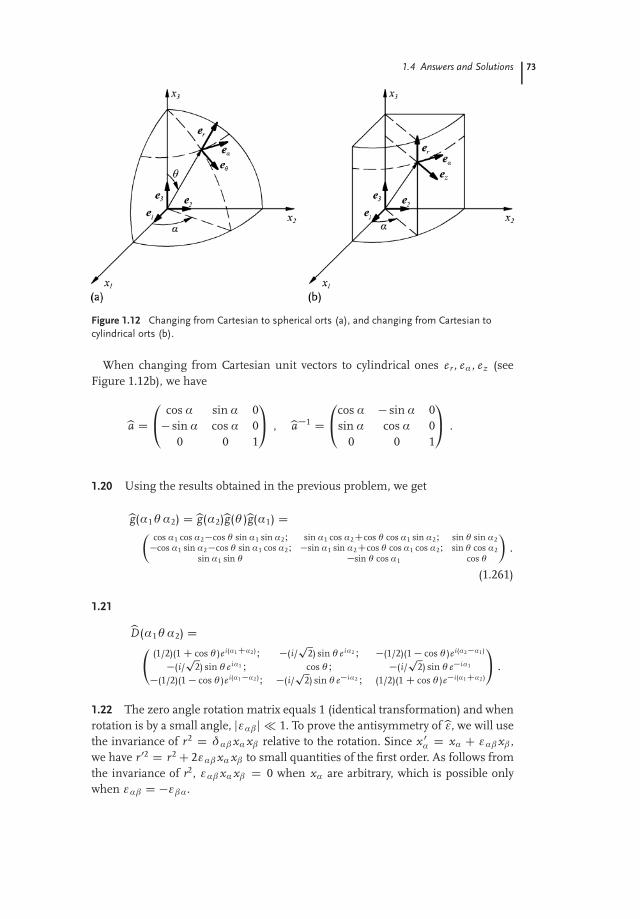
�
� Igor N. Toptygin: Foundations of Classical and Quantum Electrodynamics —Chap. c01 — 2013/10/8 — page 73 — le-tex
�
�
�
�
�
�
1.4 Answers and Solutions 73
Figure 1.12 Changing from Cartesian to spherical orts (a), and changing from Cartesian tocylindrical orts (b).
When changing from Cartesian unit vectors to cylindrical ones er , eα , ez (seeFigure 1.12b), we have
ba D0@ cos α sin α 0
� sin α cos α 00 0 1
1A , ba�1 D0@cos α � sin α 0
sin α cos α 00 0 1
1A .
1.20 Using the results obtained in the previous problem, we get
bg(α1θ α2) Dbg(α2)bg(θ )bg(α1) D�cos α1 cos α2 �cos θ sin α1 sin α2I sin α1 cos α2Ccos θ cos α1 sin α2I sin θ sin α2�cos α1 sin α2 �cos θ sin α1 cos α2I �sin α1 sin α2Ccos θ cos α1 cos α2I sin θ cos α2
sin α1 sin θ �sin θ cos α1 cos θ
�.
(1.261)
1.21
bD(α1θ α2) D (1/2)(1 C cos θ )ei(α1 Cα2)I �(i/
p2) sin θ eiα2 I �(1/2)(1 � cos θ )ei(α2 �α1)
�(i/p
2) sin θ eiα1 I cos θ I �(i/p
2) sin θ e�iα1
�(1/2)(1 � cos θ )ei(α1 �α2 )I �(i/p
2) sin θ e�iα2 I (1/2)(1 C cos θ )e�i(α1 Cα2 )
!.
1.22 The zero angle rotation matrix equals 1 (identical transformation) and whenrotation is by a small angle, jεα�j 1. To prove the antisymmetry ofbε, we will usethe invariance of r2 D δα� xα x� relative to the rotation. Since x 0
α D xα C εα� x� ,we have r 02 D r2 C 2εα� xα x� to small quantities of the first order. As follows fromthe invariance of r2, εα� xα x� D 0 when xα are arbitrary, which is possible onlywhen εα� D �ε�α.

�
� Igor N. Toptygin: Foundations of Classical and Quantum Electrodynamics —Chap. c01 — 2013/10/8 — page 74 — le-tex
�
�
�
�
�
�
74 1 The Mathematical Methods of Electrodynamics
Now, we introduce a vector with components δ'α D (1/2)eα�γ ε�γ . Then, r 0 Dr C δ' � r , which shows that δ' is the vector of an infinitely small rotation whosedirection indicates the axis of rotation and its size indicates the angle of rotation.
1.23 If rotations are specified by small vectors δ'1 and δ'2, then, after the secondrotation,
r 00 D r 0 C δ'2 � r 0 D r C (δ'1 C δ'2) � r C δ'2 � (δ'1 � r) .
The vector of the resulting rotation δ' D δ'1 C δ'2 may be introduced only if thelast member of the second order is disregarded.
In the general case, the noncommutative character of the rotation matrices isshown by expression (1.261): the completion of rotation in the sequence α2, θ , α1,inverse with respect to the matrix it is written for (1.261) corresponds to the sub-stitution α1 ! α2. In this event, the form of the matrix will change if θ ¤ 0. Thecase of θ D 0 is in keeping with rotation by angles α1 and α2 around the sameOx3 axis and such rotations are commutative.
1.24 Any tensor of rank 2 may be written as Tα� D Sα� C A α�, whereas anyHermitian tensor may be written as T h
α� D Sα� C i A α�, where Sα� and A α�
are symmetric and antisymmetric real tensors. The antisymmetric tensor A α� isequivalent to a vector (see Problem 1.10) which will not be reduced to zero by anyrotations. This is why only the real symmetric part of the any tensor of rank 2 maybe diagonalized.
1.25
Sα� D S (1)n(1)α n(1)
� C S (2)n(2)α n(2)
� C S (3)n(3)α n(3)
� . (1.262)
1.26 Computing a determinant (1.27) while keeping in mind that the principalvalues of tensor S (i) may be invariant only if such are the coefficients of an algebraiccubic equation, we find three invariants:
I1 D S11 C S22 C S33 D S (1) C S (2) C S (3), (1.263)
I2 D D11 C D22 C D33 D S (1)S (2) C S (1)S (3) C S (2)S (3), (1.264)
I3 D D D S (1)S (2)S (3) , (1.265)
where D D jbS j is the determinant of the tensor and Dα� are the algebraic cofactorsof the determinant. Expressions in the second members of the equalities followfrom Viète’s theorem37) about the connection between the coefficients of a cubicequation with its roots. The result is valid for any tensor of rank 2.
37) François Viète (1540–1603) was an French mathematician, and a lawyer by trade.

�
� Igor N. Toptygin: Foundations of Classical and Quantum Electrodynamics —Chap. c01 — 2013/10/8 — page 75 — le-tex
�
�
�
�
�
�
1.4 Answers and Solutions 75
1.27 The row and column expansions of the determinant D D jbT j are written,respectively, as
Tα� Dγ � D D δαγ , Dγ α Tγ � D D δα� ,
where Dγ α D (�1)αCγ Δγ α is an algebraic cofactor, and Δγ α is the minor deter-minant D, that is, the determinant remaining after the elimination in it of the γrow and the α column. In accordance with the results obtained in the previousproblem, since D is invariant and since δα� is a tensor, then the algebraic cofactorsDγ α also form a tensor. Relations
T �1α� D D�α
D(1.266)
form a tensor inverse to bT . To make the inverse tensor possible, it is necessary andsufficient that D D jbT j ¤ 0.
1.29
1. A2(B � C ) C (A � B)(A � C ) .2. [(A � B) � C ] � [(A0 � B0) � C 0].
1.31
(A � A0)(B � B 0)(C � C 0) C (A � B 0)(B � C 0)(C � A0)C (B � A0)(C � B0)(A � C 0) � (A � C 0)(C � A0)(B � B0)� (A � B0)(B � A0)(C � C 0) � (B � C 0)(C � B0)(A � A0) .
1.32 Now, we will present our proof for a vector and tensor of rank 2.
1. In accordance with the situation in the problem, at any rotation A0α D A α ,
that is, A0x D A x , A0
y D A y , and A0z D A z . Rotating the coordinate system
around the O z axis by angle π, we get A0x D �A x , A0
y D �A y , and A0z D A z .
These equalities are compatible with the previous ones only if A x D A y D 0.Performing rotation around the O x axis by angle π, we will similarly prove thatA z D 0, that is, vector A D 0.
2. Any tensor of rank 2 may be represented as the sum of a symmetric tensorand an antisymmetric tensor: Tα� D Sα� C A α�. An antisymmetric tensor isequivalent to a certain pseudovector and, in accordance with what was provenabove, its components do not depend on the reference frame only if they areequal to zero. So we will consider a symmetric tensor Sα�.
We will select a coordinate system where the symmetric tensor has a diagonal formS (α)δα�. If S (α) are not equal to each another, then the components of the tensordepend on the selection of the axis, that is, what digit (1, 2, or 3) denotes the selectedone. Only when S (1 D S (2) D S (3) D S do the components of the tensor S δα� notdepend on the selection of the axis.

�
� Igor N. Toptygin: Foundations of Classical and Quantum Electrodynamics —Chap. c01 — 2013/10/8 — page 76 — le-tex
�
�
�
�
�
�
76 1 The Mathematical Methods of Electrodynamics
1.33
nα D 0 , nα n� D 13
δα�, nα n� nγ D 0 ,
nα n� nγ nμ D 115
(δα� δγ ν C δαγ δ�ν C δαν δ�γ ) .
1.34
a2
3,
a � b3
,a3
,2a2
3,
2a � b3
,(a � b)(c � d) C (a � c)(b � d) C (a � d)(b � c)
15.
1.35 n2, n02, l2, n � n0, (n � n0) � l, (n � l)2, (n0 � l)2, (n � l)(n0 � l) .
1.36 n � l, n0 � l, n1 � (n2 � n3) .
1.37
1. a �α D e0
α � e� .
2. If e� D (ba�1) α� , then (ba�1) α
� D e0α � e� D aα� ¤ a �
α ; in accordance with the
definition of the inverse matrix a �α aγ
� D δγα , a α
� a�γ D δα
γ D δγα .
3. e0α D aα� e� , eα D a α
� e0� .
4. A0� D a α
� A α , A0� D a�α Aα I A α D a�
α A0� , Aα D a α
� A0� .
5. g0α� D a γ
α a μ� gγ μ , g0α� D aα
γ a�μ gγ μ , gα� D aγ
α aμ� g0
γ μ ,
gα� D a αγ a �
μ g0γ μ .
The formulas in answer 4 are generalized directly for the cases of the transfor-mation of covariant, contravariant, and mixed components of tensors of any rank.
1.38 When the systems of coordinates are inverted, the components of the vectorsof both bases change their signs: e0
α D �eα , e0α D �eα , α D 1, 2, 3.
1.39
A � B D gα� A α B� D gα� Aα B � D Aα Bα D A α B α D inv . (1.267)
dl2 D dr � dr D gα�dxαdx� D gα�dx αdx � D dx αdxα D inv . (1.268)
Note: In all cases when covariant and contravariant components do not coincide,the operation of tensor contraction must be done as a summation assumed overone upper and one lower index. Any tensor summed over two upper and two lowersymbols is not a tensor of any rank.

�
� Igor N. Toptygin: Foundations of Classical and Quantum Electrodynamics —Chap. c01 — 2013/10/8 — page 77 — le-tex
�
�
�
�
�
�
1.4 Answers and Solutions 77
1.40
Cα D pg(A� B γ � Aγ B �) , C α D (1/
pg)(A � Bγ � A γ B�) , (1.269)
where g D jbgj and numbers α, �, γ form a circular permutation 1, 2, 3.The formulas shown may be regarded as the generalization of expression (1.23)
for the case of an oblique basis. Having written (1.269) in the form of
Cα D Eα�γ A� B γ , C α D E α�γ A � Bγ , (1.270)
we find a representation for an antisymmetric tensor of rank 3 in the oblique basis:
Eα�γ D pgeα�γ , E α�γ D 1p
geα�γ , (1.271)
where eα�γ and eα�γ , related to the orthogonal basis, are similar and determinedby conditions (1.21). It is easy to verify that E α�γ is produced from Eα�γ (and viceversa) in accordance with the rule of upping and lowering indices as per (1.35).
1.41 cos θ D A α B α
(A � A� Bγ B γ )1/2 .
1.42 gμν D
eα(D )
�μ
e(D )
α
�ν, gμν D
eα
(D )
�μ e(D )
α
�ν, gμ
ν D
eα(D )
�μ e(D )
α
�ν
D δμν .
1.44
A2 D gα� Aα A� D Aα A α I cos θ D A α B α�A2B2�1/2 ,
in complete analogy with the result obtained in Problem 1.41 for an affine system.
1.45 In accordance with the common rules (1.51), we have
E μνλ D @qμ
@x α
@qν
@x �
@qλ
@x γ eα�γ ,
wherefrom the antisymmetry of E μνλ over any pair of symbols follows. This allowsus to write E α�γ D S eα�γ , where S is a certain scalar. To define it, we consider aspecial case and get
E 123 D @q1
@x α
@q2
@x �
@q3
@x γ eα�γ Dˇ̌̌̌@qλ
@x α
ˇ̌̌̌D J�1 D g�1/2 ,
where (1.39) and (1.53) are used. Therefore, S D g�1/2, and so we have obtained,in another way, the second formula (1.271).
1.46
1. dl(1) D pg11dq1, dl(2) D p
g22dq2, dl(3) D pg33dq3.

�
� Igor N. Toptygin: Foundations of Classical and Quantum Electrodynamics —Chap. c01 — 2013/10/8 — page 78 — le-tex
�
�
�
�
�
�
78 1 The Mathematical Methods of Electrodynamics
2. The covariant basis (1.46) is such a vector.3. Using the result obtained in Problem 1.44, we find
cos #12 D g12pg11g22
, cos #13 D g13pg11g33
, cos #23 D g23pg22g33
.
4. For the curvilinear coordinate system to be orthogonal, it is necessary and suf-ficient that the equalities g12 D g23 D g13 D 0 be valid in every point of space.
1.47 For a spherical system gr r D 1, g## D r2, gαα D r2 sin2 # , gr# D gr α Dg# α D 0; gr r D 1, g## D r�2, gαα D r�2 sin�2 # , gr# D gr α D g# α D 0;e r D e r D e r�, e# D r2e# D r e r , eα D r2 sin2 # eα D r sin # eα�.
For a cylindrical system gr r D gz z D 1, gαα D r2, gr α D gr z D gαz D 0; gr r Dgz z D 1, gαα D r�2, gr α D gr z D gαz D 0; e r D e r D e r�, eα D r2eα D r eα�,ez D ez D ez�.
The asterisks mark basic unit orts introduced in Problem 1.18. Covariant andcontravariant basic vectors have different dimensions and are different in length.Their lengths are, generally speaking, not unity.
1.50 R D a2
2 C ab � b3
3 .
1.52 l, l .
1.54
drA r
D r dαA α
D dzA z
,drA r
D r d#
A#
D r sin #dαA α
.
1.55 Because the gradient contains the first derivatives over the coordinates, thefollowing notation may be used:
grad(p � r)
r3D grad (p � r)
r3C (p � r)grad
1r3
.
Using the results obtained in Problems (1.52) and (1.53), we finally get the follow-ing:
grad(p � r)
r3D � 3(p � r)r
r5C p
r3.
1.56 Direct the polar axis along the vector p and project the vector E onto the ortsof spherical coordinates:
Er D 2p cos #
r3 , E# D p sin #
r3 , E' D 0 .
In spherical coordinates, vector lines are found with the following system of equa-tions:
drEr
D rd#
E#
D r sin #d'
E'
.

�
� Igor N. Toptygin: Foundations of Classical and Quantum Electrodynamics —Chap. c01 — 2013/10/8 — page 79 — le-tex
�
�
�
�
�
�
1.4 Answers and Solutions 79
The reduction of the E' component to zero means that the differential d' D 0,that is, ' D const must also become zero and, therefore, all the vector lines liewithin the planes passing through the vector p . Inserting the nonzero projectionsof H into the only remaining equation and eliminating common factors, we geta first-order differential equation with separable variables: dr/r D 2 cot #d# . Thetermwise integration of the first and second members gives ln r � ln r0 D 2 ln sin #
or r(#) D r0 sin2 # , where r0 is the constant of integration that has the meaning ofthe distance between the vector line and the origin in the plane perpendicular tothe vector p .
1.57
r˙1 D � 1p2
e˙i α�
sin #@
@rC cos #
r@
@#˙ i
r sin #
@
@α
�,
r0 D cos #@
@r� sin #
r@
@#.
1.59 3, 0, 0, 2ω.
1.60
H D 3(m � r)rr5 � m
r3 .
1.63 '0 rr , 3' C r'0, 0, l' C r(l � r) '0
r .
1.64 '(r) D constr3 .
1.65 (a � b), a � b; 4(a � r), a � r ; 0, (2' C r'0)a � r(a � r) '0r ; �2(a � r), 3(r � a).
1.66 A C (r � A0) rr , (A0 � B C A � B 0) r
r , '0r (r � A) C '
r (r � A0), '0r (r � A) C '
r (r � A0),l�rr ('0A C 'A0).
1.68 ZV
(grad ' � curl A)dV DIS
(A � grad ') � dS DIS
' curl A � dS .
1.69 aV , aV .
1.70� Use the method of the scalar multiplication of a constant vector by each ofthe integrals in question to find the following relations:I
S
n'dS DZV
grad ' dV I (1.272)

�
� Igor N. Toptygin: Foundations of Classical and Quantum Electrodynamics —Chap. c01 — 2013/10/8 — page 80 — le-tex
�
�
�
�
�
�
80 1 The Mathematical Methods of ElectrodynamicsIS
(n � A)dS DZV
curl A dV I (1.273)
IS
(n � b)AdS DZV
(b � r)A dV I (1.274)
IS
Tα� n�dS DZV
@Tα�
@x�dV . (1.275)
All these relations may be regarded as generalizations of the Gauss–Ostrogradskii theorem:I
S
n(. . . )dS DZV
r(. . . )dV , (1.276)
where the (. . . ) symbol denotes a tensor of any rank.
1.76R
S (ru � r f ) � dS .
1.81� As per the common rule (1.105), covariant divergence is expressed as fol-lows:
Γ μμα D 1
2gμλ
�@gμλ
@qα C @gαλ
@qμ � @gαμ
@qλ
�D 1
2gμλ @gμλ
@qα ,
that is,
AμIμ D @Aμ
@qμ C 12
gμλ @gμλ
@qα Aα . (1)
Now consider the determinant g D jgμνj. Its differential equals the sum of thedifferentials of all its elements multiplied by the respective algebraic cofactors:dg D D μνdgμν , where D μν D (�1)μCν Δμν , Δμν is the minor. On the other hand,the algebraic cofactors are expressed through the components of the inverse tensor,that is, gμν: D μν D ggμν (see Problem 1.27). In the end, we have
dg D ggμνdgμν , gμν @gμν
@qλD 1
g@g@qλ
.
Having inserted the latter quantity in (1), we find the expression specified in thecondition for the problem.
1.82
ΔS D 1pg
@
@qμ
�pggμν @S
@qν
�. (1.277)

�
� Igor N. Toptygin: Foundations of Classical and Quantum Electrodynamics —Chap. c01 — 2013/10/8 — page 81 — le-tex
�
�
�
�
�
�
1.4 Answers and Solutions 81
1.83
T μνIμ D 1pg
@
@qμ
�pgT μν�C Γ ν
μλ T μλ .
1.84
AμνIν D 1pg
@
@qν
�pgAμν� .
1.86
gμνIλ D gμνIλ D 0 .
1.90�
(ΔA)r D ΔA r � A r
r2� 2
r2
@A α
@α,
(ΔA)α D ΔA α � A α
r2C 2
r2
@A r
@α,
(ΔA)z D ΔA z . (1.278)
1.91�
(ΔA)r D ΔA r � 2r2 A r � 2
r2 sin #
@
@#(A# sin #) � 2
r2 sin #
@A α
@α,
(ΔA)# D ΔA# � A#
r2 sin2 #C 2
r2
@A r
@#� 2 cos #
r2 sin2 #
@A α
@α,
(ΔA)α D ΔA α � A α
r2 sin2 #C 2
r2 sin #
@A r
@αC 2 cos #
r2 sin2 #
@A#
@α. (1.279)
1.92 (i) A C B ln r ; (ii) A C B α; (iii) A C B z.
1.93 (i) A C Br ; (ii) A C B ln tan( #
2 ); (iii) A C B α.
1.94�
x D ˙�
(� C a2)(η C a2)(� C a2)(b2 � a2)(c2 � a2)
�1/2
,
y D ˙�
(� C b2)(η C b2)(� C b2)(c2 � b2)(a2 � b2)
�1/2
,
z D ˙�
(� C c2)(η C c2)(� C c2)(a2 � c2)(b2 � c2)
�1/2
I
h1 Dp
(� � η)(� � � )2R�
, h2 Dp
(η � � )(η � � )2Rη
,

�
� Igor N. Toptygin: Foundations of Classical and Quantum Electrodynamics —Chap. c01 — 2013/10/8 — page 82 — le-tex
�
�
�
�
�
�
82 1 The Mathematical Methods of Electrodynamics
h3 Dp
(� � � )(� � η)2R�
I
Δ D 4(� � η)(� � � )(η � � )
�(η � � )R�
@
@�
�R�
@
@�
�
C(� � � )Rη@
@η
�Rη
@
@η
�C (� � η)R�
@
@�
�R�
@
@�
��,
where Ru D p(u C a2)(u C b2)(u C c2). The formulas for x, y, and z show that
there are eight threes: x , y , z for every three values of � , η, � . One may makesure that the ellipsoidal system of coordinates is orthogonal by finding gradientsr� , rη, r� and then the scalar products r� � rη and so on, all of which turn outto be equal to zero. The gradients may be found directly from the equations deter-mining ellipsoidal coordinates (see the condition for the problem), resulting in agradient from both members of each of these equations.
1.95�
z D ˙�
(� C c2)(η C c2)c2 � a2
�1/2
, r D�
(� C a2)(η C a2)a2 � c2
�1/2
I
h1 Dp
� � η2R�
, h2 Dp
� � η2Rη
, h3 D r ,
where
R� Dq
(� C a2)(� C c2) , Rη Dq
(η C a2)(�η � c2) I
Δ D 4� � η
�R�
@
@�
�R�
@
@�
�C Rη
@
@η
�Rη
@
@η
��C 1
r2
@2
@α2 .
1.96�
x D ˙�
(� C a2)(� C a2)a2 � b2
�1/2
, r D�
(� C b2)(� C b2)b2 � a2
�1/2
I
h1 Dp
� � �2R�
, h2 D r , h3 Dp
� � �2R�
,
where
R� Dq
(� C a2)(� C b2) , R� Dq
(� C a2)(�� � b2) I
Δ D 4� � �
�R�
@
@�
�R�
@
@�
�C R�
@
@�
�R�
@
@�
��C 1
r2
@2
@α2.

�
� Igor N. Toptygin: Foundations of Classical and Quantum Electrodynamics —Chap. c01 — 2013/10/8 — page 83 — le-tex
�
�
�
�
�
�
1.4 Answers and Solutions 83
1.97�
h� D hη D acosh � � cos η
, hα D a sin ηcosh � � cos η
I
Δ D (cosh � � cos η)3
a2
�@
@�
�1
cosh � � cos η@
@�
�
C 1sin η
@
@η
�sin η
cosh � � cos η@
@η
�
C 1
sin2 η(cosh � � cos η)
@2
@α2
�.
1.98� The surfaces � D const are toroids:
(q
x2 C y 2 � a coth �)2 C z2 D�
asinh �
�2
I
the surfaces � D const are spherical segments:
(z � arctan � )2 C x2 C y 2 D�
asin �
�2
I
h� D h� D acosh � � cos �
, hα D a sinh �
cosh � � cos �.
1.99 x ν Zν (x ) C C , �x�ν Zν(x ) C C .
1.100 1, 12 , 1
2n n! .
1.107�
1. x u00 C u0 C x (a2 � n2
x2 )u D 0 .2. The integral is computed with the use of the equations for the functions u(x )
and v (x ) D Jn(bx ).3. The first equality (1.175) directly follows from (1.174); the second one results
from passage to the limit.
1.111
P0 D 1 , P1 D x , P2 D 12
(3x2 � 1) , P3 D 12
(5x3 � 3x ) ,
P4 D 18
(35x4 � 30x2 C 3) , P5 D 18
(63x5 � 70x3 C 15x ) .

�
� Igor N. Toptygin: Foundations of Classical and Quantum Electrodynamics —Chap. c01 — 2013/10/8 — page 84 — le-tex
�
�
�
�
�
�
84 1 The Mathematical Methods of Electrodynamics
1.112� The integral that should be computed contains the product of the deriva-tives
R 1�1[(x2 � 1)l ](l)[(x2 � 1)l 0 ](l
0)dx . To make things clear, l 0 l . Integrating byparts, l times, we find (�1)l
R 1�1(x2 � 1)l [(x2 � 1)l 0 ](lCl 0)dx . The second factor un-
der the integral is other than zero only when l 0 D l . In this case, beginning byintegrating over the angle # , we get
1Z�1
(x2 � 1)l [(x2 � 1)l ](2l)dx D (�1)l(2l)!2
π/2Z0
(sin #)2lC1d#
D (�1)l(2l)!B�
l C 1,12
�.
The last integral here is expressed through a beta function (see the definition inAbramovitz and Stegun, 1965; Gradshtein and Ryzhik, 2007):
B(z, w ) � Γ (z)Γ (w )Γ (z C w )
D 2
π/2Z0
(sin #)2z�1(cos #)2w�1d# .
Carefully eliminating factorials and gamma functions, we get the result specifiedin the condition for the problem.
1.114 P2 D 1C3 cos 2#4 .
1.115
1sin #
dd#
sin #dP m
l
d#C�
l(l C 1) � m2
sin2 #
�P m
l D 0 .
1.116� Use the Leibniz formula to find
(1 � x2)m/2[(x C 1)l (x � 1)l ](lCm)
D (�1)m/2lCmXkD0
(l C m)!l !l !k!(l C m � k)!(k � m)!(l � k)!
(x C 1)k�m/2(x � 1)l�kCm/2 I
and
(1 � x2)�m/2[(x C 1)l (x � 1)l ](l�m)
D (�1)�m/2l�mXsD0
(l � m)!l !l !s!(l � m � s)!(s C m)!(l � s)!
(x C 1)sCm/2(x � 1)l�s�m/2 .
In both sums, the limits of summation are, actually, determined by the presence inthe denominators of the factorials of negative integers. In the second sum, replacethe summation index s ! k�m. As a result, in both sums, factors that depend on kbecome the same. Comparing them with each other, we find the formula specifiedin the condition for the problem.

�
� Igor N. Toptygin: Foundations of Classical and Quantum Electrodynamics —Chap. c01 — 2013/10/8 — page 85 — le-tex
�
�
�
�
�
�
1.4 Answers and Solutions 85
1.117
P0l D Pl ,
P11 D �2P�1
1 D (1 � x2)1/2 D sin #,
P12 D �6P�1
2 D 3x (1 � x2)1/2 D 3 cos # sin #,
P22 D 24P�2
2 D 3(1 � x2) D 3 sin2 #,
P13 D �12P�1
3 D 32
(5x2 � 1)(1 � x2)1/2 D 32
(5 cos2 # � 1) sin #,
P23 D 120P�2
3 D 15x (1 � x2) D 15 cos # sin2 #,
P33 D �720P�3
3 D 15(1 � x2)3/2 D 15 sin3 # .
In the general case, adjoint Legendre polynomials contain radicals (1 � x2)1/2 and,therefore, strictly speaking, are not polynomials.
1.118� When computing the normalization integral, use formula (1.198) and themethod used to solve Problem 1.112�:
1Z�1
[P ml (x )]2dx D (�1)m (l C m)!
(l � m)!
1Z�1
P ml (x )P�m
l (x )dx
D (2l)!(l C m)!22l l !l !(l � m)!
B(l C 1, 1/2) ,
Cl m Ds
2l C 14π
(l � m)!(l C m)!
.
Expressing the beta function through gamma functions and reducing fractions, wefind the normalization factor (down to the phase factor over the module equaling1, which remains arbitrary).) In the end, we get the normalized spherical Legendrefunction:
Yl m(#, ')
Ds
2l C 14π
(l � m)!(l C m)!
(1 � cos2 #)m/2�
dd cos #
�lCm
(cos2 # � 1)l e i m' .
1.119
1sin #
@
@#sin #
@Yl m
@#C 1
sin2 #
@2Yl m
@'2C l(l C 1)Yl m D 0 .
1.120 � 53 , �2 , 0 , exp(α) C exp(�2α) .

�
� Igor N. Toptygin: Foundations of Classical and Quantum Electrodynamics —Chap. c01 — 2013/10/8 — page 86 — le-tex
�
�
�
�
�
�
86 1 The Mathematical Methods of Electrodynamics
1.121 0 , f (a)δ(x � a) , 82δ(x � 4) C 2δ(x C 1) .
1.123
δ(r) D 12π r?
δ(r?)δ(z) ,
δ(r � a) D 1a?
δ(r? � a?)δ(α � α0)δ(z � az ) .
To achieve passage to the limit a ! 0, one must not only make values a? and az
tend to zero, but must also average the second member over the azimuthal angleα0, since a zero vector has no direction.
1.124
δ(r) D 14π r2 δ(r) , δ(r � a) D 1
a2 δ(r � a)δ(cos # � cos #0)δ(α � α0) .
1.125
f 0(x ) D g(x ) C 2δ(x � 1) , where g(x ) D(
3x2 , if x < 1 ,
2x , if x > 1 .
1.126
f 0(x ) D d fdx
CnX
kD1
Δ f k δ(x � ak ) ,
where Δ f k D f (ak C 0) � f (ak � 0), d f /dx is a proper (“classical”) derivative inthe areas of the smooth variation of the function.
1.127
(�1)m m!(n � m)!
f (m�n)(0) at m � n , 0 at m < n .
1.128 When r ¤ r 0, G is a bounded differentiable function and the equation issatisfied, since ΔG D 0. When r ! r 0, the function has a singularity. To find outthe nature of that singularity ΔG when r ! r 0, integrate (1.225) over the volumeof a small sphere of radius R ! 0 with its center at the point r D r 0. Using theGauss–Ostrogradskii theorem, we getZ
V
ΔGdV DZV
div grad�
1r
�dV D
IS
�r 1
r
�� dS
D �Z
1R2 R2dΩ D �4π .
The same value is obtained by the integral over the volume in the second memberof the equation, which is how it is satisfied.
�
� Igor N. Toptygin: Foundations of Classical and Quantum Electrodynamics —Chap. c01 — 2013/10/8 — page 87 — le-tex
�
�
�
�
�
�
1.4 Answers and Solutions 87
1.129
f (x ) D π2
� 4π
1XkD0
cos(2k C 1)x(2k C 1)2
.
1.130
f (x ) D 4aπ
1XkD0
sin(2k C 1)x2k C 1
.
1.131
f (x ) D a2
C 2aπ
1XkD0
(�1)k cos((2k C 1)πx/L)2k C 1
.
The Fourier series of f (�x ) D f (x ), which is a function that is even within theinterval [�L, CL], contains only cosines. The odd function f (�x ) D � f (x ) is ex-pandable in sines. A function that has no clear-cut parity contains both sines andcosines in its Fourier expansion.
1.132 i λF(λ).
1.133
1a
F�
λ � ba
�.
1.134 π exp(�jλj).
1.135 pπ
αexp
�� λ2
4α2
�.
1.136
π3/2
α3 exp�
� k2
4α2
�,
where k is a radius vector of the three-dimensional space of Fourier variables (see(1.252)).
1.137� 4πk2C�2 .
1.138� To compute Fourier integral (1.252), use spherical coordinates and selectthe O z axis along the vector k. Firstly, doing integration over angles and then over r,we find
F(k) D limR!1
4πk2 [1 � cos(k R)] .

�
� Igor N. Toptygin: Foundations of Classical and Quantum Electrodynamics —Chap. c01 — 2013/10/8 — page 88 — le-tex
�
�
�
�
�
�
88 1 The Mathematical Methods of Electrodynamics
Formally, the function in the second member has no limit. However, it is easyto understand that the limit of the cosine may be regarded as effectively equal tozero since, when the inverted Fourier transformation is being done, the memberwith infinitely oscillating cosine will make zero contribution. As a result, we haveF(k) D 4π/ k2.
1.139 Write down the expansion as
exp(i k r cos θ ) D1X
lD0
u l(k r)Pl(cos θ )
and, using the orthogonality of Legendre polynomials (see Problem 1.112�), findan integral representation of the functions ul sought:
u l(k r) D 2l C 12
1Z�1
e i k r x Pl (x )dx .
Use the Rodrigues formula and integrate l times by parts to get
u l(k r) D (2l C 1)(�i k r)l
2lC1 l !
1Z�1
e i k r x(x2 � 1)ldx .
Further, expand the exponent in a power series and integrate this absolutely con-vergent series termwise. Only terms with even powers of x are left:
u l(k r) D (2l C 1)(�i k r)l
2l l !
1XmD0
(i k r)2m
(2m)!
1Z0
x2m(x2 � 1)ldx .
Finally, the transition to a new integration variable t D x2, dx D dt/2p
t allowsus to express the integral in the latter equality through a beta function:
1Z0
t k�1/2(1 � t)l d t D B(k C 1/2, l C 1) D Γ (k C 1/2)Γ (l C 1)Γ (l C k C 3/2)
.
In the end, bundle all the factors to get the following series:
u l(k r) D i l(2l C 1)(k r)l
1 � 3 . . . (2l C 1)
��
1 � k2r2/21!(2l C 3)
C (k2r2/2)2
2!(2l C 3)(2l C 5)� . . .
D i l(2l C 1) j l(k r) ,

�
� Igor N. Toptygin: Foundations of Classical and Quantum Electrodynamics —Chap. c01 — 2013/10/8 — page 89 — le-tex
�
�
�
�
�
�
1.4 Answers and Solutions 89
where j l(k r) is a spherical Bessel function; see formulas (10.1.2) in Abramovitzand Stegun (1965).
1.140�
exp(i k � r) D 4π1X
lD0
lXmD�l
i l j l(k r)Y �l m(θ , φ)Yl m(#, ') .

�
� Igor N. Toptygin: Foundations of Classical and Quantum Electrodynamics —Chap. c02 — 2013/10/8 — page 90 — le-tex
�
�
�
�
�
�