1. the wave function, s.e. and basic operators · 2010. 8. 29. · operators, expectation values...

1. The Wave Function, S.E. and Basic Operators

Background

The SP351 handout: Definite Integrals for Quantum Mechanics

Complete course covering modern physics

A course in intermediate mechanics

Harris, Non-Classical Physics

Paul A. Tipler, Ralph A. Llewellyn, Modern Physics

Concepts of primary interest:

Born Interpretation

Copenhagen Interpretation

Schrödinger equation

Operators, expectation values and commutators

Ehrenfest’s theorem

Sample calculations:

Helpful handouts:

Definite integrals

Tools of the trade:

The probability current J(x,t) is real; reduces the work by half!

Appendix:

Postulates of Quantum Mechanics

Many thoughts are presented a large number of times in these guides. Do not ignore

the repetitions. Each time you encounter one, ask yourself if you understand it and the

reason that the thought is worth repeating.

Quantum mechanics is a strange and difficult field. The plan is to learn to extract

values from the formalism of quantum mechanics rather than to discuss its philosophy

or its possible variants (with or without hidden variables). The Copenhagen view is to

be adopted. Students should memorize definitions and careful statements of the

for use with Griffiths QM Contact: [email protected]

principles as outlined. Wait at least another semester before becoming side-tracked by

other interpretations or philosophies.

Rather than state a leanest set of postulates to serve as a basis for quantum mechanics,

a larger set of known facts is to be presented. This approach requires fewer

mathematical steps to compute meaningful results.

This handout is written with the assumption that you have completed a one year study

of modern and atomic physics and that you are familiar with the standard results for

free particles, barriers, wells, oscillators and the hydrogen atom. These handouts are to

be used with Griffiths Quantum Mechanics, not as a stand-alone reference.

The wave function: A quantum system is described by a wave function which

contains all the information that can be known about the system. It is a function of the

generalized coordinates for the system and time. In 1D, the function might have the

form (x,t). It is a complex-valued function. (Later, the function is to be generalized to

a KET in an abstract vector space.)

Born’s statistical interpretation of the wave function is that * ( , ) ( , )b

ax t x t d x

represents the probability to find the particle described by the wave function in the

interval [a, b]. That is: (x, t)(x, t) is the probability density (x). The total

probability should by one so our standard normalization condition is to be:

* ( , ) ( , ) 1fullrange

x t x t dx [WF.1]

8/29/2010 SP425 Notes – Wave Functions, Schrödinger and Operators Ch1-2

Time Development: Schrödinger proposed the equation that governs the time-

development of the wave function.1

2 2

2ˆ( , ) ( , ) ( ) ( , )

2i x t H x t V x x

t m x

t [WF.2]

The Schrödinger Equation (SE)

The operator 2 2

2( )

2V x

m x

is a sample hamiltonian for a one dimensional

system. At least in simple cases, the hamiltonian represents the energy of the system.

Expressing [WF.2] as an eigenvalue equation leads to the time-independent

Schrödinger’s equation.

2 2

2( ) ( , ) ( , ) ( , )

2 n n n nV x x t E x t i x tm x t

[WF.3]

First the separation hypothesis is invoked. Assume: n(x,t) = un(x) Tn(t).

Time independent SE: 2 2

2( ) ( ) ( )

2 n n nV x u x E u xm x

[WF.3a]

Time dependence: ( ) ( )n n nE T t i T tt

( )

En

n

iT t e

t

[WF.3b]

Time dependence of energy eigenfunctions: n(x,t) = un(x) Enie t

[WF.3c]

In summary, the hamiltonian is the time development operator for the wave function,

and it is the energy operator for most systems (essentially for all systems that we shall

study).

1 See the article by Felix Bloch in the December 1976 issue of Physics Today.


Erwin Rudolf Josef Alexander Schrödinger (August 12, 1887 – January 4, 1961) was an Austrian - Irish physicist who achieved fame for his contributions to quantum mechanics, especially the Schrödinger equation, for which he received the Nobel Prize in 1933. In 1935, after extensive correspondence with personal friend Albert Einstein, he proposed the Schrödinger's cat thought experiment. On January 4, 1961, Schrödinger died in Vienna of tuberculosis at the age of 73. The huge Schrödinger crater on the far side of the Moon was posthumously named after him by the IAU. The Erwin Schrödinger International Institute for Mathematical Physics was established in Vienna in 1993. http://en.wikipedia.org/wiki/Schroedinger

= h/2 = 1.05457 x 10-34 Js = 4.1357 x 10-15 eV s

Is the normalization preserved in time?

( ) * ( , ) ( , )fullrange

N t x t x t dx ; (N(to) = 1),

If the wavefunction is normalized at time to, does it remain normalized for later times?

That is: does dN/dt = 0?

*( , ) ( , )* ( , ) ( , ) ( , ) * ( , )full full

x t x tdN dt tdt dt x t x t dx x t x t d x [WF.4]

Use the Schrödinger’s equation to evaluate the time derivatives:

2

2

1( , ) ( ) ( , )

2

ix t V x

t m x i

x t [WF.5]

2

2

1( , ) ( ) ( , )

2

ix t V x

t m x i

x t [WF.6]

After substituting and combining terms,

2 2

2 2

*( , ) ( , )2* ( , ) ( , ) ( , ) * ( , )full full

range rangex x

x t x td imdt x t x t dx x t x t d

x

Use: 2 2

2 2

*( , ) ( , ) ( , ) ( , )( , ) * ( , ) * ( , ) ( , )x xx x xx t x t x tx t x t x t x t

x t

Assigning and u as the lower and upper limits of integration for definiteness,

2

( , ) ( , )* ( , ) ( , ) * ( , ) ( , ) 0uu

x xi

m

x t x tddt x t x t dx x t x t

[WF.7]


It will be shown that the wavefunction vanishes at the limits or that () = (u) for all

problems of interest to us. In the particular case of limits must vanish at the

limits or the function cannot be normalized. It follows that dN/dt = 0.

In any of these cases, it follows that the normalization integral is time-

independent. Once a wave function is normalized, it will remain normalized.1

Probability current: The probability Pab to find the particle between a and b is

* ( , ) ( , )b

ax t x t d x . While * ( , ) ( , ) 1full

range

x t x t dx , a constant, Pab can vary in

time. The range limits a and b are fixed values.

*( , ) ( , )* ( , ) ( , ) ( , ) * ( , )abb b

a a

x t x tdP dt tdt dt x t x t dx x t x t dx

Define J(x, t) as the probability current in the +x direction. ( , ) ( , )abdPdt J a t J b t

Using Schrödinger’s equation, 2 2

2( , ) ( ) ( , )

2i x t V x x

t m x

t and its

complex conjugate, the time-dependence, after the terms in V(x) cancel, is:

2 2

2 2

*( , ) ( , )2 2( , ) * ( , )ab

b

a x xx t x tdP i i

m mdt x t x t

dx

*( , ) ( , )2 ( , ) * ( , )ab

b

a x x xx t x tdP i

mdt x t x t dx

*( , ) ( , )2 ( , ) * ( , ) ( , ) ( , )

b

ax xx t x ti

m x t x t J a t

J b t

1 See Griffiths problem 1.15 which demonstrates the behavior of the normalization for a system with a non-Hermitian

hamiltonian. Complex potentials can be used to model particle absorption or decay.


Recall: J(x,t) represents the probability current in the positive direction at x. The rate of

change of Pab is + J(a,t) - J(b,t), the flow in at the small x boundary minus the flow out

at the large x boundary. Comparing, the probability current is identified as:

Probability current: J(x,t) = *2 *x xim

[WF.8]

Exercise: Compute the probability currents for a plane wave [i kx tAe ] , for the mixed

oscillator state 10 12

[ ] and for the mixed box state 42[sin( ) sin( ) ]it itx xa aA e e for

(0 < x < a).

Exercise: Show that the probability current is real.

Exercise: Prepare a sketch and justify the identification:

* ( , )b

a

ddt dx J b t J a t ( , ) .

A first expectation value:

In as much as the probability density is (x) = (x,t)(x,t), the expectation value of x

can be computed as:

( ) * ( , ) ( , ) * ( , ) ( , )full full fullrange range range

x x dx x x t x t dx x t x x t dx

*( , ) ( , )fullrange

x x t x x t dx [WF.9]

The point of the rightmost version is that x could equally well be sandwiched between

and . The sandwiched position is to be our standard position for operators.

Sample Calculation: Expectation value of x in a box (infinite well) state.

Given (x) = A sin[ x/a] for 0 < x < a; (x) = A sin[

x/a] = 0 otherwise.


1.) Normalize the wavefunction. 20

[ sin( )]* sin( ) * ( ) 1a

x xa a

aA A dx A A .

0

2* *2 21 (1 cos( )

ax

aA A A Adx a ( )

It follows that |A|2 = 2/a. The spatial part of the wavefunction can be assumed to be real

if the hamiltonian is real. We conclude that 2( ) sin( )xa ax .

2.) Compute the expectation value of x. 0

2 2[ sin( )]* sin( )a

x xa a a ax x d x .

0 0

2 21 12(1 cos( ) cos( )

a ax x

a aa

a ax x dx x dx

The remaining integral on the right yields to integration by parts. It vanishes.

x = ½ a

Discussion: The result is not surprising as the probability density for all the infinite

well states is symmetric about the center of the well. It follows that xis the position

of the well center for a infinite square well with a flat bottom.

Exercise: Evaluate 0

2cos( )a

xax dx .

Exercise: Show that: 2[sin( )]m xa

is even about ½ a. Define = x - ½ a. Use one of

our favorite identities, 2 sin2 = 1 – cos(2).

Plot illustrating the decomposition of sin[x] x sin[x] into sin[x] (½)sin[x] + sin[x] (x - ½) sin[x] Note that the wavefunction is not normalized. The plot still establishes that:

1 12 2

0 0sin[ ] sin[ ] ½ sin[ ] sin[ ]A x x x dx A x x dx


Motivating the momentum operator: The operator for position x was introduced

without comment; it was the obvious choice. It is not obvious how momentum

information is to be extracted from a wave function and its associated probability

density as they are functions of position (x) and time (t). As a first step, one could

study the time dependence of the of the expectation value of the position:x

*( , ) ( , )* ( , ) ( , ) ( , ) * ( , )full fullrange range

x t x td dt tdt dtx x t x x t dx x x t x t x dx

Note that the integrals are over the full range of the coordinates and are therefore the

limits of integration are time-independent. The time derivative of the wave function

can be computed using the Schrödinger equation. Substituting from [WF.5] and

[WF.6], and then using the identity above [WF.7], it follows that:1

( , ) ( , )* ( , ) ( , )2 full

rangex x x

x t x tddt

ix x x t x t

m

dx

This expression is integrated by parts, and the surface terms evaluated to be zero as

before.

( , ) ( , )* ( , ) ( , )2 full

rangex xx t x td

dti

x x t x t dxm

Next, the second term is integrated by parts, and the surface terms evaluated as zero.

( , )* ( , )fullrange

xx td

dti

x x t dxm

Multiplying by m to get to momentum, and relocating the operator parts in the

sandwiched position,

* ( , )( ) ( , )fullrange

xddtp m x x t i x t d

x [WF.10]

1 One should review Leibnitz rule [WF.24] for this derivative and then review the time invariance of the normalization.


The result suggests that: ˆ x xp i is the operator for the x component of

momentum.1 We use it to extract information about the system’s momentum from the

wave function which contains all the information that can be known about the system.

See problem 1 in this summary for an additional motivation for this identification.

The transition from classical mechanics to quantum mechanics: There are several

formulations of classical mechanics. Newtonian mechanics is studied first and then

Lagrangian mechanics. Hamiltonian mechanics is developed from the Lagrangian

form. That Hamiltonian form leads directly to the Poisson bracket form. The transition

to quantum mechanics is probably most natural if made from the Poisson bracket

formulation of mechanics, but only a familiarity with the Lagrangian and Hamiltonian

forms is to be the assumed basis for these discussions.2 It is recommended that you

reconsider the transition to quantum mechanics after you study the Poisson bracket and

action-angle formulations of mechanics.3

For now, the important point is that the hamiltonian and any other dynamical quantity

are considered to be functions of the generalized coordinates, the conjugate

generalized momenta and time. In the cases in which the Hamiltonian is time

independent, it is the energy of the system.

( , , )i iQ q p t

What is an operator? An operator is a mapping that acts on a wavefunction (for the

problem) and returns a wavefunction (or a constant times a normalizable

wavefunction) for that same problem.4 One might consider the energy eigenstates of a

1 The argument used to motivate the form of the operator for momentum is actually a circular argument! 2 A very basic review of Lagrangian and Hamiltonian mechanics is included just before the problem section. 3 Action-angle mechanics is the most natural basis for the Bohr and Bohr-Sommerfeld models of atoms. 4 Linear Vector Spaces: An operator acts on a vector in a space to return a vector in the same space.


harmonic oscillator, {… , n(x,t), … }. For example, the multiplication by x operation

executed at time tM returns a mixed state.

0 0

14

1 1

2

21

2( , ) ( , ) ( , )M Mi t i tn M n M n M

n nmkx x t e x t e x t

The result is a permissible state of the oscillator, but it is neither normalized nor is it an

energy eigenstate. Further one could argue that the result does not have the dimensions

of a wave function. This flaw is not an issue as the normalization process restores the

correct dimensions: in the Schrödinger picture [pure density]½ or [length]-D/2 where

D is the spatial dimensionality. One might just declare that all wavefunctions that are

constant multiples of one another are the same. By analogy, the wavefunction is a

vector in a complex space of high dimension, and the quantum state is specified by the

direction (sans magnitude) of that vector.

Exercise: Carefully analyze the dimensions wavefunctions for the n = 0 state of the

QHO and for the 1S state electron in hydrogen. Do the dimensions agree with your

expectations? Recall that * is a probability density. * d = 1 where d is dx for

the oscillator and dV for the hydrogen atom.

The operator postulate: In our standard coordinate representation, the quantum

operator for the momentum conjugate to the generalized coordinate qi is iqi

, and

the operator for the dynamical quantity is: ( , , )i iQ q p t

ˆ ˆ ˆ( , , ) ( , , )i i i iqQ q p t Q q i t [WF.11].

There will be some fine tuning as, in quantum mechanics, the order matters. Products

of operators are to be replaced by averages of the operators over all re-orderings. For

example, the dynamical quantity x px is to be rewritten as ½ [ x px + px x] leading to:


ˆ ˆ ˆ ˆ½ ½x x x x xx p x p p x i x x

The expectation value of the dynamical quantity is to be computed as: ( , , )i iQ q p t

ˆ ( , , ) ( , ) ( , , ) ( , )i i i i iiqQ q p t q t Q q i t q t d [WF.12]

The integration is to be carried out over the full ranges of the generalized coordinates,

and d represents the generalized volume element associated with the generalized

coordinates.

ˆ ( , ) ( , , ) ( , )i i iiqQ q t Q q i t q t d

The expectation value of . ˆ ( , , )i iQ q p t

Given an eigenstate: ˆ ( , ) ( , )n nn

tH x t E x t i and

ˆ0Q

t then:

. ˆ ( , ) ( , ) ( , ) ( , ) 0i i i i iiqd ddt dtQ q p q t Q q i q t d

ˆ ( , ) ( , ) ( , ) 0i i i ii iq qt tddt Q q p Q q i Q q i d

*ˆ ( , ) ( ) ( , ) ( , ) 0i i n i i ni iq qiQ q p E Q q i Q q i E d

The expectation value of a time-independent operator is a constant for any the state

is an energy eigenfunction (stationary state).

Exercise: Compute x for the SHO state: 012

12( , ) ( , )1x t x t . Show that it is time

dependent. This result does not conflict with the statement that appears just before this

exercise. Explain.

Exercise: A particle moves in one dimension under the influence of a potential V(x).

Its kinetic energy is . Give the form of the Lagrangian L(x, 2½ m x x ). Compute the


generalized momentum px = Lx conjugate to x. Deduce an expression for the total

mechanical energy. Express that energy as a function of x and px.

Exercise: A particle moves in one dimension under the influence of a potential V(x).

Its kinetic energy is . It has the hamiltonian H(x,px) = (1/2m) px2 + V(x). 2½ m x

Construct the quantum operator that represents this Hamiltonian function.

Hermitian property of operators and measurements: If an operator corresponds to a

quantity that can be measured, its expectation values and eigenvalues must be real.

Hermitian operators meet this requirement. An operator is Hermitian if:

ˆ ˆ( , ) ( , ) ( , ) ( , ) ,i i i iq t Q q t d Q q t q t d

The functions (qi,t) and (qi,t) are any permissible wavefunctions for the problem.

The requirements to be permissible may be that the wavefunction have a finite

normalization and that it satisfies the characteristic boundary conditions of the

problem. For example, infinite square well wavefunctions must vanish at the edges of

the well. Examples of our common Hermitian operators include the hamiltonian, the

position operator x and the momentum operator, - xi .

Measurements in quantum mechanics: A measurement is an operation that returns a

precise value for some dynamical quantity. A measurement must return a real value,

and each quantity that can be measured has an associated Hermitian operator . Q

Every Hermitian operator has a complete set of eigenfunctions (which can be chosen to

be mutually orthogonal; Gram-Schmidt) with corresponding real eigenvalues. (For the


hydrogen atom problem, the hamiltonian, the square of the orbital angular momentum

and the operator for the z component of angular momentum each have a complete set

of eigenfunctions. There are cases in which the operators can share the same complete

set of eigenfunctions and cases for which they cannot. In the case of hydrogen, the

operators listed ( 2ˆ ˆ ˆ, ,H L L ) are said to commute, and all three can share the same set of

eigenfunctions.) Operators commute if making the measurement associates with one of

the operators does not disturb the measured value corresponding to the other operator.

Eigenvalue equation: ˆ ( , ) ( , )n n nQ x t q x t

Completeness: any general ( , ) ( , )n nall n

x t a x t

and 2| ( , ) ( , )| 0N

n nfullN range n start

Lim x t a x t dx

The equation just above is the requirement for completeness: that the expansion in

terms of eigenfunctions converges in the mean to the function. We conclude that the

sum faithfully represents the function (x,t) without missing anything

important.

( , )n nall n

a x t

Mathspeak, fuzzy: Quantum mechanics lives in Hilbert space which is a space of general

function vectors that contains the limit vector of all the sequences of vectors in that space. A

sequence with members Sn(x,t) = leads to the limit vector up to

( , )n

m mm

a x t t( , )n nall n

a x

which itself is a vector in the space. This statement applies for normalizable vectors only.

This statement also fails the math purity test. It is only provides a hint as to why the term

Hilbert is added to space for applications to quantum mechanics. At the graduate level, one

should revisit the terms Hermitian and self-adjoint for finite and infinite dimensional spaces.


General Time Dependence: Eigenfunctions of the hamiltonian play a

special role in part because they have a separable time dependence and

hence stationary probability densities.

Eigenvalue equation: ˆ ( , ) ( , )n n nH x t E x t

1where( , ) ( ) nn n n

i tnx t x e E and ˆ ( , ) ( , )n n nH x t E x t

Any function can be expanded in terms of the n(x) at an initial time to.

0 0( , ) ( ) ( )n nall n

x t a t x

00

( )( , ) ( ) ( ) nn n

all n

i t tx t a t x e The wave function at any time t is .

1.) The Collapse Postulate: Any precise measurement collapses the wave function to

one that is consistent with the measured value. If the measurement is repeated

immediately, the same value will be found. The state evolves in time as directed by the

hamiltonian, and a measurement repeated after some time has elapsed does not

necessarily yield the same result. Even a very rapid sequence of measurements of the

position, then momentum and then position again can yield initial and final position

values that are essentially unrelated. The x position and x component of momentum are

examples conjugate quantities. A measurement of one of the quantities disturbs the

value of the other.

We may think of the measurement as adding a term to the hamiltonian for the duration

of the measurement. This new term can be large, and it causes the peculiar collapse of

the wave function in short order.

The measurement operator has a complete set of eigenfunctions n(x,t) so the pre-

measurement wavefunction (x,t) can expended in terms of them.


(x,t) = a 1(x,t) + b 3(x,t)+ c 7(x,t) + d 8(x,t) + f 10(x,t),

If only and have the eigenvalue measured, then, when an ideal measurement of

the quantity is made and the eigenvalue consistent with and is found, the state is

collapsed to:

3 8

2 2

( , ) ( , )( , )

| | | |

b x t d x tx t

b d

[WF.13]

All the inconsistent terms are eliminated, and the consistent terms survive including

their associated phase information. The state immediately after the measurement is the

normalized function [WF.13].

2.) The expectation value for a measurement can be computed as:

ˆ* ( , ) ( , )fullrange

Q x t Q x t dx

The expectation value is the average of the values of measurements on an ensemble of

systems all prepared according to the same recipe (x,t). The expectation value is the

average of the first measurements over an ensemble of identically prepared systems; it

is not the average of repeated measurements on the same system.

Exercise: Discuss the necessity to make first measurements on an ensemble rather than

repeated measurements on a single system in light of the collapse postulate.

3.) Expansions in terms of the eigenfunctions of the measurement operator:

Given that: and ˆ ( , ) ( , )n n nQ x t q x t ( , ) ( , )n nall n

x t a x t , and one concludes that:


Q x t Q x t dx 2| |nall n

a q n = [WF.14]


and that |an|2 is the probability that a system described by (x,t) return the eigenvalue

corresponding to the state n(x,t). This statement assumes that the eigenvalues are not

degenerate. Take a moment to consider the complications that arise when several of the

eigenfunctions have the same eigenvalue qm.

Further, one can measure the expectation value of any power of Q.

ˆ* ( , )[ ] ( , )m mfullrange

Q x t Q x mt dx 2| | ( )mn n

all n

a q =

At this point we tip our hats to the mathematicians who have proven that this outcome

is possible only if the eigenvalues {... , qi, …} are the only possible outcomes of a

precise measurement. A precise measurement of a dynamical quantity will always

return an eigenvalue of the associated operator.

A measurement can only return one of the eigenvalues of the associated operator.

Compute expectation values using either of two methods:

Definition: ˆ* ( , ) ( , )fullrange

Q x t Q x t dx 2| |n nall n

a q =

This result might be called a generalized Parseval’s relation. Eigen-function expansion: Q = 2| |n n

all n

a q

given ( , ) ( , )n nall n

x t a x t and ˆ ( , ) ( , )n n nQ x t q x t

Measurement discussion:

A precise measurement of the position of a particle might yield xo. If repeated

immediately, a repeated measurement would also return xo. We conclude that

immediately after the first measurement, the state has been collapsed to have a

probability density (x,t)(x,t) = (x – xo). Clearly, the precise measurement of


position can dramatically alter the wavefunction and hence disturb the values of other

dynamical quantities.

Exercise: Ignore spin, … a.) A precise energy measurement on a hydrogen atom

returns the energy - 13.6 eV. What is the most general form of the electron

wavefunction immediately after the measurement? b.) A precise energy measurement

on a hydrogen atom returns the energy - 13.6/4 eV. What is the most general form of the

wavefunction immediately after the measurement? Your final form should be that of a

normalized wavefunction. (Problem 8 studies this issue in greater detail.)

Answers: a.) c 100 100. The overall phase does not matter.

b.) d 00 + e 10 + f 1,-1 + g 11 200 210 21, 1 211

2 2 2 2

d e f g

d e f g

Time development of the probability density: The wavefunction for an energy

eigenstate has the form . The single frequency imaginary

exponential time dependence leads to a time-independent probability density.

1( / )1 1( , ) ( ) i E tx t u x e

1 1*( / ) ( / )* 2

1 1 1 1 1( , ) ( , ) ( , ) ( ) ( ) | ( ) |i E t i E tP x t x t x t u x e u x e u x

For this reason, the eigenstates of energy as also called stationary states. The single

frequency character leads to the designation as pure states. A state that contains

contributions for multiple eigenstates with distinct energies is a mixed state. For a first

example, a mixture of two states is to be discussed.

1 2( / ) ( / )1 2 1 2( , ) ( , ) ( , ) ( ) ( )i E t i E t

mix x t a x t b x t au x e bu x e

21 21

*

2 2 2 2 * *1 2 1 2 2 1

( , ) ( , ) ( , )

( ) ( ) ( ) ( ) ( ) ( )

mix mix

i t i t

P x t x t x t

a u x b u x a bu x u x e b au x u x e


The spatial parts of the wavefunctions have been chosen to be real, and the frequency

121 2 1[ ]E E . The result can be written as:

2 2 2 2

1 2 1 2 21 21( , ) ( ) ( ) ( ) ( ) cos( ) sin( )P x t a u x b u x u x u x C t D t

Mixed states have probability densities that are the sums of stationary pieces and

pieces that oscillate at the difference frequencies.

Pure states are stationary; mixed states are where it is happening. Their study leads to

quantum dynamics which is much more interesting than the statics of pure states.

Exercise: Find the values of C and D in the expression above.

Time development of an expectation value:


Q x t Q x t dx * ( , ) ( , )fullrange

d ddt dtQ x t Q x t dx

ˆ*( , ) ( , )ˆ ˆ( , ) * ( , ) ( , ) * ( , )fullrange

x t Q x tdt tdt Q Q x t x t x t x t Q dx

t

Next, the time-dependent Schrödinger equation is used.

2 2

2ˆ( ) ( , ) ( , ) ( , )

2 n n nV x x t H x t i x tm x t

* *ˆ ˆ( , ) ( , ) ( , ) ( , )n n n ni ix t H x t x t H x t

t t

ˆˆ ˆˆ ˆ* ( , ) ( , ) * *( , ) ( , )fullrange

QitH x t Q x t i x t Q H x t dx

ˆˆ ˆˆ ˆ* * *full fullrange range

Qd itdt Q H Q Q H dx

dx [WF.15]

The hamiltonian is a Hermitian operator. Identifying Q and H as wavefunctions

and using the Hermitian property:


ˆ ˆ( , ) ( , ) ( , ) ( , )i i i iq t Q q t d Q q t q t d

ˆ ˆˆ ˆ* * *full full fullrange range range

ˆˆH Q dx H Q dx H Q dx

Substituting into our time dependence relation [WF.15],

ˆˆ ˆˆ ˆ* *full fullrange range

Qd itdt Q Q H HQ dx dx

ˆˆ ˆ*[ , ] *full fullrange range

Qd itdt Q Q H dx dx

ˆˆ ˆ[ , ] Qd itdt Q Q H [WF.16]

This expression involves the commutator of two operators. The commutator of A and

B is defined as:

ˆ ˆˆ ˆ ˆ[ , ] ˆA B AB B A [WF.17]

Compare equation [WF.16] and the result [WF.20] from classical mechanics.

Equation [WF.16] is essentially a statement of Ehrenfest’s theorem. The expectation

values in quantum mechanics obey the classical equations of motion. The particular

case often dubbed Ehrenfest’s theorem is:

xd V d

xdt dtp p V

The Ehrenfest theorem, named after Paul Ehrenfest, the Austrian physicist and mathematician, relates the time derivative of the expectation value for a quantum mechanical operator to the commutator of that operator with the Hamiltonian of the system. It is


http://en.wikipedia.org/wiki/Paul_Ehrenfest

http://en.wikipedia.org/wiki/Derivative

http://en.wikipedia.org/wiki/Expectation_value_(quantum_mechanics)

http://en.wikipedia.org/wiki/Quantum_mechanics

http://en.wikipedia.org/wiki/Operator_(physics)

http://en.wikipedia.org/wiki/Commutator

http://en.wikipedia.org/wiki/Hamiltonian_(quantum_mechanics)

where A is some QM operator and is its expectation value. Ehrenfest's theorem is obvious in the Heisenberg picture of quantum mechanics, where it is just the expectation value of the Heisenberg equation of motion.

Ehrenfest's theorem is closely related to Liouville's theorem from Hamiltonian mechanics, which involves the Poisson bracket instead of a commutator. In fact, it is a general rule of thumb that a theorem in quantum mechanics which contains a commutator can be turned into a theorem in classical mechanics by changing the

commutator into a Poisson bracket and multiplying by i.

http://en.wikipedia.org/wiki/Ehrenfest_theorem

Uncertainty: The uncertainty in a value A is to be computed as A = A2 - A. If the

commutator ˆ ˆˆ ˆ ˆ[ , ] ˆA B AB B A = 0, then measurements of A do not disturb

measurements of B, and either or both can be determined with arbitrary accuracy

simultaneously. Their uncertainty product can be zero in this case. If the commutator is

non-zero, then the measurement of one disturbs the value of the other, and there is a

minimum uncertainty product for the measurements of the two quantities which is one

half the magnitude of the expectation value of their commutator.1

ˆ ˆ½ [ , ]A B A B [WF.18]

In the case of the x coordinate and the x component of momentum, ˆ ˆ[ , ]xx p i . One

concludes that the uncertainty product x px must be greater than or equal to ½ .

Simultaneous eigenfunctions: Consider two operators with their eigenfunctions.

ˆ ( , ) ( , )m m mP x t p x t and ˆ ( , ) ( , )n n nQ x t q x t

In the two operators commute, then one can chose a complete set of functions, the m,

that are simultaneous eigenfunctions of the two operators.

Can choose and if ˆ ( , ) ( , )m m mP x t p x t ˆ ( , ) ( , )n n nQ x t q x t ˆˆ[ , ] 0P Q

1 This relation is proven in the chapter 3 guide. Search for: General Uncertainty Relation.


http://en.wikipedia.org/wiki/Heisenberg_picture

http://en.wikipedia.org/wiki/Liouville%27s_theorem_(Hamiltonian)

http://en.wikipedia.org/wiki/Hamiltonian_mechanics

http://en.wikipedia.org/wiki/Poisson_bracket

http://en.wikipedia.org/wiki/Rule_of_thumb

Operators that do not commute do not have a complete set of simultaneous

eigenfunctions.

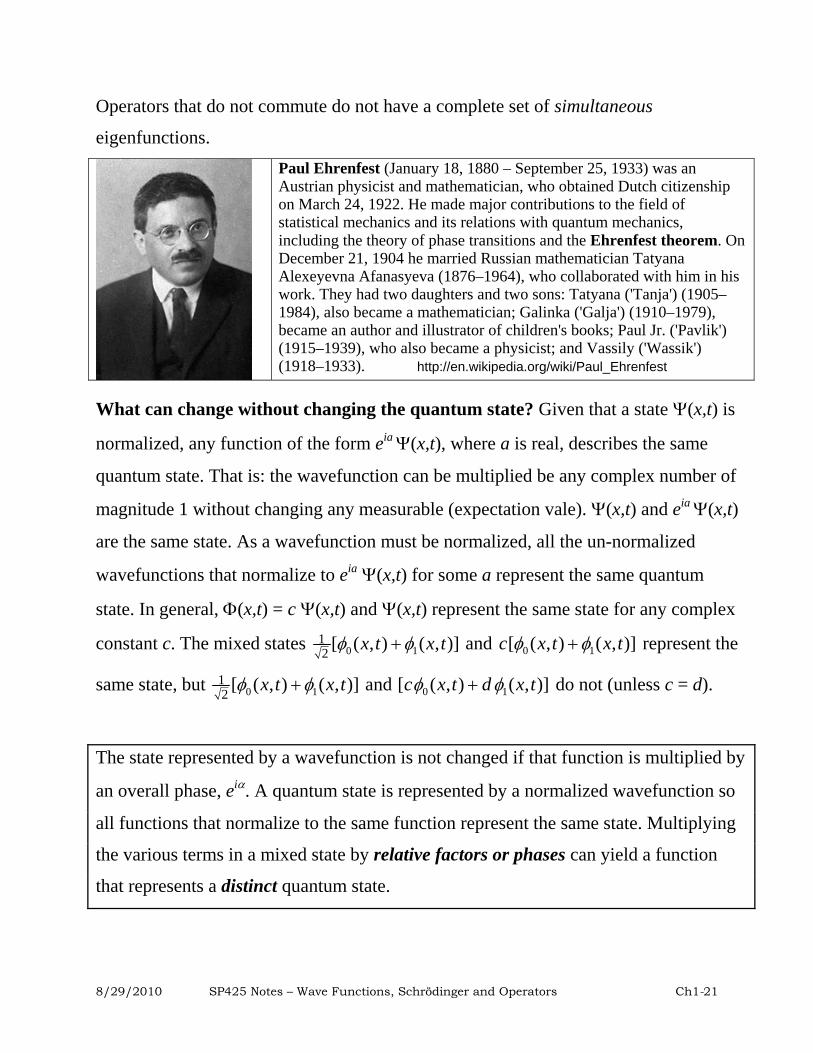
Paul Ehrenfest (January 18, 1880 – September 25, 1933) was an Austrian physicist and mathematician, who obtained Dutch citizenship on March 24, 1922. He made major contributions to the field of statistical mechanics and its relations with quantum mechanics, including the theory of phase transitions and the Ehrenfest theorem. On December 21, 1904 he married Russian mathematician Tatyana Alexeyevna Afanasyeva (1876–1964), who collaborated with him in his work. They had two daughters and two sons: Tatyana ('Tanja') (1905–1984), also became a mathematician; Galinka ('Galja') (1910–1979), became an author and illustrator of children's books; Paul Jr. ('Pavlik') (1915–1939), who also became a physicist; and Vassily ('Wassik') (1918–1933). http://en.wikipedia.org/wiki/Paul_Ehrenfest

What can change without changing the quantum state? Given that a state (x,t) is

normalized, any function of the form eia (x,t), where a is real, describes the same

quantum state. That is: the wavefunction can be multiplied be any complex number of

magnitude 1 without changing any measurable (expectation vale). (x,t) and eia (x,t)

are the same state. As a wavefunction must be normalized, all the un-normalized

wavefunctions that normalize to eia(x,t) for some a represent the same quantum

state. In general, (x,t) = c (x,t) and (x,t) represent the same state for any complex

constant c. The mixed states 0 112

[ ( , ) ( , )]x t x t and 0 1[ ( , ) ( , )]c x t x t represent the

same state, but 0 112

[ ( , ) ( , )]x t x t and [ (0 , )c x t d 1( , )]x t do not (unless c = d).

The state represented by a wavefunction is not changed if that function is multiplied by

an overall phase, ei. A quantum state is represented by a normalized wavefunction so

all functions that normalize to the same function represent the same state. Multiplying

the various terms in a mixed state by relative factors or phases can yield a function

that represents a distinct quantum state.


http://en.wikipedia.org/wiki/Image:Paul_Ehrenfest.jpg�

Wavefunction concavity: For a 1D problem with 2222 ( )m x

V x

as its hamiltonian,

an energy eigenfunction has the form ( , ) ( ) nn n

i tx t u x e where un(x) is a (relatively)

real function (given that V(x) is a real-valued function).

The term relatively real means that the function u(x) is at worst eia, a complex

constant, times a real-valued function. All answers are independent of the overall

phase so we will choose to make the spatial parts of all energy eigenfunctions real.

Each energy eigenfunction obeys the time-independent Schrödinger equation

2 2

2 2

2 2

2 2( ) ( ) ( ) ( ) ( ) ( )n n n nx xm mV x u x E u x u x E V x u x

Regions in which En > V(x) are classically allowed, and regions in which En < V(x) are

classically forbidden. The concavity of the wavefunction 2

2u

x and the wavefunction

u(x) have opposite signs in classically allowed regions, and they have the same sign in

classically forbidden regions. As the spatial wave function is assumed real, these

observations mean that the wavefunctions oscillate back and forth about zero in

allowed regions. The same sign character in forbidden regions corresponds to

behaviors with monotone growth or decay to zero. The decay may have an exponential

character.

A normalizable wavefunction can only exist some region of the domain is classically

allowed. Hence, a solution exists only if E is greater then V(x) for some x.

E must be greater than Vmin in order that a solution exist.

Exercise: Show that the sin(kx) and cos(kx) and their second derivatives have opposite

signs. That is: whenever sin(kx) is positive, its second derivative is negative (it is


concave downward). Make a sketch as a basis to argue that this behavior could cause a

function to oscillate about zero. What is the corresponding result for ex? Sketch a real

function for which the function and its second derivative have the same sign. Can you

generate a consistent sketch in which the function has multiple zeros?

Exercise: Assume that the potential is greater than the energy everywhere so that the

wavefunction and its second derivative have the same sign everywhere. Attempt to

sketch a function with this character in the region - to that you believe could be

normalized. Attempt to sketch a function with this character in the region [a, b] that

would be a continuous function (as required) in the range - to that you believe

could be normalized.

Wavefunction boundary conditions:

The Schrödinger equation (2

2 22( )) [ ( ) ] ( )m

x x V x E x ) involves a second

derivative with respect to the spatial variable. In order that this derivative is defined,

the function and its first derivative must be continuous.

In addition to being normalizable, the behavior requirements for a wave function are:

i.) The wave function must be continuous.

ii.) The first derivative of the wavefunction must be continuous except where V is singular.

We expect the first condition to hold universally. The Schrödinger equation shows

that, the second condition must hold unless the potential is singular (not finite). In fact,

we find that, in one dimension, the second condition holds except at points where the

potential has an infinite discontinuity. The analytic forms of the wavefunction must be

matched to have the same value and slope at any boundary (any point at which the


potential changes its analytic form). For example, the wavefunction value and slope

must be matched at any finite discontinuity of the potential.

Exercise: In one dimension, the second condition holds except at points where the

potential has an infinite discontinuity. Consider the 1S state of a hydrogen atom.

Discuss the situation at r = 0.

At each boundary point, there are free multiplicative constants that allow the ratio of

1(x), the wave function to the left of the boundary and 2(x), the wave function to the

right of the boundary until they are equal. As this operation scales the derivatives by

the same factor, the actual matching conditions are:

2

1 1

2 1

12

( )or

( ) ( ) ( )

d d ddx dx dx

ddx

x

x x

2

x

1 2ln ( ) ln ( )x xx x

The ratio of the derivative of a function to its value is called the logarithmic derivative

of the function. The boundary conditions are summarized in the statement: The limit

of the logarithmic derivative of the wavefunction from the left and from the right

must match at each point at which the potential is finite.

x

V(x)

VO

Region Ix < 0

Region II0<x <a

a0

Region IIIx > a

The Finite Square Well

0

( ) 0

x

ikx ikx

x

Ae x

x C e De x a

F e x a

Match (x) and d/dx at x = 0

and at x = a.


Exercise: Compute the derivative of ln[(x)]. ln natural logarithm

SUMMARY: Properties of the Wavefunction

0.) The wavefunction contains all that can be know about the system.

1.) A wavefunction must satisfy the Schrödinger equation for the problem.

2.) A wavefunction must be normalizable.

3.) A wavefunction must be continuous.

4.) The first spatial derivatives of the wavefunction must be continuous except at

singular points of the potential.

5.) In 1D, the wavefunction is concave toward = 0 in allowed regions and

concave away from = 0 in classically forbidden regions.

Appendix

Basic Review: Lagrangian and Hamiltonian Mechanics:

We restrict our treatment to the simple cases for which the constraints are good, the

potentials are time independent and for which there is no dissipation.

The Lagrangian L is T – V, the kinetic energy minus the potential energy. The

Lagrangian is a natural function of the coordinates qi, the coordinate velocities and

time t. The Lagrange equations of motion are:

iq

i i

d L L

dt q q

The signs and details can be recovered by considering: 2( , , ) ½ ( )L x x t m x V x .

xd L L V

m x Fdt x x x

(recovered Newton’s 2nd Law)


It is crucial to note that the time derivative is a total derivative while the others are

partial derivatives and that x and x are treated as independent variables.

The momentum conjugate to (associated with) a coordinate qi is found as: ii

Lqp .

Using the example: 2( , , ) ½ ( )L x x t m x V x , xp m x . For the planar orbit

problem 2p m r and . 2 2 2 ] (r V ( , , , ) ½ [L r r m r )r

Conservation or constants of the motion:

ii

Lp

q

i i

d L L

dt q q

ii

d Lp

dt q

The momentum pi is a constant of the motion if the Lagrangian does not depend on the

coordinate conjugate to that momentum. Given , there

is no dependence on the angular coordinate so the conjugate momentum

2 2 2( , , , ) ½ [ ] ( )L r r m r r V r

p m2r

is a constant of the motion.

In Hamiltonian mechanics, the coordinates and the momenta are the natural

variables. The hamiltonian is defined to be H = i

i ip q - L. Here pi is the momentum

conjugate to qi as defined based on the lagrangian above. For the simple case: 2( , , ) ½ ( )L x x t m x V x , we find: xp m x .

H(x, px) = 2 2(½ ( )) ½ ( )x xp x m x V x p x m x V x .

We find:

2 2

2( , ) ½ ( ) ( )xxp

mH x p m x V x V x

The hamiltonian is to be expressed as a function of the coordinates and momenta, so

the second form is the one that must be used. For time-independent problems (the type

usually encountered), the hamiltonian represents the total energy of the system.


The Hamilton’s equations of motion are: ii

Hqp

and ii

Hpq

. [WF.19]

Using the example: 2

2( , ) ( )xxp

mH x p V x ,

xi

i

pHq x

p m

and xii

H Vp m x F

q x

Constants of the Motion: The relation ii

Hp

q

shows that pi is a constant of the

motion of the hamiltonian is independent of qi. (Recall that we are restricting our

attention to hamiltonians that do not depend explicitly on time.)

A more general dynamical quantity might have the form and hence have the

total time derivative:

( , , )i iQ q p t

( , , ) ( , , ) ( , , ) ( , , )i i

i i i i i i i i

i i

dQ q p t Q q p t Q q p t Q q p tq pdt q p

t

Using Hamilton’s equations

( , , ) ( , , ) ( , , ) ( , , )

i i

i i i i i i i i

i i

H

p

dQ q p t Q q p t Q q p t Q q p tq pdt

H

q

t

Defining:

( , , ) ( , , )

i i

i i i i

i i

B

p

A q p t A q p tq

B

q

p as [A, B]PB, the Poisson bracket of A and B (where a sum

over the generalized coordinate index i is implicit),

, ][ PBdQ Q

tdt Q H [WF.20]

where: [A, B]PB = ( , , )( , , ) ( , , )( , , )

i i i i

i i

i i i i

i i

B q p t

p

A q p t A q p tq p

B q p t

q

. [WF.21]

Exercise: Show that equation [WF.20] reproduces Hamilton’s equations [WF.19] for

the case that Q is qi and for the case that Q is pi.


Exercise: Show that [qk, p]PB = k where k and are indices labeling the generalized

coordinates. Some of the equations of quantum mechanics can be obtained by setting the quantum commutator equal to i times the corresponding Poisson bracket.

ˆ ˆ[ , ] [ , ]PBA B i A B See [WF.16].

Tools of the Trade

Probability current shortcut:

The probability density is real so we might expect the probability current is real and

measurable. Its form however begins with a factor of i.

Probability current: J(x,t) = *2 *x xim

[WF.22]

If * x is defined to be f(x,t), then the factor in brackets is f * – f = – 2i Im[f].

Hence J(x,t) can be represented as:

J(x,t) = Im * xm

[WF.23]

The Payoff: The result is manifestly real which should set your mind at ease. The true

payoff is that you only need calculate half of the expression in brackets in [WF.22].

Exercise: Compute J(x,t) using equation [WF.23] and the free particle wavefunction

(x,t) = A ei(kx-t).

The Leibnitz rule for the total time derivative of an integral:

2 2

1 1

2 12 1

( , )( , ) ( , ) ( , )x x

x x

dx dxd bb x t dx b x t b x t dxdt dt dt t

x t [WF.24]

For our applications, the limits are fixed so the expression simplifies to:


2 2

1 1

( , )( , )

x x

x x

d bb x t dx dx

dt t

x t

Exercise: Evaluate the equation above for b(x, t) = *(x,t) x (x,t).

Hermitian Property:

Recall the steps in developing the general time dependence of an expectation value.

Identifying and Q H as wavefunctions, and using the Hermitian property:

ˆ ˆ( , ) ( , ) ( , ) ( , )i i i iq t Q q t d Q q t q t d for all and

ˆ ˆˆ ˆ* * *full full fullrange range range

ˆˆH Q dx H Q dx H Q dx

The Hermitian adjoint procedure takes an operator operating in the KET (BRA) and

yields the operator that generates the same result while operating in the BRA (KET).

ˆ ˆO O † or O O † for all and

We used the Hermitian property essentially to declare that:

2 22 2

2 2

*

2 2*full fullrange range

m mx xdx dx

The full hamiltonian and the kinetic energy operator are Hermitian ˆ ˆO O †

Assume the full range is and that and are normalizable wavefunctions.

Use integration by parts to show that: 2 22 2

2 2

**

2 2m mx xdx dx

.

2 22 2 2 2

2 2

* * * *

2 2 2 2m m m m xxx xdx dx dx

x

2

2

2 2* *

2 2m x m xdx

All the surface terms vanish as and vanish at the endpoints.

2

2

22 2

2

**

2 2m m xxdx dx


Thus integration by parts gets the same result as invoking the Hermitian property. For

the case of evaluating dp/dt, the function is essentially x.

322 2

2 3

**

2 2xm mx xdx dx

Conclude that the mysterious Hermitian conjugate operation can be a familiar

operation hiding behind an imposing name.

Appendix: Postulates of Quantum Mechanics

There is no universal agreement on the statements of the postulates of quantum mechanics or

even on the number of postulates. Consider the following to be a starting set. The postulates

must be supplemented and placed in context; they are not sufficient in and of themselves.

Postulate 1:

(The Born Interpretation) There exists a wave function r, t) that completely specifies

the state of a quantum mechanical system. It depends on both the spatial coordinates of

the particle(s) and time, and has the property that r, t) r, t) d denotes the

probability that there is a particle located in a (infinitesimally small) volume d

containing the point at r at time t, where r, t) is the complex conjugate of r, t).

Postulate 2:

The observables in the Hamiltonian formulation of classical mechanics (position,

linear and angular momentum, energy, etc.) are represented quantum mechanically by

Hermitian operators. For each Hermitian operator associated with an observable,

only certain set of values can be measured for that observable; that is the set of

eigenvalues qn that arise from the solution of the eigenvalue equation:

Q

ˆn nQ q n .

The set of all the (eigen-) wavefunctions { … , m, … , .} satisfying this equation can


be chosen to be mutually orthogonal1, and they form a (complete) basis set for all

solutions to the problem. All Hermitian operators have real eigenvalues.

Postulate 3:

The expectation value of an observable represented by at time t in the quantum state

described by r, t) is

Q

* ˆ( , ) ( , )all

r t Q r t d

. The result of any precise measurement

of an observable of a quantum system will be one of the eigenvalues of that

operator, and the result of the measurement will instantaneously collapse the

wavefunction to a state compatible with the outcome of that measurement outcome.

Q

Postulate 4:

Given that the state of the system is expanded in terms of the eigenfunctions n of an

operator Q as app, the probability the a measurement of Q returns the eigenvalue qm

is

2 2| | ( non degenerate)m m m mP a q

( ) 22

1

| | (sum all with q ; if degenerate)n m

m j m j mj

P a j q

It follows that values other than eigenvalues has zero probability of observation.

Postulate 5:

There is a single operator which represents the classical hamiltonian (the energy) of the

system and which is the time-development operator for the wavefunction that describes

the system.

1 Linear combinations of eigenfunction which are degenerate (share the same eigenvalue) can be found that are mutually

orthogonal (Gram-Schmidt).


( , ) ˆ ˆ ˆ( , ) ( , , ) ( , )i jr tti H r t H q p t r t

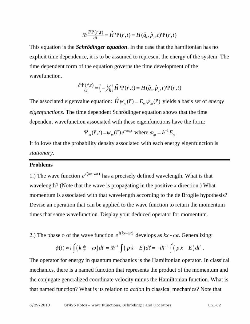
This equation is the Schrödinger equation. In the case that the hamiltonian has no

explicit time dependence, it is to be assumed to represent the energy of the system. The

time dependent form of the equation governs the time development of the

wavefunction.

( , ) ˆ ˆ ˆ( , ) ( , , ) ( , )i jr tt

i H r t H q p t r t

The associated eigenvalue equation: ˆ ( ) ( )m m mH r E r

yields a basis set of energy

eigenfunctions. The time dependent Schrödinger equation shows that the time

dependent wavefunction associated with these eigenfunctions have the form:

1( , ) ( ) wheremi tm m mr t r e E m

It follows that the probability density associated with each energy eigenfunction is

stationary.

Problems

1.) The wave function (i kx te ) has a precisely defined wavelength. What is that

wavelength? (Note that the wave is propagating in the positive x direction.) What

momentum is associated with that wavelength according to the de Broglie hypothesis?

Devise an operation that can be applied to the wave function to return the momentum

times that same wavefunction. Display your deduced operator for momentum.

2.) The phase of the wave function (i kx te ) develops as kx - t. Generalizing:

1 1( )t t t

dxdtt i k dt i p x E dt i p x E dt .

The operator for energy in quantum mechanics is the Hamiltonian operator. In classical

mechanics, there is a named function that represents the product of the momentum and

the conjugate generalized coordinate velocity minus the Hamiltonian function. What is

that named function? What is its relation to action in classical mechanics? Note that


this quantum behavior is the justification for the principle of least (or stationary) action

in classical mechanics.

http://en.wikipedia.org/wiki/Path_integral_formulation or search for Feynman path integral.

3.) Fill in all the steps to reach [WF.7] beginning with [WF.4].

4.) Fill in all the steps required to reach [WF.10] from

* ( , ) ( , )x fullrange

d ddt dtp m x m x t x x t d x

5.) A particle moves in one dimension under the influence of a potential V(x). Its

kinetic energy is . 2½ m x

a.) Give the form of the Lagrangian L(x, x ).

b.) Compute px = Lx , the generalized momentum conjugate to x.

c.) Deduce an expression for the total mechanical energy.

d.) Express that energy as a function of x and px.

e.) Consider the hamiltonian H(x,px) = (1/2m) px2 + V(x). Construct the quantum

operator that represents this Hamiltonian function.

6.) An operator is has the value or is equivalent to its action on an arbitrary function.

Consider the operator [x, px] which is the commutator of x and px.

ˆ ˆ ˆ ˆ ˆ ˆ[ , ]x x x x xx p x p p x i x i x

Let it act on a function f(x). ˆ ˆ[ , ] ( ) ( ) ?x x xx p f x i x i x f x

a.) What is the value of ˆ ˆ[ , ]xx p ? Answer: ˆ ˆ[ , ]xx p i

b.) What is the value of ˆ ˆ[ , ]yx p ? Use g(x,y) as the arbitrary function.


7.) Give the operator for the z component of angular momentum. Lz = x py – y px.

8.) Ignoring spin, the H atom system is described by 1

1 0

( , ) ( , )n

n m n mn m

x t c

x t .

a.) Identify each of the symbols {n, , m}; given the value of each, give the value of

the physical parameter associated with each. b.) A precise energy measurement on a

hydrogen atom returns the energy - 13.6 eV. What is the most general form of the

wavefunction immediately after the measurement? c.) The H atom system is described

by 1

1 0

( , ) ( , )n

n m n mn m

x t c

1

1 0

( , ) ( , )n

n m n mn m

x t . A precise energy measurement on a hydrogen

atom returns the energy - 13.6 eV/4. What is the most general form of the wavefunction

immediately after the measurement? d.) The H atom system is described by

x t c x

t

1

. A precise energy measurement on a hydrogen atom is

followed immediately by a measurement of the square of the electron’s orbital angular

momentum. The measurement pair returns values - 13.6 eV/4 and 2 2. The measurements

are repeated immediately, and the same values are returned. One concludes that

measurements of energy and orbital angular momentum squared are non-interfering.

What is the most general form of the wavefunction immediately after the pair of

measurements? Ignore spin, …

Each of the most general wave functions has one or more undetermined constants.

What constraint does the normalization condition place on these constants in each

case?

9.) The ground state wave function for an electron in a hydrogen atom has the form:

0 1/ ( / ) ( / )100 ( , ) ( )r a i E t i E tr t Ae e u r

. Find the magnitude of the normalization

constant A. Show that the probability density of this pure state is time-independent.


What is the most probable value of r the distance from the nucleus? What are the

expectation values of r, r -1, r2 and r

? (ao is the Bohr radius, 0.0529 nm.)

*** similar to 12 ***

10.) The lowest two states of the QHO have the forms: 2

0 )/20 ( , ) xx t Ae e (½i t and

20

32( )/2

1( , ) i txx t B xe e .

Find real values for the normalization constants A and B. Consider the mixed state

0 112

( , ) [ ( , ) ( , )]x t x t x t . Compute the probability density, x and px for this

mixed state.

11.) Show that the sin(kx) and cos(kx) and their second derivatives have opposite signs.

That is: whenever sin(kx) is positive, its second derivative is negative (it is concave

downward). Make a sketch as a basis to argue that this behavior could cause a function

to oscillate about zero. What is the corresponding result for ex? Use a sketch of a

function for which the function and its second derivative have the same sign. Can you

generate a consistent sketch in which the function has multiple zeros?

12. The ground state wave function for the electron in a hydrogen atom is:

u1S(r,,) = u100(r,,) = 0

30

/1 r aa

e where ao is the Bohr radius 0.0529 nm. The full

wavefunction is (r,,t) = u100(r,,) 1i te , and (r,,t)(r,,t) is

probability density to find the electron in a volume dV = r2 sin d ddr.

a.) Find that the probability density and show that it is time-independent.

b.) Deduce the radial probability density (r) which has the property that is

the probability to find the electron in at a distance between a and b from the nucleus.

( )b

ar dr


c.) Sketch(r,,t)|2 and (r) as functions of r.

d.) Find the most probable value of r.

e.) Compute rthe expectation value of r.

f.) Compute r -1. Give the value of

0

2

4e

r in electron volts.

13. An operator has the value or is equivalent to its action on an arbitrary function.

a.) Consider the operator [x, px] which is the commutator of x and px.

ˆ ˆ ˆ ˆ ˆ ˆ[ , ]x x x x xx p x p p x i x i x

Let it act on a function f(x). ˆ ˆ[ , ] ( ) ( ) ?x x xx p f x i x i x f x

What is the value of ˆ ˆ[ , ]xx p ? Answer: ˆ ˆ[ , ]xx p i

b.) Consider the operator [x, 2

2x ] which is the commutator of x and

2

2x .

Let it act on a function f(x). [x, 2

2x ] f(x) = ?

c.) Consider the operator [x, H ] which is the commutator of x and H where 2

22ˆ ( )m xH V x

. Let it act on a function f(x). [x, H ] f(x) = ?

14.) The commutator ˆ ˆˆ ˆ ˆ[ , ] ˆA B AB B A . a.) Show that ˆ ˆ ˆ ˆ ˆ ˆˆ ˆ ˆ[ , ] [ , ] [ , ]A BC A B C B A C .

Find an analogous relation for ˆ ˆˆ[ , ]AB C . c.) Given that ˆ ˆ[ , ]xx p i , compute . 2ˆ ˆ[ ,( ) ]xx p

15. Compute ˆ[ , ( )] [ , ( )x x ]p g x i g x .

16. Show that the commutators in parts a, b and c vanish: a.) ˆ[ , ] [ ,y y ]p x i x .

b.) [x, y]. c.) ˆ ˆ[ , ]x yp p . d.) Show that ˆ ˆ ˆ ˆ ˆ ˆ[ , ] [ , ]x y z y x zL L y p z p z p x p = ˆzi L .

Reading the statements of the preceding problems is strongly recommended.


17. ˆˆ ˆ[ , ] Qd itdt Q Q H . Applied to the position x, this relation becomes:

ˆ[ , ]d idt x x H . Find d/dtx. Assume

2

22ˆ ( )m xH V x

.

18. ˆˆ ˆ[ , ] Qd itdt Q Q H . Applied to the momentum px, this relation

becomes: ˆ[ ,x xd idt ]p i H

. Find d/dt pxAssume 2

22ˆ ( )m xH V x

.

19. Consider the mixed state 0 112

( , ) [ ( , ) ( , )]x t x t x t where o(x,t) and 1(x,t) are

energy eigenstates with energies o and 1.Show that the probability density is time

dependent. The normalization * ( , ) ( , )x t x t d

x

n

is time independent as long as

. What do we call this condition? 1 0* ( , ) ( , ) 0x t x t dx

20. A Hermitian operator has a complete set of eigenfunctions. Q ˆn nQ q .

a.) Show that the expectation value of in the eigenstate m is qm. Q

b.) Write down the defining condition for the operator to be Hermitian. Q

c.) Show that the eigenvalues of are real. Q

d.) Show that the expectation value of in a mixed state Q1

( , ) ( , )m mm

x t a x t

is

2

1

ˆm m

m

Q a

q .

Conclude that Hermitian operators have real eigenvalues and expectation values. These

properties make them candidates to represent observables.


e.) Show that the expectation value of in a mixed state ˆ( )kQ1

( , ) ( , )m mm

x t a x t

is

2

1

ˆ( ) ( )km m

m

Q a q

k

]

for positive integers k.

21.) Compute the probability currents for a plane wave [i kx tAe , for the mixed

oscillator state and for the mixed box state 2 2[( / ) ] [( / ) 3 ][ a mx it a mx itA e xe ]

42sin( ) ]itx xa[sin( ) it

aA e e for (0 < x < a). Comment on the time dependence of

each result. For the box state case, sketch (x,t)(x,t) for t = 0 and for t = /3.

Evaluate J(½a, t) for the box state case.

Box State Answer: 2 32( , ) [ ] sin[3 ]x

aJ x t A sin tma

Answers are real.

22.) Show that the expectation value of a time-independent operator is a constant in

any state that is an energy eigenfunction of a time-independent Hermitian

hamiltonian. Use 2 2

2ˆ ( )

2H V x

m x

. H E ; E a constant.

ˆˆ ( , ) ( , ) ( , ) ( , ) 0 0i i i i ii

Qq t

d ddt dtQ q p q t Q q i q t d

All expectation values of time-independent operators computed for an energy

eigenstate are time-independent (stationary, dull).

23.) Suppose that the problem:

2 2

2( ) ( , ) ( , ) ( , )

2 n n n nV x x t E x t i x tm x t

[WF.25]

has been solved by separation.


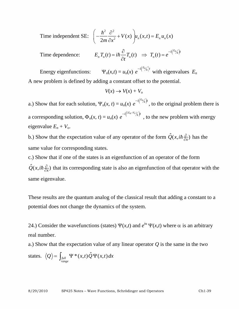
Time independent SE: 2 2

2( ) ( , ) ( )

2 n n nV x u x t E u xm x

Time dependence: ( ) ( )n n nE T t i T tt

( )

En

n

i tT t e

Energy eigenfunctions: n(x,t) = un(x) Enie t

with eigenvalues En

A new problem is defined by adding a constant offset to the potential.

V(x) V(x) + Vo

a.) Show that for each solution, n(x, t) = un(x) Enie t

, to the original problem there is

a corresponding solution, n(x, t) = un(x) 0 ][ E Vni

e t

, to the new problem with energy

eigenvalue En + Vo.

b.) Show that the expectation value of any operator of the form ˆ ( , )xQ x i has the

same value for corresponding states.

c.) Show that if one of the states is an eigenfunction of an operator of the form

ˆ ( , )xQ x i that its corresponding state is also an eigenfunction of that operator with the

same eigenvalue.

These results are the quantum analog of the classical result that adding a constant to a

potential does not change the dynamics of the system.

24.) Consider the wavefunctions (states) (x,t) and ei (x,t) where is an arbitrary

real number.

a.) Show that the expectation value of any linear operator Q is the same in the two

states. ˆ* ( , ) ( , )fullrange

Q x t Q x t dx


b.) Suppose that m(x,t) is an eigenfunction for Q with eigenvalue qm. Show that

ei m(x,t) is also an eigenfunction for Q with eigenvalue qm.

c.) Consider m(x,t) and c m(x,t) where c is an arbitrary complex number. Suppose

that m(x,t) is an eigenfunction for Q with eigenvalue qm. Show that c m(x,t) is also an

eigenfunction for Q with eigenvalue qm. Show that every expectation value computed

for m(x,t) and c m(x,t) are identical provided the calculations include a normalizing

denominator.

ˆ* ( , ) ( , )

* ( , ) ( , )

fullrange

fullrange

x t Q x t dxQ

x t x t dx

25.) Consider the wavefunctions 0 112

[ ( , ) ( , )]x t x t and 0 1[ ( , ) ( , )c x t d x t ] . The

two functions o(x,t) and 1(x,t) are eigenfunctions of energy with distinct eigenvalues

o and 1. Show that 0 1[ ( , ) ( , )c x t d x t ] is not an eigenfunction of energy unless c or

d equals zero. Compute the expectation value of the hamiltonian for the states

0 112

[ ( , ) ( , )]x t x t ] and 0[ ( , )c x t d 1( , )x t . Does the expectation value of the

energy of the state depend on time?

26.) The Leibnitz rule for the total time derivative of an integral:

2 2

1 1

2 12 1

( , )( , ) ( , ) ( , )

x x

x x

dx dxd bb x t dx b x t b x t dx

dt dt dt t

x t [WF.26]

For our applications, the limits are fixed so the expression simplifies to:

2 2

1 1

( , )( , )

x x

x x

d bb x t dx dx

dt t

x t

a.) Evaluate this result for b(x,t) = *(x,t) x (x,t).

b.) Consider ( )

( )( , )

b t

a t

d

dtb x t dx

. Show that:


( ) ( ) ( )

( ) ( ) ( )

2

( , ) ( , ) [ ( , ) ( , )]

( ( ))[ ( ) ( )] ( ( ))[ ( ) ( )]

[ ]

b t t b t b t

a t t a t a tf x t t dx f x t dx f x t t f x t dx

f b t b t t b t f a t a t t a t

Terms of Order t

Use this to justify the form of the Leibnitz relation.

We motivated the identification of the momentum operator by considering:

*( , ) ( , )* ( , ) ( , ) ( , ) * ( , )full fullrange range

x t x td dt tdt dtx x t x x t dx x x t x t x dx

The development employed calculus, Schrödinger’s equation and lengthy equations to

overwhelm the student into accepting the identification: ˆ x xp i . Now I claim that

the argument could be considered to be circular. Review the argument. Explain why it

might be considered to be circular.

References:

1. David J. Griffiths, Introduction to Quantum Mechanics, 2nd

Edition, Pearson Prentice Hall (2005).

2. Richard Fitzpatrick, Quantum Mechanics Note Set, University of Texas.


1. the wave function, s.e. and basic operators · 2010. 8. 29. · operators, expectation values...

Documents