1

Towards Bayesian Deep Learning:A Survey

Hao Wang, Dit-Yan YeungHong Kong University of Science and Technology

hwangaz,dyyeung@cse.ust.hk

Abstract—While perception tasks such as visual object recognition and text understanding play an important role in humanintelligence, the subsequent tasks that involve inference, reasoning and planning require an even higher level of intelligence. The pastfew years have seen major advances in many perception tasks using deep learning models. For higher-level inference, however,probabilistic graphical models with their Bayesian nature are still more powerful and flexible. To achieve integrated intelligence thatinvolves both perception and inference, it is naturally desirable to tightly integrate deep learning and Bayesian models within aprincipled probabilistic framework, which we call Bayesian deep learning. In this unified framework, the perception of text or imagesusing deep learning can boost the performance of higher-level inference and in return, the feedback from the inference process is ableto enhance the perception of text or images. This survey provides a general introduction to Bayesian deep learning and reviews itsrecent applications on recommender systems, topic models, and control. In this survey, we also discuss the relationship anddifferences between Bayesian deep learning and other related topics like Bayesian treatment of neural networks.

Index Terms—Bayesian Networks, Neural Networks, Deep Learning, Data Mining, Machine Learning, Artificial Intelligence

F

1 INTRODUCTION

D EEP learning has achieved significant success inmany perception tasks including seeing (visual object

recognition), reading (text understanding), and hearing(speech recognition). These are undoubtedly fundamentaltasks for a functioning comprehensive artificial intelligence(AI) system. However, in order to build a real AI system,simply being able to see, read, and hear is far from enough.It should, above all, possess the ability of thinking.

Take medical diagnosis as an example. Besides seeingvisible symptoms (or medical images from CT) and hearingdescriptions from patients, a doctor has to look for relationsamong all the symptoms and preferably infer the etiology ofthem. Only after that can the doctor provide medical advicefor the patients. In this example, although the abilities ofseeing and hearing allow the doctor to acquire informationfrom the patients, it is the thinking part that defines a doctor.Specifically, the ability of thinking here could involve causalinference, logic deduction, and dealing with uncertainty,which is apparently beyond the capability of conventionaldeep learning methods. Fortunately, another type of models,probabilistic graphical models (PGM), excels at causalinference and dealing with uncertainty. The problem is thatPGM is not as good as deep learning models at perceptiontasks. To address the problem, it is, therefore, a naturalchoice to tightly integrate deep learning and PGM within aprincipled probabilistic framework, which we call Bayesiandeep learning (BDL) in this paper.

With the tight and principled integration in Bayesiandeep learning, the perception task and inference task areregarded as a whole and can benefit from each other. Inthe example above, being able to see the medical imagecould help with the doctor’s diagnosis and inference. Onthe other hand, diagnosis and inference can in return helpwith understanding the medical image. Suppose the doctor

may not be sure about what a dark spot in a medical imageis, but if she is able to infer the etiology of the symptoms anddisease, it can help him better decide whether the dark spotis a tumor or not.

As another example, to achieve high accuracy inrecommender systems [45], [60], we need to fullyunderstand the content of items (e.g., documents andmovies), analyze the profile and preference of users, andevaluate the similarity among users. Deep learning is goodat the first subtask while PGM excels at the other two.Besides the fact that better understanding of item contentwould help with the analysis of user profiles, the estimatedsimilarity among users could provide valuable informationfor understanding item content in return. In order to fullyutilize this bidirectional effect to boost recommendationaccuracy, we might wish to unify deep learning and PGMin one single principled probabilistic framework, as done in[60].

Besides recommender systems, the need for Bayesiandeep learning may also arise when we are dealing withcontrol of non-linear dynamical systems with raw imagesas input. Consider controlling a complex dynamical systemaccording to the live video stream received from a camera.This problem can be transformed into iteratively performingtwo tasks, perception from raw images and control basedon dynamic models. The perception task can be taken careof using multiple layers of simple nonlinear transformation(deep learning) while the control task usually needsmore sophisticated models like hidden Markov modelsand Kalman filters [21], [38]. The feedback loop is thencompleted by the fact that actions chosen by the controlmodel can affect the received video stream in return. Toenable an effective iterative process between the perceptiontask and the control task, we need two-way information

arX

iv:1

604.

0166

2v2

[st

at.M

L]

7 A

pr 2

016

2

exchange between them. The perception component wouldbe the basis on which the control component estimates itsstates and the control component with a dynamic modelbuilt in would be able to predict the future trajectory(images). In such cases, Bayesian deep learning is a suitablechoice [62].

Apart from the major advantage that BDL provides aprincipled way of unifying deep learning and PGM, anotherbenefit comes from the implicit regularization built in BDL.By imposing a prior on hidden units, parameters defininga neural network, or the model parameters specifyingthe causal inference, BDL can to some degree avoidoverfitting, especially when we do not have sufficientdata. Usually, a BDL model consists of two components,a perception component that is a Bayesian formulationof a certain type of neural networks and a task-specificcomponent that describes the relationship among differenthidden or observed variables using PGM. Regularization iscrucial for them both. Neural networks usually have largenumbers of free parameters that need to be regularizedproperly. Regularization techniques like weight decay anddropout [51] are shown to be effective in improvingperformance of neural networks and they both haveBayesian interpretations [13]. In terms of the task-specificcomponent, expert knowledge or prior information, as akind of regularization, can be incorporated into the modelthrough the prior we imposed to guide the model when dataare scarce.

Yet another advantage of using BDL for complex tasks(tasks that need both perception and inference) is thatit provides a principled Bayesian approach of handlingparameter uncertainty. When BDL is applied to complextasks, there are three kinds of parameter uncertainty that needto be taken into account:

1) Uncertainty on the neural network parameters.2) Uncertainty on the task-specific parameters.3) Uncertainty of exchanging information between the

perception component and the task-specific component.By representing the unknown parameters usingdistributions instead of point estimates, BDL offers apromising framework to handle these three kinds ofuncertainty in a unified way. It is worth noting that thethird uncertainty could only be handled under a unifiedframework like BDL. If we train the perception componentand the task-specific component separately, it is equivalentto assuming no uncertainty when exchanging informationbetween the two components.

Of course, there are challenges when applying BDLto real-world tasks. (1) First, it is nontrivial to designan efficient Bayesian formulation of neural networks withreasonable time complexity. This line of work is pioneeredby [24], [37], [40], but it has not been widely adopted dueto its lack of scalability. Fortunately, some recent advancesin this direction [1], [7], [19], [22], [32] seem to shed lighton the practical adoption of Bayesian neural network1. (2)The second challenge is to ensure efficient and effectiveinformation exchange between the perception component

1. Here we refer to Bayesian treatment of neural networks asBayesian neural network. The other term, Bayesian deep learning, isretained to refer to complex Bayesian models with both a perceptioncomponent and a task-specific component.

and the task-specific component. Ideally both the first-orderand second-order information (e.g., the mean and thevariance) should be able to flow back and forth betweenthe two components. A natural way is to represent theperception component as a PGM and seamlessly connectit to the task-specific PGM, as done in [15], [59], [60].

In this survey, we aim to give a comprehensive overviewof BDL models for recommender systems, topic models (andrepresentation learning), and control. The rest of the surveyis organized as follows: In Section 2, we provide a reviewof some basic deep learning models. Section 3 covers themain concepts and techniques for PGM. These two sectionsserve as the background for BDL, and the next section,Section 4, would survey the BDL models applied to areaslike recommender systems and control. Section 5 discussessome future research issues and concludes the paper.

2 DEEP LEARNING

Deep learning normally refers to neural networks withmore than two layers. To better understand deep learning,here we start with the simplest type of neural networks,multilayer perceptrons (MLP), as an example to showhow conventional deep learning works. After that, we willreview several other types of deep learning models basedon MLP.

2.1 Multilayer Perceptron

Essentially a multilayer perceptron is a sequence ofparametric nonlinear transformations. Suppose we want totrain a multilayer perceptron to perform a regression taskwhich maps a vector of M dimensions to a vector of Ddimensions. We denote the input as a matrix X0 (0 meansit is the 0-th layer of the perceptron). The j-th row of X0,denoted as X0,j∗, is an M -dimensional vector representingone data point. The target (the output we want to fit)is denoted as Y. Similarly Yj∗ denotes a D-dimensionalrow vector. The problem of learning an L-layer multilayerperceptron can be formulated as the following optimizationproblem:

minWl,bl

‖XL −Y‖F + λ∑l

‖Wl‖2F

subject to Xl = σ(Xl−1Wl + bl), l = 1, . . . , L− 1

XL = XL−1WL + bL,

where σ(·) is an element-wise sigmoid function for amatrix and σ(x) = 1

1+exp(−x) . The purpose of imposingσ(·) is to allow nonlinear transformation. Normally othertransformations like tanh(x) and max(0, x) can be used asalternatives of the sigmoid function.

Here Xl (l = 1, 2, . . . , L − 1) is the hidden units. Aswe can see, XL can be easily computed once X0, Wl,and bl are given. Since X0 is given by the data, we onlyneed to learn Wl and bl here. Usually this is done usingbackpropagation and stochastic gradient descent (SGD). Thekey is to compute the gradients of the objective functionwith respect to Wl and bl. If we denote the value of the

3

X0X0 X1X1 X2X2 X3X3 X4X4 XcXc

Fig. 1. A 2-layer SDAE with L = 4.

objective function as E, we can compute the gradients usingthe chain rule as:

∂E

∂XL= 2(XL −Y) (1)

∂E

∂Xl= (

∂E

∂Xl+1Xl+1 (1−Xl+1))Wl+1 (2)

∂E

∂Wl= XT

l−1(∂E

∂XlXl (1−Xl)) (3)

∂E

∂bl= mean(

∂E

∂XlXl (1−Xl), 1), (4)

where l = 1, . . . , L and the regularization terms are omitted. denotes the element-wise product and mean(·, 1) is thematlab operation on matrices. In practice, we only use asmall part of the data (e.g., 128 data points) to compute thegradients for each update. This is called stochastic gradientdescent.

As we can see, in conventional deep learning models,only Wl and bl are free parameters, which we will updatein each iteration of the optimization. Xl is not a freeparameter since it can be computed exactly if Wl and blare given.

2.2 Autoencoders

An autoencoder (AE) is a feedforward neural networkto encode the input into a more compact representationand reconstruct the input with the learned representation.In its simplest form, an autoencoder is no more than amultilayer perceptron with a bottleneck layer (a layer witha small number of hidden units) in the middle. The idea ofautoencoders has been around for decades [8], [18], [25], [33]and abundant variants of autoencoders have been proposedto enhance representation learning including sparse AE [43],contrastive AE [46], and denoising AE [54]. For more details,please refer to a nice recent book on deep learning [18]. Herewe introduce a kind of multilayer denoising AE, known asstacked denoising autoencoders (SDAE), both as an exampleof AE variants and as background for its applications onBDL-based recommender systems in Section 4.

SDAE [54] is a feedforward neural network for learningrepresentations (encoding) of the input data by learningto predict the clean input itself in the output, as shownin Figure 1. The hidden layer in the middle, i.e., X2 inthe figure, can be constrained to be a bottleneck to learncompact representations. The difference between traditionalAE and SDAE is that the input layer X0 is a corruptedversion of the clean input data. Essentially an SDAE solves

Fig. 2. A convolutional layer with 4 input feature maps and 2 outputfeature maps.

the following optimization problem:

minWl,bl

‖Xc −XL‖2F + λ∑l

‖Wl‖2F

subject to Xl = σ(Xl−1Wl + bl), l = 1, . . . , L− 1

XL = XL−1WL + bL,

where λ is a regularization parameter and ‖ · ‖F denotes theFrobenius norm. Here SDAE can be regarded as a multilayerperceptron for regression tasks described in the previoussection. The input X0 of the MLP is the corrupted versionof the data and the target Y is the clean version of the dataXc. For example, Xc can be the raw data matrix, and we canrandomly set 30% of the entries in Xc to 0 and get X0. In anutshell, SDAE learns a neural network that takes the noisydata as input and recovers the clean data in the last layer.This is what ‘denoising’ in the name means. Normally, theoutput of the middle layer, i.e., X2 in Figure 1, would beused to compactly represent the data.

2.3 Convolutional Neural NetworksConvolutional neural networks (CNN) can be viewed asanother variant of MLP. Different from AE, which is initiallydesigned to perform dimensionality reduction, CNN isbiologically inspired. According to [29], two types of cellshave been identified in the cat’s visual cortex. One is simplecells that respond maximally to specific patterns withintheir receptive field, and the other is complex cells withlarger receptive field that are considered locally invariantto positions of patterns. Inspired by these findings, the twokey concepts in CNN are then developed: convolution andmax-pooling.

Convolution: In CNN, a feature map is the result of theconvolution of the input and a linear filter, followed by someelement-wise nonlinear transformation. The input here canbe the raw image or the feature map from the previous layer.Specifically, with input X, weights Wk, bias bk, the k-thfeature map Hk can be obtained as follows:

Hkij = tanh((Wk ∗X)ij + bk).

Note that in the equation above we assume one single inputfeature map and multiple output feature maps. In practice,CNN often has multiple input feature maps as well due toits deep structure. A convolutional layer with 4 input featuremaps and 2 output feature maps is shown in Figure 2.

Max-Pooling: Usually, a convolutional layer in CNNis followed by a max-pooling layer, which can be seenas a type of nonlinear downsampling. The operation ofmax-pooling is simple. For example, if we have a featuremap of size 6 × 9, the result of max-pooling with a 3 × 3region would be a downsampled feature map of size

4

xxWW

zzVV

oo

xtxt

htht

otot

WW

Fig. 3. On the left is a conventional feedforward neural network with onehidden layer, where x is the input, z is the hidden layer, and o is theoutput, W and V are the corresponding weights (biases are omittedhere). On the right is a recurrent neural network with input xtTt=1,hidden states htTt=1, and output otTt=1.

x1x1

h1h1

o1o1

YY

VV

x2x2

h2h2

o2o2

YY

VV. . .. . .

xTxT

hThT

oToT

YY

VVWW WW

Fig. 4. An unrolled RNN which is equivalent to the one in Figure 3(right).Here each node (e.g., x1, h1, or o1) is associated with one particulartime instance.

2 × 3. Each entry of the downsampled feature map is themaximum value of the corresponding 3 × 3 region in the6 × 9 feature map. Max-pooling layers can not only reducecomputational cost by ignoring the non-maximal entries butalso provide local translation invariance.

Putting it all together: Usually to form a completeand working CNN, the input would alternate betweenL convolutional layers and L max-pooling layers beforegoing into an MLP for tasks like classification or regression.One famous example is the LeNet-5 [34], which alternatesbetween 2 convolutional layers and 2 max-pooling layersbefore going into a fully connected MLP for target tasks.

2.4 Recurrent Neural Network

When we read an article, we would normally take inone word at a time and try to understand the currentword based on previous words. This is a recurrent processthat needs short-term memory. Unfortunately conventionalfeedforward neural networks like the one shown in Figure3(left) fail to do so. For example, imagine we want toconstantly predict the next word as we read an article.Since the feedforward network only computes the output oas Vq(Wx), where the function q(·) denotes element-wisenonlinear transformation, it is unclear how the networkcould naturally model the sequence of words to predict thenext word.

2.4.1 Vanilla Recurrent Neural Network

To solve the problem, we need a recurrent neuralnetwork [18] instead of a feedforward one. As shown inFigure 3(right), the computation of the current hidden statesht depends on the current input xt (e.g., the t-th word) andthe previous hidden states ht−1. This is why there is a loopin the RNN. It is this loop that enables short-term memoryin RNNs. The ht in the RNN represents what the networkknows so far at the t-th time step. To see the computationmore clearly, we can unroll the loop and represent the RNN

as in Figure 4. If we use hyperbolic tangent nonlinearity(tanh), the computation of output ot will be as follows:

at = Wht−1 + Yxt + b

ht = tanh(at)

ot = Vht + c,

where Y, W, and V denote the weight matrices forinput-to-hidden, hidden-to-hidden, and hidden-to-outputconnections, respectively, and b and c are the correspondingbiases. If the task is to classify the input data at eachtime step, we can compute the classification probability aspt = softmax(ot) where

softmax(q) =exp(q)∑iexp(qi)

.

Similar to feedforward networks, to train an RNN,a generalized back-propagation algorithm calledback-propagation through time (BPTT) [18] can be used.Essentially the gradients are computed through theunrolled network as shown in Figure 4 with shared weightsand biases for all time steps.

2.4.2 Gated Recurrent Neural NetworkThe problem with the vanilla RNN introduced above isthat the gradients propagated over many time steps areprone to vanish or explode, which makes the optimizationnotoriously difficult. In addition, the signal passing throughthe RNN decays exponentially, making it impossible tomodel long-term dependencies in long sequences. Imaginewe want to predict the last word in the paragraph ‘I havemany books ... I like reading’. In order to get the answer, weneed ‘long-term memory’ to retrieve information (the word‘books’) at the start of the text. To address this problem,the long short-term memory model (LSTM) is designed asa type of gated RNN to model and accumulate informationover a relatively long duration. The intuition behind LSTMis that when processing a sequence consisting of severalsubsequences, it is sometimes useful for the neural networkto summarize or forget the old states before moving onto process the next subsequence [18]. Using t = 1 . . . Tjto index the words in the sequence, the formulation ofLSTM is as follows (we drop the item index j for notationalsimplicity):

xt = Wwet

st = hft−1 st−1 + hit−1 σ(Yxt−1 + Wht−1 + b), (5)

where xt is the word embedding of the t-th word, Ww isa KW -by-S word embedding matrix, and et is the 1-of-Srepresentation, stands for the element-wise productoperation between two vectors, σ(·) denotes the sigmoidfunction, st is the cell state of the t-th word, and b, Y,and W denote the biases, input weights, and recurrentweights respectively. The forget gate units hft and the inputgate units hit in Equation (5) can be computed using theircorresponding weights and biases Yf , Wf , Yi, Wi, bf ,and bi:

hft = σ(Yfxt + Wfht + bf )

hit = σ(Yixt + Wiht + bi).

5

A B C $ A B C $

Fig. 5. The encoder-decoder architecture involving two LSTMs. The encoder LSTM (in the left rectangle) encodes the sequence ‘ABC’ into arepresentation and the decoder LSTM (in the right rectangle) recovers the sequence from the representation. ‘$’ marks the end of a sentence.

k

KJ

z wD

Fig. 6. The probabilistic graphical model for LDA, J is the number of documents and D is the number of words in a document.

The output depends on the output gate hot which has itsown weights and biases Yo, Wo, and bo:

ht = tanh(st) hot−1hot = σ(Yoxt + Woht + bo).

Note that in the LSTM, information of the processedsequence is contained in the cell states st and the outputstates ht, both of which are column vectors of length KW .

Similar to [12], [53], we can use the output state and cellstate at the last time step (hTj and sTj ) of the first LSTM asthe initial output state and cell state of the second LSTM.This way the two LSTMs can be concatenated to form anencoder-decoder architecture, as shown in Figure 5.

Note that there is a vast literature on deep learning andneural networks. The introduction in this section intends toserve only as the background of Bayesian deep learning.Readers are referred to [18] for a comprehensive survey andmore details.

3 PROBABILISTIC GRAPHICAL MODELS

Probabilistic Graphical Models (PGM) use diagrammaticrepresentations to describe random variables andrelationships among them. Similar to a graph thatcontains nodes (vertices) and links (edges), PGM hasnodes to represent random variables and links to expressprobabilistic relationships among them.

3.1 ModelsThere are essentially two types of PGM, directed PGM (alsoknown as Bayesian networks) and undirected PGM (alsoknown as Markov random fields). In this survey we mainlyfocus on directed PGM2. For details on undirected PGM,readers are referred to [3].

A classic example of PGM would be latent Dirichletallocation (LDA), which is used as a topic model to analyzethe generation of words and topics in documents. UsuallyPGM comes with a graphical representation of the modeland a generative process to depict the story of how therandom variables are generated step by step. Figure 6shows the graphical model for LDA and the correspondinggenerative process is as follows:• For each document j (j = 1, 2, . . . , J ),

1) Draw topic proportions θj ∼ Dirichlet(α).2) For each word wjn of item (paper) wj ,

2. For convenience, PGM stands for directed PGM in this surveyunless specified otherwise.

a) Draw topic assignment zjn ∼ Mult(θj).b) Draw word wjn ∼ Mult(βzjn).

The generative process above gives the story of how therandom variables are generated. In the graphical model inFigure 6, the shaded node denotes observed variables whilethe others are latent variables (θ and z) or parameters (αand β). As we can see, once the model is defined, learningalgorithms can be applied to automatically learn the latentvariables and parameters.

Due to its Bayesian nature, PGM like LDA is easyto extend to incorporate other information or to performother tasks. For example, after LDA, different variants oftopic models based on it have been proposed. [5], [56]are proposed to incorporate temporal information and[4] extends LDA by assuming correlations among topics.[26] extends LDA from the batch mode to the onlinesetting, making it possible to process large datasets. Onrecommender systems, [55] extends LDA to incorporaterating information and make recommendations. This modelis then further extended to incorporate social information[44], [57], [58].

3.2 Inference and Learning

Strictly speaking, the process of finding the parameters (e.g.,α and β in Figure 6) is called learning and the processof finding the latent variables (e.g., θ and z in Figure 6)given the parameters is called inference. However, givenonly the observed variables (e.g. w in Figure 6), learningand inference are often intertwined. Usually the learningand inference of LDA would alternate between the updatesof latent variables (which correspond to inference) and theupdates of the parameters (which correspond to learning).Once the learning and inference of LDA is completed, wewould have the parameters α and β. If a new documentcomes, we can now fix the learned α and β and then performinference alone to find the topic proportions θj of the newdocument.3

Like in LDA, various learning and inference algorithmsare available for each PGM. Among them, the mostcost-effective one is probably maximum a posteriori (MAP),which amounts to maximizing the posterior probabilityof the latent variable. Using MAP, the learning processis equivalent to minimizing (or maximizing) an objectivefunction with regularization. One famous example is theprobabilistic matrix factorization (PMF) [48]. The learning

3. For convenience, we use ‘learning’ to represent both ‘learning andinference’ in the following text.

6

TABLE 1Summary of BDL Models

Applications Models Ωh Variance of Ωh MAP VI Gibbs Sampling SG Thermostats

RecommenderSystems

CDL V Hyper-Variance XBayesian CDL V Hyper-Variance XMarginalized CDL V Learnable Variance XSymmetric CDL V,U Learnable Variance XCollaborative Deep Ranking V Hyper-Variance X

TopicModels

Relational SDAE S Hyper-Variance XDPFA-SBN X Zero-Variance X XDPFA-RBM X Zero-Variance X X

Control Embed to Control zt, zt+1 Learnable Variance X

of the graphical model in PMF is equivalent to factorizationof a large matrix into two low-rank matrices with L2regularization.

MAP, as efficient as it is, gives us only point estimatesof latent variables (and parameters). In order to take theuncertainty into account and harness the full power ofBayesian models, one would have to resort to Bayesiantreatments like variational inference and Markov chainMonte Carlo (MCMC). For example, the original LDAuses variational inference to approximate the true posteriorwith factorized variational distributions [6]. Learning ofthe latent variables and parameters then boils down tominimizing the KL-divergence between the variationaldistributions and the true posterior distributions. Besidesvariational inference, another choice for a Bayesiantreatment is to use MCMC. For example, MCMC algorithmslike [42] have been proposed to learn the posteriordistributions of LDA.

4 BAYESIAN DEEP LEARNING

With the background on deep learning and PGM, weare now ready to introduce the general framework andsome concrete examples of BDL. Specifically, in this sectionwe will list some recent BDL models with applicationson recommender systems, topic models, and control. Asummary of these models is shown in Table 1.

4.1 General Framework

As mentioned in Section 1, BDL is a principled probabilisticframework with two seamlessly integrated components: aperception component and a task-specific component.

PGM for BDL: Figure 7 shows the PGM of a simple BDLmodel as an example. The part inside the red rectangle onthe left represents the perception component and the partinside the blue rectangle on the right is the task-specificcomponent. Typically, the perception component wouldbe a probabilistic formulation of a deep learning modelwith multiple nonlinear processing layers represented asa chain structure in the PGM. While the nodes and edgesin the perception component are relatively simple, those inthe task-specific component often describe more complexdistributions and relationships among variables (like inLDA).

Three Sets of Variables: There are three sets of variablesin a BDL model: perception variables, hinge variables, andtask variables. In this paper, we use Ωp to denote the set ofperception variables (e.g., A, B, and C in Figure 7), whichare the variables in the perception component. Usually Ωp

would include the weights and neurons in the probabilistic

AA BB CC

DD EE FF

JJ GG

II HH

Fig. 7. The PGM for an example BDL. The red rectangle on the leftindicates the perception component, and the blue rectangle on the rightindicates the task-specific component. The hinge variable Ω = J.

formulation of a deep learning model. Ωh is used to denotethe set of hinge variables (e.g. J in Figure 7). These variablesdirectly interact with the perception component from thetask-specific component. Table 1 shows the set of hingevariables Ωh for each listed BDL models. The set of taskvariables (e.g. G, I, and H in Figure 7), i.e., variables inthe task-specific component without direct relation to theperception component, is denoted as Ωt.

The I.I.D. Requirement: Note that hinge variablesare always in the task-specific component. Normally, theconnections between hinge variables Ωh and the perceptioncomponent (e.g., C → J and F → J in Figure 7) shouldbe i.i.d. for convenience of parallel computation in theperception component. For example, each row in J isrelated to only one corresponding row in C and one in F.Although it is not mandatory in BDL models, meeting thisrequirement would significantly increase the efficiency ofparallel computation in model training.

Joint Distribution Decomposition: If the edges betweenthe two components point towards Ωh, the joint distributionof all variables can be written as:

p(Ωp,Ωh,Ωt) = p(Ωp)p(Ωh|Ωp)p(Ωt|Ωh). (6)

If the edges between the two components originate fromΩh, the joint distribution of all variables can be written as:

p(Ωp,Ωh,Ωt) = p(Ωt)p(Ωh|Ωt)p(Ωp|Ωh). (7)

Apparently, it is possible for BDL to have some edgesbetween the two components pointing towards Ωh andsome originating from Ωh, in which case the decompositionof the joint distribution would be more complex.

Variance Related to Ωh: As mentioned in Section 1, oneof the motivations for BDL is to model the uncertainty ofexchanging information between the perception componentand the task-specific component, which boils down tomodeling the uncertainty related to Ωh. For example, thiskind of uncertainty is reflected in the variance of theconditional density p(Ωh|Ωp) in Equation (6)4. Accordingto the degree of flexibility, there are three types of variance

4. For models with the joint likelihood decomposed as in Equation(7), the uncertainty is reflected in the variance of p(Ωp|Ωh).

7

for Ωh (for simplicity we assume the joint likelihood of BDLis Equation (6), Ωp = p, Ωh = h, and p(Ωh|Ωp) =N (h|p, s) in our example):• Zero-Variance: Zero-Variance (ZV) assumes no

uncertainty during the information exchange betweenthe two components. In the example, zero-variancemeans directly setting s to 0.

• Hyper-Variance: Hyper-Variance (HV) assumes thatuncertainty during the information exchange is definedthrough hyperparameters. In the example, HV meansthat s is a hyperparameter that is manually tuned.

• Learnable Variance: Learnable Variance (LV) useslearnable parameters to represent uncertainty duringthe information exchange. In the example, s is thelearnable parameter.

As shown above, we can see that in terms of modelflexibility, LV > HV > ZV. Normally, if the models areproperly regularized, an LV model would outperform anHV model, which is superior to a ZV model. In Table 1,we show the types of variance for Ωh in different BDLmodels. Note that although each model in the table has aspecific type, one can always adjust the models to devisetheir counterparts of other types. For example, while CDLin the table is an HV model, we can easily adjust p(Ωh|Ωp)in CDL to devise its ZV and LV counterparts. In [60],they compare the performance of an HV CDL and a ZVCDL and finds that the former performs significantly better,meaning that sophisticatedly modeling uncertainty betweentwo components is essential for performance.

Learning Algorithms: Due to the nature of BDL,practical learning algorithms need to meet these criteria:

1) They should be online algorithms in order to scale wellfor large datasets.

2) They should be efficient enough to scale linearlywith the number of free parameters in the perceptioncomponent.

Criterion (1) implies that conventional variational inferenceor MCMC methods are not applicable. Usually an onlineversion of them is needed [27]. Most SGD-based methodsdo not work either unless only MAP inference (as opposedto Bayesian treatments) is performed. Criterion (2) isneeded because there are typically a large number offree parameters in the perception component. This meansmethods based on Laplace approximation [37] are notrealistic since they involve the computation of a Hessianmatrix that scales quadratically with the number of freeparameters.

4.2 Bayesian Deep Learning for RecommenderSystems

Despite the successful applications of deep learningon natural language processing and computer vision,very few attempts have been made to develop deeplearning models for CF. [49] uses restricted Boltzmannmachines instead of the conventional matrix factorizationformulation to perform CF and [17] extends this workby incorporating user-user and item-item correlations.Although these methods involve both deep learning andCF, they actually belong to CF-based methods becausethey do not incorporate content information like CTR

[55], which is crucial for accurate recommendation. [47]uses low-rank matrix factorization in the last weightlayer of a deep network to significantly reduce thenumber of model parameters and speed up training,but it is for classification instead of recommendationtasks. On music recommendation, [41], [61] directly useconventional CNN or deep belief networks (DBN) to assistrepresentation learning for content information, but thedeep learning components of their models are deterministicwithout modeling the noise and hence they are lessrobust. The models achieve performance boost mainly byloosely coupled methods without exploiting the interactionbetween content information and ratings. Besides, the CNNis linked directly to the rating matrix, which means themodels will perform poorly due to serious overfitting whenthe ratings are sparse.

4.2.1 Collaborative Deep LearningTo address the challenges above, a hierarchical Bayesianmodel called collaborative deep learning (CDL) as a noveltightly coupled method for RS is introduced in [60]. Basedon a Bayesian formulation of SDAE, CDL tightly couplesdeep representation learning for the content informationand collaborative filtering for the rating (feedback) matrix,allowing two-way interaction between the two. Experimentsshow that CDL significantly outperforms the state of the art.

In the following text, we will start with the introductionof the notation used during our presentation of CDL. Afterthat we will review the design and learning of CDL.

Notation and Problem Formulation: Similar to the workin [55], the recommendation task considered in CDL takesimplicit feedback [28] as the training and test data. Theentire collection of J items (articles or movies) is representedby a J -by-B matrix Xc, where row j is the bag-of-wordsvector Xc,j∗ for item j based on a vocabulary of size B.With I users, we define an I-by-J binary rating matrixR = [Rij ]I×J . For example, in the dataset citeulike-a [55],[57], [60] Rij = 1 if user i has article j in his or her personallibrary and Rij = 0 otherwise. Given part of the ratingsin R and the content information Xc, the problem is topredict the other ratings in R. Note that although CDL inits current from focuses on movie recommendation (whereplots of movies are considered as content information) andarticle recommendation like [55] in this section, it is generalenough to handle other recommendation tasks (e.g., tagrecommendation).

The matrix Xc plays the role of clean input to the SDAEwhile the noise-corrupted matrix, also a J -by-B matrix,is denoted by X0. The output of layer l of the SDAEis denoted by Xl which is a J -by-Kl matrix. Similar toXc, row j of Xl is denoted by Xl,j∗. Wl and bl are theweight matrix and bias vector, respectively, of layer l, Wl,∗ndenotes column n of Wl, and L is the number of layers.For convenience, we use W+ to denote the collection of alllayers of weight matrices and biases. Note that an L/2-layerSDAE corresponds to an L-layer network.

Generalized Bayesian SDAE: Following theintroduction of SDAE in Section 2.2, if we assume thatboth the clean input Xc and the corrupted input X0 areobserved, similar to [2], [3], [9], [37], we can define thefollowing generative process of generalized Bayesian SDAE:

8

J

I

xL=2xL=2 xcxcx0x0

x0x0

x1x1

x2x2 xcxc

¸w¸w W+W+

¸v¸v

¸n¸n

vv RR

uu¸u¸u

J

I

xL=2xL=2x0x0

x0x0

x1x1

W+W+¸w¸w

vv¸v¸v RR

¸u¸u uu

Fig. 8. On the left is the graphical model of CDL. The part inside the dashed rectangle represents an SDAE. An example SDAE with L = 2 is shown.On the right is the graphical model of the degenerated CDL. The part inside the dashed rectangle represents the encoder of an SDAE. An exampleSDAE with L = 2 is shown on its right. Note that although L is still 2, the decoder of the SDAE vanishes. To prevent clutter, we omit all variables xl

except x0 and xL/2 in the graphical models.

1) For each layer l of the SDAE network,a) For each column n of the weight matrix Wl, draw

Wl,∗n ∼ N (0, λ−1w IKl).

b) Draw the bias vector bl ∼ N (0, λ−1w IKl).c) For each row j of Xl, draw

Xl,j∗ ∼ N (σ(Xl−1,j∗Wl + bl), λ−1s IKl). (8)

2) For each item j, draw a clean input 5

Xc,j∗ ∼ N (XL,j∗, λ−1n IB).

Note that if λs goes to infinity, the Gaussian distributionin Equation (8) will become a Dirac delta distribution [52]centered at σ(Xl−1,j∗Wl + bl), where σ(·) is the sigmoidfunction. The model will degenerate to be a Bayesianformulation of SDAE. That is why we call it generalizedSDAE.

Note that the first L/2 layers of the network act asan encoder and the last L/2 layers act as a decoder.Maximization of the posterior probability is equivalent tominimization of the reconstruction error with weight decaytaken into consideration.

Collaborative Deep Learning: Using the BayesianSDAE as a component, the generative process of CDL isdefined as follows:

1) For each layer l of the SDAE network,a) For each column n of the weight matrix Wl, draw

Wl,∗n ∼ N (0, λ−1w IKl).b) Draw the bias vector bl ∼ N (0, λ−1w IKl).c) For each row j of Xl, draw

Xl,j∗ ∼ N (σ(Xl−1,j∗Wl + bl), λ−1s IKl).

2) For each item j,a) Draw a clean input Xc,j∗ ∼ N (XL,j∗, λ

−1n IJ ).

b) Draw the latent item offset vector εj ∼ N (0, λ−1v IK)and then set the latent item vector: vj = εj + XT

L2 ,j∗

.

3) Draw a latent user vector for each user i:

ui ∼ N (0, λ−1u IK).

4) Draw a rating Rij for each user-item pair (i, j):Rij ∼ N (uTi vj ,C

−1ij ).

5. Note that while generation of the clean input Xc from XL is partof the generative process of the Bayesian SDAE, generation of thenoise-corrupted input X0 from Xc is an artificial noise injection processto help the SDAE learn a more robust feature representation.

Here λw, λn, λu, λs, and λv are hyperparameters andCij is a confidence parameter similar to that for CTR [55](Cij = a if Rij = 1 and Cij = b otherwise). Note thatthe middle layer XL/2 serves as a bridge between theratings and content information. This middle layer, alongwith the latent offset εj , is the key that enables CDL tosimultaneously learn an effective feature representation andcapture the similarity and (implicit) relationship betweenitems (and users). Similar to the generalized SDAE, forcomputational efficiency, we can also take λs to infinity.

The graphical model of CDL when λs approachespositive infinity is shown in Figure 8, where, for notationalsimplicity, we use x0, xL/2, and xL in place of XT

0,j∗, XTL2 ,j∗

,

and XTL,j∗, respectively.

Note that according the definition in Section 4.1, herethe perception variables Ωp = Wl, bl, Xl,Xc, thehinge variables Ωh = V, and the task variables Ωt =U,R.

Learning: Based on the CDL model above, allparameters could be treated as random variables so thatfully Bayesian methods such as Markov chain Monte Carlo(MCMC) or variational approximation methods [30] maybe applied. However, such treatment typically incurs highcomputational cost. Consequently, CDL uses an EM-stylealgorithm for obtaining the MAP estimates, as in [55].

Like in CTR [55], maximizing the posterior probability isequivalent to maximizing the joint log-likelihood of U, V,Xl, Xc, Wl, bl, and R given λu, λv , λw, λs, and λn:

L =− λu2

∑i

‖ui‖22 −λw2

∑l

(‖Wl‖2F + ‖bl‖22)

− λv2

∑j

‖vj −XTL2 ,j∗‖22 −

λn2

∑j

‖XL,j∗ −Xc,j∗‖22

− λs2

∑l

∑j

‖σ(Xl−1,j∗Wl + bl)−Xl,j∗‖22

−∑i,j

Cij

2(Rij − uTi vj)

2.

9

itemuser1

1

2

2

3

3

4

4

5

5

X 0X 0 X 1X 1 X 2X 2 X 3X 3 X 4X 4 X cX c

X 0X 0 X 1X 1 X 2X 2

corrupted

clean

Fig. 9. NN representation for degenerated CDL.

If λs goes to infinity, the likelihood becomes:

L =− λu2

∑i

‖ui‖22 −λw2

∑l

(‖Wl‖2F + ‖bl‖22)

− λv2

∑j

‖vj − fe(X0,j∗,W+)T ‖22

− λn2

∑j

‖fr(X0,j∗,W+)−Xc,j∗‖22

−∑i,j

Cij

2(Rij − uTi vj)

2, (9)

where the encoder function fe(·,W+) takes the corruptedcontent vector X0,j∗ of item j as input and computes theencoding of the item, and the function fr(·,W+) also takesX0,j∗ as input, computes the encoding and then reconstructsthe content vector of item j. For example, if the number oflayers L = 6, fe(X0,j∗,W

+) is the output of the third layerwhile fr(X0,j∗,W

+) is the output of the sixth layer.From the perspective of optimization, the third term

in the objective function (9) above is equivalent to amulti-layer perceptron using the latent item vectors vj asthe target while the fourth term is equivalent to an SDAEminimizing the reconstruction error. Seeing from the view ofneural networks (NN), when λs approaches positive infinity,training of the probabilistic graphical model of CDL inFigure 8(left) would degenerate to simultaneously trainingtwo neural networks overlaid together with a commoninput layer (the corrupted input) but different output layers,as shown in Figure 9. Note that the second network ismuch more complex than typical neural networks due tothe involvement of the rating matrix.

When the ratio λn/λv approaches positive infinity, itwill degenerate to a two-step model in which the latentrepresentation learned using SDAE is put directly into theCTR. Another extreme happens when λn/λv goes to zerowhere the decoder of the SDAE essentially vanishes. On theright of Figure 8 is the graphical model of the degeneratedCDL when λn/λv goes to zero. As demonstrated in theexperiments, the predictive performance will suffer greatlyfor both extreme cases [60].

For ui and vj , block coordinate descent similar to [28],[55] is used. Given the current W+, we compute thegradients of L with respect to ui and vj and then set them

to zero, leading to the following update rules:

ui ← (VCiVT + λuIK)−1VCiRi

vj ← (UCiUT + λvIK)−1(UCjRj + λvfe(X0,j∗,W

+)T ),

where U = (ui)Ii=1, V = (vj)

Jj=1, Ci = diag(Ci1, . . . ,CiJ)

is a diagonal matrix, Ri = (Ri1, . . . ,RiJ)T is a column

vector containing all the ratings of user i, and Cij reflectsthe confidence controlled by a and b as discussed in [28]. Cj

and Rj are defined similarly for item j.Given U and V, we can learn the weights Wl and

biases bl for each layer using the back-propagation learningalgorithm. The gradients of the likelihood with respect toWl and bl are as follows:

∇WlL = −λwWl

− λv∑j

∇Wlfe(X0,j∗,W

+)T (fe(X0,j∗,W+)T − vj)

− λn∑j

∇Wlfr(X0,j∗,W

+)(fr(X0,j∗,W+)−Xc,j∗)

∇blL = −λwbl

− λv∑j

∇blfe(X0,j∗,W+)T (fe(X0,j∗,W

+)T − vj)

− λn∑j

∇blfr(X0,j∗,W+)(fr(X0,j∗,W

+)−Xc,j∗).

By alternating the update of U, V, Wl, and bl, we can finda local optimum for L . Several commonly used techniquessuch as using a momentum term may be applied to alleviatethe local optimum problem.

Prediction: Let D be the observed test data. Similar to[55], CDL uses the point estimates of ui, W+ and εj tocalculate the predicted rating:

E[Rij |D] ≈ E[ui|D]T (E[fe(X0,j∗,W+)T |D] + E[εj |D]),

where E[·] denotes the expectation operation. In otherwords, we approximate the predicted rating as:

R∗ij ≈ (u∗j )T (fe(X0,j∗,W

+∗)T + ε∗j ) = (u∗i )Tv∗j .

Note that for any new item j with no rating in the trainingdata, its offset ε∗j will be 0.

In the following text, we provide several extensions ofCDL from different perspectives.

4.2.2 Bayesian Collaborative Deep Learning

Besides the MAP estimates, a sampling-based algorithm forthe Bayesian treatment of CDL is also proposed in [60].This algorithm turns out to be a Bayesian and generalizedversion of the well-known back-propagation (BP) learningalgorithm. We list the key conditional densities as follows:

For W+: We denote the concatenation of Wl,∗n andb(n)l as W+

l,∗n. Similarly, the concatenation of Xl,j∗ and 1

is denoted as X+l,j∗. The subscripts of I are ignored. Then

p(W+l,∗n|Xl−1,j∗,Xl,j∗, λs)

∝ N (W+l,∗n|0, λ

−1w I)N (Xl,∗n|σ(X+

l−1W+l,∗n), λ

−1s I).

10

−15 −10 −5 0 50

0.05

0.1

0.15

0.2

0.25

0.3

Fig. 10. Sampling as generalized BP.

For Xl,j∗ (l 6= L/2): Similarly, we denote theconcatenation of Wl and bl as W+

l and have

p(Xl,j∗|W+l ,W

+l+1,Xl−1,j∗,Xl+1,j∗λs)

∝ N (Xl,j∗|σ(X+l−1,j∗W

+l ), λ

−1s I)·

N (Xl+1,j∗|σ(X+l,j∗W

+l+1), λ

−1s I).

Note that for the last layer (l = L) the second Gaussianwould be N (Xc,j∗|Xl,j∗, λ

−1s I) instead.

For Xl,j∗ (l = L/2): Similarly, we have

p(Xl,j∗|W+l ,W

+l+1,Xl−1,j∗,Xl+1,j∗, λs, λv,vj)

∝ N (Xl,j∗|σ(X+l−1,j∗W

+l ), λ

−1s I)·

N (Xl+1,j∗|σ(X+l,j∗W

+l+1), λ

−1s I)N (vj |Xl,j∗, λ

−1v I).

For vj : The posterior p(vj |XL/2,j∗,R∗j ,C∗j , λv,U)

∝ N (vj |XTL/2,j∗, λ

−1v I)

∏i

N (Rij |uTi vj ,C−1ij ).

For ui: The posterior p(ui|Ri∗,V, λu,Ci∗)

∝ N (ui|0, λ−1u I)∏j

(Rij |uTi vj |C−1ij ).

Interestingly, if λs goes to infinity and adaptive rejectionMetropolis sampling (which involves using the gradientsof the objective function to approximate the proposaldistribution) is used, the sampling for W+ turns out to bea Bayesian generalized version of BP. Specifically, as Figure 10shows, after getting the gradient of the loss function at onepoint (the red dashed line on the left), the next samplewould be drawn in the region under that line, which isequivalent to a probabilistic version of BP. If a sample isabove the curve of the loss function, a new tangent line(the black dashed line on the right) would be added tobetter approximate the distribution corresponding to theloss function. After that, samples would be drawn fromthe region under both lines. During the sampling, besidessearching for local optima using the gradients (MAP), thealgorithm also takes the variance into consideration. That iswhy it is called Bayesian generalized back-propagation.

4.2.3 Marginalized Collaborative Deep LearningIn SDAE, corrupted input goes through encoding anddecoding to recover the clean input. Usually, differentepochs of training use different corrupted versions as input.Hence generally, SDAE needs to go through enough epochsof training to see sufficient corrupted versions of the input.Marginalized SDAE (mSDAE) [10] seeks to avoid thisby marginalizing out the corrupted input and obtaining

closed-form solutions directly. In this sense, mSDAE is morecomputationally efficient than SDAE.

As mentioned in [35], using mSDAE instead of theBayesian SDAE could lead to more efficient learningalgorithms. For example, in [35], the objective when using aone-layer mSDAE can be written as follows:

L =−∑j

‖X0,j∗W1 −Xc,j∗‖22 −∑i,j

Cij

2(Rij − uTi vj)

2

− λu2

∑i

‖ui‖22 −λv2

∑j

‖vTj P1 −X0,j∗W1‖22, (10)

where X0,j∗ is the collection of k different corruptedversions of X0,j∗ (a k-by-B matrix) and Xc,j∗ is the k-timerepeated version of Xc,j∗ (also a k-by-B matrix). P1 is thetransformation matrix for item latent factors.

The solution for W1 would be:

W1 = E(S1)E(Q1)−1,

where S1 = XT

c,j∗X0,j∗ + λv2 PT

1 VXc and Q1 =

XT

c,j∗X0,j∗ +λv2 XT

c Xc. A solver for the expectation in theequation above is provided in [10]. Note that this is alinear and one-layer case which can be generalized to thenonlinear and multi-layer case using the same techniques asin [9], [10].

As we can see, in marginalized CDL, the perceptionvariables Ωp = X0,Xc,W1, the hinge variables Ωh =V, and the task variables Ωt = P1,R,U.

4.2.4 Collaborative Deep RankingCDL assumes a collaborative filtering setting to modelthe ratings directly. However, the output of recommendersystems is often a ranked list, which means it would bemore natural to use ranking rather than ratings as theobjective. With this motivation, collaborative deep ranking(CDR) is proposed [64] to jointly perform representationlearning and collaborative ranking. The correspondinggenerative process is as follows:

1) For each layer l of the SDAE network,a) For each column n of the weight matrix Wl, draw

Wl,∗n ∼ N (0, λ−1w IKl).b) Draw the bias vector bl ∼ N (0, λ−1w IKl).c) For each row j of Xl, draw

Xl,j∗ ∼ N (σ(Xl−1,j∗Wl + bl), λ−1s IKl).

2) For each item j,a) Draw a clean input Xc,j∗ ∼ N (XL,j∗, λ

−1n IJ ).

b) Draw a latent item offset vector εj ∼ N (0, λ−1v IK)and then set the latent item vector to be: vj = εj +XT

L2 ,j∗

.

3) For each user i,a) Draw a latent user vector for each user i:

ui ∼ N (0, λ−1u IK).

b) For each pair-wise preference (j, k) ∈ Pi, wherePi = (j, k) : Rij −Rik > 0, draw the preference:∆ijk ∼ N (uTi vj − uTi vk,C

−1ijk).

11

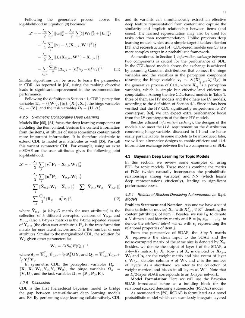
Following the generative process above, thelog-likelihood in Equation (9) becomes:

L =− λu2

∑i

‖ui‖22 −λw2

∑l

(‖Wl‖2F + ‖bl‖22)

− λv2

∑j

‖vj − fe(X0,j∗,W+)T ‖22

− λn2

∑j

‖fr(X0,j∗,W+)−Xc,j∗‖22

−∑i,j,k

Cijk

2(∆ijk − (uTi vj − uTi vk))

2. (11)

Similar algorithms can be used to learn the parametersin CDR. As reported in [64], using the ranking objectiveleads to significant improvement in the recommendationperformance.

Following the definition in Section 4.1, CDR’s perceptionvariables Ωp = Wl, bl, Xl,Xc, the hinge variablesΩh = V, and the task variables Ωt = U,∆.

4.2.5 Symmetric Collaborative Deep LearningModels like [60], [64] focus the deep learning component onmodeling the item content. Besides the content informationfrom the items, attributes of users sometimes contain muchmore important information. It is therefore desirable toextend CDL to model user attributes as well [35]. We callthis variant symmetric CDL. For example, using an extramSDAE on the user attributes gives the following jointlog-likelihood:

L =− λv2

∑j

‖vTj P1 −X0,j∗W1‖22

− λu2

∑i

‖uTi P2 −Y0,j∗W2‖22

−∑j

‖X0,j∗W1 −Xc,j∗‖22 −∑i

‖Y0,i∗W2 −Yc,i∗‖22

−∑i,j

Cij

2(Rij − uTi vj)

2, (12)

where Y0,j∗ (a k-by-D matrix for user attributes) is thecollection of k different corrupted versions of Y0,j∗ andYc,i∗ (also a k-by-D matrix) is the k-time repeated versionof Yc,i∗ (the clean user attributes). P2 is the transformationmatrix for user latent factors and D is the number of userattributes. Similar to the marginalized CDL, the solution forW2 given other parameters is:

W2 = E(S2)E(Q2)−1,

where S2 = YT

c,i∗Y0,i∗+λu2 PT

2 UYc and Q2 = YT

c,i∗Y0,i∗+λu2 YT

c Yc.In symmetric CDL, the perception variables Ωp =

X0,Xc,W1,Y0,Yc,W2, the hinge variables Ωh =V,U, and the task variables Ωt = P1,P2,R.

4.2.6 DiscussionCDL is the first hierarchical Bayesian model to bridgethe gap between state-of-the-art deep learning modelsand RS. By performing deep learning collaboratively, CDL

and its variants can simultaneously extract an effectivedeep feature representation from content and capture thesimilarity and implicit relationship between items (andusers). The learned representation may also be used fortasks other than recommendation. Unlike previous deeplearning models which use a simple target like classification[31] and reconstruction [54], CDL-based models use CF as amore complex target in a probabilistic framework.

As mentioned in Section 1, information exchange betweentwo components is crucial for the performance of BDL.In the CDL-based models above, the exchange is achievedby assuming Gaussian distributions that connect the hingevariables and the variables in the perception component(drawing the hinge variable vj ∼ N (XT

L2 ,j∗

, λ−1v IK) inthe generative process of CDL, where XL

2is a perception

variable), which is simple but effective and efficient incomputation. Among the five CDL-based models in Table 1,three of them are HV models and the others are LV models,according to the definition of Section 4.1. Since it has beenverified that the HV CDL significantly outperforms its ZVcounterpart [60], we can expect extra performance boostfrom the LV counterparts of the three HV models.

Besides efficient information exchange, the designs of themodels also meet the i.i.d. requirement on the distributionconcerning hinge variables discussed in 4.1 and are henceeasily parallelizable. In some models to be introduced later,we will see alternative designs to enable efficient and i.i.d.information exchange between the two components of BDL.

4.3 Bayesian Deep Learning for Topic ModelsIn this section, we review some examples of usingBDL for topic models. These models combine the meritsof PGM (which naturally incorporates the probabilisticrelationships among variables) and NN (which learnsdeep representations efficiently), leading to significantperformance boost.

4.3.1 Relational Stacked Denoising Autoencoders as TopicModelsProblem Statement and Notation: Assume we have a set ofitems (articles or movies) Xc, with XT

c,j∗ ∈ RB denoting thecontent (attributes) of item j. Besides, we use IK to denotea K-dimensional identity matrix and S = [s1, s2, · · · , sJ ] todenote the relational latent matrix with sj representing therelational properties of item j.

From the perspective of SDAE, the J -by-B matrixXc represents the clean input to the SDAE and thenoise-corrupted matrix of the same size is denoted by X0.Besides, we denote the output of layer l of the SDAE, aJ -by-Kl matrix, by Xl. Row j of Xl is denoted by Xl,j∗,Wl and bl are the weight matrix and bias vector of layerl, Wl,∗n denotes column n of Wl, and L is the numberof layers. As a shorthand, we refer to the collection ofweight matrices and biases in all layers as W+. Note thatan L/2-layer SDAE corresponds to an L-layer network.

Model Formulation: Here we will use the BayesianSDAE introduced before as a building block for therelational stacked denoising autoencoder (RSDAE) model.

As mentioned in [59], RSDAE is formulated as a novelprobabilistic model which can seamlessly integrate layered

12

J

x0x0 x2x2 x3x3 x4x4 xcxcx1x1

ss

W+W+

AA ¸l¸l

¸n¸n

¸w¸w

¸r¸r

Fig. 11. Graphical model of RSDAE for L = 4. λs is not shown here toprevent clutter.

representation learning and the relational informationavailable. This way, the model can simultaneously learn thefeature representation from the content information and therelation between items. The graphical model of RSDAE isshown in Figure 11 and the generative process is listed asfollows:

1) Draw the relational latent matrix S from a matrix variatenormal distribution [20]:

S ∼ NK,J(0, IK ⊗ (λlLa)−1). (13)

2) For layer l of the SDAE where l = 1, 2, . . . , L2 − 1,a) For each column n of the weight matrix Wl, draw

Wl,∗n ∼ N (0, λ−1w IKl).b) Draw the bias vector bl ∼ N (0, λ−1w IKl).c) For each row j of Xl, draw

Xl,j∗ ∼ N (σ(Xl−1,j∗Wl + bl), λ−1s IKl).

3) For layer L2 of the SDAE network, draw the

representation vector for item j from the product oftwo Gaussians (PoG) [14]:

XL2 ,j∗∼ PoG(σ(XL

2 −1,j∗Wl + bl), s

Tj , λ

−1s IK , λ

−1r IK).

(14)

4) For layer l of the SDAE network where l = L2 + 1, L2 +

2, . . . , L,a) For each column n of the weight matrix Wl, draw

Wl,∗n ∼ N (0, λ−1w IKl).b) Draw the bias vector bl ∼ N (0, λ−1w IKl).c) For each row j of Xl, draw

Xl,j∗ ∼ N (σ(Xl−1,j∗Wl + bl), λ−1s IKl).

5) For each item j, draw a clean input

Xc,j∗ ∼ N (XL,j∗, λ−1n IB).

Here K = KL2

is the dimensionality of the learnedrepresentation vector for each item, S denotes the K × Jrelational latent matrix in which column j is the relationallatent vector sj for item j. Note thatNK,J(0, IK ⊗ (λlLa)

−1)in Equation (13) is a matrix variate normal distributiondefined as in [20]:

p(S) = NK,J(0, IK ⊗ (λlLa)−1)

=exptr[−λl2 SLaS

T ](2π)JK/2|IK |J/2|λlLa|−K/2

, (15)

where the operator ⊗ denotes the Kronecker product oftwo matrices [20], tr(·) denotes the trace of a matrix, and

La is the Laplacian matrix incorporating the relationalinformation. La = D − A, where D is a diagonal matrixwhose diagonal elements Dii =

∑j Aij and A is the

adjacency matrix representing the relational informationwith binary entries indicating the links (or relations)between items. Ajj′ = 1 indicates that there is a linkbetween item j and item j′ and Ajj′ = 0 otherwise.PoG(σ(XL

2 −1,j∗Wl + bl), s

Tj , λ

−1s IK , λ

−1r IK) denotes the

product of the Gaussian N (σ(XL2 −1,j∗

Wl + bl), λ−1s IK)

and the Gaussian N (sTj , λ−1r IK), which is also a Gaussian

[14].According to the generative process above, maximizing

the posterior probability is equivalent to maximizing thejoint log-likelihood of Xl, Xc, S, Wl, and bl givenλs, λw, λl, λr , and λn:

L =− λl2tr(SLaS

T )− λr2

∑j

‖(sTj −XL2 ,j∗

)‖22

− λw2

∑l

(‖Wl‖2F + ‖bl‖22)

− λn2

∑j

‖XL,j∗ −Xc,j∗‖22

− λs2

∑l

∑j

‖σ(Xl−1,j∗Wl + bl)−Xl,j∗‖22.

Similar to the generalized SDAE, taking λs to infinity,the joint log-likelihood becomes:

L =− λl2tr(SLaS

T )− λr2

∑j

‖(sTj −XL2 ,j∗

)‖22

− λw2

∑l

(‖Wl‖2F + ‖bl‖22)

− λn2

∑j

‖XL,j∗ −Xc,j∗‖22, (16)

where Xl,j∗ = σ(Xl−1,j∗Wl + bl). Note that the firstterm −λl2 tr(SLaS

T ) corresponds to log p(S) in the matrixvariate distribution in Equation (15). Besides, by simple

manipulation, we have tr(SLaST ) =

K∑k=1

STk∗LaSk∗, where

Sk∗ denotes the k-th row of S. As we can see, maximizing−λl2 tr(S

TLaS) is equivalent to making sj closer to sj′ ifitem j and item j′ are linked (namely Ajj′ = 1).

In RSDAE, the perception variables Ωp =Xl,Xc, Wl, bl, the hinge variables Ωh = S,and the task variables Ωt = A.

Learning Relational Representation and Topics: [59]provides an EM-style algorithm for MAP estimation. Herewe review some of the key steps as follows.

In terms of the relational latent matrix S, we first fix allrows of S except the k-th one Sk∗ and then update Sk∗.Specifically, we take the gradient of L with respect to Sk∗,set it to 0, and get the following linear system:

(λlLa + λrIJ)Sk∗ = λrXTL2 ,∗k

. (17)

A naive approach is to solve the linear system bysetting Sk∗ = λr(λlLa + λrIJ)

−1XTL2 ,∗k

. Unfortunately,the complexity is O(J3) for one single update. Similar to

13

[36], the steepest descent method [50] is used to iterativelyupdate Sk∗:

Sk∗(t+ 1)← Sk∗(t) + δ(t)r(t)

r(t)← λrXTL2 ,∗k− (λlLa + λrIJ)Sk∗(t)

δ(t)← r(t)T r(t)

r(t)T (λlLa + λrIJ)r(t).

As discussed in [36], the use of steepest descent methoddramatically reduces the computation cost in each iterationfrom O(J3) to O(J).

Given S, we can learn Wl and bl for each layer usingthe back-propagation algorithm. By alternating the updateof S, Wl, and bl, a local optimum for L can be found. Also,techniques such as including a momentum term may helpto avoid being trapped in a local optimum.

4.3.2 Deep Poisson Factor Analysis with Sigmoid BeliefNetworks

The Poisson distribution with support over nonnegativeintegers is known as a natural choice to model counts. Itis, therefore, desirable to use it as a building block for topicmodels [6]. With this motivation, [66] proposed a model,dubbed Poisson factor analysis (PFA), for latent nonnegativematrix factorization via Poisson distributions.

Poisson Factor Analysis: PFA assumes a discreteP -by-N matrix X containing word counts of N documentswith a vocabulary size of P [15], [66]. In a nutshell, PFA canbe described using the following equation:

X ∼ Pois(Φ(Θ H)), (18)

where Φ (of size P -by-K where K is the number of topics)denotes the factor loading matrix in factor analysis with thek-th column φk encoding the importance of each word intopic k. The K-by-N matrix Θ is the factor score matrixwith the n-th column θn containing topic proportions fordocument n. The K-by-N matrix H is a latent binary matrixwith the n-th column hn defining a set of topics associatedwith document n.

Different priors correspond to different models. Forexample, Dirichlet priors on φk and θn with an all-onematrix H would recover LDA [6] while a beta-Bernoulliprior on hn leads to the NB-FTM model in [65]. In [15],a deep-structured prior based on sigmoid belief networks(SBN) [39] (an MLP variant with binary hidden units)is imposed on hn to form a deep PFA model for topicmodeling.

Deep Poisson Factor Analysis: In the deep PFA model

[15], the generative process can be summarized as follows:

φk ∼ Dir(aφ, . . . , aφ)

θkn ∼ Gamma(rk,pn

1− pn)

rk ∼ Gamma(γ0,1

c0)

γ0 ∼ Gamma(e0,1

f0)

h(L)kLn∼ Ber(σ(b(L)kL

)) (19)

h(l)kln∼ Ber(σ(w(l)

kl

Th(l+1)n + b

(l)kl)) (20)

xpnk ∼ Pois(φpkθknh(1)kn ) (21)

xpn =K∑k=1

xpnk,

where L is the number of layers in SBN, which correspondsto Equation (19) and (20). xpnk is the count of word p thatcomes from topic k in document n.

In this model, the perception variables Ωp =H(l), Wl, bl, the hinge variables Ωh = X, andthe task variables Ωt = φk, rk,Θ, γ0. Wl is theweight matrix containing columns of w

(l)kl

and bl is the biasvector containing entries of b(l)kl in Equation (20).

Learning Using Bayesian Conditional DensityFiltering: Efficient learning algorithms are needed forBayesian treatments of deep PFA. [15] proposed to usean online version of MCMC called Bayesian conditionaldensity filtering (BCDF) to learn both the global parametersΨg = (φk, rk, γ0, Wl, bl) and the local variablesΨl = (Θ, H(l)). The key conditional densities used forthe Gibbs updates are as follows:

xpnk|− ∼ Multi(xpn; ζpn1, . . . , ζpnK)

φk|− ∼ Dir(aφ + x1·k, . . . , aφ + xP ·k)

θkn|− ∼ Gamma(rkh(1)kn + x·nk, pn)

h(1)kn |− ∼ δ(x·nk = 0)Ber(

πknπkn + (1− πkn)

) + δ(x·nk > 0),

where πkn = πkn(1 − pn)rk , πkn = σ((w(1)k )Th

(2)n + c

(1)k ),

x·nk =P∑p=1

xpnk, xp·k =N∑n=1

xpnk, and ζpnk ∝ φpkθkn. For

the learning of h(l)kn where l > 1, the same techniques as in[16] can be used.

Learning Using Stochastic Gradient Thermostats: Analternative way of learning deep PFA is through the use ofstochastic gradient Nose-Hoover thermostats (SGNHT), whichis more accurate and scalable. SGNHT is a generalization ofthe stochastic gradient Langevin dynamics (SGLD) [63] and thestochastic gradient Hamiltonian Monte Carlo (SGHMC) [11].Compared with the previous two, it introduces momentumvariables into the system, helping the system to jumpout of local optima. Specifically, the following stochasticdifferential equations (SDE) can be used:

dΨg = vdt

dv = f(Ψg)dt− ξvdt+√DdW

dξ = (1

MvTv − 1)dt,

14

where f(Ψg) = −∇ΨgU(Ψg) and U(Ψg) is the negative

log-posterior of the model. t indexes time and W denotesthe standard Wiener process. ξ is the thermostats variableto make sure the system has a constant temperature. Dis the injected variance which is a constant. To speed upconvergence, the SDE is generalized to:

dΨg = vdt

dv = f(Ψg)dt−Ξvdt+√DdW

dΞ = (q− I)dt,

where I is the identity matrix, Ξ = diag(ξ1, . . . , ξM ),q = diag(v21 , . . . , v

2M ), and M is the dimensionality of the

parameters.

4.3.3 Deep Poisson Factor Analysis with RestrictedBoltzmann MachineSimilar to the deep PFA above, the restricted Boltzmannmachine (RBM) [23] can be used in place of SBN [15]. If RBMis used, Equation (19) and (20) would be defined using theenergy [23]:

E(h(l)n ,h

(l+1)n ) =− (h(l)

n )T c(l) − (h(l)n )TW(l)h(l+1)

n

− (h(l+1)n )T c(l+1).

For the learning, similar algorithms as the deep PFA withSBN can be used. Specifically, the sampling process wouldalternate between φk, γk, γ0 and W(l), c(l).For the former, similar conditional density as the SBN-basedDPFA is used. For the latter, they use the contrastivedivergence algorithm.

4.3.4 DiscussionIn BDL-based topic models, the perception componentis responsible for inferring the topic hierarchy fromdocuments while the task-specific component is in charge ofmodeling the word generation, topic generation, word-topicrelation, or inter-document relation. The synergy betweenthese two components comes from the bidirectionalinteraction between them. On one hand, knowledge on thetopic hierarchy would facilitate accurate modeling of wordsand topics, providing valuable information for learninginter-document relation. On the other hand, accuratelymodeling the words, topics, and inter-document relationcould help with the discovery of topic hierarchy andlearning of compact document representations.

As we can see, the information exchange mechanism insome BDL-based topic models is different from that inSection 4.2. For example, in the SBN-based DPFA model,the exchange is natural since the bottom layer of SBN, H(1),and the relationship between H(1) and Ωh = X are bothinherently probabilistic, as shown in Equation (20) and (21),which means additional assumptions on the distribution arenot necessary. The SBN-based DPFA model is equivalent toassuming that H in PFA (see Equation (18)) is generatedfrom a Dirac delta distribution (a Gaussian distribution withzero variance) centered at the bottom layer of the SBN,H(1). Hence both DPFA models in Table 1 are ZV models,according to the definition in Section 4.1. It is worth notingthat RSDAE is an HV model (see Equation (14), where S isthe hinge variable and the others are perception variables),

and naively modifying this model to be its ZV counterpartwould violate the i.i.d. requirement in Section 4.1.

4.4 Bayesian Deep Learning for ControlAs mentioned in Section 1, Bayesian deep learning can alsobe applied to the control of nonlinear dynamical systemsfrom raw images. Consider controlling a complex dynamicalsystem according to the live video stream received froma camera. One way of solving this control problem is byiteration between two tasks, perception from raw imagesand control based on dynamic models. The perceptiontask can be taken care of using multiple layers of simplenonlinear transformation (deep learning) while the controltask usually needs more sophisticated models like hiddenMarkov models and Kalman filters [21], [38]. To enable aneffective iterative process between the perception task andthe control task, we need two-way information exchangebetween them. The perception component would be thebasis on which the control component estimates its statesand on the other hand, the control component with adynamic model built in would be able to predict the futuretrajectory (images) by reversing the perception process [62].

4.4.1 Stochastic Optimal ControlFollowing [62], we consider the stochastic optimal control ofan unknown dynamical system as follows:

zt+1 = f(zt,ut) + ξ, ξ ∼ N (0,Σξ), (22)

where t indexes the time steps and zt ∈ Rnz isthe latent states. ut ∈ Rnu is the applied control attime t and ξ denotes the system noise. Equivalently,the equation above can be written as P (zt+1|zt,ut) =N (zt+1|f(zt,ut),Σξ). Hence we need a mapping functionto map the corresponding raw image xt (observed input)into the latent space:

zt = m(xt) + ω, ω ∼ N (0,Σω),

where ω is the corresponding system noise. Similarly theequation above can be rewritten as zt ∼ N (m(xt),Σω).If the function f is given, finding optimal control for atrajectory of length T in a dynamical system amounts tominimizing the following cost:

J(z1:T ,u1:T ) = Ez(cT (zT ,uT ) +T−1∑t0

c(zt,ut)), (23)

where cT (zT ,uT ) is the terminal cost and c(zt,ut)is the instantaneous cost. z1:T = z1, . . . , zT andu1:T = u1, . . . ,uT are the state and action sequences,respectively. For simplicity we can let cT (zT ,uT ) =c(zT ,uT ) and use the following quadratic cost:

c(zt,ut) = (zt − zgoal)TRz(zt − zgoal) + uTt Ruut,

where Rz ∈ Rnz×nz and Ru ∈ Rnu×nu are the weightingmatrices. zgoal is the target latent state that should beinferred from the raw images (observed input). Given thefunction f , z1:T (current estimates of the optimal trajectory),and u1:T (the corresponding controls), the dynamicalsystem can be linearized as:

zt+1 = A(zt)zt + B(zt)ut + o(zt) + ω, ω ∼ N (0,Σω),(24)

15

where A(zt) = ∂f(zt,ut)∂zt

and B(zt) = ∂f(zt,ut)∂ut

are localJacobians. o(zt) is the offset.

4.4.2 BDL-Based ControlTo minimize the function in Equation (23), we need threekey components: an encoding model to encode xt intozt, a transition model to infer zt+1 given (zt,ut), and areconstruction model to reconstruct xt+1 from the inferredzt+1.

Encoding Model: An encoding model Qφ(Z|X) =N (µt,diag(σ2

t )), where the mean µt ∈ Rnz and thediagonal covariance Σt = diag(σ2

t ) ∈ Rnz×nz , encodes theraw images xt into latent states zt. Here,

µt = Wµhencφ (xt) + bµ (25)

logσt = Wσhencφ (xt) + bσ, (26)

where hφ(xt)enc is the output of the encoding network withxt as its input.

Transition Model: A transition model like Equation (24)infers zt+1 from (zt,ut). If we use Qψ(Z|Z,u) to denotethe approximate posterior distribution to generate zt+1, thegenerative process of the full model would be:

zt ∼ Qφ(Z|X) = N (µt,Σt) (27)

zt+1 ∼ Qψ(Z|Z,u) = N (Atµt + Btut + ot,Ct)(28)

xt, xt+1 ∼ Pθ(X|Z) = Bernoulli(pt), (29)

where Equation (29) is the reconstruction model to bediscussed later, Ct = AtΣtA

Tt + Ht, and Ht is the

covariance matrix of the estimated system noise (ωt ∼N (0,Ht)). The key here is to learn At, Bt and ot, whichare parameterized as follows:

vec(At) = WAhtransψ (zt) + bA

vec(Bt) = WBhtransψ (zt) + bB

ot = Wohtransψ (zt) + bo,

where htransψ (zt) is the output of the transition network.

Reconstruction Model: As mentioned in Equation (29),the posterior distribution Pθ(X|Z) reconstructs the rawimages xt from the latent states zt. In Equation (29), theparameters for the Bernoulli distribution pt = Wph

decθ (zt)+

bp where hdecθ (zt) is the output of a third network, called the

decoding network or the reconstruction network. Putting itall together, Equation (27)-(29) show the generative processof the full model.

4.4.3 Learning Using Stochastic Gradient VariationalBayesWith D = (x1,u1,x2), . . . , (xT−1,uT−1,xT ) as thetraining set, the loss function is as follows:

L =∑

(xt,ut,xt+1)∈D

Lbound(xt,ut,xt+1)

+ λ KL(Qψ(Z|µt,ut)‖Qφ(Z|xt+1)),

where the first term is the variational bound on themarginalized log-likelihood for each data point:

Lbound(xt,ut,xt+1) = E zt∼Qφzt+1∼Qψ

(− logPθ(xt|zt)

− logPθ(xt+1|zt+1)) + KL(Qφ‖P (Z)),

where P (Z) is the prior distribution for Z. With theequations above, stochastic gradient variational Bayes canbe used to learn the parameters.

According to the generative process in Equation(27)-(29) and the definition in Section 4.1, the perceptionvariables Ωp = henc

φ (·),W+p ,xt,µt,σt,pt, h

decθ (·), where

W+p is shorthand for Wµ,bµ,Wσ,bσ,Wp,bp. The

hinge variables Ωh = zt, zt+1 and the task variablesΩt = At,Bt,ot,ut,Ct,ωt,W

+t , h

transψ (·), where W+

t isshorthand for WA,bA,WB ,bB ,Wo,bo.

4.4.4 DiscussionAs mentioned in Section 1, BDL-based control modelsconsist of two components, a perception component to seethe live video and a control (task-specific) component toinfer the states of the dynamical system. Inference of thesystem is based on the mapped states and the confidenceof mapping from the perception component, and in return,the control signals sent by the control component wouldaffect the live video received by the perception component.Only when the two components work interactively within aunified probabilistic framework can the model reach its fullpotential and achieve the best control performance.

In terms of information exchange between the twocomponents, the BDL-based control model discussed aboveuses a different mechanism from Section 4.2 and Section 4.3:it uses neural networks to separately parameterize the meanand covariance of hinge variables (e.g., in the encodingmodel, the hinge variable zt ∼ N (µt,diag(σ2

t )), whereµt and σt are perception variables parameterized as inEquation (25) and (26)), which is more flexible (with morefree parameters) than models like CDL and CDR in Section4.2, where Gaussian distributions with fixed variance arealso used. Note that this BDL-based control model is anLV model as shown in Table 1, and since the covarianceis assumed to be diagonal, the model still meets the i.i.d.requirement in Section 4.1.

5 CONCLUSIONS AND FUTURE RESEARCH

In this survey, we identified a current trend of mergingprobabilistic graphical models and neural networks (deeplearning) and reviewed recent work on Bayesian deeplearning, which strives to combine the merits of PGM andNN by organically integrating them in a single principledprobabilistic framework. To learn parameters in BDL,several algorithms have been proposed, ranging from blockcoordinate descent, Bayesian conditional density filtering,and stochastic gradient thermostats to stochastic gradientvariational Bayes.

Bayesian deep learning gains its popularity both fromthe success of PGM and from the recent promising advanceson deep learning. Since many real-world tasks involveboth perception and inference, BDL is a natural choice toharness the perception ability from NN and the (causaland logical) inference ability from PGM. Although currentapplications of BDL focus on recommender systems, topicmodels, and stochastic optimal control, in the future, wecan expect an increasing number of other applicationslike link prediction, community detection, active learning,Bayesian reinforcement learning, and many other complex

16

tasks that need interaction between perception and causalinference. Besides, with the advances of efficient Bayesianneural networks (BNN), BDL with BNN as an importantcomponent is expected to be more and more scalable.

REFERENCES

[1] Anoop Korattikara Balan, Vivek Rathod, Kevin P Murphy, andMax Welling. Bayesian dark knowledge. In NIPS, pages3420–3428, 2015.

[2] Yoshua Bengio, Li Yao, Guillaume Alain, and Pascal Vincent.Generalized denoising auto-encoders as generative models. InNIPS, pages 899–907, 2013.

[3] Christopher M. Bishop. Pattern Recognition and Machine Learning.Springer-Verlag New York, Inc., Secaucus, NJ, USA, 2006.

[4] David Blei and John Lafferty. Correlated topic models. NIPS,18:147, 2006.

[5] David M Blei and John D Lafferty. Dynamic topic models. InICML, pages 113–120. ACM, 2006.

[6] David M Blei, Andrew Y Ng, and Michael I Jordan. LatentDirichlet allocation. JMLR, 3:993–1022, 2003.

[7] Charles Blundell, Julien Cornebise, Koray Kavukcuoglu, and DaanWierstra. Weight uncertainty in neural network. In ICML, pages1613–1622, 2015.

[8] Herve Bourlard and Yves Kamp. Auto-association by multilayerperceptrons and singular value decomposition. Biologicalcybernetics, 59(4-5):291–294, 1988.

[9] Minmin Chen, Kilian Q Weinberger, Fei Sha, and YoshuaBengio. Marginalized denoising auto-encoders for nonlinearrepresentations. In ICML, pages 1476–1484, 2014.

[10] Minmin Chen, Zhixiang Eddie Xu, Kilian Q. Weinberger, and FeiSha. Marginalized denoising autoencoders for domain adaptation.In ICML, 2012.

[11] Tianqi Chen, Emily B. Fox, and Carlos Guestrin. Stochasticgradient Hamiltonian Monte Carlo. In ICML, pages 1683–1691,2014.

[12] Kyunghyun Cho, Bart van Merrienboer, cCaglar Gulccehre,Dzmitry Bahdanau, Fethi Bougares, Holger Schwenk, andYoshua Bengio. Learning phrase representations using RNNencoder-decoder for statistical machine translation. In EMNLP,pages 1724–1734, 2014.

[13] Yarin Gal and Zoubin Ghahramani. Dropout as a Bayesianapproximation: Insights and applications. In Deep LearningWorkshop, ICML, 2015.

[14] M. J. F. Gales and S. S. Airey. Product of Gaussians for speechrecognition. CSL, 20(1):22–40, 2006.

[15] Zhe Gan, Changyou Chen, Ricardo Henao, David E. Carlson, andLawrence Carin. Scalable deep Poisson factor analysis for topicmodeling. In ICML, pages 1823–1832, 2015.

[16] Zhe Gan, Ricardo Henao, David E. Carlson, and Lawrence Carin.Learning deep sigmoid belief networks with data augmentation.In AISTATS, 2015.

[17] Kostadin Georgiev and Preslav Nakov. A non-iid framework forcollaborative filtering with restricted Boltzmann machines. InICML, pages 1148–1156, 2013.

[18] Ian Goodfellow, Yoshua Bengio, and Aaron Courville. DeepLearning. Book in preparation for MIT Press, 2016.

[19] Alex Graves. Practical variational inference for neural networks.In NIPS, pages 2348–2356, 2011.

[20] A.K. Gupta and D.K. Nagar. Matrix Variate Distributions. Chapman& Hall/CRC Monographs and Surveys in Pure and AppliedMathematics. Chapman & Hall, 2000.

[21] Jeff Harrison and Mike West. Bayesian Forecasting & DynamicModels. Springer, 1999.

[22] Jose Miguel Hernandez-Lobato and Ryan Adams. Probabilisticbackpropagation for scalable learning of bayesian neuralnetworks. In ICML, pages 1861–1869, 2015.

[23] Geoffrey E. Hinton. Training products of experts by minimizingcontrastive divergence. Neural Computation, 14(8):1771–1800, 2002.

[24] Geoffrey E Hinton and Drew Van Camp. Keeping the neuralnetworks simple by minimizing the description length of theweights. In COLT, pages 5–13, 1993.

[25] Geoffrey E Hinton and Richard S Zemel. Autoencoders, minimumdescription length, and Helmholtz free energy. NIPS, pages 3–3,1994.

[26] Matthew Hoffman, Francis R Bach, and David M Blei. Onlinelearning for latent Dirichlet allocation. In NIPS, pages 856–864,2010.

[27] Matthew D. Hoffman, David M. Blei, Chong Wang, andJohn William Paisley. Stochastic variational inference. JMLR,14(1):1303–1347, 2013.

[28] Yifan Hu, Yehuda Koren, and Chris Volinsky. Collaborativefiltering for implicit feedback datasets. In ICDM, pages 263–272,2008.

[29] David H Hubel and Torsten N Wiesel. Receptive fields andfunctional architecture of monkey striate cortex. The Journal ofphysiology, 195(1):215–243, 1968.

[30] Michael I. Jordan, Zoubin Ghahramani, Tommi Jaakkola, andLawrence K. Saul. An introduction to variational methods forgraphical models. Machine Learning, 37(2):183–233, 1999.

[31] Nal Kalchbrenner, Edward Grefenstette, and Phil Blunsom. Aconvolutional neural network for modelling sentences. ACL, pages655–665, 2014.

[32] Diederik P Kingma and Max Welling. Auto-encoding variationalbayes. arXiv preprint arXiv:1312.6114, 2013.

[33] Y. LeCun. Modeles connexionnistes de l’apprentissage (connectionistlearning models). PhD thesis, Universite P. et M. Curie (Paris 6),June 1987.

[34] Yann LeCun, Leon Bottou, Yoshua Bengio, and Patrick Haffner.Gradient-based learning applied to document recognition.Proceedings of the IEEE, 86(11):2278–2324, 1998.

[35] Sheng Li, Jaya Kawale, and Yun Fu. Deep collaborative filteringvia marginalized denoising auto-encoder. In CIKM, pages 811–820,2015.

[36] Wu-Jun Li and Dit-Yan Yeung. Relation regularized matrixfactorization. In IJCAI, 2009.

[37] JC MacKay David. A practical Bayesian framework for backpropnetworks. Neural computation, 1992.

[38] Takamitsu Matsubara, Vicencc Gomez, and Hilbert J. Kappen.Latent Kullback Leibler control for continuous-state systems usingprobabilistic graphical models. In UAI, pages 583–592, 2014.

[39] Radford M. Neal. Connectionist learning of belief networks. Artif.Intell., 56(1):71–113, 1992.

[40] Radford M Neal. Bayesian learning for neural networks. PhD thesis,University of Toronto, 1995.

[41] Aaron Van Den Oord, Sander Dieleman, and BenjaminSchrauwen. Deep content-based music recommendation. In NIPS,pages 2643–2651, 2013.

[42] Ian Porteous, David Newman, Alexander Ihler, Arthur Asuncion,Padhraic Smyth, and Max Welling. Fast collapsed gibbs samplingfor latent Dirichlet allocation. In KDD, pages 569–577, 2008.

[43] Christopher Poultney, Sumit Chopra, Yann L Cun, et al. Efficientlearning of sparse representations with an energy-based model. InNIPS, pages 1137–1144, 2006.

[44] Sanjay Purushotham, Yan Liu, and C.-C. Jay Kuo. Collaborativetopic regression with social matrix factorization forrecommendation systems. In ICML, pages 759–766, 2012.

[45] Francesco Ricci, Lior Rokach, and Bracha Shapira. Introduction toRecommender Systems Handbook. Springer, 2011.

[46] Salah Rifai, Pascal Vincent, Xavier Muller, Xavier Glorot, andYoshua Bengio. Contractive auto-encoders: Explicit invarianceduring feature extraction. In ICML, pages 833–840, 2011.

[47] Tara N. Sainath, Brian Kingsbury, Vikas Sindhwani, Ebru Arisoy,and Bhuvana Ramabhadran. Low-rank matrix factorizationfor deep neural network training with high-dimensional outputtargets. In ICASSP, pages 6655–6659, 2013.

[48] Ruslan Salakhutdinov and Andriy Mnih. Probabilistic matrixfactorization. In NIPS, pages 1257–1264, 2007.

[49] Ruslan Salakhutdinov, Andriy Mnih, and Geoffrey E. Hinton.Restricted Boltzmann machines for collaborative filtering. InICML, pages 791–798, 2007.

[50] Jonathan R Shewchuk. An introduction to the conjugate gradientmethod without the agonizing pain. Technical report, CarnegieMellon University, Pittsburgh, PA, USA, 1994.

[51] Nitish Srivastava, Geoffrey Hinton, Alex Krizhevsky, IlyaSutskever, and Ruslan Salakhutdinov. Dropout: A simple way toprevent neural networks from overfitting. JMLR, 15(1):1929–1958,2014.

[52] Robert S Strichartz. A Guide to Distribution Theory and FourierTransforms. World Scientific, 2003.

17

[53] Ilya Sutskever, Oriol Vinyals, and Quoc VV Le. Sequenceto sequence learning with neural networks. In NIPS, pages3104–3112, 2014.

[54] Pascal Vincent, Hugo Larochelle, Isabelle Lajoie, Yoshua Bengio,and Pierre-Antoine Manzagol. Stacked denoising autoencoders:Learning useful representations in a deep network with a localdenoising criterion. JMLR, 11:3371–3408, 2010.

[55] Chong Wang and David M. Blei. Collaborative topic modeling forrecommending scientific articles. In KDD, pages 448–456, 2011.

[56] Chong Wang, David M. Blei, and David Heckerman. Continuoustime dynamic topic models. In UAI, pages 579–586, 2008.

[57] Hao Wang, Binyi Chen, and Wu-Jun Li. Collaborative topicregression with social regularization for tag recommendation. InIJCAI, pages 2719–2725, 2013.

[58] Hao Wang and Wu-Jun Li. Relational collaborative topicregression for recommender systems. TKDE, 27(5):1343–1355,2015.

[59] Hao Wang, Xingjian Shi, and Dit-Yan Yeung. Relational stackeddenoising autoencoder for tag recommendation. In AAAI, pages3052–3058, 2015.

[60] Hao Wang, Naiyan Wang, and Dit-Yan Yeung. Collaborative deeplearning for recommender systems. In KDD, pages 1235–1244,2015.

[61] Xinxi Wang and Ye Wang. Improving content-based and hybridmusic recommendation using deep learning. In ACM MM, pages627–636, 2014.

[62] Manuel Watter, Jost Springenberg, Joschka Boedecker, and MartinRiedmiller. Embed to control: A locally linear latent dynamicsmodel for control from raw images. In NIPS, pages 2728–2736,2015.

[63] Max Welling and Yee Whye Teh. Bayesian learning via stochasticgradient langevin dynamics. In ICML, pages 681–688, 2011.

[64] Haochao Ying, Liang Chen, Yuwen Xiong, and Jian Wu.Collaborative deep ranking: a hybrid pair-wise recommendationalgorithm with implicit feedback. In PAKDD, 2016.

[65] Mingyuan Zhou and Lawrence Carin. Negative binomial processcount and mixture modeling. IEEE Trans. Pattern Anal. Mach.Intell., 37(2):307–320, 2015.

[66] Mingyuan Zhou, Lauren Hannah, David B. Dunson, andLawrence Carin. Beta-negative binomial process and Poissonfactor analysis. In AISTATS, pages 1462–1471, 2012.