1 visions - vista star formation atlas - eso · 1 visions - vista star formation atlas pi: j....

ESO Survey Management Plan Form Phase 1

1 VISIONS - VISTA Star Formation Atlas

PI: J. Alves, University of Vienna, AustriaCo-PIs: S. Meingast, University of Vienna, Austria; H. Bouy, University of Bordeaux, France

CoIs: M. Lombardi, Italy; J. Ascenso, Portugal; A. Bayo, Chile; E. Bertin, France; A.Brown, The Netherlands; Jos de Bruijne, ESA; J. Forbrich, Austria; J. Großschedl, Aus-tria; A. Hacar, The Netherlands; B. Hasenberger, Austria; J. Kainulainen, Germany; J.Kauffmann, Germany; R. Kohler, Austria; K. Kubiak, Austria; K. Leschinski, Austria, D.Mardones, Chile; A. Moitinho, Portugal; K. Pena Ramırez, Chile; M. Petr-Gotzens, ESO;T. Prusti, ESA; L. Sarro, Spain; T. Robitaille, Germany; R. Ramlau, Austria; R. Schodel,Spain; P. Teixeira, Austria; E. Zari, The Netherlands; W. Zeilinger, Austria;

1.1 Abstract

The VISTA Star Formation Atlas (VISIONS) is a sub-arcsec near-infrared atlas of all nearby (d < 500 pc) starformation complexes accessible from the southern hemisphere. This atlas will become the community’s referencestar formation database, covering the mass spectrum down to a few Jupiter masses and spatial resolutionsreaching 100-250 AU. The survey will cover a total of ∼550 deg2 distributed over the six star forming complexesof Ophiuchus, Lupus, Corona Australis, Chamaeleon, Orion, and the Pipe Nebula and is planned to be finishedthree years after the observations commence. VISIONS is separated into three sub-surveys. A wide astrometricsurvey will perform large-scale H-band imaging of the target regions distributed over six epochs with an effectiveexposure time of 60s and a limiting magnitude of H ≈ 19 mag. The immediate objective of the wide surveyis to derive positions and proper motions of the embedded and dispersed young stellar population inaccessibleto Gaia, as well as provide complementary photometry to the first generation VHS survey which fully coveredall target regions in the J and KS bands. The total requested time for the wide multi-epoch survey amounts478h 41m 36s distributed over 2148 individual tiles. Complementary to the wide survey VISIONS includes aset of deep observations which will image the high-column density regions of the star-forming complexes. Thedeep survey features JHKS observations of 57 tiles imaged in one epoch and 600s exposure times including skyoffsets reaching limiting magnitudes of J ≈ 21.5 mag, H ≈ 20.5 mag, and KS ≈ 19.5 mag. The total requestedtime for the deep survey amounts 54h 36m 36s. For statistical comparison with the galactic field populationVISIONS includes a set of six control fields (18 tiles) with the same limiting magnitudes and similar strategy asthe deep observations. For the control sub-survey the requested observing time amounts 19h 19m 12s. In totalthe requested time for VISIONS amounts 552h 37m 24s for 2223 tiles where for the majority Thin observingconditions are required.

2 Survey Observing Strategy

VISIONS, the VISTA Star Formation Atlas, will allow the community to address in a complete and coherentway fundamental open questions in star formation and ISM research. The VISIONS public survey, optimizedfor astrometry, aims to observe all molecular cloud complexes within 500 pc accessible from the southernhemisphere. To achieve its goals, the following observing strategy, calling for three sub-surveys, was designed:we will observe 1) wide fields, covering the poorly known dispersed young population, 2) deep fields in thehigh-column density regions in these complexes (AV > 5 magnitudes), where sensitivity and resolution are keyto recover the embedded population of protostars, and 3) critical but often forgotten control fields.

A detailed view on both the wide and deep target regions is shown in Fig. 1 which also shows the coverageof other public VISTA surveys. An overview of the observing strategies and time requests for all sub-surveysis given in Tab. 1. The table lists - for each region and sub-survey the number of requested tiles, coveredarea, observing sequence, as well as individual and total OB execution times. For all sub-surveys in common a

ESO-USD ([email protected]) page 1 of 22


VHS-NGC

VHS-GPS (north)

VHS-GPS (south)

VHS-SGC

VVVX

90° 0° 270°

60°

30°

0°

-30°

-60°

Gala

ctic

Lati

tude

Orion

VISIONVISTA SV

220° 210° 200°

-15°

-20°

-25°

-30°

Gala

ctic

Lati

tude

Corona Australis

5° 0° 355° 350°

-15°

-20°

Chamaeleon

310° 300° 290°

-5°

-10°

-15°

-20°

Galactic Longitude

Gala

ctic

Lati

tude

Ophiuchus/Pipe/Lupus

0° 345° 330°

20°

10°

Galactic Longitude

0 1 2 3AV (mag)

Figure 1: Overview of all wide (blue) and deep (red) target regions. The limits of the public VISTA surveysVVVX (black dashed lines) and VHS (green solid lines) are also displayed.



1 arcmin overlap for the doubly exposed area in a VISTA tile is included for adjacent tiles.

2.1 VISIONS sub-surveys

In the following subsections we will individually discuss the survey observing strategies in more detail for thethree independent sub-surveys. In addition to the figures and tables presented in this document, we also offeran interactive display of the survey field definitions via the Aladin Sky Atlas (Bonnarel et al., 2000)1. Userscan start the Aladin Sky Atlas and load the survey script by entering the following line into the command barat the top of the software window (it is recommended to allow the software a few seconds to finish the scriptwhile the VISIONS coverage is drawn):

load https://www.univie.ac.at/alveslab/VISIONS/coverage.ajs

The resulting view shows all current field definitions on top of the Planck R2 HFI color composite (353-545-857GHz). Wide tiles are shown with blue contours, deep tiles with red contours, and control tiles with greencontours. For each tile the center position of all offsets are displayed, excluding jittered pointings. In additionalso the VVVX, VISTA Science Verification, and the Meingast et al. (2016) Orion A VISTA observation contoursare shown.

2.1.1 Wide sub-survey

The wide sub-survey features large-scale observations over six epochs of the nearby star forming regions Ophi-uchus, Lupus, Corona Australis, Chamaeleon, and Orion. As agreed with the PSP, the wide field for the Pipenebula was omitted since this region will be covered by the parallel ongoing public VVVX survey. The maingoals of the wide observations are to provide complementary information on positions and proper motions forsources inaccessible to Gaia and deep near-infrared photometry on large scales. This includes both the embed-ded protostellar population of the star forming complexes, as well as the more evolved and dispersed youngstars and brown dwarfs. The goals in choosing these wide fields were to cover as much as possible of the (a) highcolumn-density parts of the cloud, (b) the very young embedded objects, as well as (c) the more dispersed youngstellar population.

All regions are to be observed in H-band to provide complementary data to the first generation public VHSsurvey which imaged all our target regions in the J and KS bands. In addition, the VHS survey will allowto extend the time-baseline for derived proper motions. For 60s per pixel effective exposure time on theassembled tiles we chose a combination of DIT= 3s, NDIT= 2, NJITTER= 5 resulting in a single OB executiontime of 14m 12s. While this setup will saturate stars brighter than H ≈ 11.7 mag, we expect to reach acompleteness of around H ≈ 19 mag. Since the low order wave-front sensor imposes a minimum of 45s betweenindividual jittered exposures, the observations must necessarily be taken in open-AO mode with AO correctionsonly between exposures. Given these short integration times we will switch the priority of the active opticscorrections to “low” if necessary to retain the same OB execution times. As recommended by the EST we willadditionally set AG=T for the first pawprint of the sequence to minimize ellipticity due to the short integrationtimes.

Based on our experience with the Meingast et al. (2016) data we chose a number of five jittered positions toensure adequate bad pixel rejection for accurate positional measurements. In order to optimize the surveyefficiency 4 adjacent tiles will be merged into a concatenation. After the first OB execution in a concatenation,subsequent executions will take only 12m 32s. Thus, for 4 concatenated OBs, the average OB time amounts12m 57s, the total time 51m 48s. To optimize the positional measurements over the duration of the survey anddistribute the different epochs, we will define absolute time intervals for the different sets of concatenated OBs(see Sect. 2.2.1 for details).

The total area covered in the wide survey is 537.4 deg2 distributed over 358 individual tiles. For the planned sixepochs there are then a total of 2148 tiles to be observed. 2/3 of the OBs (1440) will be put into concatenation

1Available for download via http://aladin.u-strasbg.fr


http://aladin.u-strasbg.fr


containers, while we leave one third (708) as single OBs to be efficiently scheduled between observations or atthe end of the night. The wide sub-survey will take up the largest fraction of the requested observing time witha total of 478h 41m 36s.

2.1.2 Deep sub-survey

Deep field observations in addition to the wide astrometric survey will image the high-column density partsof nearby star-forming regions in the J , H, and KS bands. The largest clouds (Orion A and B) have alreadybeen observed with VISTA (Science Verification, Spezzi et al., 2015; VISION, Meingast et al., 2016). Thus thedeep observations constitute a relatively small portion of the entire survey. The remaining target regions arethe central parts of Ophiuchus and Corona Australis, Lupus I and Lupus III, the Chamaeleon I star formingcomplex and B59 in the Pipe Nebula (as agreed with the PSP).

We planned the observations for the deep fields based on the experience with the previously published data.Since we expect large regions of extended emission, we include sky offsets for all deep fields except the PipeNebula which is characterized by less extended emission compared to the other regions. In addition, to ensuresufficient overlap in dynamic range for photometric calibration with 2MASS (Skrutskie et al., 2006) we favoured arelatively large number of detector integrations (NDIT) and jittered positions over longer individual integrationtimes. For a total of 600s exposure time per pixel we chose DIT= 5s, NDIT= 10, NJITTER= 6 in J , andDIT= 2s, NDIT= 25, NJITTER= 6 for H and KS . However, for the fields with sky offsets, the execution timeof such OBs approaches almost two hours. For easier scheduling we therefore split the deep fields with skyoffsets into two separate OBs, each observing NJITTER= 3. In the case of the Pipe nebula (which does notrequire separate sky observations), all jittered positions will be acquired in a single continuous OB. For all OBswith a duration slightly longer than the standard maximum one hour execution time we will submit waivers.

With these setups saturation issues will occur for stars brighter than J ≈ 12.1 mag, H ≈ 11.3, and KS ≈ 10.6mag. The limiting magnitudes for the stacked observations will be around J ≈ 21.5 mag, H ≈ 20.5, andKS ≈ 19.5 mag. The total duration for the deep observations of 54h 36m 36s for all regions and bands will bedistributed over 10 unique pointings including a total of 57 OB tiles.

2.1.3 Control sub-survey

Control field observations for statistical comparisons (e.g. estimating intrinsic colors and discriminating stellarpopulations) for each observed cloud will be located in regions of low column-density at similar galactic latitudesto the science targets. The observing strategy (DIT= 5s, NDIT= 10, NJITTER= 6 in J , and DIT= 2s,NDIT= 25, NJITTER= 6 for H and KS) for the control fields follows the deep fields and does not include skyoffsets due to the lack of extended emission in the target regions. The control fields are aligned with the deepfields in such a way that the galactic stellar population can be sampled in a field with as little extinction aspossible. Since the exact pointing of the deep fields depends on guide star availability, the exact coordinates ofthe control fields will be determined once the deep OBs are finalized.

For Orion Meingast et al. (2016) already observed a control field. Lupus, on the other hand, requires two suchfields since the deep fields cover two embedded regions at different galactic latitudes (separated by ∆b ∼ 10◦).There are six control fields (18 individual tiles for a complete JHKS set) to be observed (Ophiuchus, 2× Lupus,Corona Australis, Chameleon, and Pipe) for a total duration of 19h 19m 12s for all regions and bands.

2.2 Scheduling requirements

The scheduling for all VISIONS observations is summarized in Tab. 3. The total OB execution time forVISIONS is 552h 37m 24s which splits into 478h 41m 36s for the wide part, 54h 36m 36s for the deep part,and 19h 19m 12s for the control sub-survey. The multi-epoch wide survey will therefore take up the majorityof the requested time (87%). 10% of the total time will be spent on deep observations and 3% on the controlsub-survey. Below the scheduling requirements for the individual sub-surveys are discussed separately.



Table 1: Overview of the observation setup itemized for all regions in the wide, deep, and control sub-surveys.

Region Band Tiles Area2 DIT/NDIT/NJITTER Exptime OB time1 Total time(#) (deg2) (s) (hh:mm:ss) (hh:mm:ss)

WideOphiuchus H 93 139.6 3/2/5 60 - 20:43:56Lupus H 70 105.1 3/2/5 60 - 15:35:40Corona Australis H 25 37.5 3/2/5 60 - 05:35:00Chamaeleon H 56 84.1 3/2/5 60 - 12:28:32Orion H 114 171.1 3/2/5 60 - 25:23:48Subtotal 358 537.4 - - - 79:46:56Subtotal (6 epochs) 2148 537.4 - - - 478:41:36

DeepOphiuchus J 8 6 5/10/3 300 00:51:06 06:48:48

H 8 6 2/25/3 300 01:00:06 08:00:48KS 8 6 2/25/3 300 01:00:06 08:00:48

Lupus J 4 3 5/10/3 300 00:51:06 03:24:24H 4 3 2/25/3 300 01:00:06 04:00:24KS 4 3 2/25/3 300 01:00:06 04:00:24

Corona Australis J 2 1.5 5/10/3 300 00:51:06 01:42:12H 2 1.5 2/25/3 300 01:00:06 02:00:12KS 2 1.5 2/25/3 300 01:00:06 02:00:12

Chamaeleon J 4 3 5/10/3 300 00:51:06 03:24:24H 4 3 2/25/3 300 01:00:06 04:00:24KS 4 3 2/25/3 300 01:00:06 04:00:24

Pipe J 1 1.5 5/10/6 600 00:52:24 00:52:24H 1 1.5 2/25/6 600 01:10:24 01:10:24KS 1 1.5 2/25/6 600 01:10:24 01:10:24

Subtotal - 57 15 - - - 54:36:36

ControlOphiuchus J 1 1.5 5/10/6 600 00:52:24 00:52:24

H 1 1.5 2/25/6 600 01:10:24 01:10:24KS 1 1.5 2/25/6 600 01:10:24 01:10:24

Lupus J 2 3 5/10/6 600 00:52:24 01:44:48H 2 3 2/25/6 600 01:10:24 02:20:48KS 2 3 2/25/6 600 01:10:24 02:20:48

Corona Australis J 1 1.5 5/10/6 600 00:52:24 00:52:24H 1 1.5 2/25/6 600 01:10:24 01:10:24KS 1 1.5 2/25/6 600 01:10:24 01:10:24

Chamaeleon J 1 1.5 5/10/6 600 00:52:24 00:52:24H 1 1.5 2/25/6 600 01:10:24 01:10:24KS 1 1.5 2/25/6 600 01:10:24 01:10:24

Pipe J 1 1.5 5/10/6 600 00:52:24 00:52:24H 1 1.5 2/25/6 600 01:10:24 01:10:24KS 1 1.5 2/25/6 600 01:10:24 01:10:24

Subtotal - 18 9 - - - 19:19:12

Total - 2223 561.4 - - - 552:37:24

1 This table does not include single OB durations for the wide survey since these are mixed with concatenations.See Sect. 2.1.1 for individual OB durations. For OBs longer than one hour appropriate waivers will be submitted.2 The total area is calculated for unique pointings and not as the sum of all tiles.



2.2.1 Wide scheduling

The wide sub-survey monitors large regions covering nearby star-forming complexes in a six-epoch survey overthe course of 3 years. In order to optimize proper motion measurements, this sub-survey requires optimalspacing of the individual epochs. Chamaeleon, Ophiuchus, and Lupus are visible during parts of both observingsemesters in a year. Orion is only observable during the Chilean Summer, Corona Australis mostly only duringthe Chilean Winter. For the wide survey we therefore plan the following schedule:

– P99/101/103 (April - September): 2/6 epochs CrA, 1/6 epoch for Chamaeleon, Ophiuchus, and Lupus

– P100/102/104 (Oct - March): 2/6 epochs Orion, 1/6 epoch for Chamaeleon, Ophiuchus, and Lupus

To guarantee optimal spacing between the individual epochs, we will create OBs with absolute time intervals foreach epoch for all wide observations. For instance, Lupus can be well observed from February to August. In thiscase the absolute time interval will ensure that an observation in March is not immediately followed by anotherepoch in April. In general we will schedule 6-8 week windows for one epoch, with a minimum break of two tothree months to the start of the next epoch of the same field. This is especially critical for Corona Australis andOrion which are planned to be observed twice per semester (for each scheduled semester). In these cases we willhave a 6 week window to observe the first epoch within the current semester, while the absolute time interval forthe second epoch will be set to the last two months of the period. If necessary, for Coronal Australis, the secondepoch can also be scheduled within the first few weeks of the following semester. All observations of the widesurvey are independent of the moon phase and require seeing better than or comparable to ∼1′′. Compared tothe initial request of Clear conditions in the VISIONS proposal, we relaxed the observing condition criterion toThin.

2.2.2 Deep scheduling

The deep sub-survey will image the high-column density regions of the nearby star-forming regions. For thelargest molecular cloud complexes - Orion A and Orion B - deep data already exists (Meingast et al., 2016 andVISTA Science Verification) and the survey strategy has been adapted and optimized based on the experiencewith these prior VISTA surveys. In contrast to the requirement of seeing conditions of ∼1′′ or better in theinitial proposal we introduced the stricter seeing criterion of ∼0.8′′ to meet the VISIONS scientific goals (e.g.wide binaries). To allow for efficient scheduling with these strict observing criteria the deep observations aredistributed over the entire duration of the survey. All requested regions are best visible during the Chileansummer and are therefore scheduled in blocks for odd semesters. Ophiuchus is scheduled for P99, Lupus andCorona Australis for P101, and Chamaeleon and the Pipe Nebula for P103. The survey team is aware thatfor Chamaeleon (airmass . 1.7, visible in parts of both semesters) an image quality of 0.8′′ may be difficult toachieve. In case the observing criteria are not met within the scheduled semester, the region can be observed inP104 with relaxed constraints. Since the sources in the deep fields may be (unpredictably) variable on timescalesfrom hours to days or even months no constraints on scheduling (including group priorities) within each semesterwill be set for any of these fields.

For OBs including sky offsets (all deep fields except the Pipe Nebula), the execution times for a total 600sexposure per pixel approach impractical values. Therefore each of these tiles (and each filter) will be observedwith two separate OBs to allow for more efficient scheduling. For all deep observations the AO priority will beset to “high” for optimal quality. The OB runtimes for the deep fields range from ∼51m to ∼1h 10m.

2.2.3 Control scheduling

The control survey closely follows the strategy of the deep fields (same total exposure time per pixel). Since theseregions are selected to be extinction-free (therefore no feedback from star formation, no bright extended HIIregions), no sky offsets are necessary and also a seeing of 1.0′′ is acceptable. The observing strategy is thereforethe same as for the deep Pipe Nebula field. Control fields are scheduled to be observed in the same semester



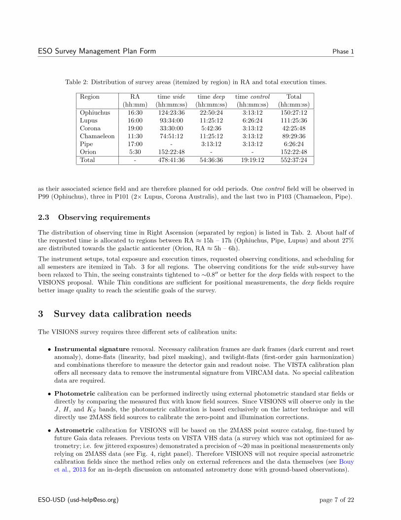
Table 2: Distribution of survey areas (itemized by region) in RA and total execution times.

Region RA time wide time deep time control Total(hh:mm) (hh:mm:ss) (hh:mm:ss) (hh:mm:ss) (hh:mm:ss)

Ophiuchus 16:30 124:23:36 22:50:24 3:13:12 150:27:12Lupus 16:00 93:34:00 11:25:12 6:26:24 111:25:36Corona 19:00 33:30:00 5:42:36 3:13:12 42:25:48Chamaeleon 11:30 74:51:12 11:25:12 3:13:12 89:29:36Pipe 17:00 - 3:13:12 3:13:12 6:26:24Orion 5:30 152:22:48 - - 152:22:48Total - 478:41:36 54:36:36 19:19:12 552:37:24

as their associated science field and are therefore planned for odd periods. One control field will be observed inP99 (Ophiuchus), three in P101 (2× Lupus, Corona Australis), and the last two in P103 (Chamaeleon, Pipe).

2.3 Observing requirements

The distribution of observing time in Right Ascension (separated by region) is listed in Tab. 2. About half ofthe requested time is allocated to regions between RA ≈ 15h – 17h (Ophiuchus, Pipe, Lupus) and about 27%are distributed towards the galactic anticenter (Orion, RA ≈ 5h – 6h).

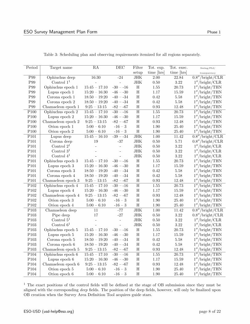
The instrument setups, total exposure and execution times, requested observing conditions, and scheduling forall semesters are itemized in Tab. 3 for all regions. The observing conditions for the wide sub-survey havebeen relaxed to Thin, the seeing constraints tightened to ∼0.8′′ or better for the deep fields with respect to theVISIONS proposal. While Thin conditions are sufficient for positional measurements, the deep fields requirebetter image quality to reach the scientific goals of the survey.

3 Survey data calibration needs

The VISIONS survey requires three different sets of calibration units:

• Instrumental signature removal. Necessary calibration frames are dark frames (dark current and resetanomaly), dome-flats (linearity, bad pixel masking), and twilight-flats (first-order gain harmonization)and combinations therefore to measure the detector gain and readout noise. The VISTA calibration planoffers all necessary data to remove the instrumental signature from VIRCAM data. No special calibrationdata are required.

• Photometric calibration can be performed indirectly using external photometric standard star fields ordirectly by comparing the measured flux with know field sources. Since VISIONS will observe only in theJ , H, and KS bands, the photometric calibration is based exclusively on the latter technique and willdirectly use 2MASS field sources to calibrate the zero-point and illumination corrections.

• Astrometric calibration for VISIONS will be based on the 2MASS point source catalog, fine-tuned byfuture Gaia data releases. Previous tests on VISTA VHS data (a survey which was not optimized for as-trometry; i.e. few jittered exposures) demonstrated a precision of ∼20 mas in positional measurements onlyrelying on 2MASS data (see Fig. 4, right panel). Therefore VISIONS will not require special astrometriccalibration fields since the method relies only on external references and the data themselves (see Bouyet al., 2013 for an in-depth discussion on automated astrometry done with ground-based observations).



Table 3: Scheduling plan and observing requirements itemized for all regions separately.

Period Target name RA DEC Filter Tot. exp. Tot. exec. Seeing/FLI/

setup time [hrs] time [hrs] transparency

P99 Ophiuchus deep 16:30 -24 JHK 2.00 22.84 0.8′′/bright/CLRP99 Control 11 - - JHK 0.50 3.22 1′′/bright/CLRP99 Ophiuchus epoch 1 15:45 – 17:10 -30 – -16 H 1.55 20.73 1′′/bright/THNP99 Lupus epoch 1 15:20 – 16:30 -46 – -30 H 1.17 15.59 1′′/bright/THNP99 Corona epoch 1 18:50 – 19:20 -40 – -34 H 0.42 5.58 1′′/bright/THNP99 Corona epoch 2 18:50 – 19:20 -40 – -34 H 0.42 5.58 1′′/bright/THNP99 Chamaeleon epoch 1 9:25 – 13:15 -82 – -67 H 0.93 12.48 1′′/bright/THNP100 Ophiuchus epoch 2 15:45 – 17:10 -30 – -16 H 1.55 20.73 1′′/bright/THNP100 Lupus epoch 2 15:20 – 16:30 -46 – -30 H 1.17 15.59 1′′/bright/THNP100 Chamaeleon epoch 2 9:25 – 13:15 -82 – -67 H 0.93 12.48 1′′/bright/THNP100 Orion epoch 1 5:00 – 6:10 -16 – 3 H 1.90 25.40 1′′/bright/THNP100 Orion epoch 2 5:00 – 6:10 -16 – 3 H 1.90 25.40 1′′/bright/THNP101 Lupus deep 15:45 – 16:10 -39 – -34 JHK 1.00 11.42 0.8′′/bright/CLRP101 Corona deep 19 -37 JHK 0.50 5.71 0.8′′/bright/CLRP101 Control 21 - - JHK 0.50 3.22 1′′/bright/CLRP101 Control 31 - - JHK 0.50 3.22 1′′/bright/CLRP101 Control 41 - - JHK 0.50 3.22 1′′/bright/CLRP101 Ophiuchus epoch 3 15:45 – 17:10 -30 – -16 H 1.55 20.73 1′′/bright/THNP101 Lupus epoch 3 15:20 – 16:30 -46 – -30 H 1.17 15.59 1′′/bright/THNP101 Corona epoch 3 18:50 – 19:20 -40 – -34 H 0.42 5.58 1′′/bright/THNP101 Corona epoch 4 18:50 – 19:20 -40 – -34 H 0.42 5.58 1′′/bright/THNP101 Chamaeleon epoch 3 9:25 – 13:15 -82 – -67 H 0.93 12.48 1′′/bright/THNP102 Ophiuchus epoch 4 15:45 – 17:10 -30 – -16 H 1.55 20.73 1′′/bright/THNP102 Lupus epoch 4 15:20 – 16:30 -46 – -30 H 1.17 15.59 1′′/bright/THNP102 Chamaeleon epoch 4 9:25 – 13:15 -82 – -67 H 0.93 12.48 1′′/bright/THNP102 Orion epoch 3 5:00 – 6:10 -16 – 3 H 1.90 25.40 1′′/bright/THNP102 Orion epoch 4 5:00 – 6:10 -16 – 3 H 1.90 25.40 1′′/bright/THNP103 Chamaeleon deep 11 -77 JHK 1.00 11.42 0.8′′/bright/CLRP103 Pipe deep 17 -27 JHK 0.50 3.22 0.8′′/bright/CLRP103 Control 51 - - JHK 0.50 3.22 1′′/bright/CLRP103 Control 61 - - JHK 0.50 3.22 1′′/bright/CLRP103 Ophiuchus epoch 5 15:45 – 17:10 -30 – -16 H 1.55 20.73 1′′/bright/THNP103 Lupus epoch 5 15:20 – 16:30 -46 – -30 H 1.17 15.59 1′′/bright/THNP103 Corona epoch 5 18:50 – 19:20 -40 – -34 H 0.42 5.58 1′′/bright/THNP103 Corona epoch 6 18:50 – 19:20 -40 – -34 H 0.42 5.58 1′′/bright/THNP103 Chamaeleon epoch 5 9:25 – 13:15 -82 – -67 H 0.93 12.48 1′′/bright/THNP104 Ophiuchus epoch 6 15:45 – 17:10 -30 – -16 H 1.55 20.73 1′′/bright/THNP104 Lupus epoch 6 15:20 – 16:30 -46 – -30 H 1.17 15.59 1′′/bright/THNP104 Chamaeleon epoch 6 9:25 – 13:15 -82 – -67 H 0.93 12.48 1′′/bright/THNP104 Orion epoch 5 5:00 – 6:10 -16 – 3 H 1.90 25.40 1′′/bright/THNP104 Orion epoch 6 5:00 – 6:10 -16 – 3 H 1.90 25.40 1′′/bright/THN

1 The exact positions of the control fields will be defined at the stage of OB submission since they must bealigned with the corresponding deep fields. The position of the deep fields, however, will only be finalized uponOB creation when the Survey Area Definition Tool acquires guide stars.



30 20 10 0 10 20 30∆X (arcmin)

40

30

20

10

0

10

20

30

40

∆Y (

arc

min

)

Our reduction

3020100102030∆X (arcmin)

CASU reduction

0.72 0.76 0.80 0.84 0.88 0.92 0.96 1.00PSF FWHM (arcsec)

3020100102030∆X (arcmin)

40

30

20

10

0

10

20

30

40

∆Y (

arc

min

)

Resolution gain

16.8 17.6 18.4 19.2 20.0 20.8 21.6 22.4Difference (%)

Figure 2: FWHM maps for both the Astropype reduction and the standard CASU pipeline of a tile in H band.Clearly a significant gain in image quality is achieved in our reduction. This figure was adopted from Meingastet al. (2016).

4 Data reduction process

The Meingast et al. (2016) VISTA survey of the Orion A molecular cloud demonstrated that the standardpipeline for VISTA data, operated by CASU, is not optimal for projects which aim for the highest imagequality and unbiased photometry. Two major drawbacks in the CASU processing method make an independentdata calibration necessary for the VISIONS project:

• To optimally co-add all reduced paw prints, each input image needs to be resampled onto a commonreference frame. The CASU pipeline uses a radial distortion model together with fast bilinear interpolationto remap the images for the final tiling step. Bilinear interpolation, however, has several drawbacks. Apartfrom significant dispersions in the measured fluxes, it additionally “smudges” the images, leading to loweroutput resolution (see Bertin, 2010 for details and examples).

• For the zero-point calculation of each observed field the CASU pipeline applies a galactic extinctioncorrection to all photometric measurements based on data from Schlegel et al. (1998) and Bonifacio et al.(2000). This will add systematic offsets with respect to photometric data for which no such correctionwas applied. For studies concerned with the intrinsic color of stars (e.g. extinction mapping), however, itis critical not to be biased in any way by such systematic offsets.

Meingast et al. (2016) implemented a completely independent data reduction environment, which (a) usessophisticated high-order resampling kernels and (b) directly calibrates the photometry towards the 2MASSsystem without biasing the results with galactic extinction corrections. Figure 2 shows a FWHM map for onobserved tile of the Orion A survey in H band for both the CASU and the improved reduction, as well as thecorresponding gain in resolution.

The optimized processing typically achieves 20% higher resolution compared to the standard CASU pipeline,i.e. a 20% smaller FWHM. In addition, one can observe a dependency of the resolution gain with observingconditions. While only a gain of 10-15% is reached for seeing conditions > 1 arcsec, up to almost 30% can be



gained for excellent conditions (∼ 0.6 arcsec). Moreover, the improved reduction recovers the image quality ofthe pawprint level for the combined tiles which is not the case for the CASU reduction.

4.1 Astropype Reduction Cascade

For VISIONS the Meingast et al. (2016) data reduction environment and all individual modules have beenaggregated into the stand-alone software package Astropype. The software was developed at the University ofVienna and is entirely written in Python. Astropype features fully automatic data processing optimized forVISTA, but it’s basic processing modules are in principle applicable to any other imaging data (Astropype wassuccessfully tested with VST and HAWK-I data products). For photometric and astrometric calibration andPSF analysis the pipeline environment relies on external software packages for which Python wrappers weredeveloped. Figure 3 shows a schematic overview of the principle data flow in the Astropype environment. Belowwe will only give a concise overview of the key features of the major data reduction steps. Details on eachindividual module are given in Meingast et al. (2016).

1. Completely self-contained master-calibration unit. All necessary calibration data are automatically gen-erated based on the time stamps in the FITS headers. Astropype is specifically tuned to generate mas-ter calibration units from the data collection as defined in the VISTA calibration plan. This includesbad-pixel-masks, master-darks, master-flatfields, weight-maps (also referred to as confidence maps), andlinearity tables. In addition Astropype generates astrometric and photometric reference catalogs, as wellas sky-frames for background modeling.

2. The master-calibration units are subsequently used to process the raw science data to remove the basicinstrumental signature and the sky background from the VIRCAM images.

3. External references (2MASS and Gaia catalogs) are then used to simultaneously perform photometricand astrometric calibration via Scamp (Bertin, 2006). Following the initial photometric calibration anillumination correction is calculated directly from the external reference data. This process generatesmodified external calibration headers which contain astrometric information, as well as the necessaryflux-scaling parameters for gain-harmonization, illumination correction, and photometric standardization.

4. All processed data are subsequently scaled and resampled onto a common reference frame and zero-pointwith SWarp (Bertin, 2010) using high-order resampling kernels.

5. From these resampled frames Astropype constructs calibrated pawprints and tiles and generates severalquality control and global calibration units (e.g. aperture corrections). These pawprints and tiles are partof the VISIONS data products.

6. The constructed pawprints and tiles are then processed with SExtractor (Bertin and Arnouts, 1996) andPSFEx (Bertin, 2011) to generate source catalogs.

7. These raw source catalogs are then subject to further processing where e.g. aperture corrections andmachine-learning-based morphological classification schemes are applied (see Fig. 9 in Meingast et al.,2016). In addition sources are cross-correlated with various quality control parameters and calibrationunits (completeness, local image quality, total effective exposure time, etc.)

Once data calibration for VISIONS commences and the Astropype code has been frozen, the software will bemade publicly available on Github.

4.2 Benchmark

To estimate the total time required to process a typical night, we downloaded and processed a random night(2015-01-16) from the ESO Public Archives. A total of 775 files, including calibrations, ESO QC and scientific



Master calibrationBPM

Dark

Flat

Sky

Linearity

Weight

Phot. ref.

Astr. ref.

VISTA calibration plan 2MASS/Gaia

Raw science

Linearity

Dark

Flat

Sky

QC

QC

External calibration header

Astr. ref. Phot. ref.

Resampled science

SWarp

Pawprints Tiles

QC

Catalog Catalog

QC

SExtractor

Scamp

PSFEx

Processed science

Weight

SExtractor

PSFEx

SExtractor

PSFEx

Multi-epoch

Variables

Band-merged

Figure 3: Schematic view of the basic Astropype processing steps. Input data is highlighted in red, calibrationsteps in yellow, quality control in blue, intermediate products in white, external software in gray, and deliverablesin green.



images, were retrieved, totalizing 48GB of data. Table4 gives an overview of the execution times of the mainreduction steps.

Table 4: Execution time for the various processing stepsDownload from archive 45 minDecompressing 20 minSplitting MEF 60 minProcess Master Calibrations 1 minPre-Process Science Files 11 minAstrometric + Photometric Solution 55 minCo-addition 75 minFinal source extraction 10 min

Total: 4.5h

These benchmarks were obtained on a cluster made of 140 CPU with fast stripped hard drives and a 10GB/snetwork. This cluster will undergo a major upgrade in Nov. 2016 (see Section 5.1 below) and these dataprocessing times should be greatly reduced. The above estimate should therefore be regarded as a conservativelimit. It nevertheless demonstrates our capacity to download and process the observations on a nightly basis,which will be essential to provide a almost real-time feedback to the observatory.

5 Manpower and hardware capabilities devoted to data reductionand quality assessment

The VISIONS survey team will be structured into two major groups: the Survey Management Team (SMT)and the Survey Support Team (SST). While the former is responsible for the successful execution of the survey,the latter consists of multiple joint work groups which are specialized in specific tasks. The SMT will workcontinuously over the entire duration the survey, with monthly meetings, while the SST will work on particulartime blocks on specific tasks.

The survey activities will be coordinated and overseen by the SMT (Alves, Bouy, Meingast). The SMT isalso responsible for the survey preparation (e.g. OB submission) and the timely delivery of Phase 3 dataproducts (contact point, Meingast). They will also manage and distribute tasks (e.g. quality control, pipelineupgrades) to specific panels of the SST. Each panel will be chaired by a responsible, supported by other teammembers. From experience, many issues only become apparent when working directly with the generated data.Each member of our team has a personal scientific interest in these data, which will guarantee quick real-lifetests. The panels of the SST cover all major technical and scientific aspects of VISIONS: Survey executionand progress; pipeline/photometry/astrometry; data quality; stellar clusters; young stellar objects; positionsand proper motions; dust properties. Each member is assigned to multiple support teams according to theirspecialization and scientific interests. A description of the detailed responsibilities of the members of theVISIONS survey team, their affiliation, and FTE commitment to the project is given in Tab. 5

5.1 Hardware

Processing and storing the large amount of data produced by VISIONS will require powerful high-performancecomputing facilities. We estimate that 500TB of disk space will be required to store and process the entiredataset produced over the duration of VISIONS. High throughput and parallelization will be essential for anefficient and timely processing of the continuous data flow, allowing a rapid quality check of the data andresponsive feedback to the observatory.

We will have access to several computing facilities, all already funded:



Table 5: Allocation of resources within the VISIONS survey team.

Name Function Affiliation Country FTE

Survey Management TeamJ. Alves PI U Vienna A 0.2H. Bouy Co-PI U Bordeaux F 0.2S. Meingast Co-PI (contact point) U Vienna A 0.8

Survey Support TeamJ. Ascenso Young clusters, dust properties FEUP P 0.1A. Bayo SED modeling and APOGEE U Valparaiso RCH 0.1E. Bertin Pipeline and web interface IAP F 0.1A. Brown Interface with Gaia Leiden U NL 0.05J. de Bruijne Interface with Gaia ESA ESA 0.05J. Forbrich Radio astrometry, dust properties U Vienna A 0.1J. Großchedl Observation preparation, YSOs U Vienna A 0.1A. Hacar Cluster formation Leiden U NL 0.2B. Hasenberger Observation preparation, CMF/IMF U Vienna A 0.1J. Kainulainen Density mapping, structure analysis MPIA D 0.2J. Kauffmann Interface with SDSS MPfR D 0.1R. Kohler Binaries, jets proper motions U Vienna A 0.1K. Kubiak Observation preparation, dispersed population U Vienna A 0.1K. Leschinski Observation preparation, streams U Vienna A 0.1M. Lombardi Extinction mapping U Milan I 0.1D. Mardones Jets and outflows, obs. preparation U Chile RCH 0.1A. Moitinho Young optical population U Lisboa P 0.1K. Pena Ramırez Interface with VVV, IMF U Cat. Chile RCH 0.1M. Petr-Gotzens Observation preparation, binaries, IMF ESO ESO 0.1T. Prusti Interface with Gaia ESA ESA 0.05R. Ramlau PSF reconstruction, image quality U Linz A 0.1T. Robitaille Consultant (Hyperion, astropy) UK 0.1P. Teixeira Observation preparation, binaries U Vienna A 0.1E. Zari Interface with Gaia Leiden U NL 0.1W. Zeilinger Observation preparation, galaxy clusters U Vienna A 0.15

Planned positionsPostdoc Cloud structure analysis MPIA D 0.6Postdoc Data reduction U Bordeaux F 0.3PhD student 3D modeling U Vienna A 0.8



• A HPC cluster located at the University of Bordeaux and owned entirely by H. Bouy. It will consist of 448modern Intel CPU and 10 NVIDIA Pascal GPU, 1TB of RAM and will include 1.5PB of high-throughputenterprise-grade redundant (RAID) disk space, and a 40 Gigabyte/s Omnipath Network. This cluster isfully funded and is under design at DELL and will be delivered by the end of 2016.

• Dedicated high-performance workstations at the University of Vienna with high-throughput enterprise-grade redundant (RAID) disk space. A new set of workstations will be acquired in 2018 to complementthe HPC cluster and small workstations and laptop.

• Personal computers for administration, reports, OB preparation, etc.

This hardware is offering a CPU and RAM overcapacity of at least 5 and a storage overcapacity of at least 3for the VISIONS processing pipeline and expected dataflow. It therefore ensures that we will be able to dealwith the data and eventual variations of data flow rates and reprocessing requirements on a nightly basis, asdescribed in Section 4.2. All raw and processed files will be stored using lossless Rice tile compression to savea factor of 4 in storage requirements.

In addition to the computing facilities mentioned above, we will set up our own public cloud server and archiveto share internally and externally all the raw and processed images and catalogues. A dedicated server willhost a visualization interface based on the VisiOmatic software where users will be able to access, browse andexplore the processed images and catalogues, enhancing and increasing the impact of ESO data. Finally, modernweb-based collaborative tools, including a project management software, Wiki and WebRTC communicationsoftware, will give us full control of task and time management, team collaboration and reporting.

6 Data quality assessment process

The main resource for quality assessment for all data products will be dedicated quality control units generatedby the pipeline infrastructure. These are produced at various stages in the data flow (compare Fig. 3). Examplesof these units created by Astropype are shown in Fig. 2 (PSF FWHM map of a stacked VISTA tile), Fig. 4(aperture correction and positional residuals during astrometric calibration), and Fig. 5 (detector non-linearityas measured from a VISTA dome-flat sequence). Other units generated by Astropype include, bad-pixel fraction,dark current, read-noise, gain variation, sky background variation, zero-point verification (fitting uncertainty,residual 1D and 2D variations after photometric flux scaling). The processed data will also include a suite ofquality control parameters stored in the FITS headers including Phase 3 compliant information (e.g. limitingmagnitude, saturation limit, spatial resolution, source ellipticity).

In addition to the survey team members responsible for quality assessment who will continuously monitor thesequality control units, Astropype will also prompt warnings in case predefined upper and lower boundaries forthe quality parameters are exceeded (e.g. bad pixel fraction, fitting uncertainties, etc.) upon which the surveyteam will investigate possible issues.

Since CASU already operates a stable pipeline environment for VISTA, the quality control parameters derivedby Astropype and the general data products (e.g. processed pawprints) will also be compared to the standardVISTA pipeline reduction to identify potential systematic errors.

7 External Data products and Phase 3 compliance

The VISIONS data products will be delivered according to the ESO Phase 3 policies. All science productswill initially be made available via the ESO Phase 3 ecosystem and will comply to the given standards (e.g.metadata FITS header QC keywords). Any subsequent publication via e.g. CDS will acknowledge ESO as dataorigin. The following data products will be made available:



Figure 4: Left: Aperture correction quality control unit generated by Astropype for the KS control field ofMeingast et al. (2016). Right: 2D internal astrometric residuals obtained for a test-sample of 1600 KS VHSVISTA images. The gray curve represents the integrated distribution for SNR> 100 sources, and the greencurve the integrated distribution for SNR=10. They have a 1-σ dispersion of ∼ 20mas.

• Processed pawprints with removed instrumental signature including photometric and astrometric (com-pliant with the WCS standard) calibration, with Phase 3 compatible FITS headers. All processing stepswill also be documented in the headers.

• Stacked tiles constructed from the processed pawprints (also Phase 3 compliant with appropriate headers).

• Weight (confidence) maps for both the processed pawprints as well as the stacked tiles.

• Quality control database including maps tracing background noise, seeing, PSF shape, exposure time,frame coverage, effective observing time, and completeness estimates (see Meingast et al., 2016 for exam-ples).

• Derived source catalogs for both pawprints and stacked tiles, including positions, multi-aperture photom-etry, and morphological classification.

• Homogeneous band-merged catalogues directly constructed from the VISIONS data (deep and controlsurvey) or merged with VHS data (wide survey).

8 Delivery timeline of data products to the ESO archive

Simultaneously with the start of the VISIONS observations in P99 (April 2017), the team members in charge ofdata reduction and quality assessment will continuously monitor the survey progress. The survey team expectsa test phase of 6 months for final pipeline implementation, initial data validation and quality assurance. Assoon as a stable setup is achieved, data reduction will commence and will continue parallel to the observations.

The survey team plans in total three data releases:

• October 2018, DR1: 18 months after the start of the public survey operations in April 2017, the initialrelease of VISIONS will include all available data products of the deep and control observations that were



8000

16000

24000

32000

40000

AD

U

NL10000 = 0.42%

Det.ID: 1

NL10000 = 1.44%

Det.ID: 2

NL10000 = 1.26%

Det.ID: 3

NL10000 = 0.14%

Det.ID: 4

8000

16000

24000

32000

40000

AD

U

NL10000 = 2.82%

Det.ID: 5

NL10000 = 0.49%

Det.ID: 6

NL10000 = 0.4%

Det.ID: 7

NL10000 = 1.0%

Det.ID: 8

8000

16000

24000

32000

40000

AD

U

NL10000 = 1.06%

Det.ID: 9

NL10000 = 0.53%

Det.ID: 10

NL10000 = 1.51%

Det.ID: 11

NL10000 = 0.42%

Det.ID: 12

10 20 30 40DIT (s)

8000

16000

24000

32000

40000

AD

U

NL10000 = 6.15%

Det.ID: 13

10 20 30 40DIT (s)

NL10000 = 0.86%

Det.ID: 14

10 20 30 40DIT (s)

NL10000 = 0.24%

Det.ID: 15

10 20 30 40DIT (s)

NL10000 = 1.39%

Det.ID: 16

Figure 5: QC unit generated by Astropype to measure non-linearity of the VIRCAM detectors for a randomlyselected dome-flat sequence from the VISTA calibration plan.



observed by April 2018. This includes all processed and calibrated pawprints and tiles, the completeband-merged source catalogs as well as various advanced quality control units.

• October 2019, DR2: Release of photometry for the wide survey. As in DR1 this release consists ofcalibrated pawprints, tiles, and source catalogs. DR2 will also be complemented by all additional deepand control fields which have been observed by April 2019.

• October 2020, DR3: Final release of the wide survey data products. Building on DR2, this releasewill include multi-epoch photometry (6 epoch wide survey) and positions of all detected sources. Alsoremaining deep and control sub-survey data products will also be made available. In addition we willprovide the final mosaics via the VisiOmatic web interface (Bertin et al., 2015). A sample illustratingsome of the numerous capabilities can be seen on the following webpage: http://visiomatic.iap.fr/pleiades/

References

Bertin, E. (2006). Automatic Astrometric and Photometric Calibration with SCAMP. In Gabriel, C., Arviset,C., Ponz, D., and Enrique, S., editors, Astronomical Data Analysis Software and Systems XV, volume 351 ofAstronomical Society of the Pacific Conference Series, page 112.

Bertin, E. (2010). SWarp: Resampling and Co-adding FITS Images Together. Astrophysics Source CodeLibrary.

Bertin, E. (2011). Automated Morphometry with SExtractor and PSFEx. In Evans, I. N., Accomazzi, A.,Mink, D. J., and Rots, A. H., editors, Astronomical Data Analysis Software and Systems XX, volume 442 ofAstronomical Society of the Pacific Conference Series, page 435.

Bertin, E. and Arnouts, S. (1996). SExtractor: Software for source extraction. Astronomy and AstrophysicsSupplement, 117:393–404.

Bertin, E., Pillay, R., and Marmo, C. (2015). Web-based visualization of very large scientific astronomy imagery.Astronomy and Computing, 10:43–53.

Bonifacio, P., Monai, S., and Beers, T. C. (2000). A Search for Stars of Very Low Metal Abundance. V.Photoelectric UBV Photometry of Metal-weak Candidates from the Northern HK Survey. AstronomicalJournal, 120:2065–2081.

Bonnarel, F., Fernique, P., Bienayme, O., Egret, D., Genova, F., Louys, M., Ochsenbein, F., Wenger, M., andBartlett, J. G. (2000). The ALADIN interactive sky atlas. A reference tool for identification of astronomicalsources. Astronomy and Astrophysics Supplement, 143:33–40.

Bouy, H., Bertin, E., Moraux, E., Cuillandre, J.-C., Bouvier, J., Barrado, D., Solano, E., and Bayo, A. (2013).Dynamical analysis of nearby clusters. Automated astrometry from the ground: precision proper motionsover a wide field. Astronomy & Astrophysics, 554:A101.

Meingast, S., Alves, J., Mardones, D., Teixeira, P., Lombardi, M., Großschedl, J., Ascenso, J., Bouy, H.,Forbrich, J., Goodman, A., Hacar, A., Hasenberger, B., Kainulainen, J., Kubiak, K., Lada, C., Lada, E.,Moitinho, A., Petr-Gotzens, M., Rodrigues, L., and Roman-Zuniga, C. G. (2016). VISION - Vienna surveyin Orion I. VISTA Orion A Survey. Astronomy & Astrophysics, 587:A153.

Schlegel, D. J., Finkbeiner, D. P., and Davis, M. (1998). Maps of Dust Infrared Emission for Use in Estimation ofReddening and Cosmic Microwave Background Radiation Foregrounds. The Astrophysical Journal, 500:525–553.


http://visiomatic.iap.fr/pleiades/


Skrutskie, M. F., Cutri, R. M., Stiening, R., Weinberg, M. D., Schneider, S., Carpenter, J. M., Beichman, C.,Capps, R., Chester, T., Elias, J., Huchra, J., Liebert, J., Lonsdale, C., Monet, D. G., Price, S., Seitzer, P.,Jarrett, T., Kirkpatrick, J. D., Gizis, J. E., Howard, E., Evans, T., Fowler, J., Fullmer, L., Hurt, R., Light,R., Kopan, E. L., Marsh, K. A., McCallon, H. L., Tam, R., Van Dyk, S., and Wheelock, S. (2006). The TwoMicron All Sky Survey (2MASS). The Astronomical Journal, 131:1163–1183.

Spezzi, L., Petr-Gotzens, M. G., Alcala, J. M., Jørgensen, J. K., Stanke, T., Lombardi, M., and Alves, J. F.(2015). The VISTA Orion mini-survey: star formation in the Lynds 1630 North cloud. Astronomy &Astrophysics, 581:A140.



Appendix A: Response to EST/ASG/instrument scientist Report

1. Phase 1: the team is requesting 75 hrs with more stringent observing conditions with respect to thesubmitted proposal. The request of 0.8 for fields at airmass 1.6 -1.7 (Chamaeleon SFR) is particularlydifficult to achieve. The team is asked to modify this request in the revised SMP by relaxing the observingconstraints. For scheduling purposes, the more stringent conditions may be accepted for no more than 20hrs per semester.

The deep and control survey strategies have been revised to allow for more efficient schedul-ing. To this end we relaxed the observing constraints for the control fields to 1′′ seeing(but keeping CLR conditions) and instead of scheduling all deep and control blocks in P99,each odd semester now includes a set of these observations. For P99 we schedule Ophiuchus(execution time: 22h 50m 24s) and one control field, for P101 Lupus (11h 25m 12s), Corona(5h 42m 36s), and three control fields, and for P103 we will observe Chamaeleon (11h 25m12s), the Pipe (3h 13m 12s), and the remaining two control fields. In addition we adjustedthe delivery timeline of the survey science products accordingly.

The VISIONS team is also aware that 0.8′′ for Chamaeleon are difficult to achieve. However,previous surveys have shown that such conditions can be met at similar altitudes (e.g.LMC/SMC). The Chamaeleon field is visible in both observing semesters where the deepfield is currently scheduled for P103 and requires an execution time of 11.4h. If the criteriaare not met within this time frame, it is possible to relax the constraints for subsequentobservations in P104.

2. Phase 1: Please add in Sec. 2.1.2 the information that the OB strategy for the deep survey OBs includessky offset fields, which leads to longer OB execution times than for the otherwise identical control fieldsurvey OBs.

Section 2.1.2 has been rewritten to consider all changes with respect to the deep survey andnow also describes the sky offset strategy in detail.

3. Phase 2: OBs of 1hr:57 min are very long and the PI should be aware of the QC policy that if the conditionsdegrade after the first hour of execution, in violation of the constraints, the OB would be continued andwill not be repeated. This means that such a long OB execution will not guarantee homogeneous imagequality. A split into two OBs might result in more homogeneous quality and also ease the scheduling.

The OBs for the deep fields including sky offsets have been split into two separate blocks,each including three (of the in total six) jittered positions. Instead of 1h 57m 42s runtimes(for H and KS), the split OBs now are executed in one hour each. The J band deep OBsnow take 2× 51m instead of 1h 39m 42s. Individual deep field regions are still scheduled tobe observed in the same semester. The longest OB execution times now are 1h 10m 24s forthe control and deep (Pipe) observations without sky offsets. Executing the two split OBsleads to a longer observing duration compared to using only one long OB. However, sincewe also removed the sky offsets for the Pipe Nebula the deep survey now requires less time(54h 36m 36s instead of 55h 51m in the previous survey plan). Due to the revised strategythe total requested time has changed to 552h 37m 24s.

4. Phase 2: time sequences of concatenation of OBs are NOT possible. Please revise the observing strategywhereby concatenation of OBs are defined with absolute time windows.

We have adjusted the observing strategy for the wide fields in such a way that absolutetime intervals will be defined for a set of four concatenated OBs. Time-link containers willtherefore not be required for scheduling. All wide OBs will be given certain absolute timeintervals in which they should be observed (6-8 weeks). The next epoch of the same field willthen be defined so that there is minimum break of two months. This is especially importantfor wide fields which have two scheduled epochs in one semester (Corona Australis andOrion).



5. Phase 2: For OBs with short exposures (NDIT x DIT < 31 secs) one can get high ellipticity. It helps toset AG=T for the first pawprint.

We acknowledge this very helpful hint, will follow the recommendations, and have added astatement to Sect. 2.1.1.

6. Quality control: QC parameters referring to science data products must be included in the FITS headerof the respective file. Example: PSF FWHM. The team may add its own parameters to complement theset of SDPS keywords. See P.12 below for Phase 3 standard validation.

The survey team is aware of these requirements. All necessary QC parameters will begenerated by our pipeline and will be added to the phase 3 products. A short statementhas been added to Sect. 7.

7. FTE/resource allocation: it is worrisome that the PI allocated only 0.2 FTE yearly to the survey. Manyallocations to team members at the level of 0.1 FTE, which is not effective.

We understand the concern but we see the FTE contributions as mean contributions tothe project. A typical 0.1 FTE contribution should not be seen as 4h per week but as aspecific intense period of work for a particular task that, on average, over the duration ofthe survey, will take 0.1 FTE per year. In contrast, the 1.2 FTE for the SMT should be seenas a continuous contribution. We changed the contribution from a post-doc in Table 5 from0.2 to 0.3 FTE. Although this might not alleviate all concerns, we are currently procuringfunds for a PhD position for which we already have have part of the money. We plan to use100% of this position to the project, although we do not list it yet on Table 5.

8. FTE/resource allocation: Table 4 should indicate the team member responsible for the OPC report andthe assignee of the Phase3 survey manager role, i.e. who is responsible for data release planning, validationand documentation (data release description).

The SMT as a whole (Alves, Bouy, Meingast) is the direct responsible for the OPC reportand the assignee of the Phase 3 survey manager role, and will work tightly, via monthlytelecons, to keep the survey obligations on time. If a single contact person is necessary forthese tasks, this should be Co-PI Stefan Meingast.

9. FTE/resource allocation: it is noted that the hardware for data processing becomes available to the teamat the end of 2017/2018, hence it is not available (installed, commissioned and tested in operation) at thestart of the survey. This is a concern as it is likely to propagate in a backlog of data to be processed, andgenerate substantial delays for the data releases and science exploitation. The team is asked to describethe mitigating strategies to be set in place to secure an earlier the delivery of the hardware and carry outan efficient commissioning.

It was a mistake. The HPC cluster is fully funded and is being designed at the momentwith the DELL team. We expect a delivery by the end of 2016, 6 months before the start ofobservations. Its characteristics have been updated, and it represents a large overcapacitywith respect to the expected requirements to process the survey.

10. FTE/resource allocation: the team is asked to provide an estimate of how long it takes to process onenight of VIRCAM data, in order to assess the time required to process the entire backlog of raw data,caused by any delays in the delivery of the hardware or commissioning of the pipelines.

A new section 4.2 has been added. We find that it takes about 4.5h to process an typicalnight with our current HPC cluster. This figure should drop by at least 30% with the newfacility expected for the end of the year.

11. Phase 3: the team is asked to carry out a Phase 3 format and provenance verification of their products asto check the compliancy of the metadata information and data format with the phase 3 standard. Theiralready reduced and published data for VISION (Meingast et al. 2016) could be used as a test data set.



We also acknowledge this additional helpful advice and the survey team will carry out aPhase 3 verification with the VISION data before the start of the VISIONS operations inApril 2017. We expect that this step will minimize the potential issues when preparing thenew survey data for the subsequent Phase 3 release.

12. Phase 3: Master calibration frames are generated by ESO on a regular basis and made available to thecommunity via the ESO archive. The scope of Phase 3 delivery are science data-products only (as definedin ESO/SDPS doc. and the published amendments)

We have removed the master-calibration units (darks, flats, linearity) from the providedexternal data products in Phase 3 (see Sect. 7). However, the team still plans to provideadvanced calibration units to the community including data from our quality control setup(image quality maps, completeness, etc.).

13. Phase 3: The science data products must be submitted via Phase 3, to be compliant with ESO PSpolicies, despite possible redistribution through other channels (pls. acknowledge ESO as data origin; andfollow requirements for third parties distributing ESO data http://archive.eso.org/cms/eso-data-access-policy.html )

The VISIONS team is aware of these policies and the initial release of all science dataproducts will be made via the ESO phase 3 infrastructure. Subsequent publications (e.g.via CDS) will acknowledge ESO as data origin.

13a. One point still open: Not clear whether they deliver light curves from multi epoch observations: in Section7 they state “Homogeneous band-merged catalogues directly constructed from the VISIONS data, but notclear statement about multi-epoch photometry data. These deliverables are then listed in Section 8 (tobe included in DR3), but not included in the detailed list of products in Section 7. Please clarify in therevised SMP to be published on the ESO web site.

We will provide multi-epoch photometry for all wide fields in one final single catalog. Everyobject will have, when detected, six flux measurements. We removed the statement onvariability flags from section 8.



Appendix B: Changelog

1. Following the request to modify the deep survey strategy, we now distribute the deep and control sub-surveys over multiple periods. This was preferred over relaxing the observing constraints to 1′′ seeing.

2. The changed schedule for the deep and control sub-surveys made it necessary to adapt the delivery timelineof VISIONS data products. Instead of releasing the deep and control data with DR1, these data are nowalso distributed over the three planned releases.

3. For easier scheduling, the observing conditions for the control fields have been relaxed to 1′′.

4. The long deep sub-survey OBs including sky offsets have been split into two separate OBs with theconsequence that the total execution time for these deep OBs increased. However, we have removed thesky offset observations for the Pipe Nebula deep field since we do not expect large amounts of extendedemission in this region. In total the duration of the deep survey decreased from 55h 51m to 54h 36m 36s.

5. As a consequence of the adjustment of the deep survey, the total requested time for VISIONS now amounts552h 37m 24s (instead of 553h 51m 48s).

6. We have adjusted the observing strategy of the wide fields so that no time-links between concatenationsare required (which is not possible). Instead we will create OBs with absolute time intervals for each widesub-survey.

7. We have rephrased various statements concerning FTE contributions from the survey team. In particularwe highlight, that the relatively small contributions (0.1 FTE) are considered specific tasks at particularstages of the survey (e.g. OB creation) and are not meant as a continuous contribution. In contrast, theSurvey Management Team will work closely together over the entire duration of VISIONS.

8. We corrected errors in the description of the hardware deployment and added a section including aprocessing benchmark for a typical VISTA/VIRCAM night.

9. We removed master-calibration units (bad pixel masks, master-darks, master-flats, non-linearity tables)from the Phase 3 deliverables since these are also being made available by ESO via the ESO archive.

10. We acknowledge the very helpful tips of the ESO Survey Team, the VISTA/VIRCAM instrument scientists,and the Archive Science group and have taken their suggestions into account. This includes the setup ofthe active optics, the various suggestions related to Phase 3, and the notes on ESO public survey policies.


1 visions - vista star formation atlas - eso · 1 visions - vista star formation atlas pi: j....

Documents