1

Wright State UniversityBiomedical, Industrial & Human Factors Eng.

Search Theory Optimization:Agent Models and the Bay of Biscay

Raymond HillResearch sponsored in part by:

2

Purpose

Update with project results of DMSO/AFRL sponsored research conducted via AFIT Operational Sciences Department WSU BIE Department

Talk some about agent models Cover the optimization results Cover the game theory results Cover the search theory results Future directions (I hope)

3

Quick Background on Project

Lots of interest in agent models Project Albert work Brawler modeling work Next Generation Mission Model

Other agent model work as well Adaptive interface agents Intelligent software agents Internet agents

Challenge is how to bring agent models into the higher level models?

4

Why A Higher Level Modeling?

Need to better capture command and control effects

Need to capture “intangibles” Need to model learning based on battlefield

information Need better representation of actual

information use versus perfect use Agents and agent models hold promise but

bring along many issues

5

Agent Modeling Challenges

Output analysis Particularly with more complex models and models that are

not necessarily replicable

Accurate human behavior modeling In particular, command behavior modeling

Level of fidelity in model Beyond that of bouncing dots found in the complex

adaptive systems work

Interaction of agents and legacy modeling approaches Brawler extensions into theater and campaign level

modeling

6

Agent Modeling Challenges (cont).

Human interaction with the models The visual impact of interactions among the

agents “What if” analyses when human behavior is being

modeled Quantifiable aspects of generally qualitative types

of output Verification and Validation of the behaviors

embedded within the model

7

The Project

Needed a “use case” for agent models

Dr McCue’s book great example of operational analysis

Bay of Biscay scenario amenable to agent modeling Lots of information available

Formed an ideal basis for subsequent research

8

Efforts Completed

Capt Joe Price (masters thesis) Game theory focus

Capt Ron “Greg” Carl (masters thesis) Search theory focus Entering PhD this fall at Purdue

Subhashini Ganapathy Simulation optimization study PhD Candidate

Maj Lance Champagne, Ph.D. Dissertation completed March 2004

9

Snapshot of AFIT Model

10

Methodology - Game Portion

Allied search strategies When to search? Day versus night?

German U-boat surfacing strategies When to surface? Day versus night?

Two-person zero-sum game Players: Allied search aircraft and German U-boats Met rationality assumption

Non-perfect information Neither side knows the exact strategy the other uses

Objective is number of U-boat detections Allied goal: maximize German goal: minimize

Zero-sum game

11

Game Formulation

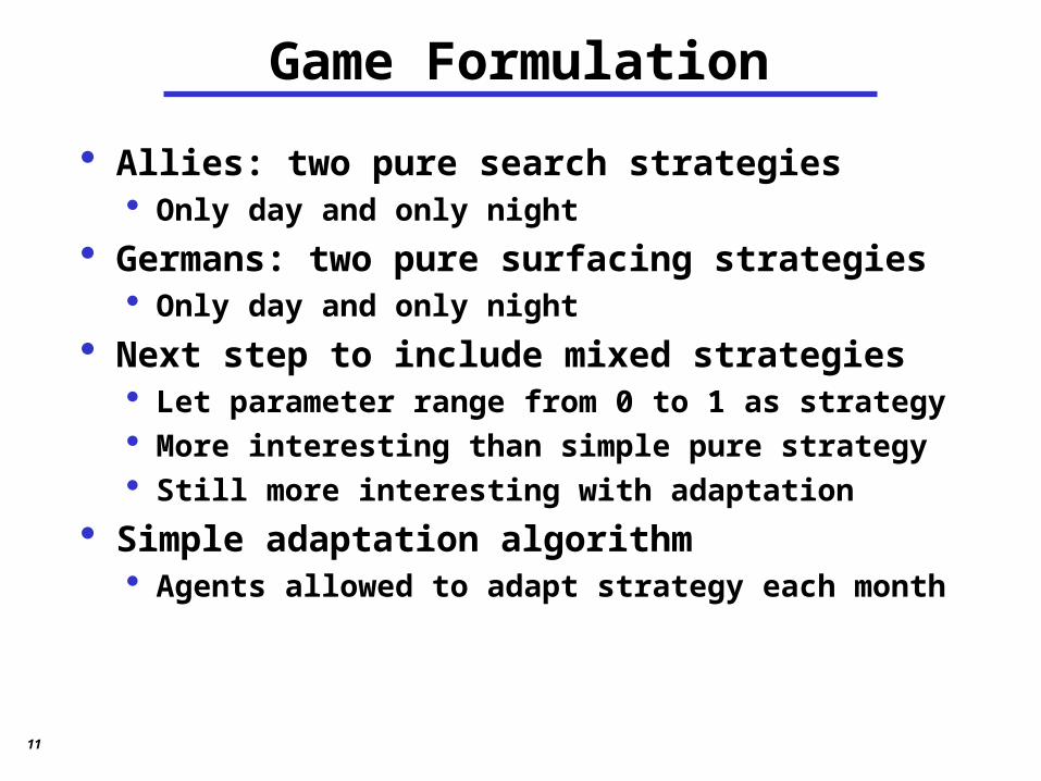
Allies: two pure search strategies Only day and only night

Germans: two pure surfacing strategies Only day and only night

Next step to include mixed strategies Let parameter range from 0 to 1 as strategy More interesting than simple pure strategy Still more interesting with adaptation

Simple adaptation algorithm Agents allowed to adapt strategy each month

12

Results – No Adaptation

Response Surface Methodology model Adjusted R2 = 0.947

1U

-Boa

t Day

Str

ateg

y0

U-Boat Detections

600

500

400

300

200

100

0

0 Aircraft Day Strategy 1

0

Aircraft Day Strategy

U-Boat Day Strategy

U-Boat Detections

Equilibrium Point, 0.7, 0.54

13

Adaptation Experiment

Design Point

Allied Search Strategy - Start

Allied Search Strategy - End

U-Boat Surfacing Strategy - Start

U-Boat Surfacing

Strategy - End

Average Number U-Boat

Detections1 (1, 0) (0.542, 0.458) (0, 1) (0.164, 0.836) 183.752 (1, 0) (0.625, 0.375) (1, 0) (0.327, 0.673) 180.453 (0.5, 0.5) (0.522, 0.478) (0.5, 0.5) (0.259, 0.741) 182.6

Both sides can adapt strategies (simple model) Three design points chosen: Adaptation occurs every month Investigate results 20 replications; 12-month warm-up; 12 months of

statistics collection (April 1943 – February 1944)

14

Adaptation ConvergenceTwo-Player Adaptation

Design Point 1

0

0.1

0.2

0.3

0.4

0.5

0.6

0.7

0.8

0.9

1

Start 1 2 3 4 5 6 7 8 9 10 11 12

Update (Months)

Da

y S

tra

teg

y

Aircraft Day Strategy U-Boat Day Strategy

Aircraft Starting Strategy: (1, 0)U-Boat Starting Strategy: (0, 1)

15

Adaptation ConvergenceTwo-Player Adaptation

Design Point 3

0

0.1

0.2

0.3

0.4

0.5

0.6

0.7

0.8

0.9

1

Start 1 2 3 4 5 6 7 8 9 10 11 12

Update (Months)

Da

y S

trat

egy

Aircraft Day Strategy U-Boat Day Strategy

Aircraft Starting Strategy: (0.5, 0.5)U-Boat Starting Strategy: (0.5, 0.5)

16

Methodology - Search Portion

Design data compiled according to hierarchy Historical fact Published studies Data derived from raw numbers Good judgment

MOE is number of U-boat sightings U-boat density constant between replications Aircraft flight hours same between replications Therefore, sightings = search efficiency

Two cases; search regions don’t overlap, do overlap

17

350

NM

2200 NM2

Non-overlapping Search Regions

18

100

NM

2100 NM2

Overlapping Search Regions

19

Aircraft Search Patterns

Barrier SearchParallel Line SearchCreeping Line SearchSector SearchSquare Search

20

Non-overlapping Search Regions

Means Comparison—All Pairs (20 Iterations)(Similar Letters Indicate Statistical Equivalence)

Search Pattern

Mean Sightings

Square A 106.9Creeping Line A B 98.3Barrier Patrol B 96.4Sector B 91.9Parallel B 91.7

21

Non-overlapping Search Regions

Means Comparison—All Pairs (30 Iterations)(Similar Letters Indicate Statistical Equivalence)

Search Pattern

Mean Sightings

Square A 105.9Creeping Line B 97.3Barrier Patrol B 91.4

22

Overlapping Search Regions

Means Comparison—All Pairs (30 Iterations)(Similar Letters Indicate Statistical Equivalence)

Search Pattern

Mean Sightings

Square A 122.1Parallel A 121.0Barrier Patrol A 118.0Sector A 115.6Creeping Line A 115.6

23

Simulation Optimization Portion

Simulation-based optimization is the process of finding the best input variable from all possibilities without explicitly examining each possibility

Often involves the use of some search heuristic “wrapped” around the simulation The simulation becomes the evaluation function The heuristic sends potential solutions to the

evaluation function The returned evaluations are then used to update

the search and eventually return a high-quality, possibly optimal solution

24

Graphic of Sim.-Based Opt.

Optimization Module(for the examples: Max Targets Found s.t. non-linear and stochastic variables)

Applies Generalized Reduced Gradient Method (search for alternatives along curves of the feasible region)

Simulation Module(emulates the system being studied by representing the entities & behavior)

25

The Entities, States and Events

Starting Point of Aircraft

• Refuel• Reloading of Ammunitions• Take-off point

Starting Point of Aircraft

• Refuel• Reloading of Ammunitions• Take-off point

Starting Point of U-Boats

• Refuel• Repair

Starting Point of U-Boats

• Refuel• Repair

Bay of Biscay

• U-Boats traveling under the sea• U-Boats traveling on the surface• Aircraft in search of U-Boats• Aircraft attacking U- Boats• Sunk U-Boats

Bay of Biscay

• U-Boats traveling under the sea• U-Boats traveling on the surface• Aircraft in search of U-Boats• Aircraft attacking U- Boats• Sunk U-Boats

U-boats in AtlanticU-boats in Atlantic

26

WSU Simulation Interface

Allied Base

Allied Aircrafts

Submerged U-boats

27

Objective Function Used

Improve the efficiency of search, in terms of number of U-Boats sunk

Nsunk = f (altitude, range, speed, flying effort)

Where Nsunk is the number of U-Boats sunk. Nsunk expressed as a function of :

Operational sweep rate Cost of flying (maintainability, serviceability) Speed of the aircraft

28

Constraints Employed

Number of allied aircraft available for the mission

Limited maintenance resources and service available to support sortie generation

Aircraft characteristics Fuel Schedule maintenance interval Maximum speed Range of detection Altitude Munitions

29

Results of Search Effort

0

2

4

6

8

10

12

14

16

1 2 3 4 5 6 7 8 9 10 11 12 13 14 15 16 17 18 19 20

Iterations

Ob

ject

ive

Fu

nct

ion

Val

ue

Objective Function Value

30

VV&A Portion

Verification Did you build the model right? Have you accurately translated the conceptual

model? Debugging is part of verification

Validation Did you build the right model? Is the model an accurate representative of

system A function of study objectives

Not a lot has been done on object-oriented and agent-based models

31

So What?

The Bay of Biscay models were built to represent the historical results faithfully so that “what if” analyses could proceed

Comparing simulation results to actual results is not a new task, rather it is a pretty fundamental approach to validation

However, in the case of historical combat data are limited There are is no such thing as a “do over”

Consider one Scenario 1, October 1942-March 1943, and use as measure, sightings

32

Scenario 1 – Sightings

MOEOct 42

Nov 42

Dec 42

Jan 43

Feb 43

Mar 43

Sightings 18 19 14 10 32 42

Kills 1 1 0 0 0 1

Ref: Brian’s book

The historical data on the U-Boat sightings is available for the period being modeled

There is one observation per month modeled

33

Scenario 1 – Simulated Sightings Oct 42 Nov 42 Dec 42 Jan 43 Feb 43 Mar 43 Rep. 1 9 17 21 17 11 33 Rep. 2 19 14 25 24 24 23 Rep. 3 16 23 15 22 25 28 Rep. 4 20 17 21 33 26 33 Rep. 5 15 16 18 25 28 26 Rep. 6 18 21 20 29 23 32 Rep. 7 11 20 24 30 34 28 Rep. 8 20 17 17 25 28 23 Rep. 9 27 25 34 40 28 30 Rep. 10 17 17 26 30 33 45 Rep. 11 9 9 23 13 21 27 Rep. 12 15 17 27 34 27 39 Rep. 13 12 14 18 21 17 25 Rep. 14 12 15 15 26 21 27 Rep. 15 13 17 16 24 25 36 Rep. 16 22 14 16 16 27 25 Rep. 17 21 15 23 17 21 23 Rep. 18 22 21 22 21 27 36 Rep. 19 21 28 32 30 24 21 Rep. 20 13 15 22 27 27 26

34

Simple Statistical Comparison

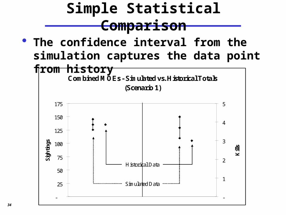
Combined MOEs - Simulated vs. Historical Totals (Scenario 1)

-

25

50

75

100

125

150

175

Sig

hti

ngs

-

1

2

3

4

5

Kill

s

Historical Data

Simulated Data

Combined MOEs - Simulated vs. Historical Totals (Scenario 1)

-

25

50

75

100

125

150

175

Sig

hti

ngs

-

1

2

3

4

5

Kill

s

Historical Data

Simulated Data

The confidence interval from the simulation captures the data point from history

35

Aggregate the Monthly Data

Mean Monthly U-Boat Sightings (Scenario 1)

0.0

5.0

10.0

15.0

20.0

25.0

30.0

35.0

40.0

45.0

Sigh

ting

s

Historical Data

Simulation Data

Mean Monthly U-Boat Sightings (Scenario 1)

0.0

5.0

10.0

15.0

20.0

25.0

30.0

35.0

40.0

45.0

Sigh

ting

s

Historical DataHistorical Data

Simulation DataSimulation Data

The overall confidence level is near 0!

36

New Test for Validation

Efron (1979) first proposed the concept of re-sampling

Well accepted technique Particular use in this test is

somewhat different Note use of bootstrap to

create multiple samples for subsequent comparative uses

Then employ the sign test, a non-parametric test, as a means to compare the real and the simulated data

Run Simulationm time periods

n iterations

Resample fromhistoric data

m per samplen samples

Perform sign test1 resample vs. 1

iterationn comparisons

37

Historical-Based BootstrapTrial Oct 42 Nov 42 Dec 42 Jan 43 Feb 43 Mar 43

1 14 18 10 42 42 42 2 18 14 42 18 19 18 3 18 18 19 18 19 14 4 10 14 14 14 42 14 5 14 19 42 32 42 19 6 42 18 32 32 42 14 7 19 32 14 32 18 19 8 18 14 14 10 14 42 9 18 19 18 42 18 19

10 32 32 32 32 18 18 11 32 10 19 14 10 32 12 10 19 42 32 10 32 13 32 19 19 42 18 18 14 32 32 42 42 42 10 15 10 32 14 18 18 32 16 32 32 10 18 42 14 17 19 19 14 19 19 32 18 32 19 42 18 32 14 19 10 19 19 32 32 32 20 32 42 10 32 42 14

We now compare these values to the simulation values previously provided

38

Bootstrap ResultsTrail T n p–value

1 9 19 0.500 2 9 19 0.500 3 10 20 0.412 4 7 20 0.132 5 9 19 0.500 6 8 19 0.324 7 9 20 0.412 8 14 20 0.021 9 8 19 0.324

10 14 20 0.021 11 11 20 0.252 12 9 20 0.412 13 11 20 0.252 14 10 20 0.412 15 8 20 0.252 16 10 20 0.412 17 12 19 0.084 18 5 20 0.021 19 12 20 0.132 20 12 20 0.132

39

Future Applications

Generalized architecture promotes re-use Coast Guard Deep-water efforts Air Force UAV search in rugged terrain or urban

environments

Human-in-the-loop issues permeate Search and rescue using UAVs Reconnaissance using UAVs Combat missions using UCAVs

Much more that can be done in VV&A

40

Future and Ongoing Efforts

Wish to extend the game theory aspects Would like to do more with the search theory Examining policy adaptation in multi-cultural,

adversarial scenarios Examining employment of agent-based modeling

methods for use in planning and re-planning Examining the use of distillations as a means to

providing real-time decision support to planners

41

Questions?