10-1 nonparametric momentum strategies
TRANSCRIPT

Nonparametric Momentum Strategies
Tsung-Yu ChenNational Central University
Pin-Huang ChouNational Central University
Kuan-Cheng KoNational Chi Nan University
S. Ghon RheeUniversity of Hawai’[email protected]
Current Draft: November 2017

Nonparametric Momentum Strategies
Abstract
Nonparametric measures, such as the rank and sign of daily returns, capture investor underreaction while mitigating overreaction to extreme movements of stock prices. Alternative momentum strategies formed on the basis of such measures, or nonparametric momentum strategies, outperform both Jegadeesh and Titman’s (1993) price momentum and George and Hwang’s (2004) 52-week high momentum, and exhibit no long-term return reversals. The profits, however, are not fully explained by common risk-based asset pricing models, and exhibit patterns consistent with the salience theory proposed by Bordallo, Gennaioli, Shleifer (2012, 2013). In particular, the nonparametric momentum, in conjunction with the 52-week high momentum, subsumes the price momentum, thus suggesting that the price momentum is driven by investor underreaction rather than continued overreaction.
JEL Classification: G12; G14.Keywords: Nonparametric momentum; Rank; Sign; Price momentum; 52-week high momentum.

1
1. Introduction
The search for profitable trading strategies has been a topic of enduring interest to both
practitioners and academics. To date, the price momentum strategy proposed by Jegadeesh and
Titman (JT) (1993) remains one of the most robust trading strategies applied to markets around
the world. However, none of the past studies has questioned the weakness of the parametric nature
of computing past returns in determining winners and losers. This question is critically important
because parametric statistics built on sample mean and variance are highly sensitive to the presence
of extreme observations or outliers (Wright, 2000; Gibbons and Chakraborti, 2010; Hollander,
Wolfe, and Chicken, 2014). As Bordalo, Gennaioli, and Shleifer (BGS) (2012, 2013) point out,
salient features of stock prices could be the cause of mispricing. We believe that the parametric
nature of past and future returns simply magnifies this mispricing problem in asset valuation.
We propose nonparametric momentum (NPM) strategies and investigate their profitability.
NPM strategies are constructed on the basis of daily rank or sign over the formation period.1 Our
choice of these strategies is motivated by the theory of nonparametric statistics, which is known
to be robust to the presence of extreme observations. Nonparametric performance measures,
calculated based on rank and sign, mitigate the impact of extreme returns in the sample, thereby
providing better and more stable predictability of future returns than parametric measures.
Our empirical results fully support the predictions. First, NPM strategies outperform two
well-known momentum strategies, namely the price momentum strategy of JT and the 52-week
high (52wh) momentum strategy of George and Hwang (GH) (2004). Over the five-year holding
1 We use the standardized rank among stocks to obtain its rank measure and the frequency of return on stock that is positive to acquire its sign measure. As the results based on rank and sign measures are quite similar, we mainly focus on rank momentum in this paper but present summary results of the sign momentum in Appendix B. Throughout this paper, we use NPM and rank momentum interchangeably.

2
period following formation, the NPM strategy generates an average monthly profit of 0.352%
outside of January; the profits of JT’s price momentum strategy and the GH’s 52wh momentum
strategy are statistically insignificant. Second, NPM strategies also earn significant profits for one
year following formation, and the profits remain robust after returns are risk-adjusted using either
the Fama and French (FF) (1993) three-factor model or the macroeconomic factor model of Chen,
Roll, and Ross (CRR) (1986).
Why do NPM strategies work better? Over the past few decades, there has been ample
evidence that investors pay attention to only a subset of available information because they do
have limited information processing capacity (Hirshleifer and Teoh, 2003; Peng and Xiong, 2006)
and rely heavily on rules and heuristics to make decisions (Kahneman, 2011). Sometimes they
overreact and sometimes they underreact. Kahneman and Tversky (1979) demonstrate that people
tend to overweight rare events and underweight regular events (Barberis, 2013). Daniel, Hirshleifer,
and Subrahmanyam (1998) show that investors overreact to private information but underreact to
public information because of overconfidence and biased self-attribution. BGS (2012, 2013)
propose the salience theory, in which people’s attention is drawn to the payoffs that are most
different or salient relative to the average. When making choices, they overweight these salient
payoffs relative to their objective probabilities.
A consequence of investor misreaction to information is that stock prices may not properly
reflect stocks’ fundamentals: Observations with extreme returns (positive or negative) are likely to
be driven by investor overreaction to salient news, whereas those with small and insignificant
returns are likely to be driven by investor underreaction to non-salient events. Our nonparametric
measures which curtail the impact of salient extreme returns while assigning a higher weight to

3
the non-salient observations capture the non-salient information in stock prices that is largely
overlooked by investors.
In contrast, JT’s price momentum is constructed on the basis of average past returns; the
predictability of future returns is obscured by extreme returns. Our empirical evidence indicates
that after controlling for nonparametric and 52wh momentum, the price momentum only yields
negative returns, because both price winners and price losers are associated with “salient” return
observations. Similarly, securities with higher positive skewness and extreme positive returns tend
to have lower average returns (Boyer, Mitton, and Vorkink, 2010; Bali, Cakici, and Whitelaw,
2011). Thus, investors in aggregate appear to overreact to extreme past asset returns, and
parametric measures such as mean, variance, and skewness are sensitive to extreme observations
in the sample.
There are at least two interesting findings associated with NPM. First, it is not associated with
any long-term reversals, which thereby eliminates the well-known overreaction phenomenon.
Rather, we observe that NPM profitability is an underreaction-only phenomenon. In addition,
contrary to Lakonishok, Shleifer, and Vishny (1994) and Daniel et al. (1998), there is no over-
extrapolation on past performance for NPM. Second, the persistence of NPM profits comes mainly
from the short leg (or rank losers). This influence is not particularly surprising because it may be
costly to engage in short-selling to exploit the mispricing of rank losers.
What is most amazing is that when we simultaneously compare the competing performance
of the three momentum strategies, the short-term price momentum profitability widely
documented in past literature completely vanishes. What remains is long-term return reversal,
which nevertheless disappears under the CRR risk adjustment. The findings echo GH’s (2004)
claim that short-term profitability and long-term return reversals are two separate phenomena.

4
Moreover, NPM profitability is consistent with investor underreaction predicted by the theories of
Barberis, Shleifer, and Vishny (1998) and Hong and Stein (1999), rather than by continued
overreaction as suggested by Daniel et al. (1998). This issue will be examined in greater detail in
Section 4.
After we confirm that neither the FF (1993) three-factor model nor the CRR (1986)
macroeconomic factor model explains NPM profitability, we propose two sets of behavioral
hypotheses to gain a better understanding of its profits. First, if NPM profitability captures the
non-salient aspect of information embedded in stock returns, we expect it to be less prominent
among stocks with higher salient features, as suggested by BGS (2013). Second, if NPM
profitability is behavioral in nature, we expect it to be stronger and more persistent among stocks
that are subject to higher degrees of arbitrage risk (Ali, Hwang, and Trombley, 2003; Lam and Wei,
2011). We find strong supportive evidence for the above hypotheses.
Overall, our empirical results verify that nonparametric measures capture the non-salient
component of the information neglected by investors, thus contributing to the literature on
momentum investment strategies. Our study has important implications. Although it has been well
documented that stock returns tend to be positively skewed and leptokurtic (Albuquerque, 2012),
our findings indicate that parametric risk measures and moments do not sufficiently summarize all
the information embedded in stock prices.
The remainder of this article proceeds as follows: Section 2 describes the data and
construction of non-parametric momentum measures, and it presents preliminary results regarding
the performance of rank-sorted portfolios. Section 3 compares the performance of three
representative momentum strategies: price momentum, 52wh momentum, and NPM. Section 4

5
outlines two sets of behavioral hypotheses related to NPM profitability, and Section 5 presents our
conclusions.
2. Performance of nonparametric momentum strategies
2.1. Data and nonparametric measures
Our sample consists of the ordinary common equities of all firms (with share codes of 10 and
11) listed on NYSE, AMEX, and NASDAQ for the sample period of January 1963 to December
2015. We obtain market data, including daily returns, monthly returns, share prices, and market
equities, from the Center for Research in Security Prices (CRSP) database and retrieve accounting
data from the COMPUSTAT database. To be included in our sample, a stock must have available
market and accounting data.
We consider a nonparametric measure based on ranks. Let , denote stock i’s daily return
on day d, and denote the number of stocks on day d. We define ( , ) as the rank of ,
among the stocks ( , , … , , ) on day d in ascending order. We assign ties with an
average rank. For example, if two stocks with equal returns are ranked third and fourth, they are
both assigned an average rank of 3.5. Before calculating a firm’s average rank over a formation
period, we first calculate its standardized rank for each trading day, expressed as follows (Wright,
2000):
, = ,
+ 1
2/( 1)( + 1)
12. (1)

6
The daily ranks are then averaged every month and summed over the p-month formation period,
which gives a firm’s average rank, , ( ): 2
, ( ) =1
(1
, ), (2)
where is the number of trading days in month j. The , ( ) measure is calculated on the
basis of the number of available observations. We focus on the formation period of six months, or
p = 6.3
2.2. Portfolio approach to nonparametric momentum strategies
We adopt the portfolio approach used by JT and GH to investigate the performance of NPM
strategies. We sort all stocks into five quintile portfolios based on their average ranks defined in
Equation (2) and construct a NPM strategy by buying the stocks in top quintile portfolio (referred
to as rank winners) and short selling those in the bottom portfolio (referred to as the rank losers);
the long-short portfolio is held for up to five years. Let portfolio 1 (Q1) and portfolio 5 (Q5),
respectively, denote the rank loser and winner portfolios. All portfolios are constructed with equal
weights and held for the subsequent K months with one-month skip. Because JT’s approach
involves an overlapping procedure, we average the portfolio return for each month across K
separate positions, each formed in one of the K consecutive prior months from t K to t 1. In
addition to NPM, we follow JT and GH to construct the two alternative momentum strategies as
comparisons.4
2 As a common practice to alleviate potential microstructure problems associated with the bid-ask bounce, we skip one month between the formation and holding periods when forming the portfolios.3 We also conduct the same analysis based on a formation period of 12 months. The results are generally similar, except that the patterns and their statistical significance are slightly weaker.4 The JT momentum is constructed based on a stock’s past 6-month average return, while the GH momentum is

7
With all months included, Panel A of Table 1 reports the average monthly returns of the three
momentum strategies for one-year to five-year holding period subsequent to portfolio formation.
The performance of both NPM and JT momentum strategies are profitable at 0.442% and 0.309%
per month, respectively, for the first year, but they reverse to become negative and significant for
JT momentum but negative and insignificant for NPM thereafter. This pattern is consistent with
the price momentum compiled by JT, which also exhibits short-term continuation but significant
long-term reversals. As comparisons, the GH strategy generates a positive but insignificant return
of 0.151% per month for the first year and negative, significant returns of -0.480% and -0.397%
per month for second- and third-year holding periods.
[Insert Table 1]
Panel B indicates that three momentum strategies show much larger one-year profits outside
of January than those with January included. The underlying reason is obvious. Investors sell loser
stocks to realize tax loss benefits at year-end, depressing prices of those losers but the prices
rebound in January as the selling pressure weakens. Because momentum strategies take short
positions in loser stocks, price recovery in January increases potential loss. With January excluded,
it is natural that all three momentum profits should be larger than those with January included. The
fact that NPM is subject to the tax-loss-selling effect is not surprising because the phenomenon is
associated with capital losses of individual stocks and our rank measure is constructed on the basis
of individual stocks. Although the three strategies all exhibit reversals in January, the NPM strategy
still remains the most profitable when January observations are excluded. The most interesting
finding is that the long-term reversal pattern disappears for all three momentum strategies,
indicating that long-term reversals are related primarily to January seasonality. Specifically, NPM
constructed based on a stock’s 52wh ratio, which is the closing price at the end of previous month divided by the highest price over past 52 weeks ending in previous month.

8
profits are uniformly positive over longer holding periods following formation; the average
monthly profit is 1.075% (t-statistic = 5.36) for the first year. Even for the entire five-year holding
period, the average monthly profit is still 0.352% (t-statistic = 2.34), suggesting that NPM
profitability is not driven by investor overreaction because there is no occurrence of return
reversals. The return patterns of JT and GH strategies outside of January are generally similar to
NPM except for the slightly smaller profits in the first year and insignificant profits for the entire
5-year holding period.
Overall, this analysis indicates short-term performance persistence for the three momentum
strategies, especially outside of January. So far, each of the three strategies is examined in isolation
from other strategies. Because the three strategies seem to share similar patterns in terms of short-
term profitability and January reversals, it is important to examine the comparative performance
of the three momentum strategies simultaneously by controlling for various confounding factors.
By doing so, we are able to observe whether the NPM strategy plays the determinant role in
generating momentum profits. We formally investigate this issue in next section.
3. Comparison of three representative momentum strategies
3.1. Price momentum, 52-week high momentum, and NPM strategies
Thus far, our empirical results show that the NPM strategy yields short-term profits, and there
are no long-term reversals. The return pattern is different from that of JT’s price momentum profits
but is similar to that of the 52wh momentum profits reported by GH. However, it remains unclear
whether the NPM outperforms the two conventional strategies in generating future return
predictability. Thus, it is important to compare the relative profitability of the three strategies

9
simultaneously. In this section, we explore how the NPM strategy contrasts with price momentum
and 52wh momentum strategies. We estimate the following cross-sectional regressions:
, = , + , , + , , + , , + , ,
+ , 52 , + , 52 , + , , + , , + , . (3)
where , is stock i’s return in month t. The variable , ( , ) is the NPM
winner (loser) dummy, which takes the value of 1 if stock i’s average rank performance is ranked
in the top (bottom) 30% in month t j; , ( , ) is the price winner (loser)
dummy, which takes the value of 1 if stock i’s past six-month average return is ranked in the top
(bottom) 30% in month t j, and 0 otherwise; 52 , (52 , ) is the 52wh winner (loser)
dummy, which takes the value of 1 if ,
,is ranked in the top (bottom) 30% in month t j,
and 0 otherwise. In addition, , and , are the return and market capitalization of
stock i in month t 1, which are included to control for the microstructure effect due to bid-ask
bounce and the size effect.
As in Table 1, the regressions are performed over the holding periods of 12 months (j = 1,...,
12 to 37,..., 48) and 60 months (j = 1,..., 60), respectively. For instance, for the 60-month holding
period, we estimate 60 cross-sectional regressions for j = 1 to j = 60 in month t and then average
the corresponding coefficient estimates. Thus, the return of the “pure” rank winner (loser) portfolio
with the 60-month holding period in month t is calculated as , = , (and , =
, ), and the difference between , and , is the profit of the NPM strategy. The
t-statistics of the coefficient estimates are adjusted using the Newey-West (1987) robust standard
errors.

10
Note that unlike common Fama-MacBeth regression applications where variables of interest
normally take the form of continuous variables, dummy variables are used in this regression. As a
result, the coefficients of dummy variables capture the “net” return of the portfolio related to that
particular dummy variable. For example, , captures the average return of the rest of the
sample stocks (i.e., the “medium” portfolio) that are neither winners nor losers, which are formed
in month t j and held in month t. Thus, , and , capture the incremental returns of rank
winner and loser portfolios, respectively, over the medium portfolio. A major advantage of the
regression approach over the traditional portfolio formation method as used in JT is that it can
filter out the confounding effects such as the size effect and the bid-ask bounce. A second
advantage of this method, as we demonstrate later, is that we can compare the performances of
various holding periods simultaneously. The regression results in Table 2 indicate that: (i) the NPM
strategy has the strongest performance persistence among the three strategies; and (ii) the 52wh
momentum strategy exhibits short-term persistence, but the price momentum totally disappears.
[Insert Table 2]
1. NPM: The most notable finding is that outside of January, NPM profitability is even stronger
and more persistent after controlling for the effects of the other two momentum strategies.
When January observations are excluded, the NPM strategy yields an average return of
0.640% (t-statistic = 5.04) per month for the first year and 0.332% (t-statistic = 2.93) per
month for the entire five-year holding period. More importantly, profits persist across the
entire five-year holding period. NPM profits outside of January for the holding period from
the first to the fourth year are 0.640%, 0.305%, 0.273%, and 0.270%, respectively; all are
statistically significant. In addition, profitability mainly comes from the persistent
underperformance of the rank losers.

11
2. 52wh momentum: The 52wh momentum strategy yields a short-term profit of 0.398% (t-
statistic =2.41) per month in non-January observations, and no long-term reversals occur. The
return patterns are consistent with the findings of GH except that the profitability of the 52wh
momentum strategy is slightly weaker after controlling for the NPM effect.
3. Price momentum: Perhaps the most striking finding is that by controlling for the other two
strategies, price momentum completely disappears, regardless of the inclusion of January
observations. The price momentum profit (excluding January) is 0.094% (-0.023%) for the
first year; both are statistically insignificant. What remains is a long-term reversal pattern:
Outside of January, price momentum yields an average negative return of -0.194% (t-statistic
= -1.66) per month for the entire five-year holding period; the returns of price momentum
from the second to the fourth year are -0.296%, -0.245%, and -0.204%, respectively, and all
are statistically significant. Although we are not yet aware why NPM momentum and 52wh
momentum in combination explain the short-term price momentum, our empirical results
support GH’s (2004) argument that short-term momentum and long-term reversals are two
separate phenomena.
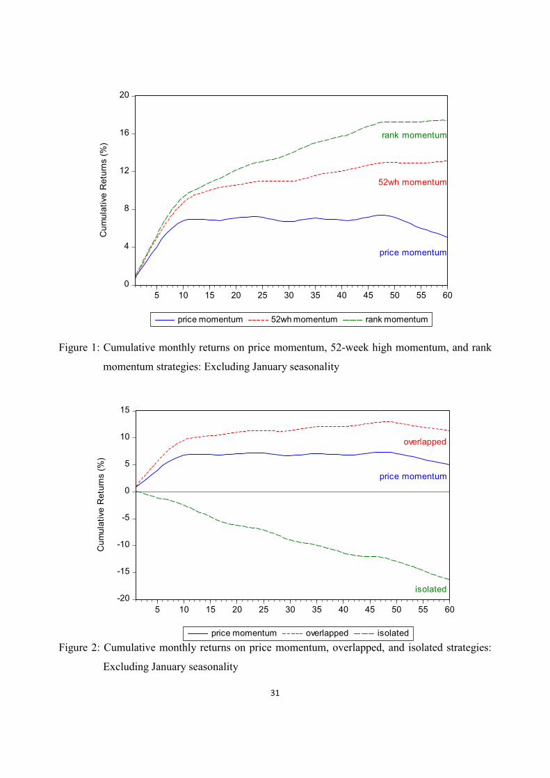
Figure 1 presents the cumulative returns over a 60-month holding period for price momentum,
52wh, and NPM strategies based on the estimates from Equation (3). To avoid January seasonality,
we exclude January observations in calculating the cumulative returns. As seen from Figure 1,
NPM outperforms the other strategies over the entire five-year holding period, followed by the
52wh momentum; price momentum displays the worst performance of the three.
[Insert Figure 1]

12
3.2. Disappearing price momentum?
The most intriguing observation from Table 2 is that the short-term profitability of price
momentum is fully explained jointly by NPM and 52wh momentum. An immediate question to be
resolved is what happens to the short-term profitability of price momentum when we consider only
either 52wh momentum or NPM, but not both?
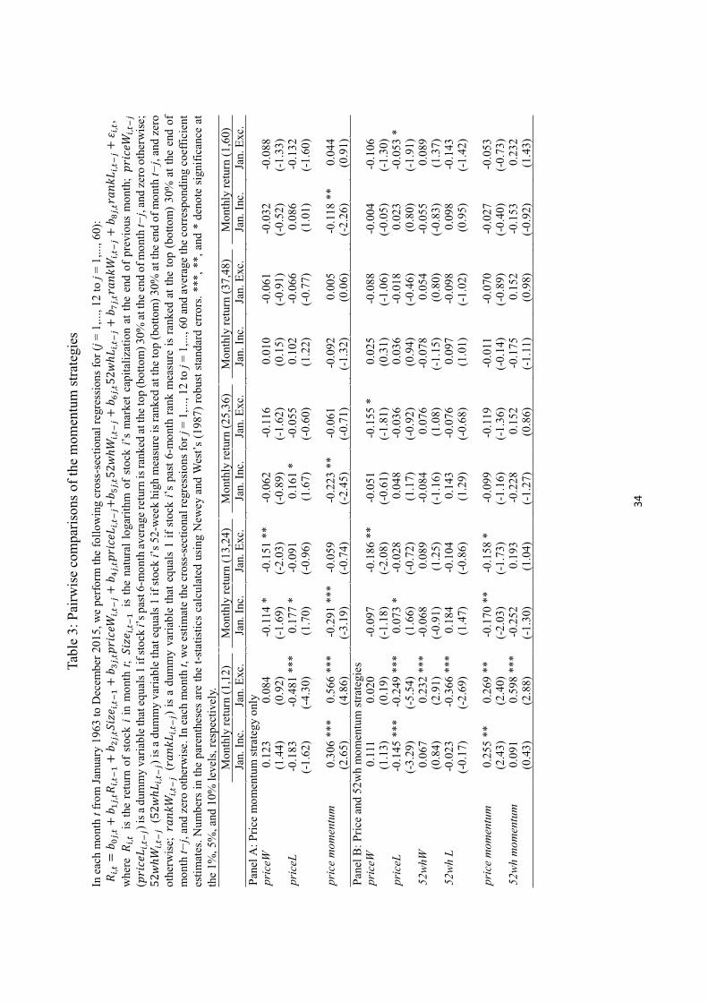
To address this question, we follow the following step-by-step approach. First, we perform
the cross-sectional regression of Equation (3) by including , , , , and dummies of
price momentum only. This model specification is similar to that of JT (1993, 2001), but our model
specifically controls for bid-ask bounce effect and the size effect. As Panel A of Table 3 indicates,
price momentum generates significantly positive profits in the first year following formation
regardless of the inclusion of January months. Its profitability reverses to become significantly
negative with January included in the second, third, and the entire five-year period following
formation. The results are consistent with those of JT, which is expected.
[Insert Table 3]
Second, we introduce both dummies of price momentum and 52wh momentum
simultaneously in Equation (3). This model specification is similar to that introduced by GH, but
differs from theirs in that we do not control for the effect of industry momentum proposed by
Moskowitz and Grinblatt (1999). However, our specification allows us to assess the impact of
52wh momentum on price momentum. Consistent with the results of GH, Panel B of Table 3 shows
that 52wh momentum dominates price momentum in the short term when January seasonality is
removed. The profit of price momentum declines to 0.269% from 0.566% in the absence of 52wh
momentum. Nevertheless, 52wh momentum alone does not fully explain the short-term
profitability of price momentum.

13
In the third step, we assess the impact of NPM alone on price momentum. Panel C of Table 3
shows that the short-term profitability of price momentum disappears: the profit of price
momentum declines to 0.050% (with all months included) and 0.041% (without January excluded),
but both of these figures are insignificant. Moreover, the long-term reversals of price momentum
outside of January are enhanced by the inclusion of NPM. This observation highlights that
importance of the nonparametric measure in isolating short-term momentum from long-term
reversals.5 More importantly, we only need to rely on NPM to explain the return patterns of price
momentum.
The fact that NPM and 52wh momentum in combination explain the short-term momentum
profitability suggests that the three strategies are highly interrelated. Indeed, within our sample,
the overall correlation between past six-month returns and rank is 0.634 and is 0.500 between past
6-month returns and 52wh ratios. 6 Such high correlations motivate us to investigate the
proportions of price winners (losers) that overlap 52wh and/or rank winners (losers). As Panel A
of Table 4 shows, on average 62.29% of price winners are rank winners, and 72.68% of price
winners are either rank winners or 52wh winners. Results for price losers are reported in Panel B;
66.87% of price losers are rank losers, and up to 79.65% of price losers are either rank losers or
52wh losers.
[Insert Table 4]
An interesting question arises: do overlapped or isolated winners and losers of price
momentum behave differently in generating momentum profitability? To answer this question, we
break down price momentum stocks into two categories: (i) one category whose membership
5 Because the 52wh measure is constructed based on the highest price over past 52 weeks, which is the maximum in essence, the information embedded in this measure is more likely to be parametric-based.6 Analogously, the average correlation between 52wh ratios and rank is 0.609. The correlations are first calculated across all stocks in a month, and then averaged over the entire sample.

14
overlaps with rank or 52wh momentum stocks; and (ii) the other category whose membership is
unrelated to rank or 52wh momentum stocks. We refer to the former as the “overlapped” category
of price momentum stocks and the latter as the “isolated” category of price momentum stocks. In
Figure 2, we plot the cumulative returns of the two categories of stocks relative to the entire price
momentum stocks.
[Insert Figure 2]
The most intriguing finding is that the “isolated” category of price momentum stocks
experiences downward performance from the beginning of the five-year horizon of the holding
period. This category of price momentum stocks do not show a long-term reversal pattern that
starts after one or two years following formation as compiled by Jegadeesh and Titman (2001). In
contrast, the “overlapped” category of price momentum stocks shows superior and more persistent
profitability than the isolated category and the standard price momentum. In particular, this
category of price momentum stocks experiences upward performance up to four years, followed
by slight reversal in the 5th year after the portfolio formation.7
Overall, the empirical results indicate that the NPM outperforms the other two forms of
momentum strategies, and that rank measure helps discriminate momentum from reversal patterns
implied by past six-month returns.
3.3. Can nonparametric momentum profits be explained by risk?
In this subsection, we examine whether NPM profits can be explained by risk-based theories.
To this end, we consider two well-known asset-pricing models that have been used in prior
7 Taking a closer look at winner and loser stocks of “overlapped” and “isolated” categories, we find that “overlapped”winners consistently outperform price momentum winners and “isolated” winners while “overlapped” losers consistently underperform price momentum losers and “isolated” losers, generating the return difference between “overlapped” and “isolated” categories of price momentum stocks.

15
literature to evaluate the performance of the price momentum strategy: FF’s (1993) three-factor
model and CRR’s (1986) macroeconomic factor model (the CRR model).8
Our use of the CRR model is justified because Liu and Zhang (2008) demonstrate that the
growth-related macroeconomic factor on industrial production, denoted MP, explains more than
half of price momentum profit. Their empirical results echo the findings of Chordia and
Shivakumar (2002) and Cooper, Gutierrez, and Hameed (2004), who show that price momentum
profits are strong in economic expansions, but not in recessions. Therefore, it is of interest to
examine whether NPM profits can be attributed to fundamental economic forces.9
We estimate the risk-adjusted portfolio returns using the intercepts from time series
regressions of monthly returns of the portfolios (the average coefficient of the corresponding
dummy variable) on the contemporaneous factors. The empirical results are reported in Table 5.
Panel A reports the results based on the FF risk adjustment; Panel B reports the results based on
the CRR risk adjustment.10
[Insert Table 5]
Panel A of Table 5 shows that the NPM profitability remains mostly intact under the FF risk
adjustment. We observe that NPM profits are even stronger for all holding period horizons. Panel
B reveals several interesting features under the CRR adjustment. First, NPM profits remain highly
8 When the FF (2015) five-factor model is used, the results are similar to the results in Table 6.9 Note, however, that the CRR model in its original form is not a pricing model, but a return generating process in the spirit of Ross’s (1976) arbitrage pricing theory. To come up with a pricing formula, we need to estimate the factor risk premium associated with each of the macroeconomic factors. Following Liu and Zhang’s (2008) research design, we first choose 10 size, 10 book-to-market, and 10 momentum one-way sorted portfolios as the testing assets. For each month from January 1963 to November 2015, factor loadings are estimated for each testing asset over the prior 60 months. Fama-MacBeth cross-sectional regression of portfolio returns on the factor loadings is then estimated, which gives the estimates of factor risk premiums. The factor risk premiums are plugged back into the factors, resulting in the “estimates” of the factor portfolios.10 The data for the FF three factors are obtained from Kenneth French’s data library: http://mba.tuck.dartmouth.edu/pages/faculty/ken.french/. The data for CRR factors are downloaded from Xiaolei Liu’s website at http://www.bm.ust.hk/~fnliu/research.html. To conserve space, we report the coefficients of NPM only.

16
significant throughout the five-year holding period, but the CRR model explains approximately
half of NPM profits. For example, the non-January raw NPM profit reported in Table 2 is 0.640%
for the first year but drops to 0.298% for the first year under the CRR risk adjustment. For the
entire 5-year holding period, the risk-adjustment non-January profit is 0.127%, which is only
approximately one-third of the original profit (which is 0.332%, see Table 2).
On the basis of reported findings, we find strong and persistent NPM profitability that is
independent of existing momentum strategies and cannot be fully explained by common risk-based
models. In the following section, we apply behavioral perspectives.
4. Sources of nonparametric momentum profits: Tests of behavioral
hypotheses
So far, we have documented strong and persistent NPM profits that cannot be fully explained
by well-known asset-pricing models; we have also shown that rank losers experience stronger
return persistence than rank winners. In this section, we investigate the sources of NPM
profitability from a behavioral perspective. Nonparametric measures, such as ranks and signs, are
well-known for being less sensitive to the presence of extreme observations in the sample. BGS
(2013), for example, argue that investors’ attention tends to be drawn to assets whose payoffs are
most different or salient relative to an average benchmark. Their trading thus causes stocks with
salient positive (negative) payoffs to be overpriced (underpriced). This is where the unique
property of NPM measures plays a unique role in assessing momentum strategies: rank measures
highlight the relatively non-salient information in the sample while mitigating the effect of salient
features of stock price movements. Moreover, because NPM profitability can not be explained by

17
risk-based theories, it seems plausible that such profitability is the result of investors’ neglect and
is therefore underreaction to non-salient information embedded in stock prices.
If NPM profits are truly behavioral, there are at least two dimensions that can be examined
empirically. First, rank-related performance persistence should be more prominent for stocks with
weaker salience features. Second, if the source of the profitability is behavioral in nature,
performance persistence should also be stronger for stocks that are subject to a higher degree of
arbitrage risk (e.g., Ali et al., 2003; Lam and Wei, 2013).
We test the above two behavioral hypotheses. To elucidate the nature of the NPM effect,
however, we begin with a preliminary analysis of the characteristics of rank-sorted portfolios.
Because rank is a nonparametric measure, it is interesting to understand whether and how it relates
to distribution of returns. Also, we observe whether stocks with similar rank values exhibit similar
firm characteristics that have been documented to be important determinants of momentum and
the cross-section of stock returns.
4.1. The characteristics of rank-sorted portfolios
Table 6 reports descriptive statistics and firm characteristics for stocks in the rank-sorted
quintile portfolios, with the highest rank observations in portfolio Q5 and the lowest rank
observations in portfolio Q1. In Panel A, we report the average descriptive statistics for the rank
quintile portfolios. For each month, we calculate the standardized rank and the first to the fourth
moments for each stock in a quintile portfolio using daily returns over the previous six months.
Each of the descriptive statistics is averaged across stocks in a quintile portfolio and then averaged
over the sample period. In addition to basic descriptive statistics, we also report the average
maximum (Max) and minimum (Min) daily return in the previous month.

18
Panel A reveals a number of interesting patterns across stocks with different ranks. First,
stocks with higher ranks earn higher past returns in terms of mean and median but display a smaller
standard deviation and kurtosis, suggesting that the higher returns of higher-rank stocks are not the
result of their higher risk. Similar to the negative rank-kurtosis relation, lower-rank portfolios also
have higher positive extreme returns Max and lower negative extreme returns Min, indicating that
lower-rank stocks exhibit stronger lottery-like features.11 For example, the lowest- rank portfolio
Q1 has the lowest average monthly return of -0.126% during the formation period, but the largest
Max of 10.252% and the smallest Min of -8.230%.
[Insert Table 6]
Second, there is a U-shaped pattern between skewness and ranks. The average skewness is
smaller for Q3 (0.462) but larger in Q1 (0.697) and Q5 (0.514). This U-shaped relation suggests
that the rank-related return patterns are not simply the result of investors’ preferences for stocks
with positive skewness (Kraus and Litzenberger, 1976; Mitton and Vorkink, 2007).
Panel B reports the average values for market capitalization (Size), book-to-market (BM) ratio,
idiosyncratic risk (Ivolatility), illiquidity measure (Illiq) of Amihud (2002),12 number of analysts
following (Analyst), percentage of institutional ownership (Inst%), and information discreteness
(ID). Detailed variable definitions are given in Appendix A. We use the measures of Ivolatility,
Illiq, Analyst, and Inst% to proxy for arbitrage risk (Ali et al., 2003; Li and Zhang, 2010; Lam and
Wei, 2011). The ID measure is a proxy for limited investor attention and thus captures the degree
of investor underreaction (Da, Gurun and Warachka, 2014).
11 Bali, Cakici, and Whitelaw (2011) show that stocks with higher maximum daily returns Max over the past month earn negative average future returns. There is also a similar inverse, but weaker, relationship between the minimum daily returns Min and future returns, which is subsumed by the negative “maxing out” effect.12 In addition to the Amihud (2002) measure, we also replicate our analyses using the frequency of zero daily return and obtain similar results. Thus, our results are not sensitive to the use of the illiquidity measure.

19
Several interesting patterns emerge in Panel B. First, as rank increases across low-rank to
high-rank portfolios, Size increases but BM ratios decrease, indicating that rank winners (losers)
tend to be large growth (small value) stocks. This pattern implies that the rank-related return
premium is not driven by either the small-firm effect or the value effect. Second, higher-rank
portfolios are characteristics of lower idiosyncratic risk Ivolatility, higher analyst coverage Analyst,
and higher institutional ownership Inst%. In comparison, lower rank portfolios seem to be more
exposed to arbitrage risk than higher rank portfolios.
Third, we observe a concave pattern of Illiq across rank portfolios. This observation suggests
that rank winners and losers are less prone to the illiquidity problem, and that the profitability of
NPM is unlikely to be the result of market fraction. Despite the inverted-U relation between Illiq
and rank measure, rank losers (Q1) have significantly higher values of Illiq than rank winners (Q5),
implying that rank losers are more exposed to arbitrage risk than rank winners. Finally, ID is also
concave across rank portfolios, suggesting rank winners and losers have less discrete information.
More importantly, they seem to exhibit non-salient feature because they demonstrate higher degree
of continuous information that is less salient to investors.
As illustrated by Figure 2 in Section 3.2, the overlapped strategy shows superior and more
persistent profitability while the isolated strategy exhibits downward performance from the
beginning of the 5-year horizon of the holding period. It is possible that the two categories of
stocks exhibit different salient features. In particular, as the overlapped category contains NPM
stocks, this category should demonstrate lower degrees of salient features. The isolated category,
however, is expected to exhibit higher degrees of salient features because this category includes
only pure price momentum stocks. We verify this prediction by reporting descriptive statistics and
firm characteristics for stocks in overlapped and isolated strategies in Table 7.

20
We focus on several salience-related variables. First, isolated winners have higher Skewness
than overlapped winners (1.464 vs. 0.912), indicating that isolated winners are more prone to
positively salient returns. Isolated losers, however, have an average Skewness of -0.380 while
overlapped losers have an average Skewness of 0.184. This evidence suggests that isolated losers
are more prone to negatively salient returns than overlapped losers. Second, the average ID values
are -0.029 and -0.016 for overlapped and isolated winners, respectively. The corresponding ID
values are -0.051 and -0.023 for overlapped and isolated losers, respectively. The observation of
lower values of ID for overlapped components signifies the fact that they are less subject to
investor attention and thus are less salient to investors. The two important findings confirm our
conjecture that salient features are the underlying reason that explains the divergence in return
performance between overlapped and isolated strategies.
[Insert Table 7]
Overall, preliminary results indicate that high rank portfolios exhibit high average returns,
low total volatility, and relatively non-salient features in the past, whereas low-rank portfolios
present high degrees of arbitrage risk. Next, we formally examine the performance of the NPM
strategy by controlling for various confounding factors and explore how various behavioral
hypotheses compete with each other to explain rank-based performance.
4.2. The salience hypothesis
If NPM profitability is driven by investor underreactions to non-salient information
embedded in past stock returns, we expect rank-return predictability to exhibit a salience-related
pattern. In other words, we expect NPM profits to be smaller and weaker for stocks with higher
salience features.

21
Empirically, let _ ( _ ) denote a salience measure for a rank
winner (loser) such that a larger value of _ ( _ ) is associated with
stronger salience; we can perform the following cross-sectional regressions by incorporating
interaction terms into the dummies on rank winners and rank losers:
, = , + , , + , , + , , + , ,
+ , 52 , + , , + , , + , ,
× _ , + , , × _ , + , . (4)
We expect the average estimate of to be negative and the average estimate of to be
positive. Based on BGS’s (2013) idea, we propose three proxies to capture salience:
1. Mean-minus-median. When a winner stock has more observations with positive extreme
payoffs, its mean is greater than its median. Therefore, mean-minus-median serves as a
natural proxy for positive salience _ . Likewise, the negative salience measure
_ , for loser stocks is defined similar to median-minus-mean.
2. Skewness. Positive (negative) skewness reflects assets with positive (negative) salient payoffs
for winners (losers). 13 This measure is conceptually similar to the mean-minus-median
measure, except it is deflated by standard deviation.
3. Information discreteness (ID). This measure, proposed by Da et al. (2014), is defined in
Appendix A. Because a larger ID corresponds to situations where a few extreme positive or
negative observations dominate the overall performance, ID can also serve as a proxy for
salience for both winners and losers.14
13 Empirically, at the beginning of each holding month t, we calculate the mean, median and skewness for each stock using data from the past year ending in month t 1.14 Da et al. (2014) actually use this measure to detect market underreaction. Specifically, they propose a frog-in-the-pan (FIP) hypothesis and claim that ID reflects information that arrives continuously in small amounts, thus capturing investor underreaction.

22
We report the results in Table 8 for holding periods of the first year and the entire five years. Panel
A presents the results based on the positive and negative mean-minus-median measures. Consistent
with the prediction of the salience theory, the coefficient of the interaction term on rank winner
(loser) dummy and salience measure is negative (positive), especially outside of January. For
example, the coefficient of × _ outside of January observations is -0.297 (t-
statistic = -1.30) for the first year and -0.594 (t-statistic = -3.35) for the entire five years; the
coefficient of × _ is 0.503 (t-statistic = 3.14) for the first year and 0.474 (t-
statistic = 4.46) for the entire five years.
[Insert Table 8]
Panel B reports the results based on skewness; the results are similar to those reported in
Panel A. The only difference is that the interaction term on rank loser is statistically significant for
the entire 5 years only and not for the first year holding period. Results based on ID reported in
Panel C of Table 8 also support our salience hypothesis and are consistent with the FIP hypothesis,
thus strengthening our claim that NPM profits are driven by investor underreactions.
4.3. The limits-of-arbitrage hypothesis
Given that our empirical evidence (Table 2) indicates that NPM profitability is primarily
derived from the persistent underperformance of the short leg (i.e., rank losers), a natural emerging
question is why? One good possibility is that the presence of arbitrage limits prevents asset prices
of rank losers from quickly adjusting to their fundamental values.
We can classify such arbitrage limits, or arbitrage risk, into three types: fundamental risk,
noise trader risk, and implementation risk (Barberis and Thaler, 2003). Fundamental risk implies
that investors are uncertain about the true values of the asset (Zhang, 2006). Noise trader risk is

23
present when the market of the asset is populated with irrational traders, whose trading drives an
asset’s price away from its fundamental value (De Long, Shleifer, Summers, and Waldmann, 1990).
Finally, implementation risk pertains to the transaction costs and short-sale restrictions associated
with arbitrage activities.
Empirically, we use analysts’ coverage (Analyst) to proxy the fundamental risk, idiosyncratic
risk (Ivolatility) to proxy noise trader risk, the Amihud measure (Illiq) to proxy potential
transaction costs, and institutional ownership (Inst%) to capture short-sale constraints. Table 9
reports the overall correlations among rank measure and the arbitrage risk proxies. Specifically, in
each month, we first calculate the cross-sectional correlation coefficients for all variables; we next
average the monthly correlation coefficients over the entire sample period. Table 9 shows that rank
is inversely correlated with Ivolatility and Illiq but positively correlated with Analyst and Inst%.
Next, we perform regressions as in Equation (3) by incorporating the interaction terms of rank
winners/losers and each of the four arbitrage risk measures. If arbitrage risk plays a role in driving
NPM, the interaction terms should be significant, especially for rank losers, because arbitrage risks
such as short-sale restrictions are more binding on the short leg.
[Insert Table 9]
To discuss the relation between NPM and arbitrage risk, we invert two variables, Analyst and
Inst%, in the regression model, such that larger variables are associated with a higher arbitrage
limit (Ali, Hwang, and Trombley, 2003). As in Table 8, we focus our analyses on the holding
periods of the first year and the entire five years following formation, as reported in Table 10.
We first focus on the results based on the holding period of the entire five years, as shown in
the right-hand four columns of Table 10. Coefficients on rankL×Ivolatility and rankL×Analyst 1
(Panels A and C) are significantly negative when January observations are excluded. Another

24
striking observation is that coefficients on the interaction terms associated with Illiq (Panel B) are
not significant but with expected signs, confirming our previous argument that NPM momentum
profitability is not induced by the illiquidity problem. In addition, the significance of rank losers
completely disappears or even becomes significantly positive when arbitrage risk is taken into
account, regardless of the inclusion of January observations and price momentum and 52wh
strategies. Again confirming our conjecture, Panel D indicates that coefficients on rankL×Inst% 1
are also all significantly negative. The evidence suggests that the performance persistence of rank
losers is highly related to arbitrage risk and that fundamental risk and noise trader risk are major
sources of risk underpinning the long-term persistence of the NPM.
[Insert Table 10]
Results of the first-year holding period are generally similar to those of the entire five-year
holding period. Coefficients on interaction terms between rank winners and arbitrage risk measures
are insignificant; coefficients on rankL × Inst% 1 are significantly negative. Coefficients on
rankL×Ivolatility and rankL ×Analyst 1 are also significantly negative when January observations
are excluded. These results again confirm that fundamental risk and noise trader risk play
important roles in explaining the return persistence of rank losers.
Overall, the evidence in Table 10 clearly shows that the return persistence of rank losers can
be attributed to arbitrage risk, but this is not the case for rank winners, which is consistent with the
limits-of-arbitrage argument. It also indicates that stock prices continuously deviate from their
fundamental values because of the existence of limits-to-arbitrage, which impedes arbitrageurs in
engaging in arbitrage activities to correct for rank-related mispricing. This further leads to the
long-term persistence of NPM profits.

25
5. Conclusions
We propose nonparametric performance measures (ranks and signs) of past stock returns and
explore whether the measures are associated with future stock returns. Unlike parametric statistics
that have been widely adopted to identify stocks’ past performances, nonparametric statistics are
robust to the presence of outliers in the sample and can account for the non-salient information
embedded in stock prices. Because investors are limited in their attention and information-
processing capacity (Hirshleifer and Teoh, 2003; Peng and Xiong, 2006), we hypothesize that they
tend to underreact to information embedded in nonparametric measures, further inducing
subsequent return continuations.
Our empirical findings generally confirm this prediction. The NPM strategies of buying
stocks with high average ranks (or signs) and shorting those with low average ranks (or signs) are
more profitable, outperforming price momentum and 52wh momentum strategies for the first year
following portfolio formation. When January months are excluded, the profitability of NPM
strategies persists for up to five years and cannot be explained by well-known asset-pricing models.
We further test two sets of behavioral hypotheses to demonstrate that nonparametric measures,
such as rank and sign, capture the non-salient component in stock prices neglected by investors.
First, we show that NPM profitability is weaker among stocks with salient features, suggesting
that NPM is driven by investor underreaction rather than overreaction. Second, the return
persistence of NPM is induced by the higher arbitrage risk of losers, which is consistent with the
limits-of-arbitrage argument.

26
References
Albuquerque, R., 2012. Skewness in stock returns: Reconciling the evidence on firm versus
aggregate returns. Review of Financial Studies 25, 1630-1673.
Ali, A., Hwang, L.-S., Trombley, M.A., 2003. Arbitrage risk and the book-to-market anomaly.
Journal of Financial Economics 69, 355-373.
Amihud, Y., 2002. Illiquidity and stock returns: Cross-section and time-series effects. Journal of
Financial Markets 5, 31-756.
Baker, M., Wurgler, J., 2006, Investor sentitmant and the cross-section of stock returns. Journal of
Finance 61, 1645-1680.
Bali, T.G., Cakici, N., Whitelaw, R.F., 2011. Maxing out: Stocks as lotteries and the cross-section
of expected returns. Journal of Financial Economics 99, 427-446.
Barber, B.M., Odean, T., 2008. All that glitters: The effect of attention and news on the buying
behavior of individual and institutional investors. Review of Financial Studies 21, 785-818.
Barberis, N., 2013. Thirty years of prospect theory in economics: A review and assessment. Journal
of Economic Perspectives 27, 173-195.
Barberis, N., Shleifer, A., Vishny, R.W., 1998. A model of investor sentiment. Journal of Financial
Economics 49, 307-343.
Barberis, N., Thaler, R., 2003. A survey of behavior finance. In: Constantinides, G., Harris, M.,
Stulz, R. (Ed), Handbook of the Economics of Finance. North-Holland, Boston, pp. 1053-
1128.
Bhushun, R., 1994. An informational efficiency perspective on the post-earnings announcement
drift. Journal of Accounting and Economics 18, 45-65.
Bordalo, P., Gennaioli, N., Shleifer, A., 2013. Salience and asset prices. American Economic

27
Review: Papers Proceedings 103, 623-628.
Bordalo, P., Gennaioli, N., Shleifer, A., 2012. Salience theory of choice under risk, Quarterly
Journal of Economics, 127, 1243-1285.
Boyer, B., Mitton, T., Vorkink, K., 2010. Expected idiosyncratic skewness. Review of Financial
Studies 23, 169-202.
Chen, N.-F., Roll, R., Ross, S.A., 1986. Economic forces and the stock market. Journal of Business
59, 383-403.
Chordia, T., Shivakumar, L., 2002. Momentum, business cycle and time-varying expected returns.
Journal of Finance 57, 985-1019.
Cooper, M.J., Gutierrez Jr., R., Hameed, A., 2004. Market states and momentum. Journal of
Finance 59, 1345-1365.
Corwin, S.A., Coughenour, J.F., 2008. Limited attention and the allocation of effort in securities
trading. Journal of Finance 63, 3031-3067.
Da, Z., Gurun, U.G., Warachka, M., 2014. Frog in the pan: Continuous information and momentum.
Review of Financial Studies 27, 2171-2218.
Daniel, K., Hirshleifer, D., Subrahmanyam, A., 1998. Investor psychology and security market
under- and over-reactions. Journal of Finance 53, 1839-1885.
De Long, J.B., Shleifer, A., Summers, L.H., Waldmann, R.J., 1990. Noise trader risk in financial
markets. Journal of Political Economy 98, 703-738.
Fama, E.F., French, K.R., 1992. The cross section of expected stock returns. Journal of Finance
47, 427-466.
Fama, E.F., French, K.R., 1993. Common risk factors in the returns on stocks and bonds. Journal
of Financial Economics 33, 3-56.

28
Fama, E.F., French, K.R., 2015. A five-factor asset pricing model. Journal of Financial Economics,
116, 1-22.
Fama, E.F., MacBeth, J., 1973. Risk, return and equilibrium: Empirical tests. Journal of Political
Economy 81, 607-636.
George, T.J., Hwang, C.-Y., 2004. The 52-week high and momentum investing. Journal of Finance
5, 2145-2176.
Gibbons, J.D., Chakraborti, S., 2010. Nonparametric Statistical Inference, Fifth Edition. Chapman
and Hall/CRC.
Hirshleifer, D., Teoh, S.H., 2003. Limited attention, financial reporting, and disclosure. Journal of
Accounting and Economics 36, 337-386.
Hirst, D.E., Hopkins, P.E., 1998. Comprehensive income reporting and analysts’ valuation
judgements. Journal of Accounting Research 36, 47-75.
Hollander, M., Wolfe, D.A., Chicken, E., 2014. Nonparametric Statistical Methods. John Wiley &
Sons.
Hong, H., Stein, J., 1999. A unified theory of underreaction, momentum trading and overreaction
in asset markets. Journal of Finance 54, 2143-2184.
Jegadeesh, N., Titman, S., 1993. Returns to buying winners and selling losers: Implications for
stock market efficiency. Journal of Finance 43, 65-91.
Jegadeesh, N., Titman, S., 2001. Profitability of momentum strategies: An evaluation of alternative
explanations. Journal of Finance 56, 699-720.
Kahneman, D., 2011. Thinking, Fast and Slow. New York: Farrar, Straus and Giroux.
Kahneman, D., Tversky, A., 1979. Prospect theory: An analysis of decision under risk.
Econometrica 47, 263-291.

29
Kraus, A., Litzenberger, R.H., 1976. Skewness preference and the valuation of risk assets. Journal
of Finance 31, 1085-1100.
Lakonishok, J., Shleifer, A., Vishny, R.W., 1994. Contrarian investment, extrapolation, and risk.
Journal of Finance 49, 1541-1578.
Lam, E.C., Wei, K.C.J., 2011. Limits-to-arbitrage, investment frictions, and the asset growth
anomaly. Journal of Financial Economics 102, 127-149.
Li, D., Zhang, L., 2010. Does q-theory with investment frictions explain anomalies in the cross
section of returns? Journal of Financial Economics 98, 297-314.
Liu, L.X., Zhang, L., 2008. Momentum profits, factor pricing, and macroeconomic risk. Review
of Financial Studies 21, 2417-2448.
Mitton, T., Vorkink, K., 2007. Equilibrium underdiversification and the preference for skewness.
Review of Financial Studies 20, 1255-1288.
Moskowitz, T., Grinblatt, M., 1999. Do industries explain momentum? Journal of Finance 54,
1249-1290.
Newey, W.K., West, K.D., 1987. Hypothesis testing with efficient method of moments estimation.
International Economic Review 28, 777-787.
Peng, L., Xiong, W., 2006. Investor attention, overconfidence and category learning. Journal of
Financial Economics 80, 563-602.
Ross, S.A., 1976. The arbitrage theory of capital asset pricing. Journal of Economic Theory 13,
341-360.
Wright, J.H., 2000. Alternative variance-ratio tests using ranks and signs. Journal of Business and
Economic Statistics 18, 1-9.
Zhang, X.F., 2006. Information uncertainty and stock returns. Journal of Finance 61, 105-136.

30
31
0
4
8
12
16
20
5 10 15 20 25 30 35 40 45 50 55 60
price momentum 52whmomentum rank momentum
CumulativeReturns(%)
rank momentum
52wh momentum
price momentum
Figure 1: Cumulative monthly returns on price momentum, 52-week high momentum, and rank
momentum strategies: Excluding January seasonality
-20
-15
-10
-5
0
5
10
15
5 10 15 20 25 30 35 40 45 50 55 60
price momentum overlapped isolated
CumulativeReturns(%)
overlapped
price momentum
isolated
Figure 2: Cumulative monthly returns on price momentum, overlapped, and isolated strategies:
Excluding January seasonality

32
Table 1: Performance of momentum strategiesFor each month t, we calculate individual stocks’ rank measure (ranki,t(P)) and classify all stocks into quintile portfolios. Stocks with the largest rank measures are placed in portfolio Q5, while those with the smallest rank measures are placed in portfolio Q1. We also follow JT and GH to construct the two alternative strategies. All of the quintile portfolios are rebalanced monthly with the holding period ranging from one year to five years following portfolio formation. Panels A and B report the momentum profits for the full and non-January samples, respectively.Numbers in the parentheses are the t-statistics calculated using Newey and West’s (1987) robust standard errors. ***, **, and * denote significance at the 1%, 5%, and 10% levels, respectively.
Q1 Q2 Q3 Q4 Q5 Q5-Q1Panel A: All monthsNPM1-12 months 0.943 1.244 1.317 1.346 1.385 0.442 ** (2.20)13-24 months 1.404 1.397 1.332 1.260 1.107 -0.297 (-1.54)25-36 months 1.437 1.416 1.341 1.281 1.142 -0.295 (-1.62)37-48 months 1.387 1.374 1.328 1.272 1.206 -0.181 (-1.21)1-60 months 1.322 1.369 1.330 1.281 1.192 -0.130 (-0.83)JT momentum1-12 months 1.089 1.123 1.225 1.319 1.398 0.309 ** (2.16)13-24 months 1.542 1.302 1.266 1.245 1.118 -0.424 *** (-3.65)25-36 months 1.522 1.342 1.266 1.259 1.199 -0.323 *** (-2.92)37-48 months 1.442 1.300 1.259 1.269 1.288 -0.153 * (-1.82)1-60 months 1.420 1.288 1.257 1.261 1.235 -0.185 *** (-2.78)52wh momentum1-12 months 1.193 1.117 1.201 1.293 1.344 0.151 (0.63)13-24 months 1.577 1.347 1.247 1.175 1.098 -0.480 ** (-2.24)25-36 months 1.531 1.436 1.294 1.207 1.134 -0.397 ** (-2.02)37-48 months 1.440 1.406 1.314 1.238 1.178 -0.261 (-1.64)1-60 months 1.444 1.341 1.275 1.232 1.181 -0.263 (-1.49)Panel B: January months excludedNPM1-12 months 0.156 0.737 0.957 1.098 1.231 1.075 *** (5.36)13-24 months 0.659 0.905 0.976 1.001 0.929 0.270 (1.52)25-36 months 0.748 0.941 0.985 1.013 0.939 0.191 (1.09)37-48 months 0.768 0.927 0.981 0.998 0.973 0.205 (1.36)1-60 months 0.640 0.901 0.979 1.017 0.992 0.352 ** (2.34)JT momentum1-12 months 0.333 0.729 0.938 1.048 1.036 0.703 *** (5.04)13-24 months 0.834 0.912 0.977 0.973 0.734 -0.100 (-0.97)25-36 months 0.897 0.957 0.973 0.986 0.787 -0.110 (-1.06)37-48 months 0.880 0.946 0.972 0.985 0.867 -0.012 (-0.14)1-60 months 0.788 0.916 0.970 0.986 0.835 0.048 (0.81)52wh momentum1-12 months 0.332 0.596 0.863 1.079 1.203 0.871 *** (3.68)13-24 months 0.802 0.821 0.898 0.938 0.919 0.118 (0.60)25-36 months 0.852 0.916 0.922 0.949 0.940 0.089 (0.47)37-48 months 0.815 0.922 0.952 0.973 0.949 0.134 (0.82)1-60 months 0.743 0.838 0.921 0.983 0.985 0.242 (1.42)

33
Tabl
e 2:
Com
paris
on o
f thr
ee re
pres
enta
tive
mom
entu
mst
rate
gies
In e
ach
mon
th t
from
Janu
ary
1963
to D
ecem
ber 2
015,
we
perf
orm
the
follo
win
g cr
oss-
sect
iona
l reg
ress
ions
for (
j= 1
,...,
12 to
j=
1,...
, 60)
:,=
,+
,,
+,
,+
,,
+,
,+
,52
,+
,52
,+
,,
+,
,+
,,
whe
re
,is
the
retu
rn o
f st
ock
iin
mon
th t;
,is
the
natu
ral l
ogar
ithm
of
stoc
k i’s
mar
ket c
apita
lizat
ion
at th
e en
d of
pre
viou
s m
onth
;,
(,
) is a
dum
my
varia
ble t
hat e
qual
s 1 if
stoc
k i’s
past
6-m
onth
aver
age r
etur
n is
rank
ed at
the t
op (b
otto
m) 3
0% at
the e
nd o
f mon
th t
j, an
d ze
ro o
ther
wis
e;
52
,(52
,) i
s a d
umm
y va
riabl
e th
at e
qual
s 1 if
stoc
k i’s
52-w
eek
high
mea
sure
is ra
nked
at t
he to
p (b
otto
m) 3
0% a
t the
end
of m
onth
tj,
and
zero
ot
herw
ise;
,(
,)
is a
dum
my
varia
ble
that
equ
als
1 if
stoc
k i’s
pas
t 6-m
onth
ran
k m
easu
re is
ran
ked
at th
e to
p (b
otto
m)
30%
at t
he e
nd o
f m
onth
tj,
and
zero
oth
erw
ise.
In e
ach
mon
th t,
we
estim
ate
the
cros
s-se
ctio
nal r
egre
ssio
ns fo
r j=
1,...
, 12
to j
= 1,
..., 6
0an
d av
erag
e th
e co
rres
pond
ing
coef
ficie
nt
estim
ates
. Num
bers
in th
e pa
rent
hese
s ar
e th
e t-s
tatis
tics
calc
ulat
ed u
sing
New
ey a
nd W
est’s
(198
7) ro
bust
sta
ndar
d er
rors
. ***
, **,
and
* d
enot
e si
gnifi
canc
e at
th
e 1%
, 5%
, and
10%
leve
ls, r
espe
ctiv
ely.
Mon
thly
retu
rn (1
,12)
Mon
thly
retu
rn (1
3,24
)M
onth
ly re
turn
(25,
36)
Mon
thly
retu
rn (3
7,48
)M
onth
ly re
turn
(1,6
0)Ja
n. In
c.Ja
n. E
xc.
Jan.
Inc.
Jan.
Exc
.Ja
n. In
c.Ja
n. E
xc.
Jan.
Inc.
Jan.
Exc
.Ja
n. In
c.Ja
n. E
xc.
Inte
rcep
t1.
319
***
1.02
5**
*1.
329
***
1.01
7**
*1.
338
***
1.01
0**
*1.
307
***
0.98
4**
*1.
338
***
1.02
4**
*(5
.35)
(4.1
9)(5
.32)
(4.1
2)(5
.27)
(4.0
3)(5
.10)
(3.9
0)(5
.49)
(4.2
6),
-0.0
55**
*-0
.045
***
-0.0
56**
*-0
.044
***
-0.0
56**
*-0
.044
***
-0.0
56**
*-0
.044
***
-0.0
56**
*-0
.045
***
(-13
.84)
(-12
.70)
(-13
.60)
(-12
.54)
(-13
.50)
(-12
.40)
(-13
.15)
(-12
.00)
(-13
.98)
(-12
.87)
Size
-3.3
99**
*-1
.401
-2.8
20**
-0.7
10-2
.892
**-0
.739
-2.5
86**
-0.4
59-2
.858
***
-0.7
76(-
2.95
)(-
1.33
)(-
2.48
)(-
0.68
)(-
2.56
)(-
0.72
)(-
2.35
)(-
0.46
)(-
2.63
)(-
0.79
)pr
iceW
0.07
4-0
.064
-0.0
77-0
.217
**-0
.027
-0.1
78*
0.01
9-0
.136
0.00
6-0
.142
(0.6
7)(-
0.56
)(-
0.79
)(-
2.09
)(-
0.28
)(-
1.80
)(0
.19)
(-1.
40)
(0.0
6)(-
1.46
)pr
iceL
-0.0
20-0
.041
0.08
8**
0.07
9**
0.06
2*
0.06
7*
0.04
90.
068
**0.
050
*0.
053
*(-
0.47
)(-
0.91
)(2
.41)
(2.0
7)(1
.75)
(1.8
8)(1
.43)
(2.0
0)(1
.85)
(1.8
9)52
whW
0.02
70.
134
**-0
.050
0.04
7-0
.078
0.02
5-0
.064
0.02
0-0
.047
0.04
4(0
.45)
(2.2
5)(-
0.95
)(0
.95)
(-1.
50)
(0.4
9)(-
1.33
)(0
.42)
(-1.
02)
(0.9
6)52
wh
L0.
028
-0.2
64**
0.19
0*
-0.0
540.
153
-0.0
250.
095
-0.0
660.
103
-0.1
00(0
.24)
(-2.
33)
(1.8
1)(-
0.54
)(1
.63)
(-0.
27)
(1.1
6)(-
0.81
)(1
.19)
(-1.
20)
rank
W0.
037
0.16
7**
*-0
.073
0.06
2-0
.066
0.06
0-0
.030
0.07
7-0
.046
0.07
5(0
.67)
(3.1
4)(-
1.27
)(1
.13)
(-1.
19)
(1.1
0)(-
0.58
)(1
.53)
(-0.
94)
(1.6
0)ra
nkL
-0.3
07**
*-0
.473
***
-0.0
74-0
.244
***
-0.0
52-0
.213
***
-0.0
57-0
.193
***
-0.1
09-0
.257
***
(-3.
79)
(-5.
81)
(-0.
88)
(-2.
94)
(-0.
66)
(-2.
69)
(-0.
78)
(-2.
68)
(-1.
54)
(-3.
64)
pric
em
omen
tum
0.09
4-0
.023
-0.1
65-0
.296
**-0
.089
-0.2
45**
-0.0
31-0
.204
*-0
.044
-0.1
94*
(0.6
7)(-
0.16
)(-
1.36
)(-
2.27
)(-
0.74
)(-
1.98
)(-
0.26
)(-
1.75
)(-
0.39
)(-
1.66
)52
wh
mom
entu
m-0
.001
0.39
8**
-0.2
390.
101
-0.2
310.
050
-0.1
590.
086
-0.1
500.
144
(-0.
01)
(2.4
1)(-
1.58
)(0
.71)
(-1.
64)
(0.3
6)(-
1.29
)(0
.70)
(-1.
16)
(1.1
5)N
PM0.
344
***
0.64
0**
*0.
001
0.30
5**
-0.0
140.
273
**0.
026
0.27
0**
0.06
30.
332
***
(2.6
9)(5
.04)
(0.0
1)(2
.33)
(-0.
11)
(2.1
5)(0
.22)
(2.3
3)(0
.54)
(2.9
3)
34
Tabl
e 3:
Pairw
ise
com
paris
onso
f the
mom
entu
mst
rate
gies
In e
ach
mon
th t
from
Janu
ary
1963
to D
ecem
ber 2
015,
we
perf
orm
the
follo
win
g cr
oss-
sect
iona
l reg
ress
ions
for (
j= 1
,...,
12 to
j=
1,...
, 60)
:,=
,+
,,
+,
,+
,,
+,
,+
,52
,+
,52
,+
,,
+,
,+
,,
whe
re
,is
the
retu
rn o
f st
ock
iin
mon
th t;
,is
the
natu
ral l
ogar
ithm
of
stoc
k i’s
mar
ket c
apita
lizat
ion
at th
e en
d of
pre
viou
s m
onth
;,
(,
) is a
dum
my
varia
ble t
hat e
qual
s 1 if
stoc
k i’s
past
6-m
onth
aver
age r
etur
n is
rank
ed at
the t
op (b
otto
m) 3
0% at
the e
nd o
f mon
th t
j, an
d ze
ro o
ther
wis
e;
52
,(52
,) i
s a d
umm
y va
riabl
e th
at e
qual
s 1 if
stoc
k i’s
52-w
eek
high
mea
sure
is ra
nked
at t
he to
p (b
otto
m) 3
0% a
t the
end
of m
onth
tj,
and
zero
ot
herw
ise;
,(
,)
is a
dum
my
varia
ble
that
equ
als
1 if
stoc
k i’s
pas
t 6-m
onth
ran
k m
easu
re is
ran
ked
at th
e to
p (b
otto
m)
30%
at t
he e
nd o
f m
onth
tj,
and
zero
oth
erw
ise.
In e
ach
mon
th t,
we
estim
ate
the
cros
s-se
ctio
nal r
egre
ssio
ns fo
r j=
1,...
, 12
to j
= 1,
..., 6
0an
d av
erag
e th
e co
rres
pond
ing
coef
ficie
nt
estim
ates
. Num
bers
in th
e pa
rent
hese
s ar
e th
e t-s
tatis
tics
calc
ulat
ed u
sing
New
ey a
nd W
est’s
(198
7) ro
bust
sta
ndar
d er
rors
. ***
, **,
and
* d
enot
e si
gnifi
canc
e at
th
e 1%
, 5%
, and
10%
leve
ls, r
espe
ctiv
ely.
Mon
thly
retu
rn (1
,12)
Mon
thly
retu
rn (1
3,24
)M
onth
ly re
turn
(25,
36)
Mon
thly
retu
rn (3
7,48
)M
onth
ly re
turn
(1,6
0)Ja
n. In
c.Ja
n. E
xc.
Jan.
Inc.
Jan.
Exc
.Ja
n. In
c.Ja
n. E
xc.
Jan.
Inc.
Jan.
Exc
.Ja
n. In
c.Ja
n. E
xc.
Pane
l A:P
rice
mom
entu
m st
rate
gy o
nly
pric
eW0.
123
0.08
4-0
.114
*-0
.151
**-0
.062
-0.1
160.
010
-0.0
61-0
.032
-0.0
88(1
.44)
(0.9
2)(-
1.69
)(-
2.03
)(-
0.89
)(-
1.62
)(0
.15)
(-0.
91)
(-0.
52)
(-1.
33)
pric
eL-0
.183
-0.4
81**
*0.
177
*-0
.091
0.16
1*
-0.0
550.
102
-0.0
660.
086
-0.1
32(-
1.62
)(-
4.30
)(1
.70)
(-0.
96)
(1.6
7)(-
0.60
)(1
.22)
(-0.
77)
(1.0
1)(-
1.60
)
pric
em
omen
tum
0.30
6**
*0.
566
***
-0.2
91**
*-0
.059
-0.2
23**
-0.0
61-0
.092
0.00
5-0
.118
**0.
044
(2.6
5)(4
.86)
(-3.
19)
(-0.
74)
(-2.
45)
(-0.
71)
(-1.
32)
(0.0
6)(-
2.26
)(0
.91)
Pane
l B:P
rice
and
52w
h m
omen
tum
stra
tegi
espr
iceW
0.11
10.
020
-0.0
97-0
.186
**-0
.051
-0.1
55*
0.02
5-0
.088
-0.0
04-0
.106
(1.1
3)(0
.19)
(-1.
18)
(-2.
08)
(-0.
61)
(-1.
81)
(0.3
1)(-
1.06
)(-
0.05
)(-
1.30
)pr
iceL
-0.1
45**
*-0
.249
***
0.07
3*
-0.0
280.
048
-0.0
360.
036
-0.0
180.
023
-0.0
53*
(-3.
29)
(-5.
54)
(1.6
6)(-
0.72
)(1
.17)
(-0.
92)
(0.9
4)(-
0.46
)(0
.80)
(-1.
91)
52w
hW0.
067
0.23
2**
*-0
.068
0.08
9-0
.084
0.07
6-0
.078
0.05
4-0
.055
0.08
9(0
.84)
(2.9
1)(-
0.91
)(1
.25)
(-1.
16)
(1.0
8)(-
1.15
)(0
.80)
(-0.
83)
(1.3
7)52
wh
L-0
.023
-0.3
66**
*0.
184
-0.1
040.
143
-0.0
760.
097
-0.0
980.
098
-0.1
43(-
0.17
)(-
2.69
)(1
.47)
(-0.
86)
(1.2
9)(-
0.68
)(1
.01)
(-1.
02)
(0.9
5)(-
1.42
)
pric
em
omen
tum
0.25
5**
0.26
9**
-0.1
70**
-0.1
58*
-0.0
99-0
.119
-0.0
11-0
.070
-0.0
27-0
.053
(2.4
3)(2
.40)
(-2.
03)
(-1.
73)
(-1.
16)
(-1.
36)
(-0.
14)
(-0.
89)
(-0.
40)
(-0.
73)
52w
hm
omen
tum
0.09
10.
598
***
-0.2
520.
193
-0.2
280.
152
-0.1
750.
152
-0.1
530.
232
(0.4
3)(2
.88)
(-1.
30)
(1.0
4)(-
1.27
)(0
.86)
(-1.
11)
(0.9
8)(-
0.92
)(1
.43)

35
Tabl
e 3
cont
inue
dM
onth
ly re
turn
(1,1
2)M
onth
ly re
turn
(13,
24)
Mon
thly
retu
rn (2
5,36
)M
onth
ly re
turn
(37,
48)
Mon
thly
retu
rn (1
,60)
Jan.
Inc.
Jan.
Exc
.Ja
n. In
c.Ja
n. E
xc.
Jan.
Inc.
Jan.
Exc
.Ja
n. In
c.Ja
n. E
xc.
Jan.
Inc.
Jan.
Exc
.Pa
nel C
:Pric
e an
d N
PM st
rate
gies
pric
eW0.
057
-0.0
76-0
.092
-0.2
26**
-0.0
45-0
.193
*0.
027
-0.1
26-0
.009
-0.1
53(0
.51)
(-0.
65)
(-0.
93)
(-2.
16)
(-0.
46)
(-1.
94)
(0.2
7)(-
1.28
)(-
0.10
)(-
1.57
)pr
iceL
0.00
7-0
.117
*0.
158
***
0.05
60.
127
***
0.06
20.
092
**0.
053
0.10
5**
*0.
034
(0.1
2)(-
1.94
)(3
.19)
(1.2
9)(2
.88)
(1.5
4)(2
.20)
(1.2
6)(3
.26)
(1.1
2)ra
nkW
0.04
40.
231
***
-0.1
000.
082
-0.0
840.
089
-0.0
590.
087
-0.0
680.
097
(0.5
7)(3
.08)
(-1.
30)
(1.1
2)(-
1.15
)(1
.24)
(-0.
86)
(1.3
1)(-
1.01
)(1
.50)
rank
L-0
.316
***
-0.5
75**
*-0
.023
-0.2
68**
-0.0
22-0
.246
**-0
.022
-0.2
14**
-0.0
76-0
.290
***
(-2.
69)
(-4.
81)
(-0.
20)
(-2.
31)
(-0.
20)
(-2.
26)
(-0.
22)
(-2.
23)
(-0.
76)
(-2.
92)
pric
em
omen
tum
0.05
00.
041
-0.2
49**
-0.2
82**
-0.1
71*
-0.2
55**
-0.0
65-0
.179
*-0
.114
-0.1
87**
(0.4
0)(0
.31)
(-2.
43)
(-2.
56)
(-1.
69)
(-2.
48)
(-0.
65)
(-1.
81)
(-1.
29)
(-2.
01)
NPM
0.36
0*
0.80
6**
*-0
.077
0.35
0*
-0.0
630.
335
*-0
.037
0.30
1*
0.00
80.
387
**(1
.92)
(4.3
0)(-
0.41
)(1
.91)
(-0.
35)
(1.9
2)(-
0.23
)(1
.93)
(0.0
5)(2
.42)

36
Table 4: Proportions of stocks in price momentum overlapping rank and 52-week high
momentumThis table reports the average numbers and proportions of price winners (losers) that overlap rank and 52-week high winners (losers). Panels A and B reveal the parts of winner and loser stocks, respectively. We calculate the numbers and proportions of firms for each category at the end of every formation period and average then over our sample period. {price winners} is the number of price winner stocks and {price losers} is the number of price loser stocks. {price winners} rank winners} is the number of price winner stocks that overlap rank winner stocks; {price losers} rank losers} is the number of price loser stocks that overlap rank loser stocks. {price winners} rank winners or 52wh winners} is the number of price winner stocks that overlap rank or 52 week-high winner stocks; {price losers} rank losers or 52wh losers} is the number of price loser stocks that overlap rank or 52 week-high loser stocks.
# of stocks PercentagePanel A: Winners{price winners} 1,388 100%
{price winners} rank winners} 865 62.29%{price winners} rank winners or 52wh winners} 1,009 72.68%Panel B: Losers{price losers} 1,388 100%
{price losers} rank losers} 928 66.87%{price losers} rank losers or 52wh losers} 1,106 79.65%

37
Table 5: Performance of profits from price, 52-week high, and NPM strategies under risk
adjustmentsIn each month t from January 1963 to December 2015, we perform the following cross-sectional regressions for (j =1,..., 12 to j = 1,..., 60):
, = , + , , + , , + , , + , , + , 52 , +
, 52 , + , , + , , + , ,where , is the return of stock i in month t; , is the natural logarithm of stock i’s market capitalization at the end of previous month; , ( , ) is a dummy variable that equals 1 if stock i’s past 6-month average return is ranked at the top (bottom) 30% at the end of month t j, and zero otherwise; 52 ,
(52 , ) is a dummy variable that equals 1 if stock i’s 52-week high measure is ranked at the top (bottom) 30% at the end of month t j, and zero otherwise; , ( , ) is a dummy variable that equals 1 if stock i’s past 6-month rank measure is ranked at the top (bottom) 30% at the end of month t j, and zero otherwise. In each month t, we estimate the cross-sectional regressions for j = 1,..., 12 to j = 1,..., 60 and average the corresponding coefficient estimates. To obtain risk-adjusted returns, we perform time-series regressions of these averages (one for each average) on the contemporaneous FF’s three factors (Panel A) and CRR’s five factors (Panel B) to hedge out the risk exposure. Numbers in the parentheses are the t-statistics calculated using Newey and West’s (1987) robust standard errors. ***, **, and * denote significance at the 1%, 5%, and 10% levels, respectively.
Monthly return (1,12)
Monthly return (13,24)
Monthly return (25,36)
Monthly return (37,48)
Monthly return (1,60)
Jan. Inc. Jan. Exc. Jan. Inc. Jan. Exc. Jan. Inc. Jan. Exc. Jan. Inc. Jan. Exc. Jan. Inc. Jan. Exc.Panel A: Risk-adjusted returns using the FF three-factor modelrankW
0.110 ***
0.195 ***
-0.023
0.074 ** -0.011
0.076 ** 0.018 0.085 ***
0.007 0.088 ***
(2.95)
(5.47) (-0.59)
(2.06)
(-0.30)
(2.25) (0.52) (2.60) (0.22)
(3.12)
rankL
-0.400
***
-0.535 ***
-0.157
***
-0.287
***
-0.127
** -0.248
***
-0.118
** -0.219
***
-0.186
***
-0.298
***
(-7.33)
(-10.94)
(-2.88)
(-5.72)
(-2.53)
(-5.48)
(-2.51)
(-5.21)
(-4.3) (-7.68)
NPM0.511 **
*0.730 **
*0.134 0.361 **
*0.116 0.324 **
*0.136 * 0.304 **
*0.193 **
*0.386 **
*(6.12
)(9.57) (1.54
)(4.59
)(1.46) (4.55) (1.84) (4.55) (2.77
)(6.18
)Panel B: Risk-adjusted returns using the CRR five-factor modelrankW 0.069 ** 0.043 0.001 0.014 0.021 0.032 0.052 * 0.024 0.027 0.017
(2.21) (1.36) (0.04
)(0.44
) (0.70) (1.06) (1.67) (0.80) (1.24)
(0.81)
rankL
-0.256
*** -0.255 **
*-
0.058-
0.060-
0.089 **-
0.093 **-
0.094 **-
0.084 ** -0.12 ***
-0.110
***
(-6.01) (-6.05) (-
1.29)(-
1.39)(-
2.13)(-
2.32)(-
2.29)(-
2.24)(-
3.71)(-
3.64)
NPM 0.326 *** 0.298 **
* 0.059 0.073 0.110 * 0.125 ** 0.146 ** 0.108 * 0.147 *** 0.127 **
*(5.07
) (4.66) (0.91)
(1.15) (1.78) (2.12) (2.34) (1.92) (3.02
)(2.79
)

38
Table 6: Descriptive statistics and firm characteristics of rank quintile portfoliosFor each month t, we calculate individual stocks’ rank measure (ranki,t(P)) and classify all stocks into quintile portfolios. Stocks with the largest rank measures are placed in portfolio Q5, while those with the smallest rank measures are placed in portfolio Q1. Panels A and B report the time-series average values of summary statistics and characteristics calculated on a monthly basis for stocks in rank-sorted quintile portfolios. rank is defined as the average of the past 6-month rank measure; Mean is the average daily return of stocks over the past 6 months; Median is the medium daily return of stocks over the past 6 months; Std. dev. is the standard deviation of each stock computed using daily returns over the past 6 months; Skewness is the skewness of each stock computed using daily returns over the past 6 months; Kurtosis is the kurtosis of each stock computed using daily returns over the past 6 months; Max and Min are the maximum and minimum daily return for each stock in the previous month. From July of each year to June of next year, Size is the market value of equity (in millions of dollars) at the end of June in the current year; BM is the ratio of book value of equity at the end of the previous year divided by market capitalization at the end of the previous year; Ivolatility is the variance of residuals obtained from regressing individual stocks’ daily returns on the value-weighted market index over the past year ending in the previous month with a minimum of 250 trading days; Illiq is the Amihud measure calculated over the past year ending in the previous month; Analyst is defined as the number of analysts following the firm at end of June in the current year, and is set to be zero if a firm is not included in the database; Inst% is defined as the percentage of common stocks owned by institutions at end of June in the current year; ID is the information discreteness measure calculated using data over past year ending in the previous month.The last column reports the difference between Q5 and Q1 with t-statistics reported in parentheses calculated using Newey and West’s (1987) robust standard errors. ***, **, and * denote significance at the 1%, 5%, and 10% levels, respectively.
Q1 Q2 Q3 Q4 Q5 Q5-Q1Panel A: Summary statistic of daily returns over the formation periodrank -0.126 -0.041 0.004 0.047 0.116 0.243 ***
(36.36)Mean -0.150 0.008 0.087 0.159 0.297 0.446 ***
(19.42)Median -0.201 -0.049 -0.011 0.017 0.092 0.293 ***
(4.22)Std. dev. 4.497 3.581 3.109 2.757 2.597 -1.901 ***
(-8.69)Skewness 0.697 0.494 0.462 0.482 0.514 -0.183 ***
(-2.74)Kurtosis 6.324 5.782 5.804 5.673 5.254 -1.069 ***
(-2.93)Max 10.252 7.812 6.692 5.943 5.732 -4.520 ***
(-7.24)Min -8.230 -6.470 -5.497 -4.765 -4.375 3.854 ***
(9.40)Panel B: Firm characteristicsSize (in millions) 555.735 1,138.754 1,455.674 1,736.385 1,838.918 1,283.183 ***
(2.98)BM 0.997 0.972 0.919 0.838 0.685 -0.313 ***
(-6.17)Ivolatility 4.220 3.437 3.012 2.683 2.517 -1.703 ***
(-9.58)ILLIQ 7.176 9.110 8.993 7.309 4.740 -2.436 ***
(-3.68)Analyst 4.689 5.525 6.010 6.661 7.290 2.601 ***
(5.51)Inst% 0.260 0.311 0.332 0.353 0.380 0.120 ***
(7.74)ID -0.056 -0.027 -0.019 -0.021 -0.040 0.016 **
(2.46)

39
Tabl
e 7:
Des
crip
tive
stat
istic
s and
firm
cha
ract
eris
tics o
f ove
rlapp
ed a
nd is
olat
ed st
rate
gies
For e
ach
mon
th t,
we
calc
ulat
e in
divi
dual
stoc
ks’p
ast 6
-mon
th a
vera
ge re
turn
, ran
k m
easu
re, a
nd 5
2-w
eek
high
. W
e cl
assi
fy a
ll st
ocks
into
qui
ntile
por
tfolio
s for
th
e th
ree
mea
sure
s. St
ocks
with
the
larg
est v
alue
s on
each
mea
sure
are
pla
ced
in p
ortfo
lio Q
5, w
hile
thos
e w
ith th
e sm
alle
st v
alue
s on
each
mea
sure
are
pla
ced
in
portf
olio
Q1.
We
defin
e st
ocks
bel
ongi
ng to
pric
e m
omen
tum
Q5
(Q1)
por
tfolio
that
ove
rlap
with
ran
k or
52w
h m
omen
tum
Q5
(Q1)
por
tfolio
s as
ove
rlapp
ed
win
ners
(los
ers)
. Sto
cks b
elon
ging
to p
rice
mom
entu
m Q
5 (Q
1) p
ortfo
lio th
at a
re u
nrel
ated
to ra
nk o
r 52w
h m
omen
tum
Q5
(Q1)
por
tfolio
s are
def
ined
as i
sola
ted
win
ners
(los
ers)
. Pan
els A
and
B re
port
the
time-
serie
s av
erag
e va
lues
of s
umm
ary
stat
istic
s an
d ch
arac
teris
tics
calc
ulat
ed o
n a
mon
thly
bas
is fo
r sto
cks
in ra
nk-
sorte
d qu
intil
e po
rtfol
ios.
rank
is d
efin
ed a
s th
e av
erag
e of
the
past
6-m
onth
ran
k m
easu
re; M
ean
is th
e av
erag
e da
ily r
etur
n of
sto
cks
over
the
past
6 m
onth
s;
Med
ian
is th
e m
ediu
m d
aily
retu
rn o
f sto
cks o
ver t
he p
ast 6
mon
ths;
Std
. dev
.is t
he st
anda
rd d
evia
tion
of e
ach
stoc
k co
mpu
ted
usin
g da
ily re
turn
s ove
r the
pas
t 6
mon
ths;
Ske
wne
ssis
the
skew
ness
of e
ach
stoc
k co
mpu
ted
usin
g da
ily re
turn
s ove
r the
pas
t 6 m
onth
s; K
urto
sisis
the
kurto
sis o
f eac
h st
ock
com
pute
d us
ing
daily
re
turn
s ove
r the
pas
t 6 m
onth
s; M
axan
d M
inar
e th
e m
axim
um a
nd m
inim
um d
aily
retu
rn fo
r eac
h st
ock
in th
e pr
evio
us m
onth
. Fro
m Ju
ly o
f eac
h ye
ar to
June
of
next
yea
r, Si
zeis
the
mar
ket v
alue
of e
quity
(in
mill
ions
of d
olla
rs) a
t the
end
of J
une
in th
e cu
rren
t yea
r; BM
is th
e ra
tio o
f boo
k va
lue
of e
quity
at t
he e
nd o
f the
pr
evio
us y
ear d
ivid
ed b
y m
arke
t cap
italiz
atio
n at
the
end
of th
e pr
evio
us y
ear;
Ivol
atili
tyis
the
varia
nce
of re
sidu
als
obta
ined
from
regr
essi
ng in
divi
dual
sto
cks’
daily
retu
rns o
n th
e va
lue-
wei
ghte
d m
arke
t ind
ex o
ver t
he p
ast y
ear e
ndin
g in
the
prev
ious
mon
th w
ith a
min
imum
of 2
50 tr
adin
g da
ys; I
lliq
is th
e Am
ihud
mea
sure
ca
lcul
ated
ove
r the
pas
t yea
r end
ing
in th
e pr
evio
us m
onth
; Ana
lyst
is d
efin
ed a
s th
e nu
mbe
r of a
naly
sts
follo
win
g th
e fir
m a
t end
of J
une
in th
e cu
rren
t yea
r, an
d is
set
to b
e ze
ro if
a fi
rm is
not
incl
uded
in th
e da
taba
se; I
nst%
is d
efin
ed a
s th
e pe
rcen
tage
of c
omm
on s
tock
s ow
ned
by in
stitu
tions
at e
nd o
f Jun
e in
the
curr
ent
year
; ID
is th
e in
form
atio
n di
scre
tene
ss m
easu
re c
alcu
late
d us
ing
data
ove
r pas
t yea
r end
ing
in th
e pr
evio
us m
onth
. The
last
col
umn
repo
rts th
e di
ffere
nce
betw
een
Q5
and
Q1
with
t-st
atis
tics r
epor
ted
in p
aren
thes
es c
alcu
late
d us
ing
New
ey a
nd W
est’s
(198
7) ro
bust
stan
dard
err
ors.
***,
**,
and
* d
enot
e si
gnifi
canc
e at
the
1%,
5%, a
nd 1
0% le
vels
, res
pect
ivel
y.W
inne
r po
rtfol
ioLo
ser p
ortfo
lioO
verla
pped
Isol
ated
Ove
rlapp
edIs
olat
edPa
nel A
: Sum
mar
y st
atis
tic o
f dai
ly re
turn
s ove
r the
form
atio
n pe
riod
Mea
n0.
348
0.37
1-0
.193
-0.0
78M
edia
n0.
068
-0.0
55-0
.141
-0.0
12St
d. d
ev.
3.07
55.
348
4.05
32.
442
Skew
ness
0.91
21.
464
0.18
4-0
.380
Kur
tosi
s6.
236
8.45
85.
879
6.13
4M
ax7.
261
12.0
048.
856
4.80
9M
in-4
.789
-7.8
51-8
.214
-5.1
10Pa
nel B
: Firm
cha
ract
eris
tics
Size
(in
mill
ions
)1,
901.
225
501.
853
1,06
4.25
91,
869.
815
BM0.
594
0.73
80.
971
0.87
3Iv
olat
ility
3.19
15.
590
4.29
42.
666
ILLI
Q6.
216
17.3
4810
.037
5.85
9An
alys
t6.
456
3.63
35.
006
5.50
6In
st%
0.35
50.
215
0.28
20.
305
ID-0
.029
-0.0
16-0
.051
-0.0
23

40
Tabl
e 8:
Per
form
ance
of N
PMpr
ofits
cond
ition
al o
n sa
lienc
eIn
eac
h m
onth
tfr
om Ja
nuar
y 19
63 to
Dec
embe
r 201
5, w
e pe
rfor
m th
e fo
llow
ing
cros
s-se
ctio
nal r
egre
ssio
ns fo
r (j=
1,..
., 12
to j
= 1,
..., 6
0):
,=
,+
,,
+,
,+
,,
+,
,+
,52
,+
,52
,+
,,
+,
,
+,
,_
,+
,,
_,
+,
,w
here
,
is th
e re
turn
of
stoc
k ii
n m
onth
t;,
is th
e na
tura
l log
arith
m o
f st
ock
i’s m
arke
t cap
italiz
atio
n at
the
end
of p
revi
ous
mon
th;
,
(,
) is a
dum
my
varia
ble t
hat e
qual
s 1 if
stoc
k i’s
past
6-m
onth
aver
age r
etur
n is
rank
ed at
the t
op (b
otto
m) 3
0% at
the e
nd o
f mon
th t
j, an
d ze
ro o
ther
wis
e;
52
,(52
,) i
s a d
umm
y va
riabl
e th
at e
qual
s 1 if
stoc
k i’s
52-w
eek
high
mea
sure
is ra
nked
at t
he to
p (b
otto
m) 3
0% a
t the
end
of m
onth
tj,
and
zero
ot
herw
ise;
,(
,)
is a
dum
my
varia
ble
that
equ
als
1 if
stoc
k i’s
pas
t 6-m
onth
ran
k m
easu
re is
ran
ked
at th
e to
p (b
otto
m)
30%
at t
he e
nd o
f m
onth
tj,
and
zero
oth
erw
ise.
In e
ach
mon
th t,
we
estim
ate
the
cros
s-se
ctio
nal r
egre
ssio
ns fo
r j=
1,...
, 12
to j
= 1,
..., 6
0an
d av
erag
e th
e co
rres
pond
ing
coef
ficie
nt
estim
ates
. _
,an
d _
,ar
est
ock
i’ssa
lienc
e m
easu
re t
akin
g po
sitiv
e an
d ne
gativ
e si
gns,
resp
ectiv
ely.
In
Pane
ls A
, B, a
nd C
, _
,an
d (
_,
) ar
e m
easu
red
by m
ean-
min
us-m
edia
n (m
edia
n-m
inus
-mea
n),s
kew
ness
(ne
gativ
e sk
ewne
ss),
and
ID, r
espe
ctiv
ely.
Num
bers
in th
e pa
rent
hese
s are
the
t-sta
tistic
s cal
cula
ted
usin
g N
ewey
and
Wes
t’s (1
987)
robu
st st
anda
rd e
rror
s. **
*, *
*, a
nd *
den
ote
sign
ifica
nce
at th
e 1%
, 5%
, an
d 10
% le
vels
, res
pect
ivel
y.M
onth
ly re
turn
(1,1
2)M
onth
ly re
turn
(1,6
0)Ja
n. In
c.Ja
n. E
xc.
Jan.
Inc.
Jan.
Exc
.Ja
n. In
c.Ja
n. E
xc.
Jan.
Inc.
Jan.
Exc
.Pa
nel A
: Sal
ienc
e de
fined
by th
e di
ffere
nce
betw
een
mea
n an
d m
ediu
mpr
iceW
0.06
8-0
.065
0.02
2-0
.112
(0.6
9)(-
0.64
)(0
.26)
(-1.
29)
pric
eL-0
.053
-0.0
75*
0.03
80.
038
(-1.
30)
(-1.
79)
(1.5
5)(1
.53)
52w
hW0.
006
0.11
2*
-0.0
610.
028
(0.1
1)(1
.91)
(-1.
34)
(0.6
3)52
wh
L0.
080
-0.2
04*
0.11
5-0
.082
(0.6
8)(-
1.80
)(1
.34)
(-0.
99)
rank
W0.
102
0.30
0**
*0.
069
0.22
0**
*-0
.039
0.13
7**
-0.0
050.
148
**(1
.24)
(3.7
5)(0
.92)
(2.9
6)(-
0.55
)(1
.99)
(-0.
07)
(2.1
8)ra
nkL
-0.1
98*
-0.4
71**
*-0
.191
***
-0.3
36**
*0.
042
-0.1
64*
-0.0
32-0
.159
***
(-1.
80)
(-4.
43)
(-2.
65)
(-4.
96)
(0.4
8)(-
1.95
)(-
0.52
)(-
2.62
)ra
nkW
Pos_
Salie
nce
-0.3
05-0
.442
-0.2
60-0
.297
-0.3
90-0
.719
***
-0.3
90**
-0.5
94**
*(-
0.98
)(-
1.40
)(-
1.15
)(-
1.30
)(-
1.53
)(-
2.77
)(-
2.23
)(-
3.35
)ra
nkL
Neg
_Sal
ienc
e0.
477
***
0.40
6**
0.53
7**
*0.
503
***
0.45
2**
*0.
513
***
0.39
7**
*0.
474
***
(2.6
0)(2
.14)
(3.4
4)(3
.14)
(3.7
9)(4
.12)
(3.9
2)(4
.46)
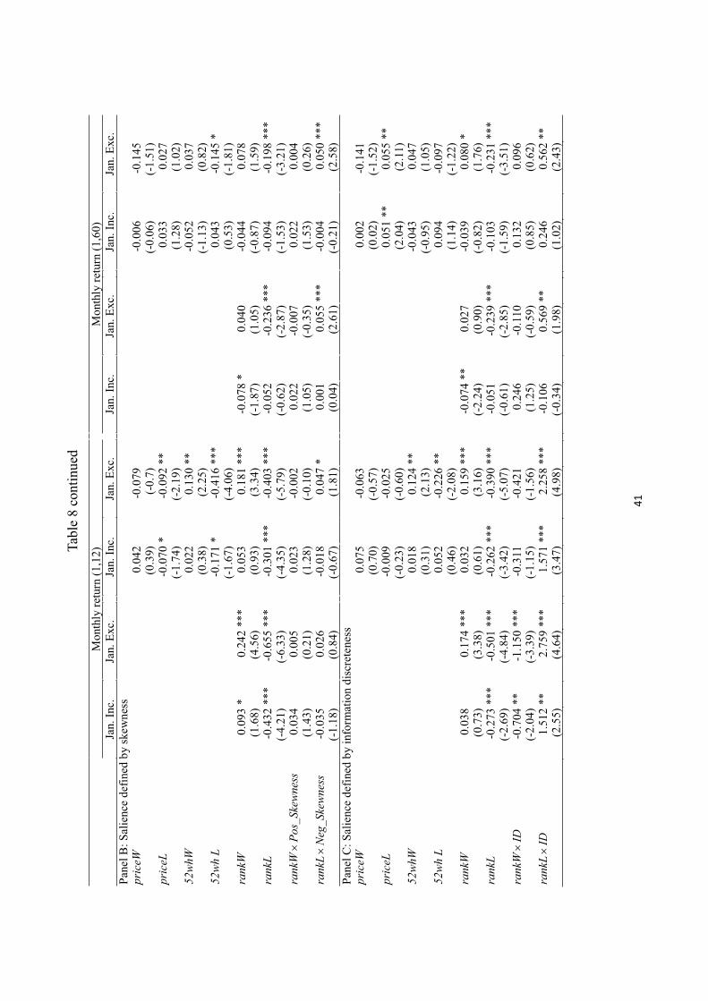
41
Tabl
e 8
cont
inue
dM
onth
ly re
turn
(1,1
2)M
onth
ly re
turn
(1,6
0)Ja
n. In
c.Ja
n. E
xc.
Jan.
Inc.
Jan.
Exc
.Ja
n. In
c.Ja
n. E
xc.
Jan.
Inc.
Jan.
Exc
.Pa
nel B
: Sal
ienc
e de
fined
by sk
ewne
sspr
iceW
0.04
2-0
.079
-0.0
06-0
.145
(0.3
9)(-
0.7)
(-0.
06)
(-1.
51)
pric
eL-0
.070
*-0
.092
**0.
033
0.02
7(-
1.74
)(-
2.19
)(1
.28)
(1.0
2)52
whW
0.02
20.
130
**-0
.052
0.03
7(0
.38)
(2.2
5)(-
1.13
)(0
.82)
52w
hL
-0.1
71*
-0.4
16**
*0.
043
-0.1
45*
(-1.
67)
(-4.
06)
(0.5
3)(-
1.81
)ra
nkW
0.09
3*
0.24
2**
*0.
053
0.18
1**
*-0
.078
*0.
040
-0.0
440.
078
(1.6
8)(4
.56)
(0.9
3)(3
.34)
(-1.
87)
(1.0
5)(-
0.87
)(1
.59)
rank
L-0
.432
***
-0.6
55**
*-0
.301
***
-0.4
03**
*-0
.052
-0.2
36**
*-0
.094
-0.1
98**
*(-
4.21
)(-
6.33
)(-
4.35
)(-
5.79
)(-
0.62
)(-
2.87
)(-
1.53
)(-
3.21
)ra
nkW
Pos_
Skew
ness
0.03
40.
005
0.02
3-0
.002
0.02
2-0
.007
0.02
20.
004
(1.4
3)(0
.21)
(1.2
8)(-
0.10
)(1
.05)
(-0.
35)
(1.5
3)(0
.26)
rank
LN
eg_S
kew
ness
-0.0
350.
026
-0.0
180.
047
*0.
001
0.05
5**
*-0
.004
0.05
0**
*(-
1.18
)(0
.84)
(-0.
67)
(1.8
1)(0
.04)
(2.6
1)(-
0.21
)(2
.58)
Pane
l C: S
alie
nce
defin
edby
info
rmat
ion
disc
rete
ness
pric
eW0.
075
-0.0
630.
002
-0.1
41(0
.70)
(-0.
57)
(0.0
2)(-
1.52
)pr
iceL
-0.0
09-0
.025
0.05
1**
0.05
5**
(-0.
23)
(-0.
60)
(2.0
4)(2
.11)
52w
hW0.
018
0.12
4**
-0.0
430.
047
(0.3
1)(2
.13)
(-0.
95)
(1.0
5)52
wh
L0.
052
-0.2
26**
0.09
4-0
.097
(0.4
6)(-
2.08
)(1
.14)
(-1.
22)
rank
W0.
038
0.17
4**
*0.
032
0.15
9**
*-0
.074
**0.
027
-0.0
390.
080
*(0
.73)
(3.3
8)(0
.61)
(3.1
6)(-
2.24
)(0
.90)
(-0.
82)
(1.7
6)ra
nkL
-0.2
73**
*-0
.501
***
-0.2
62**
*-0
.390
***
-0.0
51-0
.239
***
-0.1
03-0
.231
***
(-2.
69)
(-4.
84)
(-3.
42)
(-5.
07)
(-0.
61)
(-2.
85)
(-1.
59)
(-3.
51)
rank
WID
-0.7
04**
-1.1
50**
*-0
.311
-0.4
210.
246
-0.1
100.
132
0.09
6(-
2.04
)(-
3.39
)(-
1.15
)(-
1.56
)(1
.25)
(-0.
59)
(0.8
5)(0
.62)
rank
LID
1.51
2**
2.75
9**
*1.
571
***
2.25
8**
*-0
.106
0.56
9**
0.24
60.
562
**(2
.55)
(4.6
4)(3
.47)
(4.9
8)(-
0.34
)(1
.98)
(1.0
2)(2
.43)

42
Table 9: Correlations between rank and proxies of arbitrage riskThis table reports the averages of cross-sectional correlations between rank and proxies of arbitrage risk. rank is defined as the average of past 6-month rank measure. From July of each year to June of next year, Ivolatility is the variance of residuals obtained from regressing individual stocks’ daily returns on the value-weighted market index over the past year ending in the previous month with a minimum of 250 trading days; Illiq is the Amihud measure calculated over the past year ending in the previous month; Analyst is defined as the number of analysts following the firm at end of June in the current year, and is set to be zero if a firm is not included in the database; Inst% is defined as the percentage of common stocks owned by institutions at end of June in the current year.
rank Ivolatility Illiq Analyst Inst%rank 1.000 -0.324 -0.044 0.096 0.162Ivolatility 1.000 0.423 -0.292 -0.385Illiq 1.000 -0.117 -0.167Analyst 1.000 0.450Inst% 1.000

43
Tabl
e 10
: Per
form
ance
of N
PMpr
ofits
cond
ition
al o
n ar
bitra
ge ri
skIn
eac
h m
onth
tfr
om Ja
nuar
y 19
63 to
Dec
embe
r 201
5, w
e pe
rfor
m th
e fo
llow
ing
cros
s-se
ctio
nal r
egre
ssio
ns fo
r (j=
1,..
., 12
to j
= 1,
..., 6
0):
,=
,+
,,
+,
,+
,,
+,
,+
,52
,+
,52
,+
,,
+,
,
+,
,,
+,
,,
+,
,w
here
,
is th
e re
turn
of
stoc
k ii
n m
onth
t;,
is th
e na
tura
l log
arith
m o
f st
ock
i’s m
arke
t cap
italiz
atio
n at
the
end
of p
revi
ous
mon
th;
,
(,
),52
,(52
,),
and
,(
,)a
redu
mm
y va
riabl
esth
at e
qual
s 1 if
stoc
k i’s
past
6-m
onth
ave
rage
retu
rn,5
2-w
eek
high
m
easu
re, a
nd p
ast 6
-mon
th ra
nk m
easu
re is
rank
ed a
t the
top
(bot
tom
) 30%
at t
he e
nd o
f mon
th t
j, an
d ze
ro o
ther
wis
e;,
is st
ock
i’sar
bitra
ge ri
sk
mea
sure
cal
cula
ted
in m
onth
tj.
In P
anel
s A to
D, t
he a
rbitr
age
risk
mea
sure
is p
roxi
ed b
y ,
,,
,,
,and
%,
,res
pect
ivel
y.In
eac
h m
onth
t, w
e es
timat
e th
e cr
oss-
sect
iona
l reg
ress
ions
for j
= 1,
..., 1
2 to
j=
1,...
, 60
and
aver
age
the
corr
espo
ndin
g co
effic
ient
est
imat
es. N
umbe
rs in
the
pare
nthe
ses a
re th
e t-s
tatis
tics c
alcu
late
d us
ing
New
ey a
nd W
est’s
(198
7) ro
bust
stan
dard
err
ors.
***,
**,
and
* d
enot
e si
gnifi
canc
e at
the
1%, 5
%, a
nd 1
0% le
vels
, re
spec
tivel
y.M
onth
ly re
turn
(1,1
2)M
onth
ly re
turn
(1,6
0)Ja
n. In
c.Ja
n. E
xc.
Jan.
Inc.
Jan.
Exc
.Ja
n. In
c.Ja
n. E
xc.
Jan.
Inc.
Jan.
Exc
.Pa
nel A
:Ivo
latil
ityas
the
arbi
trage
risk
mea
sure
pric
eW0.
035
-0.0
28-0
.023
-0.1
01(0
.42)
(-0.
31)
(-0.
33)
(-1.
39)
pric
eL-0
.110
***
-0.1
49**
*0.
033
0.00
8(-
2.94
)(-
3.80
)(1
.55)
(0.3
8)52
whW
0.05
80.
143
***
-0.0
270.
036
(1.2
7)(3
.12)
(-0.
79)
(1.0
9)52
wh
L-0
.209
***
-0.3
33**
*0.
002
-0.0
96*
(-2.
82)
(-4.
30)
(0.0
1)(-
1.72
)ra
nkW
0.11
10.
478
***
0.00
80.
297
*-0
.088
0.27
7*
-0.0
690.
245
*(0
.60)
(2.6
0)(0
.05)
(1.8
5)(-
0.52
)(1
.68)
(-0.
46)
(1.6
6)ra
nkL
-0.0
840.
194
0.01
70.
328
***
-0.0
330.
249
**-0
.069
0.22
6**
(-0.
65)
(1.5
0)(0
.15)
(2.8
8)(-
0.30
)(2
.30)
(-0.
70)
(2.3
6)ra
nkW
Ivol
atili
ty0.
020
-0.0
820.
033
-0.0
480.
016
-0.1
050.
018
-0.0
82(0
.29)
(-1.
16)
(0.5
9)(-
0.85
)(0
.23)
(-1.
60)
(0.3
4)(-
1.57
)ra
nkL
Ivol
atili
ty-0
.096
-0.2
48**
*-0
.082
*-0
.220
***
0.00
5-0
.145
***
0.00
8-0
.129
***
(-1.
64)
(-5.
23)
(-1.
67)
(-4.
55)
(0.0
8)(-
3.20
)(0
.16)
(-2.
72)

44
Tabl
e10
con
tinue
dM
onth
ly re
turn
(1,1
2)M
onth
ly re
turn
(1,6
0)Ja
n. In
c.Ja
n. E
xc.
Jan.
Inc.
Jan.
Exc
.Ja
n. In
c.Ja
n. E
xc.
Jan.
Inc.
Jan.
Exc
.Pa
nel B
:Illi
qas
the
arbi
trage
risk
mea
sure
pric
eW0.
024
-0.0
81-0
.065
-0.1
89*
(0.2
2)(-
0.72
)(-
0.69
)(-
1.91
)pr
iceL
-0.0
81*
-0.0
90*
0.04
40.
048
(-1.
86)
(-1.
93)
(1.5
3)(1
.60)
52w
hW0.
049
0.14
6**
*-0
.02
0.06
1(0
.88)
(2.6
0)(-
0.44
)(1
.32)
52w
hL
-0.2
39**
*-0
.418
***
-0.0
18-0
.166
**(-
2.68
)(-
4.54
)(-
0.24
)(-
2.23
)ra
nkW
0.10
3*
0.25
3**
*0.
053
0.19
1**
*-0
.077
*0.
046
-0.0
110.
124
**(1
.76)
(4.4
4)(0
.90)
(3.3
6)(-
1.85
)(1
.20)
(-0.
20)
(2.4
3)ra
nkL
-0.4
87**
*-0
.673
***
-0.3
37**
*-0
.439
***
-0.0
89-0
.255
***
-0.1
31*
-0.2
39**
*(-
4.58
)(-
6.03
)(-
4.29
)(-
5.34
)(-
1.02
)(-
2.89
)(-
1.79
)(-
3.16
)ra
nkW
Illiq
0.01
4-0
.003
0.01
3-0
.003
0.00
8-0
.009
0.00
6-0
.012
(1.5
4)(-
0.34
)(1
.57)
(-0.
37)
(1.1
1)(-
1.31
)(0
.75)
(-1.
55)
rank
LIll
iq0.
028
***
0.00
80.
030
***
0.01
00.
012
-0.0
050.
011
-0.0
05(2
.65)
(0.7
9)(3
.03)
(1.0
7)(1
.56)
(-0.
58)
(1.4
0)(-
0.64
)Pa
nel C
:Ana
lyst
1as
the
arbi
trage
risk
mea
sure
pric
eW0.
054
-0.0
68-0
.005
-0.1
22(0
.38)
(-0.
45)
(-0.
04)
(-0.
99)
pric
eL-0
.095
*-0
.124
**0.
013
-0.0
19(-
1.73
)(-
2.13
)(0
.35)
(-0.
49)
52w
hW0.
058
0.13
3*
0.00
20.
074
(0.7
7)(1
.68)
(0.0
4)(1
.27)
52w
hL
-0.0
85-0
.372
**0.
002
-0.1
97*
(-0.
52)
(-2.
28)
(0.0
2)(-
1.84
)ra
nkW
0.12
50.
257
***
0.06
60.
195
***
0.02
60.
135
**0.
042
0.15
5**
(1.6
1)(3
.08)
(0.9
3)(2
.77)
(0.4
6)(2
.51)
(0.6
2)(2
.25)
rank
L-0
.271
-0.4
36**
-0.1
87*
-0.2
24*
-0.0
47-0
.168
-0.0
64-0
.092
(-1.
53)
(-2.
34)
(-1.
65)
(-1.
86)
(-0.
46)
(-1.
64)
(-0.
72)
(-1.
00)
rank
WAn
alys
t10.
106
-0.0
270.
126
-0.0
07-0
.041
-0.1
50-0
.038
-0.1
39(0
.81)
(-0.
19)
(0.9
6)(-
0.05
)(-
0.36
)(-
1.26
)(-
0.33
)(-
1.14
)ra
nkL
Anal
yst1
-0.2
84-0
.796
***
-0.2
46-0
.723
***
-0.1
51-0
.541
***
-0.1
51-0
.521
***
(-1.
31)
(-3.
72)
(-1.
17)
(-3.
47)
(-0.
88)
(-3.
40)
(-0.
95)
(-3.
30)

45
Tabl
e10
con
tinue
dM
onth
ly re
turn
(1,1
2)M
onth
ly re
turn
(1,6
0)Ja
n. In
c.Ja
n. E
xc.
Jan.
Inc.
Jan.
Exc
.Ja
n. In
c.Ja
n. E
xc.
Jan.
Inc.
Jan.
Exc
.Pa
nel D
:Ins
t%1
as th
e ar
bitra
ge ri
sk m
easu
repr
iceW
-0.0
36-0
.178
-0.0
94-0
.228
*(-
0.26
)(-
1.19
)(-
0.80
)(-
1.86
)pr
iceL
0.00
8-0
.020
0.08
2**
*0.
071
**(0
.16)
(-0.
35)
(2.6
5)(2
.17)
52w
hW0.
081
0.16
9**
0.00
80.
086
(1.0
8)(2
.15)
(0.1
4)(1
.47)
52w
hL
-0.0
12-0
.325
**0.
013
-0.1
90*
(-0.
08)
(-2.
06)
(0.1
1)(-
1.73
)ra
nkW
-0.5
61-0
.496
0.11
3*
0.22
8**
*-0
.138
-0.0
470.
035
0.14
4**
(-0.
82)
(-0.
66)
(1.7
7)(3
.62)
(-1.
12)
(-0.
36)
(0.6
3)(2
.58)
rank
L-1
.033
-1.4
11*
-0.3
43**
*-0
.512
***
-0.2
14-0
.454
***
-0.1
54*
-0.2
95**
*(-
1.48
)(-
1.87
)(-
3.20
)(-
4.72
)(-
1.35
)(-
2.82
)(-
1.68
)(-
3.20
)ra
nkW
Inst
%1
-0.0
24-0
.033
-0.0
50-0
.061
0.02
0-0
.001
-0.0
46-0
.071
(-1.
01)
(-1.
31)
(-1.
08)
(-1.
19)
(0.2
7)(-
0.02
)(-
0.86
)(-
1.22
)ra
nkL
Inst
%1
-0.0
19**
*-0
.026
***
-0.0
28**
-0.0
36**
-0.1
03**
*-0
.122
***
-0.1
27*
-0.1
46*
(-2.
71)
(-3.
55)
(-1.
98)
(-2.
33)
(-2.
84)
(-3.
12)
(-1.
80)
(-1.
92)

46
Appendix A: Variable definitions
These variables are defined as follows. As in FF (1992, 1993), from July of each year to June
of next year,
1. Size is defined as the market value of equity in million dollars at the end of June in the current
year;
2. BM is defined as the ratio of book value of equity at the end of the previous year divided by
market capitalization at the end of the previous year;
3. Ivolatility is the variance of residuals obtained from regressing individual stocks’ daily returns
on the value-weighted market index over the past year ending in the previous month with a
minimum of 250 trading days;
4. Illiq is the average value of daily illiquidity measure over the past year ending in the previous
month, where the daily illiquidity measure is calculated as , , ,/( )i d i d i dR P N with ,i dR
representing the absolute value of stock i’s return on day d, ,i dP representing stock i’s
closing price on day d, and ,i dN representing stock i’s number of shares traded on day d;
5. Analyst is defined as the number of analysts following the firm at end of June in the current
year;
6. Inst% is defined as the percentage of the firm’s common stocks owned by institutions at end
of June in the current year;
7. ID is defined as sign , × %,
%,
, where , is stock i’s cumulative
return from t 12 to t 1; %,
and %,
denote the percentages of days with positive
and negative returns, respectively, over the same period. The sign of , , sign( , ),
equals +1 when , > 0 and -1 when , < 0.

47
The data of Analyst are recorded from the Institutional Brokers’ Estimate System (I/B/E/S)
database for the period from 1980 to 2015. Note that Analyst equals 0 if the stock is not included
in the database, as suggested by Bhushan (1994). The data of Inst% are obtained from the
Spectrum/CDA quarterly database, which is available from 1980 to 2015.

48
Appendix B: Sign momentum strategies
In addition to ranks, we also calculate an alternative nonparametric measure based on signs.
The sign measure, , , is an indicator function which takes the value of 1 if stock i’s
corresponding daily return , is positive, and zero otherwise. The average sign measure in
month t, , ( ), is calculated in a similar way.
We identify several interesting results, which are reported in Table A, and are summarized in
the following.
1. Compared with Table 3, although the profits of the sign momentum are smaller in magnitude
than those of the NPM, they are significant in both short and long terms. In Panel A, the “pure”
sign momentum profit controlling for the price momentum and the 52wh momentum is
0.272% with a t-statistic of 3.78 (which is 0.344% for the NPM) for the first year with January
observations and 0.446% with a t-statistic of 6.32 (which is 0.640% for the NPM) for the first
year without January observations. For the entire 5-year holding period with January excluded,
the profits are 0.204% (t-statistic = 3.01) for the sign momentum versus 0.332% (t-statistic =
2.92) for the NPM. The significance of the positive profits remains when the CRR risk
adjustment is taken into account, as presented in Panel B.
2. The 52wh momentum strategy yields a short-term profit of 0.519% (t-statistic = 2.75) for the
first year in non-January observations, and display no long-term continuation or reversal
patterns. Consistent with Panel B of Table 6, the profitability of the 52wh momentum
disappears under the CRR adjustment.
3. The only difference between Tables 3 and A is the short-term profit of the price momentum.
Recalling from Table 3, the price momentum effect totally disappears when the 52wh
momentum and the NPM are incorporated in the regressions. In Table A, the price losers

49
yields significantly negative returns of -0.096% (t-statistic = -2.43) with January months
included and -0.164% (t-statistic = -3.98) with January months excluded, respectively. This
result suggests that the 52wh momentum and the sign momentum cannot totally eliminate the
price momentum effect. However, consistent with Table 6, Panel B of Table A indicates that
the long-term return reversals of the price momentum can be explained by the CRR five-
factor model. This finding again confirms that long-term return reversals are fully resolved
by the CRR model, and that inclusion of the sign momentum does not account for the reversal
patterns.
Overall, Table A confirms our conjecture that the soundness of the sign momentum is not
special to the nonparametric measure, but is also robust to the sign measure. This evidence
indicates that we need not to rely on a particular nonparametric approach to generate momentum
profits. Nevertheless, we still observe slight difference between the NPM and the sign momentum
in explaining the price momentum effect, suggesting that the information contents behind signs
may be partly distinct from those behind ranks.

50
Tabl
e A: P
erfo
rman
ce o
f pro
fits f
rom
pric
e, 5
2-w
eek
high
,and
sign
mom
entu
mst
rate
gies
In e
ach
mon
th t
from
Janu
ary
1963
to D
ecem
ber 2
015,
we
perf
orm
the
follo
win
g cr
oss-
sect
iona
l reg
ress
ions
for (
j= 1
,...,
12 to
j=
1,...
, 60)
:,=
,+
,,
+,
,+
,,
+,
,+
,52
,+
,52
,+
,,
+,
,+
,,
whe
re
,is
the
retu
rn o
fst
ock
iin
mon
th t;
,is
the
natu
ral l
ogar
ithm
of
stoc
k i’s
mar
ket c
apita
lizat
ion
at th
e en
d of
pre
viou
s m
onth
;,
(,
),52
,(52
,),
and
,(
,)a
redu
mm
y va
riabl
esth
at e
qual
s 1 if
sto
ck i’
spas
t 6-m
onth
ave
rage
retu
rn,5
2-w
eek
high
m
easu
re, a
nd p
ast 6
-mon
th s
ign
mea
sure
is ra
nked
at t
he to
p (b
otto
m) 3
0% a
t the
end
of m
onth
tj,
and
zero
oth
erw
ise.
In e
ach
mon
th t,
we
estim
ate
the
cros
s-se
ctio
nal r
egre
ssio
ns fo
r j=
1,...
, 12
to j
= 1,
..., 6
0an
d av
erag
e th
e co
rres
pond
ing
coef
ficie
nt e
stim
ates
.In
Pane
l A, w
e re
port
the
raw
retu
rn, w
hile
in P
anel
B, w
e pe
rfor
m ti
me-
serie
s re
gres
sion
s of
thes
e av
erag
es (o
ne fo
r eac
h av
erag
e) o
n th
e co
ntem
pora
neou
s C
RR
’sfiv
e fa
ctor
s to
hed
ge o
ut th
e ris
k ex
posu
re.N
umbe
rs in
th
e pa
rent
hese
s ar
e th
e t-s
tatis
tics
calc
ulat
ed u
sing
New
ey a
nd W
est’s
(198
7) ro
bust
sta
ndar
d er
rors
. ***
, **,
and
* d
enot
e si
gnifi
canc
e at
the
1%, 5
%, a
nd 1
0%
leve
ls, r
espe
ctiv
ely.
Mon
thly
retu
rn (1
,12)
Mon
thly
retu
rn (1
3,24
)M
onth
ly re
turn
(25,
36)
Mon
thly
retu
rn (3
7,48
)M
onth
ly re
turn
(1,6
0)Ja
n. In
c.Ja
n. E
xc.
Jan.
Inc.
Jan.
Exc
.Ja
n. In
c.Ja
n. E
xc.
Jan.
Inc.
Jan.
Exc
.Ja
n. In
c.Ja
n. E
xc.
Pane
l A: R
aw re
turn
spr
iceW
0.03
90.
169
**-0
.057
0.06
5-0
.077
0.04
9-0
.058
0.04
7-0
.046
0.06
7(0
.57)
(2.4
5)(-
0.92
)(1
.10)
(-1.
28)
(0.8
4)(-
1.04
)(0
.84)
(-0.
85)
(1.2
5)pr
iceL
-0.0
35-0
.350
***
0.17
4-0
.090
0.14
2-0
.056
0.08
3-0
.096
0.08
2-0
.140
(-0.
27)
(-2.
75)
(1.5
1)(-
0.81
)(1
.37)
(-0.
55)
(0.9
3)(-
1.08
)(0
.86)
(-1.
50)
52w
hW0.
072
-0.0
38-0
.096
-0.2
11**
-0.0
37-0
.162
*0.
022
-0.1
12-0
.004
-0.1
26(0
.69)
(-0.
35)
(-1.
07)
(-2.
17)
(-0.
41)
(-1.
75)
(0.2
5)(-
1.23
)(-
0.04
)(-
1.41
)52
wh
L-0
.096
**-0
.164
***
0.07
7**
0.01
80.
047
0.00
20.
026
0.00
20.
024
-0.0
18(-
2.43
)(-
3.98
)(2
.16)
(0.5
4)(1
.42)
(0.0
6)(0
.81)
(0.0
5)(1
.11)
(-0.
84)
signW
0.08
5**
0.17
4**
*-0
.017
0.07
7*
-0.0
480.
043
-0.0
400.
039
-0.0
230.
063
*(2
.14)
(4.4
5)(-
0.40
)(1
.83)
(-1.
07)
(0.9
8)(-
0.95
)(0
.95)
(-0.
59)
(1.6
9)si
gnL
-0.1
86**
*-0
.273
***
-0.0
40-0
.132
***
-0.0
19-0
.102
**-0
.005
-0.0
71*
-0.0
64*
-0.1
40**
*(-
4.57
)(-
6.79
)(-
0.90
)(-
3.09
)(-
0.42
)(-
2.26
)(-
0.14
)(-
1.85
)(-
1.83
)(-
4.02
)
pric
em
omen
tum
0.16
80.
127
-0.1
73*
-0.2
28**
-0.0
84-0
.164
-0.0
03-0
.113
-0.0
28-0
.109
(1.4
3)(1
.01)
(-1.
76)
(-2.
14)
(-0.
85)
(-1.
63)
(-0.
04)
(-1.
21)
(-0.
32)
(-1.
18)
52w
hm
omen
tum
0.07
40.
519
***
-0.2
310.
155
-0.2
190.
106
-0.1
410.
143
-0.1
280.
207
(0.3
9)(2
.75)
(-1.
35)
(0.9
4)(-
1.38
)(0
.68)
(-1.
02)
(1.0
4)(-
0.87
)(1
.44)
sign
mom
entu
m0.
272
***
0.44
6**
*0.
023
0.20
9**
*-0
.029
0.14
5*
-0.0
340.
110
0.04
10.
204
***
(3.7
8)(6
.32)
(0.2
8)(2
.67)
(-0.
35)
(1.7
8)(-
0.47
)(1
.51)
(0.6
0)(3
.01)

51
Tabl
e Aco
ntin
ued
Mon
thly
retu
rn (1
,12)
Mon
thly
retu
rn (1
3,24
)M
onth
ly re
turn
(25,
36)
Mon
thly
retu
rn (3
7,48
)M
onth
ly re
turn
(1,6
0)Ja
n. In
c.Ja
n. E
xc.
Jan.
Inc.
Jan.
Exc
.Ja
n. In
c.Ja
n. E
xc.
Jan.
Inc.
Jan.
Exc
.Ja
n. In
c.Ja
n. E
xc.
Pane
l B: R
isk-
adju
sted
retu
rns u
sing
the
CR
R fi
ve-f
acto
r ret
urns
pric
eW-0
.084
**-0
.017
0.00
00.
041
0.03
50.
081
*0.
054
0.10
2**
-0.0
010.
049
(-2.
06)
(-0.
41)
(0.0
1)(0
.99)
(0.7
7)(1
.83)
(1.2
1)(2
.40)
(-0.
02)
(1.5
6)pr
iceL
0.02
70.
013
-0.0
16-0
.007
-0.0
34-0
.042
-0.0
06-0
.006
0.00
70.
007
(0.9
6)(0
.46)
(-0.
50)
(-0.
22)
(-1.
15)
(-1.
42)
(-0.
21)
(-0.
18)
(0.4
1)(0
.40)
52w
hW0.
018
-0.0
36-0
.006
-0.0
41-0
.021
-0.0
35-0
.019
-0.0
36-0
.012
-0.0
41*
(0.5
3)(-
1.13
)(-
0.18
)(-
1.34
)(-
0.72
)(-
1.22
)(-
0.64
)(-
1.23
)(-
0.50
)(-
1.91
)52
wh
L0.
054
0.11
3**
*0.
163
***
0.22
8**
*0.
126
***
0.18
0**
*0.
068
0.08
6**
0.08
3**
0.12
4**
*(1
.21)
(2.5
9)(3
.16)
(4.4
8)(2
.67)
(3.7
7)(1
.60)
(1.9
8)(2
.40)
(3.6
3)sig
nW0.
130
***
0.12
1**
*0.
028
0.04
7*
0.03
10.
043
0.04
20.
025
0.04
5**
0.04
1**
(4.7
7)(4
.41)
(1.0
3)(1
.72)
(1.1
5)(1
.57)
(1.6
4)(1
.03)
(2.3
0)(2
.11)
signL
-0.1
72**
*-0
.184
***
-0.0
21-0
.035
-0.0
50*
-0.0
45-0
.023
-0.0
28-0
.070
***
-0.0
72**
*(-
5.42
)(-
6.03
)(-
0.65
)(-
1.13
)(-
1.67
)(-
1.50
)(-
0.78
)(-
0.98
)(-
3.23
)(-
3.42
)
pric
em
omen
tum
-0.1
11*
-0.0
300.
017
0.04
70.
070
0.12
3**
0.06
10.
107
*-0
.008
0.04
2(-
1.94
)(-
0.51
)(0
.27)
(0.7
8)(1
.09)
(1.9
9)(1
.00)
(1.8
5)(-
0.18
)(1
.04)
52w
hm
omen
tum
-0.0
36-0
.149
**-0
.169
**-0
.269
***
-0.1
47**
-0.2
15**
*-0
.087
-0.1
22**
-0.0
95*
-0.1
65**
*(-
0.54
)(-
2.44
)(-
2.36
)(-
3.89
)(-
2.30
)(-
3.35
)(-
1.47
)(-
2.04
)(-
1.83
)(-
3.34
)si
gnm
omen
tum
0.30
2**
*0.
305
***
0.04
80.
082
*0.
082
*0.
088
**0.
066
0.05
40.
115
***
0.11
3**
*(6
.89)
(6.9
3)(1
.05)
(1.8
2)(1
.92)
(2.1
1)(1
.57)
(1.3
8)(3
.81)
(3.8
5)