10. artificial neural networks - chloé...
TRANSCRIPT

10. Artificial Neural Networks
Foundations of Machine LearningÉcole Centrale Paris — Fall 2015
Chloé-Agathe AzencotCentre for Computational Biology, Mines ParisTech
chloeagathe.azencott@minesparistech.fr

2
Learning objectives
● Draw a perceptron and write out its decision function.
● Implement the learning algorithm for a perceptron.● Write out the decision function and weight updates
for any multiple layer perceptron.● Design and train a multiple layer perceptron.

3
The human brain● Networks of processing units (neurons) with
connections (synapses) between them● Large number of neurons: 1010
● Large connectitivity: 104
● Parallel processing● Distributed computation/memory● Robust to noise, failures

4
1950s – 1970s:The perceptron

5
Perceptron[Rosenblatt, 1958]
...INPUT
OUTPUT
Bias unit
Connection weights

6
Perceptron
How can we do classification?
...
[Rosenblatt, 1958]

7
Classification with the perceptron
What is the shape of the decision boundary?
Classification: If f(x) > 0: Positive else Negative
...
threshold function

8
Classification with the perceptron
The decision boundary is a hyperplane (a line in dim 2).Which other methods have we seen that yield decision boundaries that are lines/hyperplanes?
Classification: If f(x) > 0: Positive else Negative
...

9
Classification with the perceptron
What if instead of just a decision (+/-) we want to output the probability of belonging to the positive class?
Classification: If f(x) > 0: Positive else Negative
...

10
Classification with the perceptron
Probability of belonging to the positive class:f(x) = logistic(wTx) = sigmoid(wTx)
...

11
Perceptron: 1D summary● Regression: f(x) = wx + w0
● Classification: f(x) = 1 / (1 + exp -(wx + w0))
ww0
f(x)
xx0=+1
x
w0
o(x)

12
Multiclass classifcationUse K output units
...
...
How do we take a final decision?

13
Multiclass classifcation
● Choose Ck if...
...
● To get probabilities, use the softmax:
– If the output for one class is sufficiently larger than for the others, its softmax will be close to 1 (0 otherwise)
– Similar to the max, but differentiable

14
Training a perceptron

15
Training a perceptron● Online (instances seen one by one) vs batch (whole
sample) learning:– No need to store the whole sample– Problem may change in time– Wear and degradation in system components
16
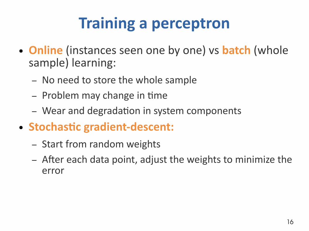
Training a perceptron● Online (instances seen one by one) vs batch (whole
sample) learning:– No need to store the whole sample– Problem may change in time– Wear and degradation in system components
● Stochastic gradient-descent: – Start from random weights– After each data point, adjust the weights to minimize the
error

17
Training a perceptron● Generic update rule:
● After each training instance, for each weight:Learning rate
wj
E(wj)

18
Training a perceptron: regression
● Regression
● What is the update rule?

19
Training a perceptron: regression
● Regression
● The update rule for the regression is:

20
y = 1 y = 0
f(x) f(x)
Erro
r
Erro
r
Training a perceptron: classification● Sigmoid output:
● Cross-entropy error:
● What is the update rule now?

21
y = 1 y = 0
f(x)Er
ror
Training a perceptron: classification● Sigmoid output:
● Cross-entropy error:
● Update rule for binary classification:
f(x)
Erro
r

22
Training a perceptron: K classes
● K > 2 softmax outputs:
● Cross-entropy error:
● Update rule for K-way classification:
23
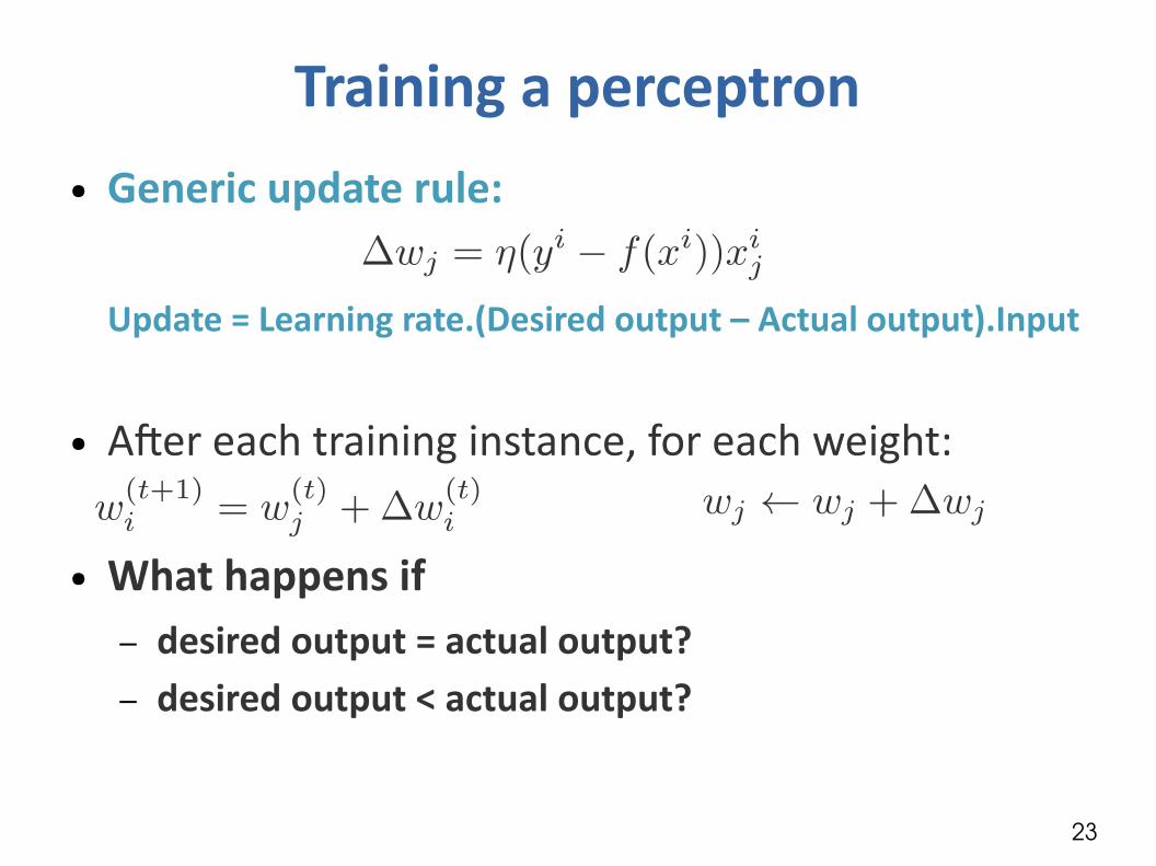
Training a perceptron● Generic update rule:
Update = Learning rate.(Desired output – Actual output).Input
● After each training instance, for each weight:
● What happens if – desired output = actual output?– desired output < actual output?

24
● Generic update rule:
Update = Learning rate.(Desired output – Actual output).Input
● After each training instance, for each weight:
– If desired output = actual output: no change– If desired output < actual output:
● input > 0 → update < 0 → smaller → prediction ↘● input < 0 → update > 0 → smaller → prediction ↘
Training a perceptron: regression

25
Learning boolean functions

26
Learning ANDx1 x2 y0 0 00 1 01 0 01 1 1
Design a perceptron that learns AND.– What is its architecture?

27
Learning ANDx1 x2 y0 0 00 1 01 0 01 1 1
Design a perceptron that learns AND.
Draw the 4 possible points (x1, x2) and a desirable separating line. What is its equation?

28
Learning ANDx1 x2 y0 0 00 1 01 0 01 1 1
Design a perceptron that learns AND.
29
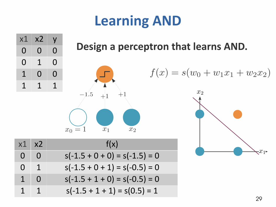
Learning ANDx1 x2 y0 0 00 1 01 0 01 1 1
Design a perceptron that learns AND.
x1 x2 f(x)0 0 s(-1.5 + 0 + 0) = s(-1.5) = 00 1 s(-1.5 + 0 + 1) = s(-0.5) = 01 0 s(-1.5 + 1 + 0) = s(-0.5) = 01 1 s(-1.5 + 1 + 1) = s(0.5) = 1

30
Learning XORDesign a perceptron that learns XORx1 x2 y
0 0 00 1 11 0 11 1 0
31
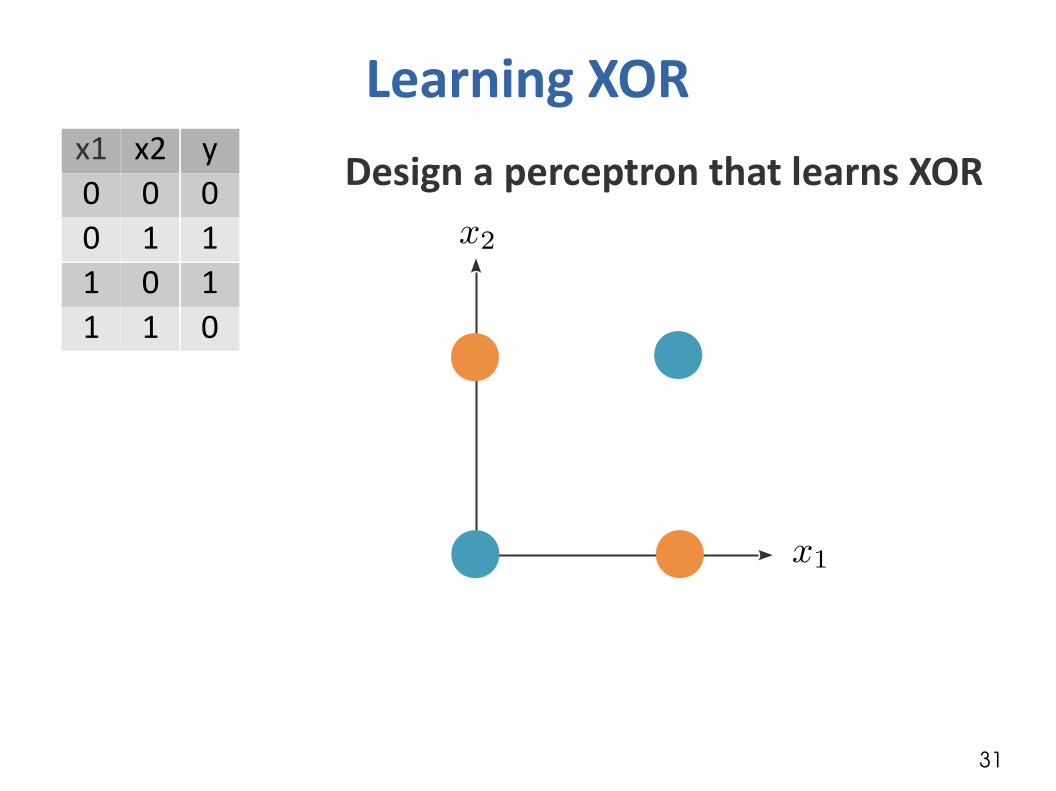
Learning XORDesign a perceptron that learns XORx1 x2 y
0 0 00 1 11 0 11 1 0

32
Learning XOR
[Minsky and Papert, 1969]
No w0, w1, w2 satisfy:
x1 x2 y0 0 00 1 11 0 11 1 0

33
Perceptrons
The perceptron has shown itself worthy of study despite (and even because of!) its severe limitations. It has many features to attract attention: its linearity; its intriguing learning theorem; its clear paradigmatic simplicity as a kind of parallel computation. There is no reason to suppose that any of these virtues carry over to the many-layered version. Nevertheless, we consider it to be an important research problem to elucidate (or reject) our intuitive judgement that the extension to multilayer systems is sterile.
M. Minsky & S. Papert, 1969

34
1980s – early 1990s

35
Multilayer perceptrons
...
... Hidden layer
Write the prediction f(x).

36
Multilayer perceptrons
...
...
● Output of hidden unit (h):
● Output of the network:
Not linear in x!

37
Learning XOR with an MLP
Draw the geometric interpretation of this multiple layer perceptron.

38
Learning XOR with an MLP

39
Universal approximationAny continuous function on a compact subset of can be approximated to any arbitrary degree of precision by a feed-forward multi-layer perceptron with a single hidden layer containing a finite number of neurons.
Cybenko (1989), Hornik (1991)
40
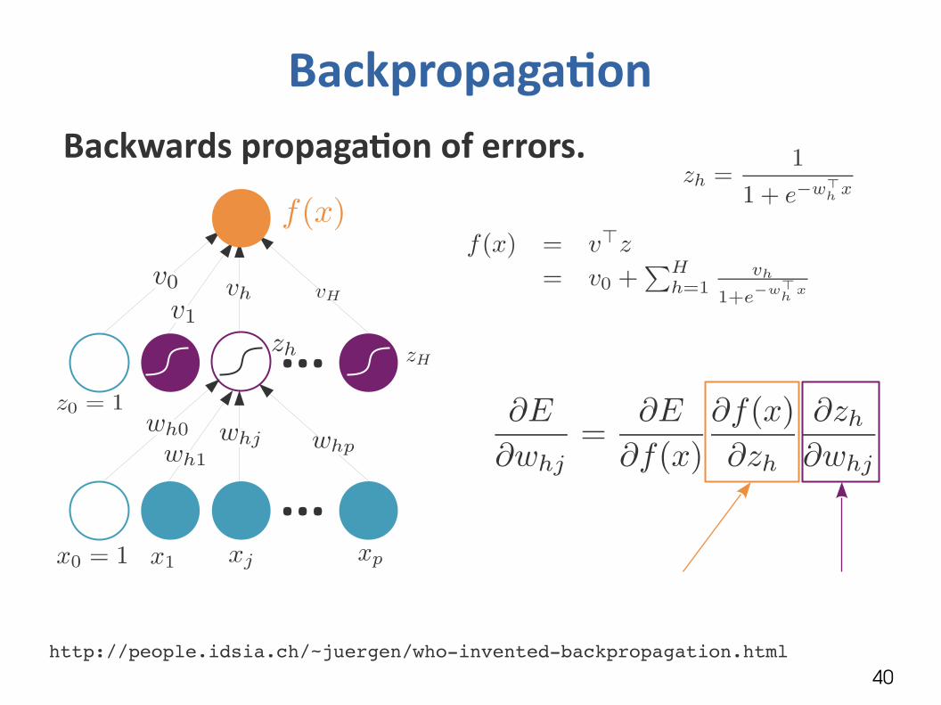
Backpropagation
...
...
Backwards propagation of errors.
http://people.idsia.ch/~juergen/whoinventedbackpropagation.html

41
Backpropagation
...
...
Backwards propagation of errors.

42
Backprop: Regression
ForwardBackward

43
Backprop: Regression
...
...

44
Backprop: Regression
...
...
Epoch: when all the training points have been seen once

45
E.g.: Learning sin(x)
Source: Ethem Alpaydin
training
validation
training points
sin(x)
learned curve(200 epochs)
# epochs
Mea
n Sq
uare
Err
or
46
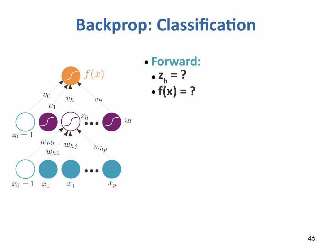
Backprop: Classification
...
...
● Forward:● zh = ?● f(x) = ?
47
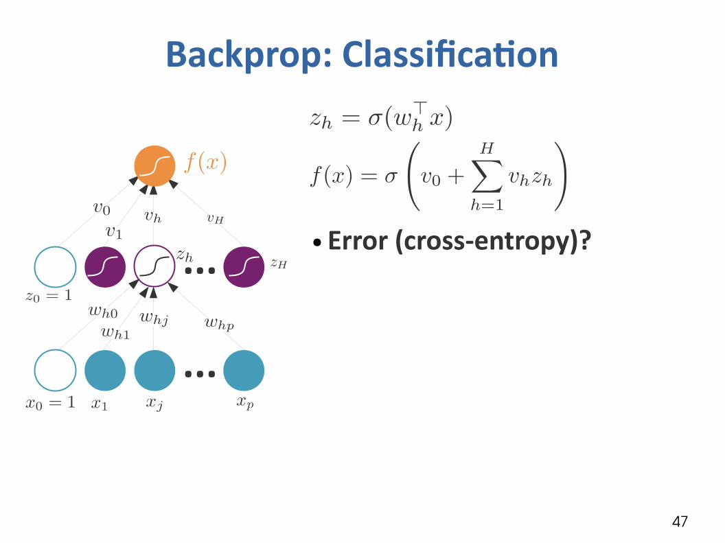
Backprop: Classification
...
...● Error (cross-entropy)?
48
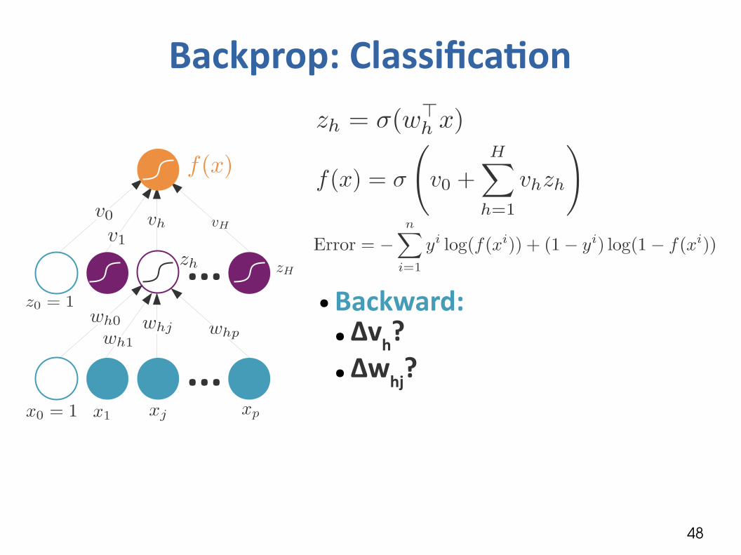
Backprop: Classification
...
...● Backward:
● Δvh?● Δwhj?

49
Backprop: Classification
...
...

50
Backprop: K classes

51
Multiple hidden layers● The MLP with one hidden layer is a universal approximator ● But using multiple layers may lead to simpler networks.
...
...
...
52
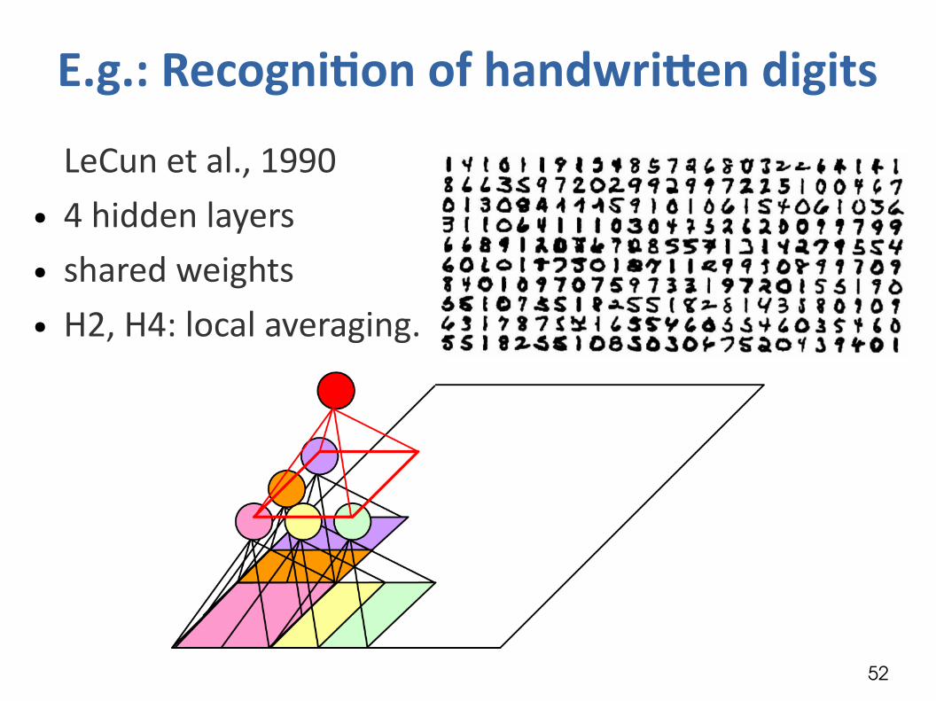
E.g.: Recognition of handwriten digits
LeCun et al., 1990● 4 hidden layers● shared weights● H2, H4: local averaging.

53
Neural networks packages● Matlab
– Neural Network Toolbox– Deep Learn Toolbox, Deep Belief Networks, and others at
http://deeplearning.net/software_links/● Python
– bpnn.py– fnnet– (C bindings) FANN– PyNN– PyAnn– nnutils based on Monte– theano
● R– neuralnet– nnet

54
Summary● Perceptrons learn linear discriminants.● Learning is done by weight update.● Multiple layer perceptrons with one hidden unit are
universal approximators.● Learning is done by backpropagation.● Neural networks are hard to train, caution must be
applied.

55
References● Le Cun, Y., Bengio, Y. and Hinton, G. (2015). Deep
learning. Nature 521, 436-444.