10: carrierrecovery carrierrecoverysunar/courses/ece3311/slides/ch10.pdf · 10: carrierrecovery...
TRANSCRIPT
10: Carrier Recovery
CARRIER RECOVERY
⋆ Phase Tracking
◦ Squared Difference◦ Phase-locked Loop◦ Costas Loop◦ Decision Directed
⋆ Frequency Tracking
adaptive components
Software Receiver Design Johnson/Sethares/Klein 1 / 45
10: Carrier Recovery
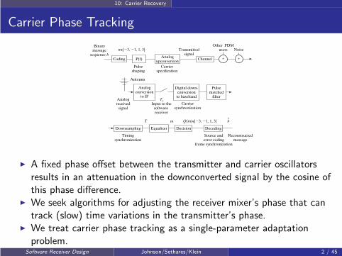
Carrier Phase Tracking
Transmitted signal
we{23, 21, 1, 3}
Coding
Pulse shaping
Analog upconversion
Channel
NoiseOther FDM
users
P(f)
Analog conversion
to IF
Digital down- conversion
to baseband
EqualizerDownsampling Decision Decoding
Ts Input to the
software receiver
Timing synchronization
T
Analog received
signal
Reconstructed message
Source and error coding
frame synchronization
Q(m)e{23, 21, 1, 3}
Carrier synchronization
Antenna
Carrier specification
Binary message
sequence b
m b^
Pulse matched
filter
1 1
◮ A fixed phase offset between the transmitter and carrier oscillatorsresults in an attenuation in the downconverted signal by the cosine ofthis phase difference.
◮ We seek algorithms for adjusting the receiver mixer’s phase that cantrack (slow) time variations in the transmitter’s phase.
◮ We treat carrier phase tracking as a single-parameter adaptationproblem.
Software Receiver Design Johnson/Sethares/Klein 2 / 45
10: Carrier Recovery
Adaptive Algorithm Development
Our (single-parameter) adaptive algorithm development strategy:
1. Propose a cost function assessing behavior over measured data set.
2. Check location of minima and maxima in terms of adjusted parameterto see if in desired location.
3. Pursue (small stepsize) gradient descent strategy (with itscommutability of averaging and differentiation). The correction termmust be calculable from available signals.
4. Test performance.
Software Receiver Design Johnson/Sethares/Klein 3 / 45
10: Carrier Recovery
Phase Tracking
Carrier extraction
◮ For AM with large carrier, we could narrowly BPF the received signalto extract (mostly) just the carrier and then use a Fourier Transformor build a simpler sinusoid tracker that finds the carrier signal’s phase.
◮ For AM with suppressed carrier we have to process the receivedupconverted signal
r(t) = s(t)cos(2πfct+ φ)
which does not include an additive carrier.
◮ Consider squaring the received signal and using (A.4) to produce
r2(t) = (1/2)s2(t)[1 + cos(4πfct+ 2φ)]
Software Receiver Design Johnson/Sethares/Klein 4 / 45
10: Carrier Recovery
Phase Tracking (cont’d)
Carrier extraction (cont’d)
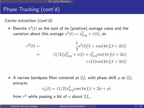
◮ Rewrite s2(t) as the sum of its (positive) average value and thevariation about this average s2(t) = s2avg + v(t), so
r2(t) =1
2s2(t)[1 + cos(4πfct+ 2φ)]
= (1/2)[s2avg + v(t) + s2avgcos(4πfct+ 2φ)
+v(t)cos(4πfct+ 2φ)]
◮ A narrow bandpass filter centered at 2fc with phase shift ρ at 2fcextracts
rp(t) = (1/2)s2avgcos(4πfct+ 2φ+ ρ)
from r2 while passing a bit of v about 2fc.
Software Receiver Design Johnson/Sethares/Klein 5 / 45
10: Carrier Recovery
Phase Tracking (cont’d)
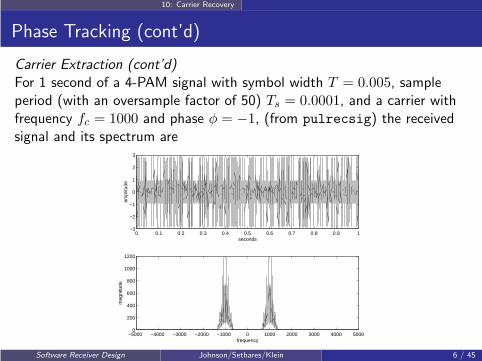
Carrier Extraction (cont’d)For 1 second of a 4-PAM signal with symbol width T = 0.005, sampleperiod (with an oversample factor of 50) Ts = 0.0001, and a carrier withfrequency fc = 1000 and phase φ = −1, (from pulrecsig) the receivedsignal and its spectrum are
0 0.1 0.2 0.3 0.4 0.5 0.6 0.7 0.8 0.9 1−3
−2
−1
0
1
2
3
seconds
ampl
itude
−5000 −4000 −3000 −2000 −1000 0 1000 2000 3000 4000 50000
200
400
600
800
1000
1200
frequency
mag
nitu
de
Software Receiver Design Johnson/Sethares/Klein 6 / 45
10: Carrier Recovery
Phase Tracking (cont’d)
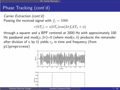
Carrier Extraction (cont’d)Passing the received signal with fc = 1000
r(kTs) = s(kTs)cos(2πfckTs + φ)
through a squarer and a BPF centered at 2000 Hz with approximately 100Hz passband and mod(ρ, 2π)=0 (where mod(a, b) produces the remainderafter division of a by b) yields rp in time and frequency (frompllpreprocess)
0 0.1 0.2 0.3 0.4 0.5 0.6 0.7 0.8 0.9 1−2
−1
0
1
2
seconds
ampl
itude
−5000 −4000 −3000 −2000 −1000 0 1000 2000 3000 4000 50000
1000
2000
3000
4000
5000
frequency
mag
nitu
de
Software Receiver Design Johnson/Sethares/Klein 7 / 45
10: Carrier Recovery
Phase Tracking (cont’d)
Squared DifferenceWe have extracted from the received PAM signal a signal
rp(kTs) ≈ (1/2)s2avgcos(4πfckTs + 2φ+ ρ)
that crudely approximates a cosine with twice the frequency and phase ofthe carrier. Assume we generate a local sinusoid of frequency f0 = fc andselect θ in
cos(4πf0kTs + 2θ +mod(ρ, 2π))
to attempt to match rp by minimizing
JSD =1
4P
P∑
k=1
[2
s2avgrp(kTs)− cos(4πf0kTs + 2θ +mod(ρ, 2π))]2
=1
4avg{[
2
s2avgrp(kTs)− cos(4πf0kTs + 2θ +mod(ρ, 2π))]2}
which should happen at θ = φ for a well-extracted cosine in rp.Software Receiver Design Johnson/Sethares/Klein 8 / 45
10: Carrier Recovery
Phase Tracking (cont’d)
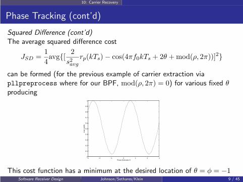
Squared Difference (cont’d)The average squared difference cost
JSD =1
4avg{[
2
s2avgrp(kTs)− cos(4πf0kTs + 2θ +mod(ρ, 2π))]2}
can be formed (for the previous example of carrier extraction viapllpreprocess where for our BPF, mod(ρ, 2π) = 0) for various fixed θproducing
−3 −2 −1 0 1 2 30
0.1
0.2
0.3
0.4
0.5
0.6
0.7
0.8
0.9
1
Phase Estimates θ
Cos
t Jsd
(θ)
This cost function has a minimum at the desired location of θ = φ = −1and at locations an integer multiple of π away.Software Receiver Design Johnson/Sethares/Klein 9 / 45

10: Carrier Recovery
Phase Tracking (cont’d)
Squared Difference (cont’d)We will now analytically examine the average squared difference cost JSDwith ψ = mod(ρ, 2π)
JSD = 14avg
{
(
2s2avg
rp(kTs)− cos(4πf0kTs + 2θ + ψ))2
}
◮ First we presume that (2/s2avg)rp is very nearly the carrier at doublefrequency and with double phase plus BPF phase shift ρ withψ = mod(ρ, 2π)
cos(4πf0kTs + 2φ+ ψ)
◮ Second, we note (see Appendix G) that the averaging operation(avg ∼ (1/P )
∑Pk=1) is a lowpass filter with impulse response
{1/P, 1/P, ..., 1/P}.◮ Thus,
JSD(θ) ≈1
4LPF{(cos(4πf0kTs+2φ+ψ)−cos(4πf0kTs+2θ+ψ))2}
Software Receiver Design Johnson/Sethares/Klein 10 / 45

10: Carrier Recovery
Phase Tracking (cont’d)
Squared Difference (cont’d)
◮ Expanding the square yields
JSD(θ) ≈1
2LPF
{
cos2(4πf0kTs + 2φ+ ψ)
−2 cos(4πf0kTs + 2φ+ ψ) cos(4πf0kTs + 2θ + ψ)
+ cos2(4πf0kTs + 2θ + ψ)}
◮ Using (A.4) cos2(x) = 12(1 + cos(2x)) and (A.9)
cos(x)cos(y) =1
2[cos(x− y) + cos(x+ y)]
the cost function becomes
JSD(θ) ≈1
8LPF
{
2 + cos(8πf0kTs + 4φ+ 2ψ)
−2 cos(2φ− 2θ)− 2 cos(8πf0kTs + 2φ+ 2θ + 2ψ)
+ cos(8πf0kTs + 4θ + 2ψ)}
Software Receiver Design Johnson/Sethares/Klein 11 / 45
10: Carrier Recovery
Phase Tracking (cont’d)
Squared Difference (cont’d)
◮ With the linearity of the LPF (so the LPF of the sum is the sum ofthe LPFs of each summand) and the cutoff frequency of the LPF lessthan 4f0 (which, for the averaging operation in JSD, can be madelower for larger P )
JSD(θ) ≈1
4(1− cos(2φ− 2θ))
◮ For a fixed φ a full period ranging in amplitude from approximately 0to 1 is traversed every π along the θ axis by the numerically generatedcost function in agreement with this functional form of JSD.
Software Receiver Design Johnson/Sethares/Klein 12 / 45
10: Carrier Recovery
Phase Tracking (cont’d)
Squared Difference (cont’d)
◮ Our next step in our adaptive algorithm development strategy is toform the gradient of the cost
∂∂θ[14avg{(
2s2avg
rp(kTs)− cos(4πf0kTs + 2θ + ψ))2}]|θ=θ[k]
◮ From Appendix G, we can commute the differentiation and averagingand perform the averaging operation with a LPF with cutoff less than4f0
∼ LPF{ ∂∂θ[14(
2s2avg
rp(kTs)− cos(4πf0kTs + 2θ + ψ))2]|θ=θ[k]}
and retain an accurate approximation of the gradient for a smallstepsize update.
Software Receiver Design Johnson/Sethares/Klein 13 / 45
10: Carrier Recovery
Phase Tracking (cont’d)
Squared Difference (cont’d)
◮ Using (A.59) and (A.60), the partial derivative with respect to θinside the average can be evaluated as
(
2
s2avgrp(kTS)− cos(4πf0kTs + 2θ[k] + ψ)
)
· sin(4πf0kTs+2θ[k]+ψ)
◮ We will assume that 2/s2avg and ψ are known (or computed) at thereceiver.
◮ The resulting squared difference carrier phase tracking algorithm is
θ[k + 1] = θ[k]− µ · LPF{( 2
s2avgrp(kTs)
− cos(4πf0kTs + 2θ[k] + ψ))
sin(4πf0kTs + 2θ[k] + ψ)}
Software Receiver Design Johnson/Sethares/Klein 14 / 45
10: Carrier Recovery
Phase Tracking (cont’d)
Squared Difference (cont’d)
◮ The signal rp is the output of the squarer and narrow BPFcombination with ψ = mod(ρ, 2π) where ρ is the phase of thepreprocessing BPF at 2fc.
◮ In our example, the average s2 can be calculated (in advance) fromthe average squared sample from a single pulse shape (which forhamming(50) is 0.3896) times the averaged squared source symbol(which is 5 for equally likely 4-PAM symbols of ±1s and ±3s) ⇒s2avg ≈ 2 ⇒ 2/s2avg ≈ 1.
◮ Or an AGC can be used to scale rp to be a unit amplitude sinusoid.
Software Receiver Design Johnson/Sethares/Klein 15 / 45
10: Carrier Recovery
Phase Tracking (cont’d)
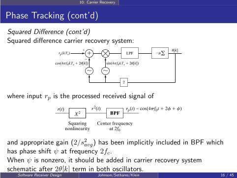
Squared Difference (cont’d)Squared difference carrier recovery system:
LPF
2
2ma
sin(4pf0kTs 1 2u[k])cos(4pf0kTs 1 2u[k])
u[k]1
1
2
rp(kTs)
, ,
where input rp is the processed received signal of
X2 BPFr(t) r2(t)
Squaring nonlinearity
Center frequency at 2f0
rp(t) ~ cos(4pf0t 1 2f 1 c)
and appropriate gain (2/s2avg) has been implicitly included in BPF whichhas phase shift ψ at frequency 2fc.When ψ is nonzero, it should be added in carrier recovery systemschematic after 2θ[k] term in both oscillators.
Software Receiver Design Johnson/Sethares/Klein 16 / 45
10: Carrier Recovery
Phase Tracking (cont’d)
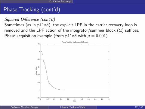
Squared Difference (cont’d)Sometimes (as in pllsd), the explicit LPF in the carrier recovery loop isremoved and the LPF action of the integrator/summer block (Σ) suffices.Phase acquisition example (from pllsd with µ = 0.001)
0 0.2 0.4 0.6 0.8 1 1.2 1.4 1.6 1.8 2−1.2
−1
−0.8
−0.6
−0.4
−0.2
0
0.2Phase Tracking via Squared Difference
time
phas
e of
fset
Software Receiver Design Johnson/Sethares/Klein 17 / 45

10: Carrier Recovery
Phase Tracking (cont’d)
Phase-locked Loop (PLL)To introduce a phase-locked loop, the most widely known carrier recoveryscheme, we present a candidate cost function producing the PLL.
◮ Reconsider the output of the squarer and narrow BPF, which is ascaled version of the carrier rp(kTs) ≈ g cos(4πf0kTs + 2φ+ ψ)where g is s2avg/2 times the square of the product of the channel andBPF gains at 2f0, and ψ is the BPF phase (mod 2π) at 2f0.
◮ Consider downconverting rp(kTs) with our (unsynchronized) receiveroscillator’s output and formrp(kTs) cos(4πf0kTs + 2θ + ψ)
≈ g cos(4πf0kTs + 2φ+ ψ) cos(4πf0kTs + 2θ + ψ)
=g
2{cos(2φ− 2θ) + cos(8πf0kTs + 2φ+ 2θ + 2ψ)}
Software Receiver Design Johnson/Sethares/Klein 18 / 45
10: Carrier Recovery
Phase Tracking (cont’d)
Phase-locked Loop (PLL)
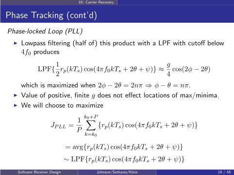
◮ Lowpass filtering (half of) this product with a LPF with cutoff below4f0 produces
LPF{1
2rp(kTs) cos(4πf0kTs + 2θ + ψ)} ≈
g
4cos(2φ− 2θ)
which is maximized when 2φ− 2θ = 2nπ ⇒ φ− θ = nπ.
◮ Value of positive, finite g does not effect locations of max/minima.
◮ We will choose to maximize
JPLL =1
P
k0+P∑
k=k0
{rp(kTs) cos(4πf0kTs + 2θ + ψ)}
= avg{rp(kTs) cos(4πf0kTs + 2θ + ψ)}
∼ LPF{rp(kTs) cos(4πf0kTs + 2θ + ψ)}
Software Receiver Design Johnson/Sethares/Klein 19 / 45

10: Carrier Recovery
Phase Tracking (cont’d)
PLL (cont’d)As a numerical test for extrema, the PLL cost
JPLL = LPF{rp(kTs)cos(4πf0kTs + 2θ + ψ)}
can be formed for various fixed θ producing (via pllconverge)
−3 −2 −1 0 1 2 3−0.5
−0.4
−0.3
−0.2
−0.1
0
0.1
0.2
0.3
0.4
0.5
Phase Estimates θ
Cos
t Jpl
l(θ)
A maximum (near 0.5 with g ≈ 1 in this case) appears at the desiredlocation of θ = φ = −1 (with ψ = 0) and at locations an integer multipleof π away, as predicted in the preceding analysis.
Software Receiver Design Johnson/Sethares/Klein 20 / 45
10: Carrier Recovery
Phase Tracking (cont’d)
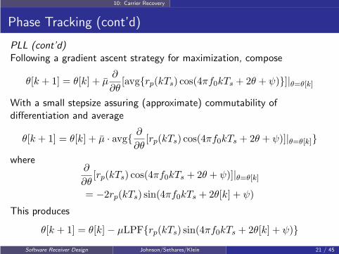
PLL (cont’d)Following a gradient ascent strategy for maximization, compose
θ[k + 1] = θ[k] + µ̄∂
∂θ[avg{rp(kTs) cos(4πf0kTs + 2θ + ψ)}]|θ=θ[k]
With a small stepsize assuring (approximate) commutability ofdifferentiation and average
θ[k + 1] = θ[k] + µ̄ · avg{∂
∂θ[rp(kTs) cos(4πf0kTs + 2θ + ψ)]|θ=θ[k]}
where∂
∂θ[rp(kTs) cos(4πf0kTs + 2θ + ψ)]|θ=θ[k]
= −2rp(kTs) sin(4πf0kTs + 2θ[k] + ψ)
This produces
θ[k + 1] = θ[k]− µLPF{rp(kTs) sin(4πf0kTs + 2θ[k] + ψ)}
Software Receiver Design Johnson/Sethares/Klein 21 / 45
10: Carrier Recovery
Phase Tracking (cont’d)
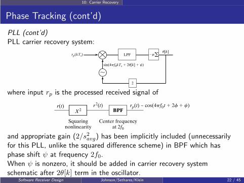
PLL (cont’d)PLL carrier recovery system:
LPF
2
2ma
sin(4pf0kTs 1 2u[k] 1 c)
u[k]rp(kTs)
,
where input rp is the processed received signal of
X2 BPFr(t) r2(t)
Squaring nonlinearity
Center frequency at 2f0
rp(t) ~ cos(4pf0t 1 2f 1 c)
and appropriate gain (2/s2avg) has been implicitly included (unnecessarilyfor this PLL, unlike the squared difference scheme) in BPF which hasphase shift ψ at frequency 2f0.When ψ is nonzero, it should be added in carrier recovery systemschematic after 2θ[k] term in the oscillator.
Software Receiver Design Johnson/Sethares/Klein 22 / 45
10: Carrier Recovery
Phase Tracking (cont’d)
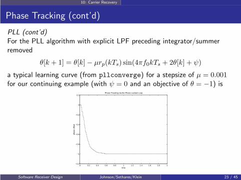
PLL (cont’d)For the PLL algorithm with explicit LPF preceding integrator/summerremoved
θ[k + 1] = θ[k]− µrp(kTs) sin(4πf0kTs + 2θ[k] + ψ)
a typical learning curve (from pllconverge) for a stepsize of µ = 0.001for our continuing example (with ψ = 0 and an objective of θ = −1) is
0 0.2 0.4 0.6 0.8 1 1.2 1.4 1.6 1.8 2−1.2
−1
−0.8
−0.6
−0.4
−0.2
0
0.2Phase Tracking via the Phase Locked Loop
time
phas
e of
fset
Software Receiver Design Johnson/Sethares/Klein 23 / 45
10: Carrier Recovery
Phase Tracking (cont’d)
Costas LoopNow, we seek an algorithm not based on a presumption of carrierextraction from the received signal.
◮ Reconsider the received signal
r(kTs) = s(kTs) cos(2πfckTs + φ).
◮ Assume the transmitter carrier frequency fc and receiver frequencyare identical (fc = f0) and form
2r(kTs) cos(2πf0kTs + θ)
= s(kTs)[cos(φ− θ) + cos(4πf0kTs + φ+ θ)]
◮ With a LPF cutoff below 2f0
LPF{2r(kTs) cos(2πf0kTs + θ)} = v(kTs) cos(φ− θ)
where v(kTs) = LPF{s(kTs)}. If the cutoff frequency of the LPF isabove the bandwidth of the baseband waveform s, then v is s.
Software Receiver Design Johnson/Sethares/Klein 24 / 45
10: Carrier Recovery
Phase Tracking (cont’d)
Costas Loop (cont’d)
◮ As a cost function, consider
JC(θ) =1
P
k0∑
k=k0−(P−1)
{LPF[2r(kTs) cos(2πf0kTs + θ)]}2
≈ avg{v2(kTs) cos2(φ− θ)}
◮ Because the squared cosine term is fixed, given (A.4)
avg{v2(kTs) cos2(φ− θ)}
=(
avg{v2(kTs)}) (1 + cos(2(φ− θ)))
2and assuming that the average of v2 is fixed, this cost function will bemaximized with a value equal to the average of v2 (which is averagevalue of {LPF[s]}2) at φ− θ = πn or θ = φ+ πn for all (positiveand negative) integers n.
Software Receiver Design Johnson/Sethares/Klein 25 / 45
10: Carrier Recovery
Phase Tracking (cont’d)
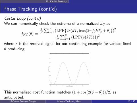
Costas Loop (cont’d)We can numerically check the extrema of a normalized JC as
JNC(θ) =1P
∑Pk=1 (LPF{2r(kTs)cos(2πf0kTs + θ)})2
1P
∑Pk=1 (LPF{s(kTs)})
2
where r is the received signal for our continuing example for various fixedθ producing
−3 −2 −1 0 1 2 30
0.2
0.4
0.6
0.8
1
1.2
1.4
Phase Estimates θ
Cos
t Jnc
(θ)
This normalized cost function matches (1 + cos(2(φ− θ)))/2, asanticipated.
Software Receiver Design Johnson/Sethares/Klein 26 / 45
10: Carrier Recovery
Phase Tracking (cont’d)
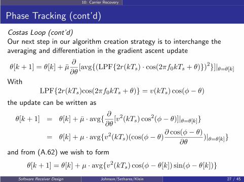
Costas Loop (cont’d)Our next step in our algorithm creation strategy is to interchange theaveraging and differentiation in the gradient ascent update
θ[k + 1] = θ[k] + µ̄∂
∂θ[avg{(LPF{2r(kTs) · cos(2πf0kTs + θ)})2}]|θ=θ[k]
WithLPF{2r(kTs)cos(2πf0kTs + θ)} = v(kTs) cos(φ− θ)
the update can be written as
θ[k + 1] = θ[k] + µ̄ · avg{∂
∂θ[v2(kTs) cos
2(φ− θ)]|θ=θ[k]}
= θ[k] + µ · avg{v2(kTs)(cos(φ− θ)∂ cos(φ− θ)
∂θ)|θ=θ[k]}
and from (A.62) we wish to form
θ[k + 1] = θ[k] + µ · avg{v2(kTs) cos(φ− θ[k]) sin(φ− θ[k])}
Software Receiver Design Johnson/Sethares/Klein 27 / 45

10: Carrier Recovery
Phase Tracking (cont’d)
Costas Loop (cont’d)
◮ Given
LPF{2r(kTs)cos(2πf0kTs + θ)} = v(kTs) cos(φ− θ)
to compose the update from measurable signals we need to find arealizable expression for v(kTs) sin(φ− θ).
◮ For a LPF with cutoff under 2f0, defining v = LPF{s} and using(A.10) and (A.11) producesLPF{2r(kTs) sin(2πf0kTs + θ)}
= LPF{s(kTs) cos(2πf0kTs + φ) sin(2πf0kTs + θ)}
= LPF{s(kTs)(sin(θ − φ)− sin(4πf0kTs + φ+ θ))}
= −v(kTs) sin(φ− θ)
Software Receiver Design Johnson/Sethares/Klein 28 / 45

10: Carrier Recovery
Phase Tracking (cont’d)
Costas Loop (cont’d)Thus, a small stepsize gradient ascent algorithm (for maximization of JC)is
θ[k + 1] = θ[k]− µ · avg[
LPF{2r(kTs) cos(2πf0kTs + θ[k])}
·LPF{2r(kTs) sin(2πf0kTs + θ[k])}]
◮ The use of lowpass filtering in the update is predicated on apresumption that the LPF output is characterized by its asymptoticresponse.
◮ This effectively presumes θ[k] remains fixed for a sufficiently long timefor this asymptotic behavior to be achieved.
◮ We rely on a small stepsize µ to keep θ[k] variations modest in the(relatively) short time frame anticipated for LPF achievement ofasymptotic behavior.
Software Receiver Design Johnson/Sethares/Klein 29 / 45
10: Carrier Recovery
Phase Tracking (cont’d)
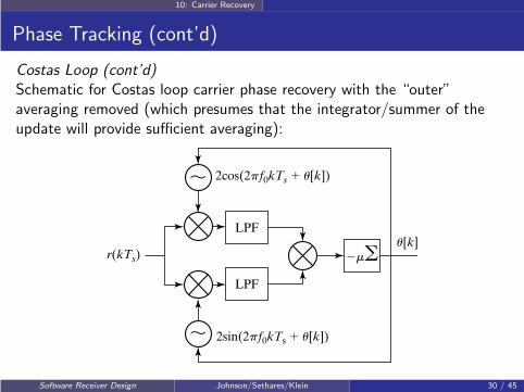
Costas Loop (cont’d)Schematic for Costas loop carrier phase recovery with the “outer”averaging removed (which presumes that the integrator/summer of theupdate will provide sufficient averaging):
2mau[k]
LPF
2cos(2pf0kTs 1 u[k])
2sin(2pf0kTs 1 u[k])
r(kTs)
,
,
LPF
Software Receiver Design Johnson/Sethares/Klein 30 / 45
10: Carrier Recovery
Phase Tracking (cont’d)
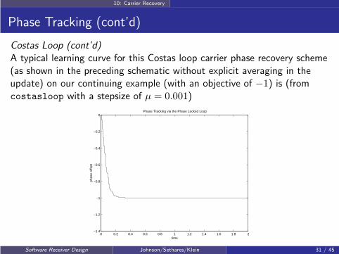
Costas Loop (cont’d)A typical learning curve for this Costas loop carrier phase recovery scheme(as shown in the preceding schematic without explicit averaging in theupdate) on our continuing example (with an objective of −1) is (fromcostasloop with a stepsize of µ = 0.001)
0 0.2 0.4 0.6 0.8 1 1.2 1.4 1.6 1.8 2−1.4
−1.2
−1
−0.8
−0.6
−0.4
−0.2
0Phase Tracking via the Phase Locked Loop
time
phas
e of
fset
Software Receiver Design Johnson/Sethares/Klein 31 / 45
10: Carrier Recovery
Phase Tracking
Decision directed
◮ Errors in carrier phase recovery will be reflected in errors in softdecisions x.
◮ Assuming correct hard decisions, the decision-directed cost
JDD =1
P
P∑
k=1
(Q{x(kT )} − x(kT ))2
= avg{(Q{x(kT )} − x(kT ))2}
can be formed for various fixed θ, following complete demodulationvia digital mixing with a fixed receiver oscillator phase θ producing
x(kTs) = LPF{2r(kTs) cos(2πf0kTs + θ)}
and downsampling by a factor of M (assuming T =MTs andselection of desired baud-timing setting) producing T -spaced softsymbol decisions.
Software Receiver Design Johnson/Sethares/Klein 32 / 45
10: Carrier Recovery
Phase Tracking
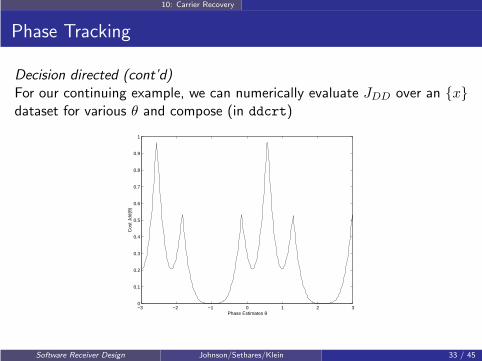
Decision directed (cont’d)For our continuing example, we can numerically evaluate JDD over an {x}dataset for various θ and compose (in ddcrt)
−3 −2 −1 0 1 2 30
0.1
0.2
0.3
0.4
0.5
0.6
0.7
0.8
0.9
1
Phase Estimates θ
Cos
t Jdd
(θ)
Software Receiver Design Johnson/Sethares/Klein 33 / 45
10: Carrier Recovery
Phase Tracking (cont’d)
Decision directed (cont’d)
◮ Maxima of the decision-directed cost function occur in “worst” casewhen x ≈ 0 but |Q{x}| = 1 so (Q{x} − x)2 ≈ 1.
◮ The decision-directed cost function has a minimum at the desiredlocation of θ = φ = −1 and at locations an integer multiple of π away.
◮ JDD also has other local minima making initialization critical toachieving the desired system behavior.
◮ Accordingly, a decision-directed cost (and associated adaptationalgorithm) is often used only to maintain lock and provide trackingwith low algorithmic complexity once initial carrier acquisition hasoccured.
Software Receiver Design Johnson/Sethares/Klein 34 / 45

10: Carrier Recovery
Phase Tracking
Decision directed (cont’d)Now we examine the approximation of the gradient of the decision-directedcost function by evaluating the gradient of JDD after swapping averageand differentiation (see Appendix G) under a small stepsize presumption
◮ Because ∂[Q{x}]/∂x = 0 almost everywhere
∂JDD
∂θ≈ avg
{
∂(Q{x(kT )} − x(kT ))2
∂θ
}
≈ −2avg
{
(Q{x(kT )} − x(kT ))∂x(kT )
∂θ
}
◮ For a basic mixer downconversion
x(iT ) = x(kTs)|k=Mi
= 2[LPF{r(kTs) cos(2πf0kTs + θ)}]|k=Mi
where r(kTs) = s(kTs) cos(2πf0kTs + φ)which we can use to form ∂x/∂θ.
Software Receiver Design Johnson/Sethares/Klein 35 / 45
10: Carrier Recovery
Phase Tracking
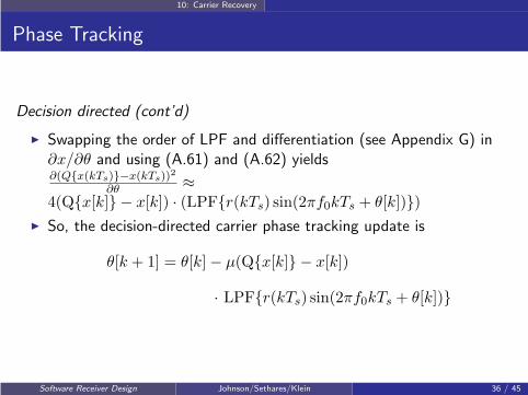
Decision directed (cont’d)
◮ Swapping the order of LPF and differentiation (see Appendix G) in∂x/∂θ and using (A.61) and (A.62) yields∂(Q{x(kTs)}−x(kTs))2
∂θ≈
4(Q{x[k]} − x[k]) · (LPF{r(kTs) sin(2πf0kTs + θ[k])})
◮ So, the decision-directed carrier phase tracking update is
θ[k + 1] = θ[k]− µ(Q{x[k]} − x[k])
· LPF{r(kTs) sin(2πf0kTs + θ[k])}
Software Receiver Design Johnson/Sethares/Klein 36 / 45
10: Carrier Recovery
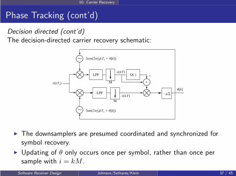
Phase Tracking (cont’d)
Decision directed (cont’d)The decision-directed carrier recovery schematic:
2mgLPFu[k]
LPFx(kT)
x(kT).
Q( )
2
1
2cos(2pf0kTs 1 u[k])
2sin(2pf0kTs 1 u[k])
r(kTs)
,
,
1M
M
◮ The downsamplers are presumed coordinated and synchronized forsymbol recovery.
◮ Updating of θ only occurs once per symbol, rather than once persample with i = kM .
Software Receiver Design Johnson/Sethares/Klein 37 / 45

10: Carrier Recovery
Phase Tracking (cont’d)
Decision directed (cont’d)Adapted θ trajectories (from plldd) for two starting points:
◮ θ[1] = −1.27 and µ = 0.03
0 0.2 0.4 0.6 0.8 1 1.2 1.4 1.6 1.8 2−1.28
−1.26
−1.24
−1.22
−1.2
−1.18
−1.16
−1.14
−1.12
−1.1
time
phas
e es
timat
es
◮ Slow convergence here is related to flatness of cost function in vicinityof global minimum.
Software Receiver Design Johnson/Sethares/Klein 38 / 45
10: Carrier Recovery
Phase Tracking (cont’d)
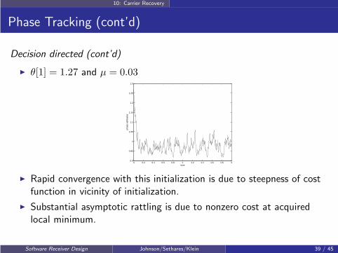
Decision directed (cont’d)
◮ θ[1] = 1.27 and µ = 0.03
0 0.2 0.4 0.6 0.8 1 1.2 1.4 1.6 1.8 20.9
0.95
1
1.05
1.1
1.15
1.2
1.25
1.3
time
phas
e es
timat
es
◮ Rapid convergence with this initialization is due to steepness of costfunction in vicinity of initialization.
◮ Substantial asymptotic rattling is due to nonzero cost at acquiredlocal minimum.
Software Receiver Design Johnson/Sethares/Klein 39 / 45

10: Carrier Recovery
Frequency Tracking
Consider the situation where both the receiver oscillator’s frequency andphase are off.
◮ Received signal
r(kTs) = s(kTs) cos(2πfckTs + φ)
◮ Receiver mixer LPF output assuming f0 − fc within LPF passband
y(kTs) = LPF{2r(kTs) cos(2πf0kTs + θ)}
= s(kTs) cos(2π(fc − f0)kTs + φ− θ)
◮ With θ adaptively adjusted as θ[k], perfect carrier recovery occursonly if
θ[k] = 2π(fc − f0)kTs + φ
Software Receiver Design Johnson/Sethares/Klein 40 / 45

10: Carrier Recovery
Frequency Tracking (cont’d)
◮ Single PLL produces
θ[k] → 2π(fc − f0)kTs + β
◮ With φ = −1, fc = 1000, f0 = 1001, and θ[1] = 0, PLL (frompllconverge) with a stepsize of 0.005 produces
0 0.2 0.4 0.6 0.8 1 1.2 1.4 1.6 1.8 2−14
−12
−10
−8
−6
−4
−2
0
2Phase Tracking via the Phase Locked Loop
time
phas
e of
fset
Software Receiver Design Johnson/Sethares/Klein 41 / 45

10: Carrier Recovery
Frequency Tracking (cont’d)
◮ From plot take θ(4000) = −3.4009 and θ(16000) = −10.9304 tocheck
2π(fc − f0)kTs + β = θ[k]
◮ For k = 4000, fc − f0 = −1, and Ts = .0001 we achieve fairagreement:
−2.5133 + β = −3.4009 ⇒ β ≈ −0.8876
−10.0531 + β = −10.9304 ⇒ β ≈ −0.8773
◮ With φ = −1, this means that single PLL is short by≈ −1− (−0.88) ≈ −0.12 between k = 4000 and k = 16, 000 andbeyond.
◮ Adding the phase estimate output of a first PLL to the feedback in asecond, allows the second loop to track the remaining constant phaseoffset in matching the carrier phase.
Software Receiver Design Johnson/Sethares/Klein 42 / 45
10: Carrier Recovery
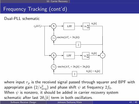
Frequency Tracking (cont’d)
Dual-PLL schematic
LPFrp(kTs)u1[k]
u2[k]
2m1a
2m2aLPF
sin(4pfckTs 1 2u1[k])
sin(4pfckTs 1 2u1[k] 1 2u2[k])
u1[k] 1 u2[k]
2
2
,
,
X
X 1
where input rp is the received signal passed through squarer and BPF withappropriate gain (2/s2avg) and phase shift ψ at frequency 2f0.When ψ is nonzero, it should be added in carrier recovery systemschematic after last 2θi[k] term in both oscillators.
Software Receiver Design Johnson/Sethares/Klein 43 / 45
10: Carrier Recovery
Frequency Tracking (cont’d)
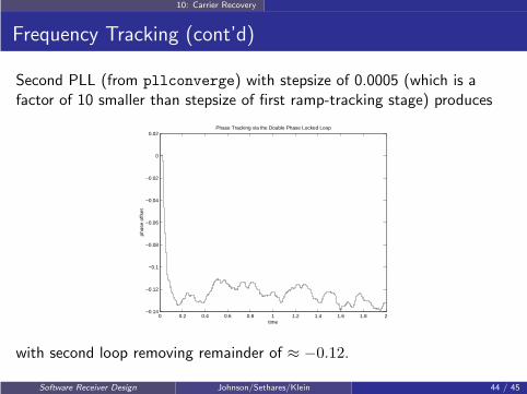
Second PLL (from pllconverge) with stepsize of 0.0005 (which is afactor of 10 smaller than stepsize of first ramp-tracking stage) produces
0 0.2 0.4 0.6 0.8 1 1.2 1.4 1.6 1.8 2−0.14
−0.12
−0.1
−0.08
−0.06
−0.04
−0.02
0
0.02Phase Tracking via the Double Phase Locked Loop
time
phas
e of
fset
with second loop removing remainder of ≈ −0.12.
Software Receiver Design Johnson/Sethares/Klein 44 / 45

10: Carrier Recovery
Frequency Tracking
◮ Could try squared difference approach to minimize average squareddifference between extracted carrier and reconstructed carrier withestimated frequency.
◮ Resulting squared difference cost function across frequency estimateas independent variable is flat with one deep well ⇒ not a goodsurface for a gradient descent search.
◮ Can add a second integrator to single PLL feedback loop asalternative to second PLL.
◮ Can use other phase trackers in dual configuration.
NEXT... We examine the pulse shape and receive filters that aid thetransition to (and from) an analog transmitted signal from (and to) adigital message sequence.
Software Receiver Design Johnson/Sethares/Klein 45 / 45