10 verification and validation of simulation models · prof. dr. mesut güneş ch. 10 verification...

10.1

Chapter 10

Verification and Validation of Simulation Models

Prof. Dr. Mesut Güneş ▪ Ch. 10 Verification and Validation of Simulation Models

10.2

Contents •  Model-Building, Verification, and Validation •  Verification of Simulation Models •  Calibration and Validation


10.3

Purpose & Overview •  The goal of the validation process is:

• To produce a model that represents true behavior closely enough for decision-making purposes

• To increase the model’s credibility to an acceptable level

•  Validation is an integral part of model development: • Verification: building the model

correctly, correctly implemented with good input and structure

• Validation: building the correct model, an accurate representation of the real system

•  Most methods are informal subjective comparisons while a few are formal statistical procedures


10.4

Modeling-Building, Verification & Validation


10.5

Modeling-Building, Verification & Validation •  Steps in Model-Building

• Real system •  Observe the real system •  Interactions among the

components •  Collecting data on the

behavior

• Conceptual model Construction of a conceptual model

• Simulation program Implementation of an operational model


10.6

Verification •  Purpose: ensure the conceptual model is reflected accurately in

the computerized representation. •  Many common-sense suggestions, for example:

• Have someone else check the model. • Make a flow diagram that includes each logically possible action a

system can take when an event occurs. • Closely examine the model output for reasonableness under a variety

of input parameter settings. • Print the input parameters at the end of the simulation, make sure

they have not been changed inadvertently. • Make the operational model as self-documenting as possible. • If the operational model is animated, verify that what is seen in the

animation imitates the actual system. • Use the debugger. • If possible use a graphical representation of the model.


10.7

Examination of Model Output for Reasonableness •  Two statistics that give a quick indication of model

reasonableness are current contents and total counts

• Current content: The number of items in each component of the system at a given time.

• Total counts: Total number of items that have entered each component of the system by a given time.

•  Compute certain long-run measures of performance, e.g. compute the long-run server utilization and compare to simulation results.


10.8

Examination of Model Output for Reasonableness

•  A model of a complex network of queues consisting of many service centers. • If the current content grows in a more or less linear fashion as the simulation run time increases, it is likely that a queue is unstable

• If the total count for some subsystem is zero, indicates no items entered that subsystem, a highly suspect occurrence

• If the total and current count are equal to one, can indicate that an entity has captured a resource but never freed that resource.


10.9

Documentation

•  Documentation • A means of clarifying the logic of a model and verifying its completeness.

• Comment the operational model •  definition of all variables (default values?) •  definition of all constants (default values?) •  functions and parameters •  relationship of objects •  etc.

•  Default values should be explained!


10.10

Trace •  A trace is a detailed printout of the state of the simulation

model over time. •  Can be very labor intensive if the programming language

does not support statistic collection. •  Labor can be reduced by a centralized tracing mechanism •  In object-oriented simulation framework, trace support

can be integrated into class hierarchy. New classes need only to add little for the trace support.


10.11

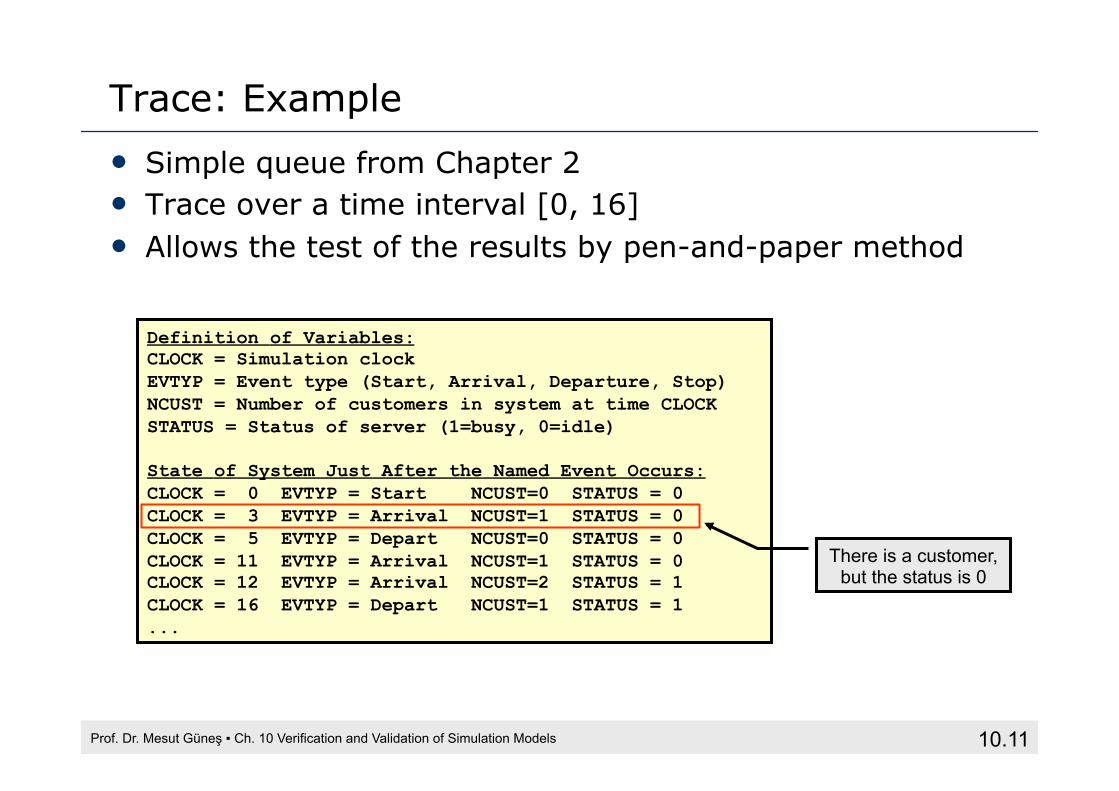
Trace: Example •  Simple queue from Chapter 2 •  Trace over a time interval [0, 16] •  Allows the test of the results by pen-and-paper method


Definition of Variables: CLOCK = Simulation clock EVTYP = Event type (Start, Arrival, Departure, Stop) NCUST = Number of customers in system at time CLOCK STATUS = Status of server (1=busy, 0=idle) State of System Just After the Named Event Occurs: CLOCK = 0 EVTYP = Start NCUST=0 STATUS = 0 CLOCK = 3 EVTYP = Arrival NCUST=1 STATUS = 0 CLOCK = 5 EVTYP = Depart NCUST=0 STATUS = 0 CLOCK = 11 EVTYP = Arrival NCUST=1 STATUS = 0 CLOCK = 12 EVTYP = Arrival NCUST=2 STATUS = 1 CLOCK = 16 EVTYP = Depart NCUST=1 STATUS = 1 ...

There is a customer, but the status is 0

10.12

Calibration and Validation


10.13

Calibration and Validation •  Validation: the overall process of comparing the model

and its behavior to the real system. •  Calibration: the iterative process of comparing the model

to the real system and making adjustments.

•  Comparison of the model to real system • Subjective tests

•  People who are knowledgeable about the system

• Objective tests •  Requires data on the real

system’s behavior and the output of the model


10.14

Calibration and Validation •  Danger during the calibration phase

• Typically few data sets are available, in the worst case only one, and the model is only validated for these.

• Solution: If possible collect new data sets

•  No model is ever a perfect representation of the system • The modeler must weigh the possible, but not guaranteed, increase in model accuracy versus the cost of increased validation effort.


10.15

Calibration and Validation •  Three-step approach for validation:

1.  Build a model that has high face validity

2.  Validate model assumptions

3.  Compare the model input-output transformations with the real system’s data


10.16

Validation: 1. High Face Validity •  Ensure a high degree of realism:

• Potential users should be involved in model construction from its conceptualization to its implementation.

•  Sensitivity analysis can also be used to check a model’s face validity. • Example: In most queueing systems, if the arrival rate of customers were to increase, it would be expected that server utilization, queue length and delays would tend to increase.

• For large-scale simulation models, there are many input variables and thus possibly many sensitivity tests. •  Sometimes not possible to perform all of theses tests, select the

most critical ones.


10.17

Validation: 2. Validate Model Assumptions •  General classes of model assumptions:

• Structural assumptions: how the system operates. • Data assumptions: reliability of data and its statistical analysis.

•  Bank example: customer queueing and service facility in a bank. • Structural assumptions

•  Customer waiting in one line versus many lines •  Customers are served according FCFS versus priority

• Data assumptions, e.g., interarrival time of customers, service times for commercial accounts. •  Verify data reliability with bank managers •  Test correlation and goodness of fit for data


10.18

Validation: 3. Validate Input-Output Transformation

•  Goal: Validate the model’s ability to predict future behavior • The only objective test of the model. • The structure of the model should be accurate enough to make good

predictions for the range of input data sets of interest. •  One possible approach: use historical data that have been

reserved for validation purposes only. •  Criteria: use the main responses of interest.


System Input Output

Model Output Input

Model is viewed as an input-output

transformation

10.19

Bank Example

Example: One drive-in window serviced by one teller, only one or two transactions are allowed.

•  Data collection: 90 customers during 11am to 1pm • Observed service times {Si, i =1,2, …, 90} • Observed interarrival times {Ai, i =1,2, …, 90}

•  Data analysis let to the conclusion that: • Interarrival times: exponentially distributed with rate λ = 45/hour

• Service times: N(1.1, 0.22)


Input variables

10.20

Bank Example: The Black Box

•  A model was developed in close consultation with bank management and employees

•  Model assumptions were validated •  Resulting model is now viewed as a “black box”:


Uncontrolled variables, X

Controlled Decision variables, D

Model “black box”

f(X,D) = Y

Input Variables Poisson arrivals λ = 45/hr: X11, X12, … Services times, N(D2, 0.22): X21, X22, … D1 = 1 (one teller) D2 = 1.1 min (mean service time) D3 = 1 (one line)

Model Output Variables, Y Primary interest: Y1 = teller’s utilization Y2 = average delay Y3 = maximum line length Secondary interest: Y4 = observed arrival rate Y5 = average service time Y6 = sample std. dev. of service times Y7 = average length of time

10.21

Bank Example: Comparison with Real System Data

•  Real system data are necessary for validation. • System responses should have been collected during the same time

period (from 11am to 1pm on the same day.)

•  Compare average delay from the model Y2 with actual delay Z2: • Average delay observed Z2 = 4.3 minutes • Consider this to be the true mean value µ0 = 4.3

• When the model is run with generated random variates X1n and X2n, Y2 should be close to Z2


10.22

Bank Example: Comparison with Real System Data •  Six statistically independent replications of the model,

each of 2-hour duration, are run.


Replication

Y4

Arrivals/Hour Y5

Service Time [Minutes] Y2

Average Delay [Minutes]

1 51.0 1.07 2.79 2 40.0 1.12 1.12 3 45.5 1.06 2.24 4 50.5 1.10 3.45 5 53.0 1.09 3.13 6 49.0 1.07 2.38

Sample mean [Delay] 2.51 Standard deviation [Delay] 0.82

10.23

Bank Example: Hypothesis Testing •  Compare the average delay from the model Y2 with the actual

delay Z2

• Null hypothesis testing: evaluate whether the simulation and the real system are the same (w.r.t. output measures):

•  If H0 is not rejected, then, there is no reason to consider the model invalid

•  If H0 is rejected, the current version of the model is rejected, and the modeler needs to improve the model


minutes 3.4minutes 34

21

20

≠

=

): E(YH.): E(YH

10.24

Bank Example: Hypothesis Testing •  Conduct the t test:

• Chose level of significance (α = 0.05) and sample size (n = 6). • Compute the sample mean and sample standard deviation over the n replications:

• Compute test statistics:

• Hence, reject H0. •  Conclude that the model is inadequate.

• Check: the assumptions justifying a t test, that the observations (Y2i) are normally and independently distributed.


minutes 51.211

22 == ∑=

n

iiYn

Yminutes 82.0

1

)(1

222

=−

−=∑=

n

YYS

n

ii

t0 =Y2 −µ0

S / n=

2.51− 4.3 0.82 / 6

= 5.34 > t0.025,5 = 2.571 (for a 2-sided test)

10.25

Bank Example: Hypothesis Testing

•  Similarly, compare the model output with the observed output for other measures:

Y4 ↔ Z4

Y5 ↔ Z5

Y6 ↔ Z6


10.26

Power of a test


10.27

Power of a test •  For validation:

• Consider failure to reject H0 as a strong conclusion, the modeler would want β to be small.


The power of a test is the probability of detecting an invalid model.

Power =1−P(failing to reject H0 |H1 is true)=1−P(Type II error)=1−β

10.28

Power of a test •  Value of β depends on:

• Sample size n • The true difference, δ, between E(Y) and µ

•  In general, the best approach to control β is: • Specify the critical difference, δ. • Choose a sample size, n, by making use of the operating

characteristics curve (OC curve).


σ

µδ

−=

)(YE

10.29

Power of a test •  Operating characteristics

curve (OC curve). • Graphs of the probability of a

Type II Error β(δ) versus δ for a given sample size n


For the same error probability with smaller difference the required sample size increases!

10.30

Power of a test

•  Type I error (α): • Error of rejecting a valid model. • Controlled by specifying a small level of significance α.

•  Type II error (β): • Error of accepting a model as valid when it is invalid. • Controlled by specifying critical difference and find the n.

•  For a fixed sample size n, increasing α will decrease β.


Statistical Terminology Modeling Terminology Associated Risk Type I: rejecting H0 when H0 is true Rejecting a valid model α Type II: failure to reject H0 when H1 is true Failure to reject an invalid

model β

10.31

Confidence interval testing


10.32

Confidence Interval Testing

•  Confidence interval testing: evaluate whether the simulation and the real system performance measures are close enough.

•  If Y is the simulation output and µ = E(Y) •  The confidence interval (CI) for µ is:


⎥⎦

⎤⎢⎣

⎡+− −− n

StYnStY nn 1,1, 22, αα

10.33

Confidence Interval Testing

•  CI does not contain µ0: •  If the best-case error is > ε, model

needs to be refined. •  If the worst-case error is ≤ ε,

accept the model. •  If best-case error is ≤ ε, additional

replications are necessary.

•  CI contains µ0: •  If either the best-case or worst-

case error is > ε, additional replications are necessary.

•  If the worst-case error is ≤ ε, accept the model.


ε is a difference value chosen by the analyst, that is small enough to allow valid decisions to be

based on simulations!

µ0 is the unknown true value

10.34

Confidence Interval Testing •  Bank example: µ0 = 4.3, and “close enough” is ε = 1 minute of

expected customer delay. • A 95% confidence interval, based on the 6 replications is

[1.65, 3.37] because:

•  µ0 = 4.3 falls outside the confidence interval, •  the best case |3.37 – 4.3| = 0.93 < 1, but •  the worst case |1.65 – 4.3| = 2.65 > 1

" Additional replications are needed to reach a decision.


682.0571.251.2

5,025.0

±

±nStY

10.35

Other approaches


10.36

Using Historical Output Data

•  An alternative to generating input data: • Use the actual historical record. • Drive the simulation model with the historical record and then

compare model output to system data. • In the bank example, use the recorded interarrival and service times

for the customers {An, Sn, n = 1,2,…}.

•  Procedure and validation process: similar to the approach used for system generated input data.


10.37

Using a Turing Test

•  Use in addition to statistical test, or when no statistical test is readily applicable.

•  Utilize persons’ knowledge about the system. •  For example:

• Present 10 system performance reports to a manager of the system. Five of them are from the real system and the rest are “fake” reports based on simulation output data.

• If the person identifies a substantial number of the fake reports, interview the person to get information for model improvement.

• If the person cannot distinguish between fake and real reports with consistency, conclude that the test gives no evidence of model inadequacy.


Turing Test Described by Alan Turing in 1950. A human jugde is involved in a natural language conversation with a human and a machine. If the judge cannot reliably tell which of the partners is the machine, then the machine has passed the test.

10.38

Summary •  Model validation is essential:

• Model verification • Calibration and validation • Conceptual validation

•  Best to compare system data to model data, and make comparison using a wide variety of techniques.

•  Some techniques that we covered: • Insure high face validity by consulting knowledgeable persons. • Conduct simple statistical tests on assumed distributional forms. • Conduct a Turing test. • Compare model output to system output by statistical tests.


10 verification and validation of simulation models · prof. dr. mesut güneş ch. 10 verification...

Documents