10.1 Comparing Two

Proportions

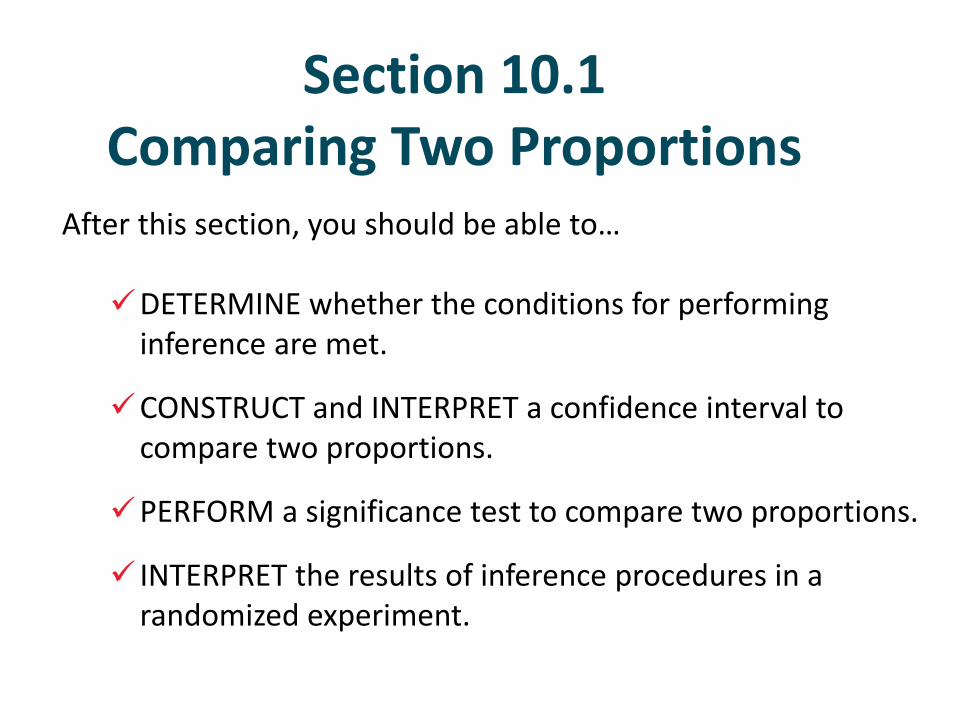
Section 10.1Comparing Two Proportions

After this section, you should be able to…

✓DETERMINE whether the conditions for performing inference are met.

✓CONSTRUCT and INTERPRET a confidence interval to compare two proportions.

✓PERFORM a significance test to compare two proportions.

✓ INTERPRET the results of inference procedures in a randomized experiment.

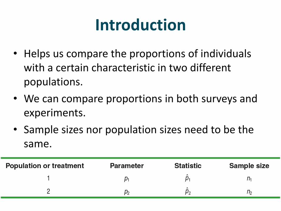
Introduction

• Helps us compare the proportions of individuals with a certain characteristic in two different populations.

• We can compare proportions in both surveys and experiments.

• Sample sizes nor population sizes need to be the same.

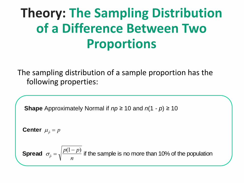
Theory: The Sampling Distribution of a Difference Between Two

Proportions

The sampling distribution of a sample proportion has the following properties:

Shape Approximately Normal if np ≥ 10 and n(1 - p) ≥ 10

Center ˆ p p

Spread ˆ p p(1 p)

n if the sample is no more than 10% of the population

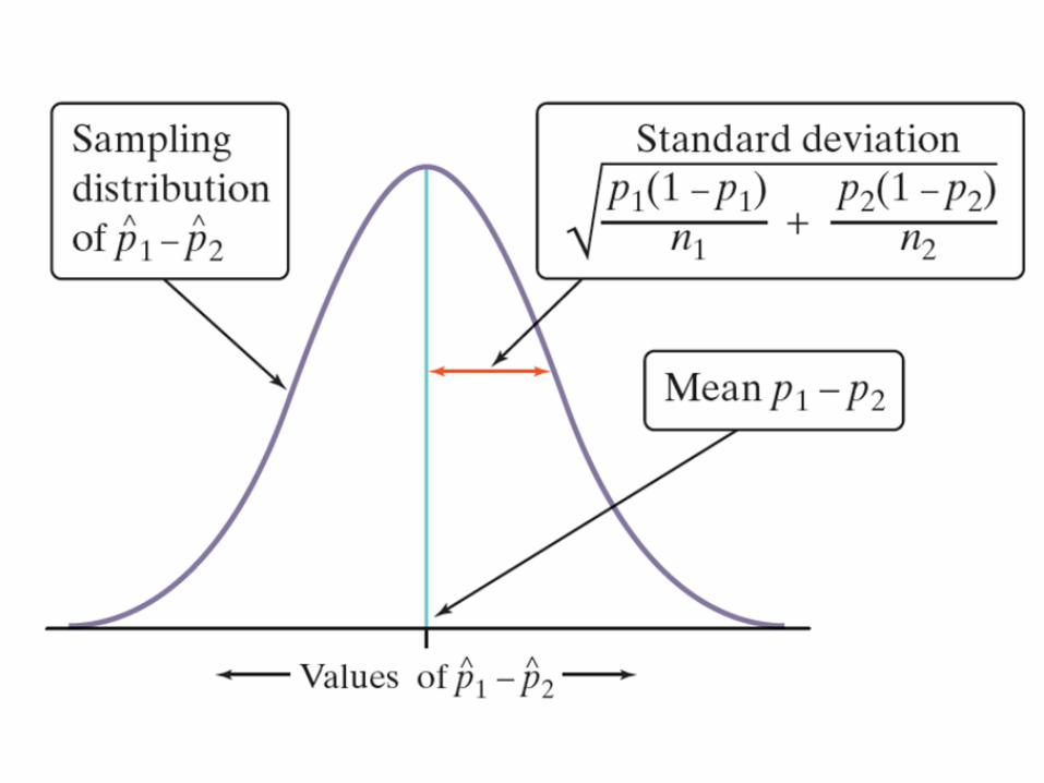
Theory: The Sampling Distribution of a Difference Between Two Proportions

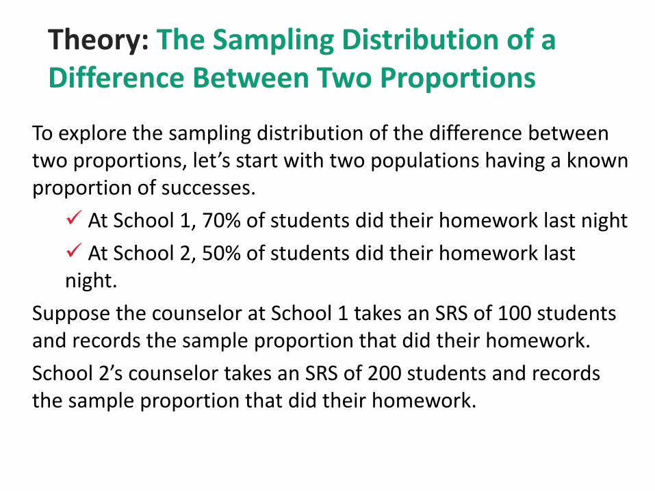
To explore the sampling distribution of the difference between two proportions, let’s start with two populations having a known proportion of successes.

✓ At School 1, 70% of students did their homework last night

✓ At School 2, 50% of students did their homework last night.

Suppose the counselor at School 1 takes an SRS of 100 students and records the sample proportion that did their homework.

School 2’s counselor takes an SRS of 200 students and records the sample proportion that did their homework.

Theory: The Sampling Distribution of a Difference Between Two Proportions

Using Fathom software, we generated an SRS of 100 students from School 1 and a separate SRS of 200 students from School 2. The difference in sample proportions was then calculated and plotted. We repeated this process 1000 times. The results are below:

What do you notice about the shape, center, and spreadof the sampling distribution of ˆ p 1 ˆ p 2 ?

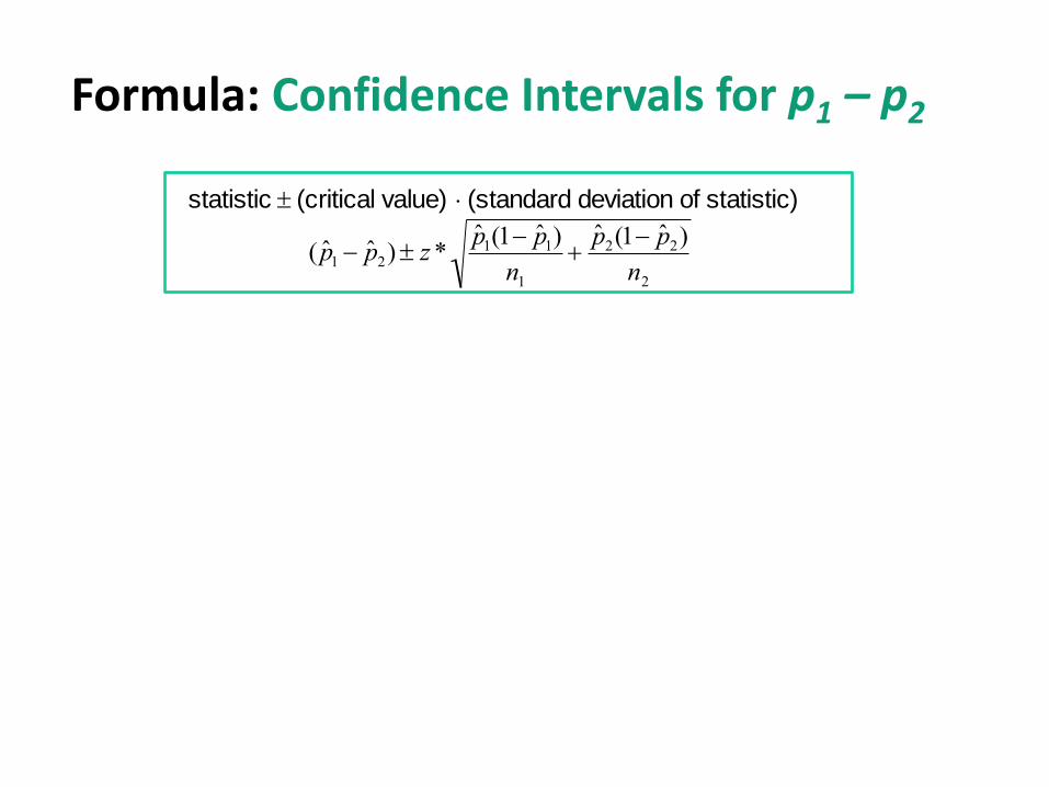
Formula: Confidence Intervals for p1 – p2

statistic (critical value) (standard deviation of statistic)

( ˆ p 1 ˆ p 2) z *ˆ p 1(1 ˆ p 1)

n1

ˆ p 2(1 ˆ p 2)

n2

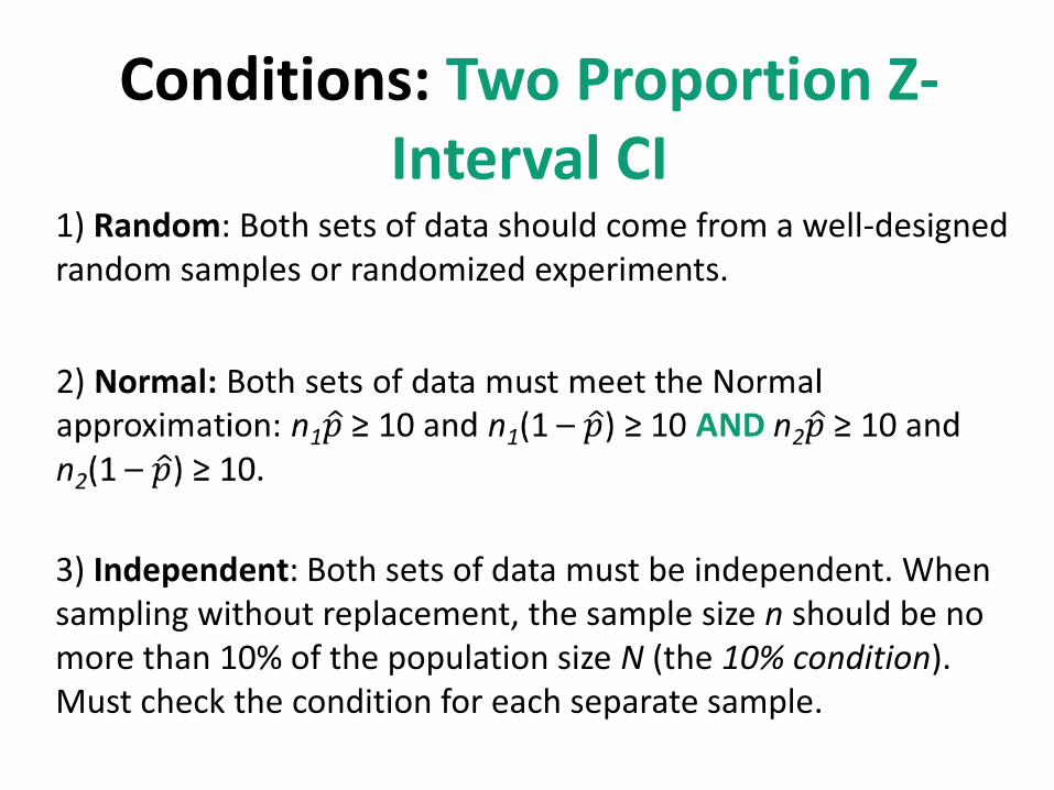
Conditions: Two Proportion Z-Interval CI

1) Random: Both sets of data should come from a well-designed random samples or randomized experiments.

3) Independent: Both sets of data must be independent. When sampling without replacement, the sample size n should be no more than 10% of the population size N (the 10% condition). Must check the condition for each separate sample.

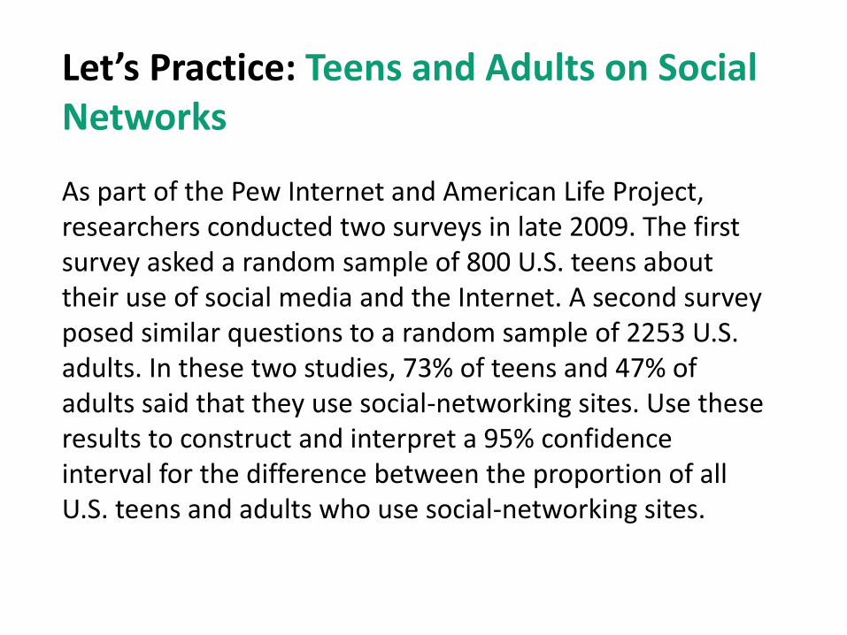
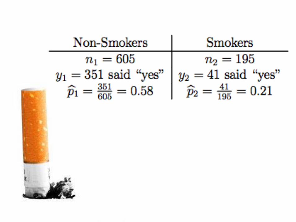
Let’s Practice: Teens and Adults on Social Networks

As part of the Pew Internet and American Life Project, researchers conducted two surveys in late 2009. The first survey asked a random sample of 800 U.S. teens about their use of social media and the Internet. A second survey posed similar questions to a random sample of 2253 U.S. adults. In these two studies, 73% of teens and 47% of adults said that they use social-networking sites. Use these results to construct and interpret a 95% confidence interval for the difference between the proportion of all U.S. teens and adults who use social-networking sites.

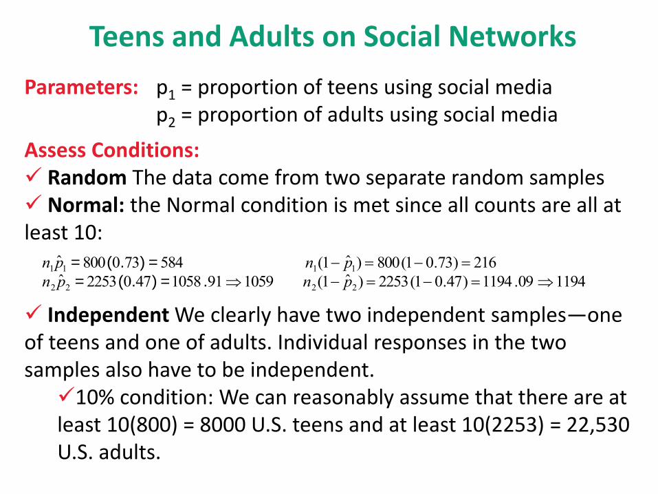
Assess Conditions:✓ Random The data come from two separate random samples✓ Normal: the Normal condition is met since all counts are all at least 10:

✓ Independent We clearly have two independent samples—one of teens and one of adults. Individual responses in the two samples also have to be independent.

✓10% condition: We can reasonably assume that there are at least 10(800) = 8000 U.S. teens and at least 10(2253) = 22,530 U.S. adults.

Teens and Adults on Social Networks

n1ˆ p 1 = 800(0.73) = 584 n1(1 ˆ p 1) 800(1 0.73) 216

n2ˆ p 2 = 2253(0.47) =1058 .911059 n2(1 ˆ p 2) 2253(1 0.47) 1194 .09 1194

Parameters: p1 = proportion of teens using social mediap2 = proportion of adults using social media

Teens and Adults on Social Networks

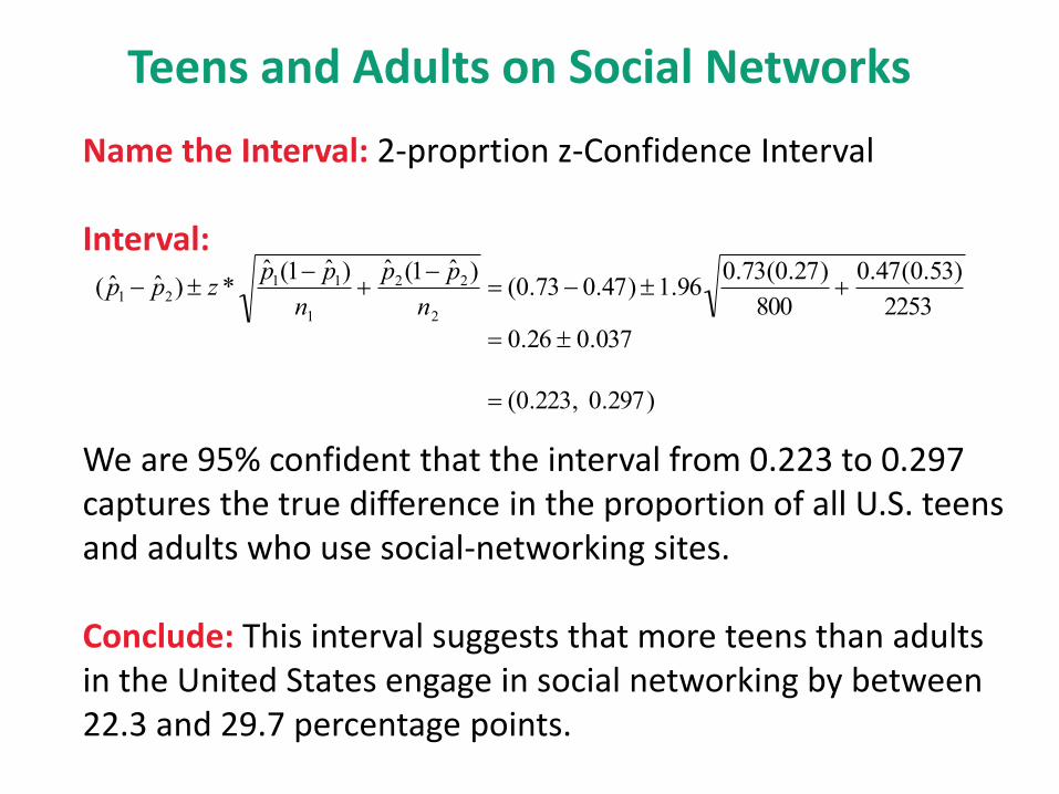
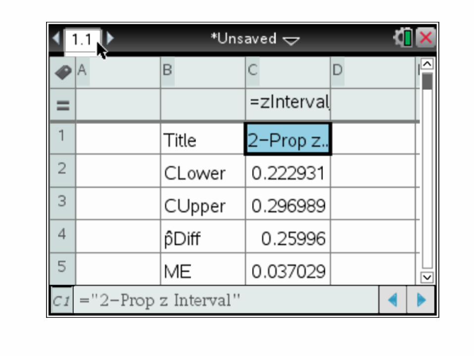
Name the Interval: 2-proprtion z-Confidence Interval

Interval:

We are 95% confident that the interval from 0.223 to 0.297 captures the true difference in the proportion of all U.S. teens and adults who use social-networking sites.

Conclude: This interval suggests that more teens than adults in the United States engage in social networking by between 22.3 and 29.7 percentage points.

( ˆ p 1 ˆ p 2) z *ˆ p 1(1 ˆ p 1)

n1

ˆ p 2(1 ˆ p 2)

n2

(0.73 0.47) 1.960.73(0.27)

800

0.47(0.53)

2253

0.26 0.037

(0.223, 0.297)

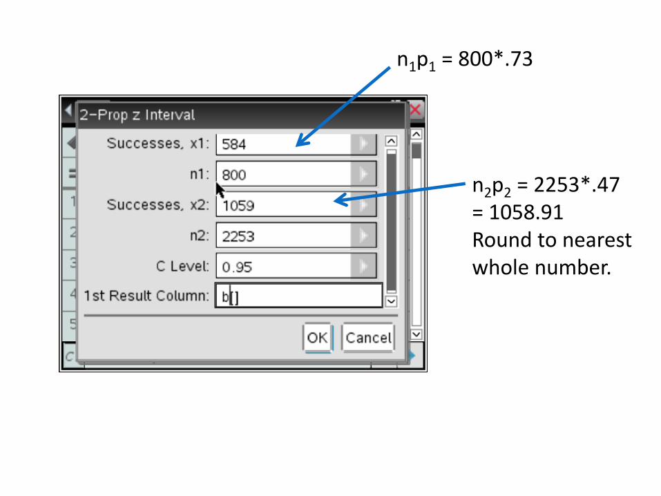
n1p1 = 800*.73

n2p2 = 2253*.47= 1058.91Round to nearest whole number.

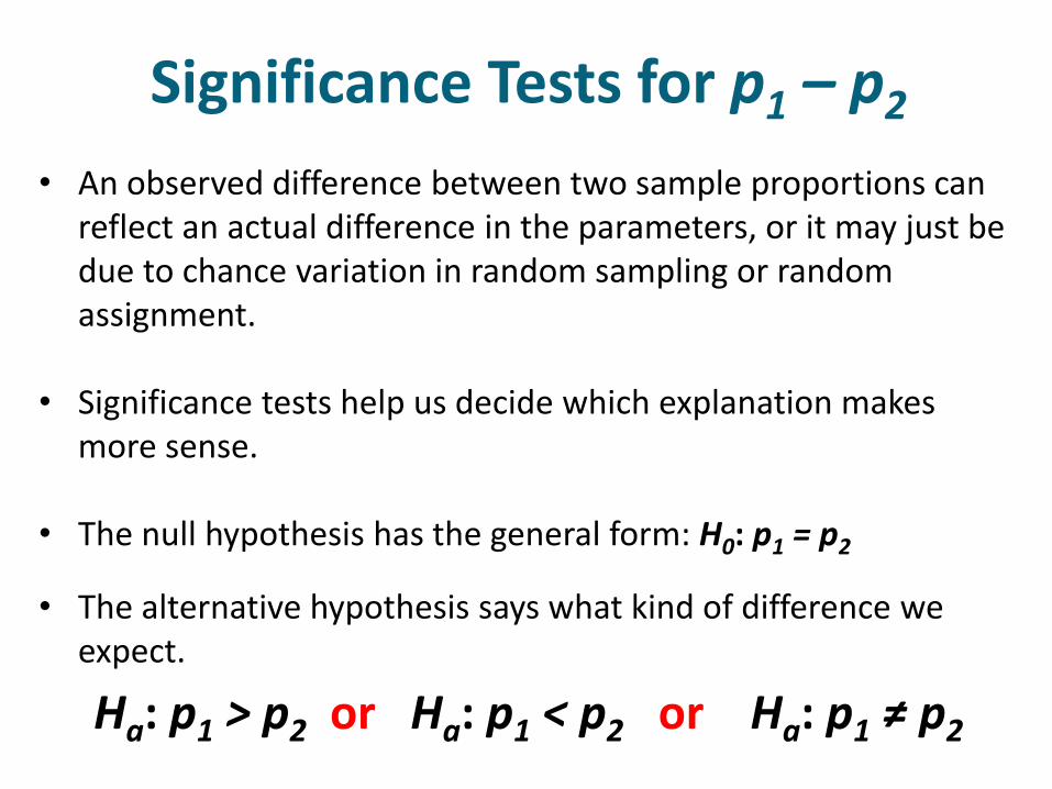
• An observed difference between two sample proportions can reflect an actual difference in the parameters, or it may just be due to chance variation in random sampling or random assignment.

• Significance tests help us decide which explanation makes more sense.

• The null hypothesis has the general form: H0: p1 = p2

• The alternative hypothesis says what kind of difference we expect.

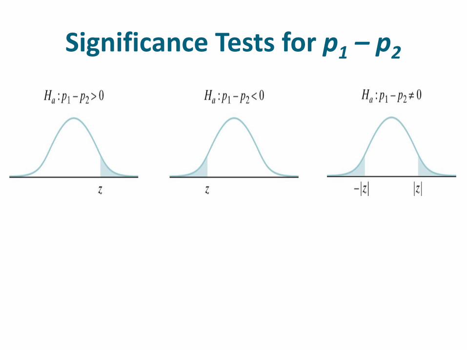
Ha: p1 > p2 or Ha: p1 < p2 or Ha: p1 ≠ p2

Significance Tests for p1 – p2

Significance Tests for p1 – p2

Significance Tests for p1 – p2

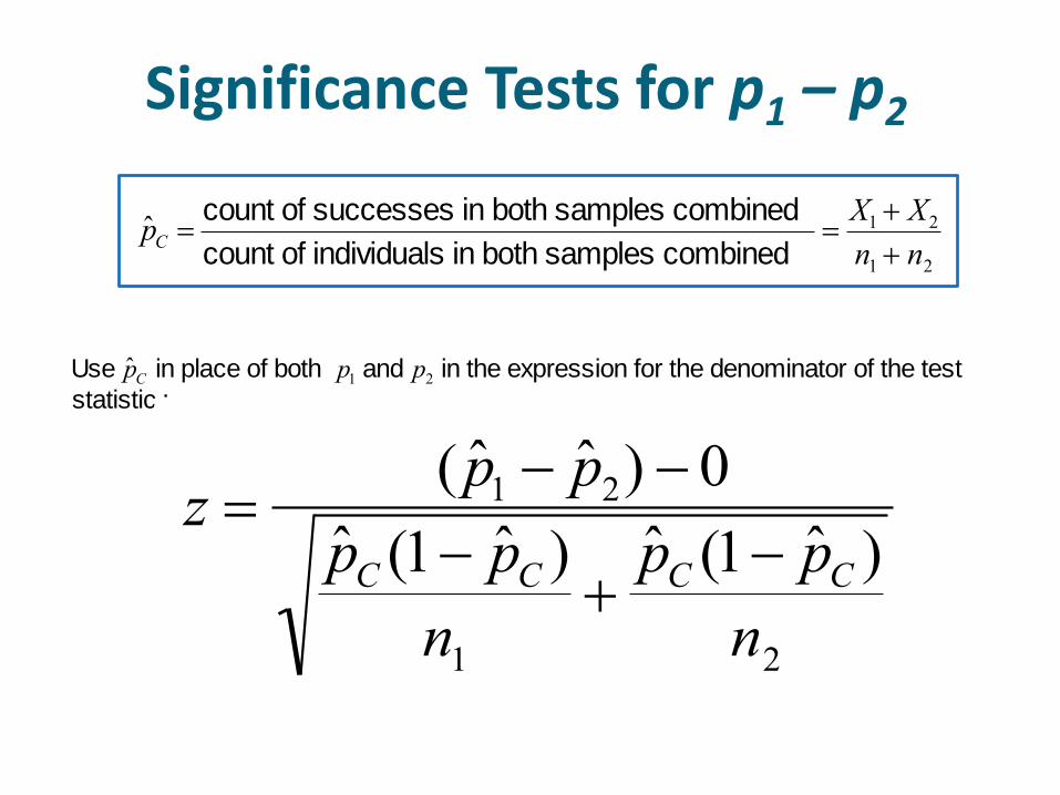
ˆ p C count of successes in both samples combined

count of individuals in both samples combined

X1 X2

n1 n2

Use ˆ p C in place of both p1 and p2 in the expression for the denominator of the test

statistic :

z ( ˆ p 1 ˆ p 2) 0

ˆ p C (1 ˆ p C )

n1

ˆ p C (1 ˆ p C )

n2

Use ˆ p C in place of both p1 and p2 in the expression for the denominator of the test

statistic :

z ( ˆ p 1 ˆ p 2) 0

ˆ p C (1 ˆ p C )

n1

ˆ p C (1 ˆ p C )

n2

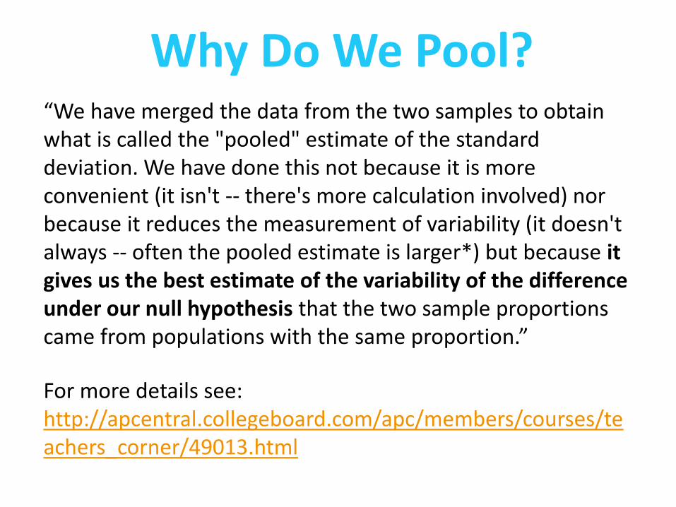
Why Do We Pool?“We have merged the data from the two samples to obtain what is called the "pooled" estimate of the standard deviation. We have done this not because it is more convenient (it isn't -- there's more calculation involved) nor because it reduces the measurement of variability (it doesn't always -- often the pooled estimate is larger*) but because it gives us the best estimate of the variability of the difference under our null hypothesis that the two sample proportions came from populations with the same proportion.”

For more details see: http://apcentral.collegeboard.com/apc/members/courses/teachers_corner/49013.html

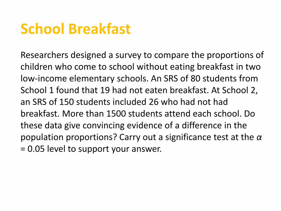
School Breakfast

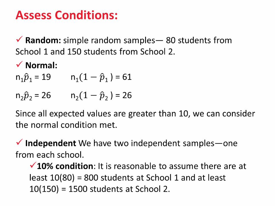
Researchers designed a survey to compare the proportions of children who come to school without eating breakfast in two low-income elementary schools. An SRS of 80 students from School 1 found that 19 had not eaten breakfast. At School 2, an SRS of 150 students included 26 who had not had breakfast. More than 1500 students attend each school. Do these data give convincing evidence of a difference in the population proportions? Carry out a significance test at the α= 0.05 level to support your answer.

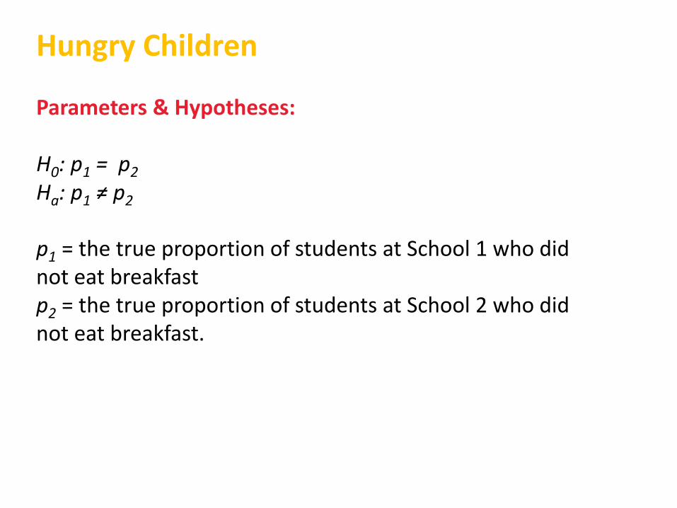
Hungry Children

Parameters & Hypotheses:

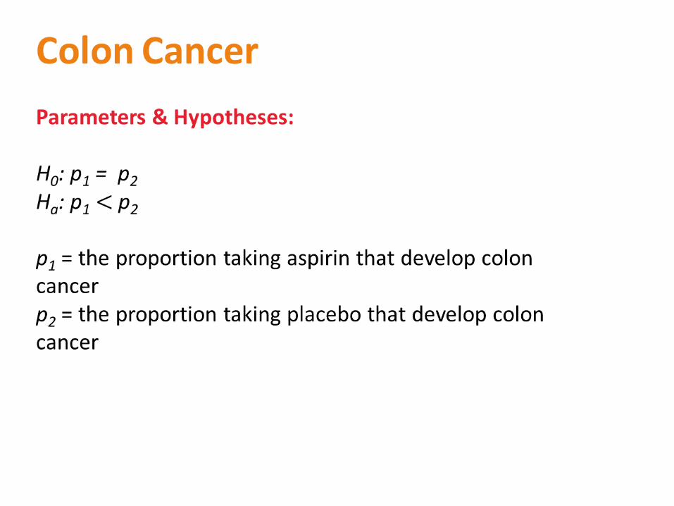
H0: p1 = p2

Ha: p1 ≠ p2

p1 = the true proportion of students at School 1 who did not eat breakfastp2 = the true proportion of students at School 2 who did not eat breakfast.

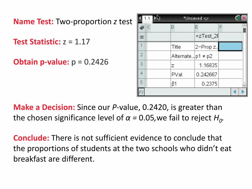
Name Test: Two-proportion z test

Test Statistic: z = 1.17

Obtain p-value: p = 0.2426

Make a Decision: Since our P-value, 0.2420, is greater than the chosen significance level of α = 0.05,we fail to reject H0.

Conclude: There is not sufficient evidence to conclude that the proportions of students at the two schools who didn’t eat breakfast are different.

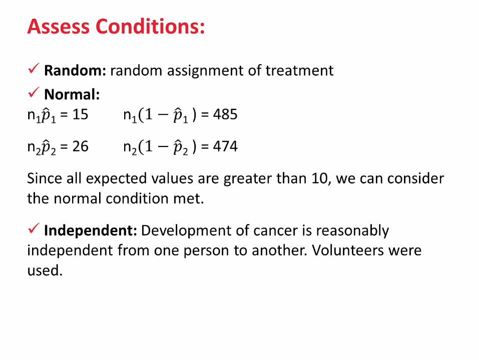
Colon Cancer: FRQ 2015 # 4

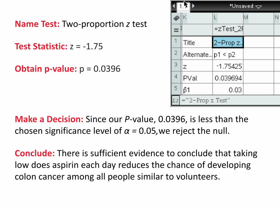
Name Test: Two-proportion z test

Test Statistic: z = -1.75

Obtain p-value: p = 0.0396

Make a Decision: Since our P-value, 0.0396, is less than the chosen significance level of α = 0.05,we reject the null.

Conclude: There is sufficient evidence to conclude that taking low does aspirin each day reduces the chance of developing colon cancer among all people similar to volunteers.

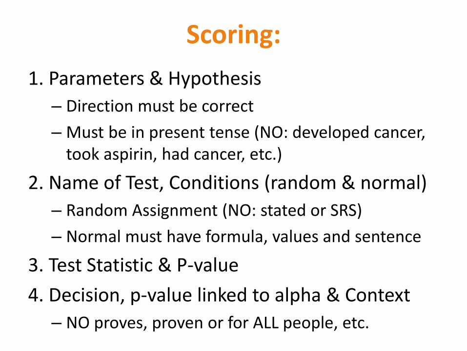
Scoring:

1. Parameters & Hypothesis

– Direction must be correct

– Must be in present tense (NO: developed cancer, took aspirin, had cancer, etc.)

2. Name of Test, Conditions (random & normal)

– Random Assignment (NO: stated or SRS)

– Normal must have formula, values and sentence

3. Test Statistic & P-value

4. Decision, p-value linked to alpha & Context

– NO proves, proven or for ALL people, etc.

Standard Error

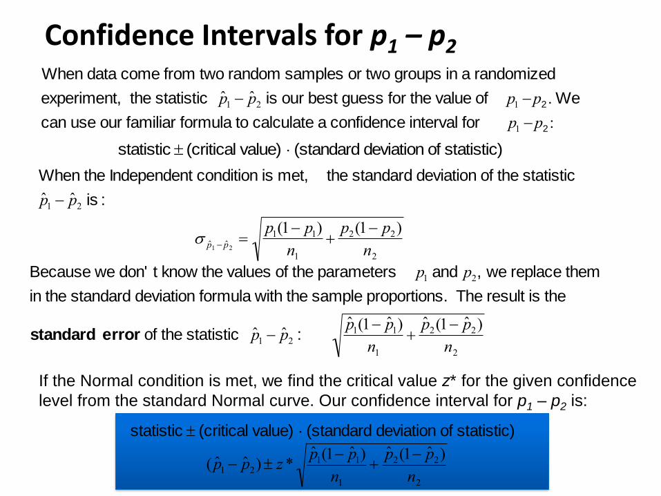
Confidence Intervals for p1 – p2

When data come from two random samples or two groups in a randomized

experiment, the statistic ˆ p 1 ˆ p 2 is our best guess for the value of p1 p2 . We

can use our familiar formula to calculate a confidence interval for p1 p2:

statistic (critical value) (standard deviation of statistic)

When the Independent condition is met, the standard deviation of the statistic

ˆ p 1 ˆ p 2 is :

ˆ p 1 ˆ p 2

p1(1 p1)

n1

p2(1 p2)

n2

Because we don' t know the values of the parameters p1 and p2, we replace them

in the standard deviation formula with the sample proportions. The result is the

standard error of the statistic ˆ p 1 ˆ p 2 : ˆ p 1(1 ˆ p 1)

n1

ˆ p 2(1 ˆ p 2)

n2

If the Normal condition is met, we find the critical value z* for the given confidence

level from the standard Normal curve. Our confidence interval for p1 – p2 is:

statistic (critical value) (standard deviation of statistic)

( ˆ p 1 ˆ p 2) z *ˆ p 1(1 ˆ p 1)

n1

ˆ p 2(1 ˆ p 2)

n2