1051-455-20052 laboratories for physical optics
TRANSCRIPT
1051-455-20052Laboratories for Physical Optics
23 November 2005

Contents
Preface ix
1 Introduction 11.1 Introduction . . . . . . . . . . . . . . . . . . . . . . . . . . . . . . . . 11.2 Laboratory Notebook . . . . . . . . . . . . . . . . . . . . . . . . . . . 11.3 Laboratory Reports . . . . . . . . . . . . . . . . . . . . . . . . . . . . 2
1.3.1 Length of Laboratory Reports . . . . . . . . . . . . . . . . . . 41.3.2 Grammar and Syntax . . . . . . . . . . . . . . . . . . . . . . . 41.3.3 Equations . . . . . . . . . . . . . . . . . . . . . . . . . . . . . 4
1.4 Measurements and Error in Experiments . . . . . . . . . . . . . . . . 41.4.1 The Certainty of Uncertainty . . . . . . . . . . . . . . . . . . 41.4.2 Accuracy vs. Precision . . . . . . . . . . . . . . . . . . . . . . 51.4.3 Signi�cant Figures and Round-O¤ Error . . . . . . . . . . . . 51.4.4 Reading Vernier Scales . . . . . . . . . . . . . . . . . . . . . . 6
1.5 Propagation of Uncertainty (Error) . . . . . . . . . . . . . . . . . . . 71.5.1 Error of a Summation or Di¤erence . . . . . . . . . . . . . . . 81.5.2 Error of a Product or Ratio . . . . . . . . . . . . . . . . . . . 101.5.3 Value of a Measurement Raised to a Power . . . . . . . . . . . 111.5.4 Problems: . . . . . . . . . . . . . . . . . . . . . . . . . . . . . 12
2 Lab #1: Summation of Waves 132.1 Rationale: . . . . . . . . . . . . . . . . . . . . . . . . . . . . . . . . . 132.2 Preparation: . . . . . . . . . . . . . . . . . . . . . . . . . . . . . . . . 132.3 Equipment: . . . . . . . . . . . . . . . . . . . . . . . . . . . . . . . . 132.4 Procedure: . . . . . . . . . . . . . . . . . . . . . . . . . . . . . . . . . 14
2.4.1 Summation of 1-D oscillations using Wave.exe . . . . . . . . . 142.4.2 Summation of 1-D oscillations using Signals.exe . . . . . . . . 162.4.3 Summation of 1-D oscillations using Audacity.exe . . . . . . . 172.4.4 Orthogonal Summation of Oscillations using Wave.exe . . . . 182.4.5 Orthogonal Summation of Functions using Signals.exe . . . . 192.4.6 Nonlinear Operations on Sinusoidal Waves in Signals . . . . . 20
2.5 Questions: . . . . . . . . . . . . . . . . . . . . . . . . . . . . . . . . . 22
v
vi CONTENTS
3 Lab #2: Dispersion 233.1 References: . . . . . . . . . . . . . . . . . . . . . . . . . . . . . . . . 233.2 Rationale: . . . . . . . . . . . . . . . . . . . . . . . . . . . . . . . . . 233.3 Theory: . . . . . . . . . . . . . . . . . . . . . . . . . . . . . . . . . . 233.4 Equipment: . . . . . . . . . . . . . . . . . . . . . . . . . . . . . . . . 273.5 Procedure: . . . . . . . . . . . . . . . . . . . . . . . . . . . . . . . . . 283.6 Analysis: . . . . . . . . . . . . . . . . . . . . . . . . . . . . . . . . . . 303.7 Questions: . . . . . . . . . . . . . . . . . . . . . . . . . . . . . . . . . 30
4 Lab #3: Polarization 334.1 Background: . . . . . . . . . . . . . . . . . . . . . . . . . . . . . . . . 33
4.1.1 Cross Product . . . . . . . . . . . . . . . . . . . . . . . . . . . 334.1.2 Polarization . . . . . . . . . . . . . . . . . . . . . . . . . . . . 344.1.3 Nomenclature for Circular Polarization . . . . . . . . . . . . . 37
4.2 Equipment: . . . . . . . . . . . . . . . . . . . . . . . . . . . . . . . . 374.3 Procedure: . . . . . . . . . . . . . . . . . . . . . . . . . . . . . . . . . 384.4 Analysis: . . . . . . . . . . . . . . . . . . . . . . . . . . . . . . . . . . 414.5 Questions: . . . . . . . . . . . . . . . . . . . . . . . . . . . . . . . . . 42
5 Lab #4: Division-of-Wavefront Interference 435.1 Theory . . . . . . . . . . . . . . . . . . . . . . . . . . . . . . . . . . . 43
5.1.1 Interference: . . . . . . . . . . . . . . . . . . . . . . . . . . . . 435.2 Equipment: . . . . . . . . . . . . . . . . . . . . . . . . . . . . . . . . 465.3 Procedure: . . . . . . . . . . . . . . . . . . . . . . . . . . . . . . . . . 46
6 Lab #5: Division-of-Amplitude Interference 496.1 Theory: . . . . . . . . . . . . . . . . . . . . . . . . . . . . . . . . . . 49
6.1.1 Division-of-Wavefront Interferometry . . . . . . . . . . . . . . 496.1.2 Division-of-Amplitude Interferometry . . . . . . . . . . . . . . 506.1.3 Michelson Interferometer . . . . . . . . . . . . . . . . . . . . . 51
6.2 Equipment: . . . . . . . . . . . . . . . . . . . . . . . . . . . . . . . . 556.3 Procedure: . . . . . . . . . . . . . . . . . . . . . . . . . . . . . . . . . 556.4 Questions: . . . . . . . . . . . . . . . . . . . . . . . . . . . . . . . . . 566.5 References: . . . . . . . . . . . . . . . . . . . . . . . . . . . . . . . . 57
7 Lab #6: Di¤raction 597.1 Theory: . . . . . . . . . . . . . . . . . . . . . . . . . . . . . . . . . . 59
7.1.1 Fresnel Di¤raction . . . . . . . . . . . . . . . . . . . . . . . . 607.1.2 Fraunhofer Di¤raction . . . . . . . . . . . . . . . . . . . . . . 617.1.3 Fraunhofer Di¤raction in Optical Imaging Systems . . . . . . 63
7.2 Equipment: . . . . . . . . . . . . . . . . . . . . . . . . . . . . . . . . 667.3 Procedure: . . . . . . . . . . . . . . . . . . . . . . . . . . . . . . . . . 667.4 Questions . . . . . . . . . . . . . . . . . . . . . . . . . . . . . . . . . 69
CONTENTS vii
8 Lab #7: Fourier Optics 718.1 Theory: . . . . . . . . . . . . . . . . . . . . . . . . . . . . . . . . . . 718.2 Equipment: . . . . . . . . . . . . . . . . . . . . . . . . . . . . . . . . 728.3 Procedure: . . . . . . . . . . . . . . . . . . . . . . . . . . . . . . . . . 738.4 References: . . . . . . . . . . . . . . . . . . . . . . . . . . . . . . . . 75
9 Lab #8: Computer-Generated Holography 779.1 Theory: . . . . . . . . . . . . . . . . . . . . . . . . . . . . . . . . . . 779.2 Fraunhofer Hologram of Two Point Sources: . . . . . . . . . . . . . . 789.3 Equipment: . . . . . . . . . . . . . . . . . . . . . . . . . . . . . . . . 819.4 Procedure: . . . . . . . . . . . . . . . . . . . . . . . . . . . . . . . . . 81
9.4.1 Recipe for a Detour-Phase Hologram: . . . . . . . . . . . . . . 829.5 References: . . . . . . . . . . . . . . . . . . . . . . . . . . . . . . . . 85

Chapter 1
Introduction
1.1 Introduction
As a scientist, probably the most fundamental means you will use to communicatewith colleagues is through reports and papers that summarize your research. Thematerial you will write about is often complex and non-intuitive. Because of thisfact, it is very important that you learn to write these reports clearly and concisely.To do this well often requires signi�cant practice. Laboratory reports are one of themore important opportunities to develop in this area.In real research, the utility of an experiment is to test some hypothesis or theoret-
ical model. In the labs you will implement this quarter, the theory is well established.However, it will be very useful for you to approach these experiments from the pointof view that the theory is not well known; after all, this may well be your �rst intro-duction to the theory.The result of your experiments will fall into one of three categories:
1. the data support the theory within the experimental uncertainties,
2. the data do not support the theory within the experimental uncertainties, or
3. the experimental uncertainties do not allow for a meaningful comparison be-tween the data and the theory.
Conclusion (3) is often, if not usually, a disappointment, because it means thatone has to either admit severe de�ciencies in the data-taking technique or to revisitthe experimental method used and search for a better way to go about making themeasurement (of course, this is a very common outcome in real experiments!) How-ever, an honest researcher will report this when necessary. Each week, try to answerthe question: into which of these three categories does your experiment fall?
1.2 Laboratory Notebook
Students will perform the experiments in teams (ideally of two). Each laboratoryteam will keep a laboratory notebook that contains descriptions and diagrams of the
1
2 CHAPTER 1 INTRODUCTION
equipment used in each experiment setup, lists of all data collected, all computationsmade from those data, etc.Traditionally, laboratory notebooks are kept in a bound paper book with num-
bered pages that is made expressly for the purpose, but these days it is completelyappropriate in a classroom (rather than industrial) setting to keep an electronic note-book as a Wiki document or as a word processor document (e.g., Microsoft WordTM).In either case, the electronic notebook should include all data pasted from a spread-sheet (Microsoft ExcelTM) and diagrams from a sketching/drawing program. For thelatter, I use Microsoft PowerpointTM to make the drawings and then copy the imagesto Adobe PhotoshopTM (via �CTRL-C� to copy the drawing, then make a JPEGimage �le via �CTRL-N�and paste via �CTRL-V�in PhotoshopTM). All necessarysoftware for adding images and diagrams to the Wiki lab notebook is available on thecomputers in the labs. You should keep the lab notebook up to date as you are doingthe experiment; do NOT wait until after the lab period to �ll in the data.You are probably used to the expectation that you write a laboratory report for
each experiment. We are going to take a di¤erent tack in this course, where you keepa more complete laboratory notebook and write up only two experiments: one ofyour choice and one of the instructor�s choice. The format of the laboratory reportsis provided next.
1.3 Laboratory Reports
Though each team will keep one laboratory notebook, each student will electronicallysubmit TWO individual laboratory reports. The laboratories to be reported willinclude one each selected by the student and by the instructor.In your reports, remember the three C�s: concise, clear, and complete.The format for a laboratory report includes:Experiment TitleYour Name(Lab Partners�Names)Date of Experiment:Introduction or Abstract:Brief overview of the experiment providing any relevant background information,
the reason for the experiment, what you did, and any conclusions you reached.Experimental Method:Include a description of the equipment used with diagrams (not drawn by hand and
not copied from the lab descriptions, these drawings are to be made by the student).Include a discussion of how the experiment was performed in a concise summary inyour own words, rather than merely repeating the list of instructions provided in thewriteup.Data, Analysis, and Discussion:In each lab procedure handout, there will be a few questions that you will need to
answer. It usually is convenient to answer these questions in the conclusion. All datatables, graphs and calculations are to be integrated into the text rather than included
1.3 LABORATORY REPORTS 3
as appendices at the end of the document. You should include tables of all of rawdata with units and estimated measurement errors recorded during the experimentas well as all calculations.The details of your analysis and calculations must be explained. All equations for
the calculations are included along with a sample calculation.All graphs must include the following items:
1. Title;
2. Labeled axes with units;
3. Data points plotted must be shown with symbols and no connecting lines (thesize of the data point symbol should be chosen wisely);
4. Fits to data and/or theoretical curves should use lines with no symbols;
5. Computed coe¢ cients of any �ts of curves to data must be displayed on theplot;
6. Legends should be used if plotting more than one data set on a single graph.
You may use the graphing capabilities in Microsoft ExcelTM, but recognize thatits default format is not appropriate for most graphs. Please, please, PLEASE use awhite background in your graphs by turning o¤ the default �gray�background.Discuss your results and how they relate to theory. You need to compute the per-
cent di¤erence between the measured and theoretical values. Consider experimentalerrors and try and determine their most likely source. Try to determine the mostsigni�cant sources of possible experimental error rather than just listing all possibleerror sources.Diagrams of setups are particularly useful in lab reports. These can be very simple
�they do not have to be artistic. Include relevant dimensions that are necessary inany equations in the description.All required material in your lab writeup should be typed on a word processor,
both for ease of submission and for archiving. This includes equations, �gures, datatables, and answers to any questions. Handwritten pages will not be accepted. Includecaptions with �gures and data tables. Number your equations, data tables, and �guresand refer to them by number, e.g., �As demonstrated by Eq. 1, . . . �, �As shown inFig. 2, . . . �, etc. Equations are typically numbered in parentheses located �ush withthe right margin, while �gures and tables are numbered in their captions. The listsof equations, �gures, and tables are numbered separately.The general idea of the lab reports this quarter is to follow the format of real
research papers as closely as possible. If you would like some examples of what suchpapers really look like, go to the library or the CIS Reading Room and look througha couple of imaging science journals, e.g. Optical Engineering, the Journal ofthe Optical Society of America (JOSA), or the Journal of Imaging Scienceand Technology.Summary:
4 CHAPTER 1 INTRODUCTION
Finally summarize your �ndings and comment on your success (or lack of) inperforming the experiment.
1.3.1 Length of Laboratory Reports
There is no standard length to a lab report. To use a cliché, the lab report shouldbe as long as it must be, but no longer. You need to explain the concepts and theprocess su¢ ciently, but do not write pages of description when a few words and a�gure will su¢ ce.
1.3.2 Grammar and Syntax
Use whole sentences with appropriate grammar and syntax. Please do not use col-loquial or slang terms. Also, please PROOFREAD your reports before submission �and I don�t mean just check the spelling. You are practicing for your profession, sotake some pride in the results of your e¤orts and submit the best report that you can.
1.3.3 Equations
You will need to include equations and subscripts in your lab writeups, so you needto have the means to do so. Subscript fonts are available in most word processorsand equation fonts in many. For example, Microsoft WordTM includes a rudimentary�Equation Editor�, and add-on software (such as MathTypeTM from MathSoft) alsois available. You might consider investing in a scienti�c word processor that includesequation, graphing, and curve-�tting features � many are available, and the timeyou are likely to save over the course of your college career will easily outweigh thecost and learning time.As already mentioned, number any equations used in your lab writeup. Note that
the symbol �*�that is commonly used for multiplication in some disciplines is moreoften used to refer to the mathematical operation of convolution in imaging. I suggestthat you use either ���or ���to denote multiplication in lab reports, and NOT theletter �x.�The necessary symbols are available in most symbol fonts and you shouldbe using them in all of your documents and slide presentations.
1.4 Measurements and Error in Experiments
1.4.1 The Certainty of Uncertainty
Every measurement exhibits some associated uncertainty. A good experimentalist willtry to evaluate the level of uncertainty, which is speci�ed along with the measuredvalue (e.g., 10:4 � 0:1mm), which are then graphed as �error bars�along with themeasured numerical value). A very useful reference book on this subject is DataReduction and Error Analysis for the Physical Sciences (Third Edition), by PhilipBevington and D. Keith Robinson (McGraw-Hill, 2002, ISBN 0072472278). It is notunreasonable to say that this classic book should be on the shelf of every scientist.
1.4 MEASUREMENTS AND ERROR IN EXPERIMENTS 5
In these labs, it is very important for you to estimate the uncertainty. In partic-ular, it is helpful to decide which of the three possible categories mentioned in theintroduction that applies to your data. How can you do this? One way is to makewhat you think is a reasonable decision about the uncertainty. For example, if youmeasure a length with a ruler, maybe you can only measure the length to some frac-tion of the smallest rule division. Another way is to measure the uncertainty. Thatis, take the same measurement multiple times. The average value is then used as the�nal measurement, and the uncertainty is related to the standard deviation of theindividual values. We will discuss these ideas more thoroughly as the class goes on,but you should be prepared to estimate uncertainties for as many measurements asyou can. The measurements are usually expressed as the mean value � plus or minus(�) the uncertainty, which generally is standard deviation � of the measurement.Be sure to specify the units used in any measurements! Also watch the number ofsigni�cant �gures; just because your spreadsheet calculates to 7 or 8 places does notmean that this level of precision is merited!
1.4.2 Accuracy vs. Precision
The �accuracy�of an experiment refers to how closely the result came to the �true�value. The �precision�measures how exactly the result was determined, and thushow reproducible the result is.
1.4.3 Signi�cant Figures and Round-O¤Error
You have probably already learned the de�nition of the number of signi�cant �gures:
1. The MOST signi�cant digit is the leftmost nonzero digit in the number
2. If there is no decimal point, then the LEAST signi�cant digit is the rightmostnonzero digit
3. If there is a decimal point, then the LEAST signi�cant digit is the rightmostdigit, even if it is a zero.
4. All digits between the most and least signi�cant digit are �signi�cant digits.�
In the result of a measurement, the number of signi�cant digits should be onelarger than the precision of any analog measuring device. In other words, you shouldbe able to read an analog scale with more precision than given by the scale; if thescale is labeled in millimeters, you should be able to estimate the measurement toabout a tenth of a millimeter. Retain this extra digit and include an estimate of theerror, e.g., for a measurement of a length s, you might report the measurement ass = 10:3mm�0:2mm
6 CHAPTER 1 INTRODUCTION
1.4.4 Reading Vernier Scales
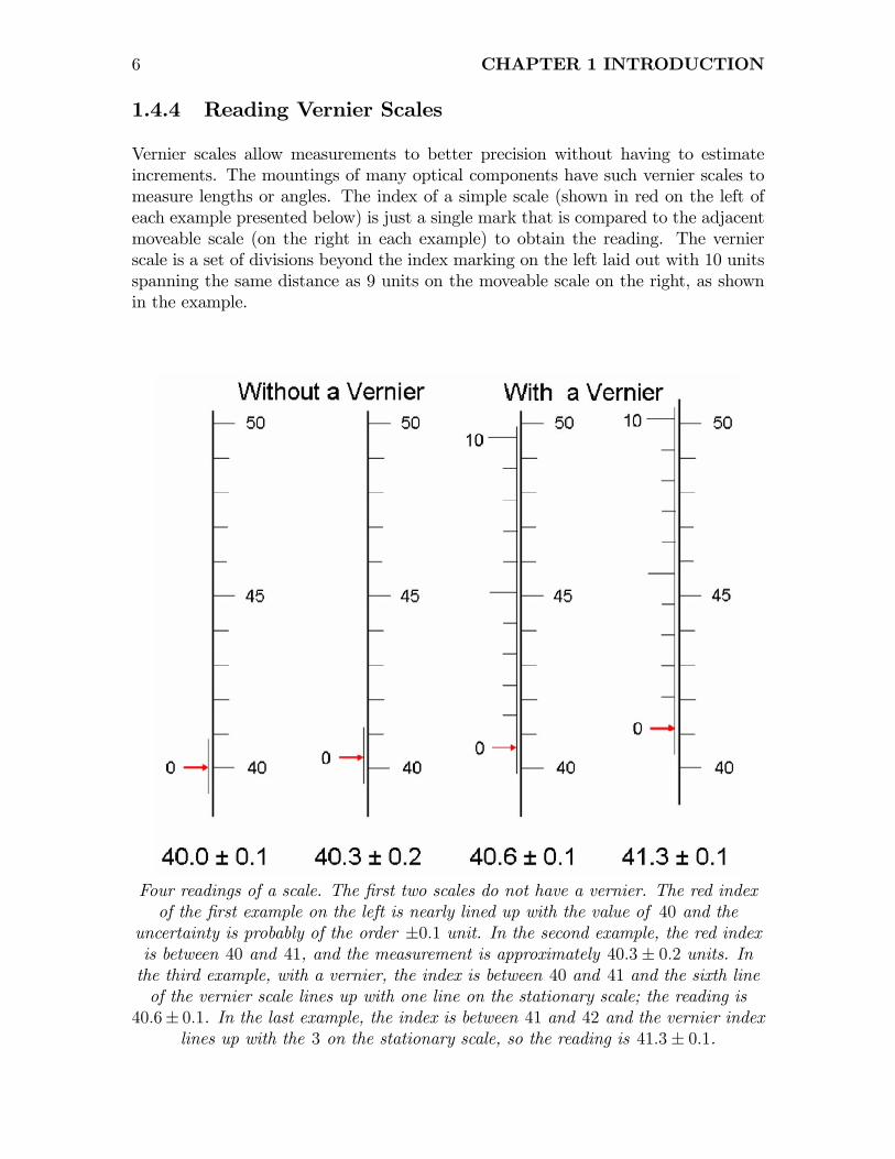
Vernier scales allow measurements to better precision without having to estimateincrements. The mountings of many optical components have such vernier scales tomeasure lengths or angles. The index of a simple scale (shown in red on the left ofeach example presented below) is just a single mark that is compared to the adjacentmoveable scale (on the right in each example) to obtain the reading. The vernierscale is a set of divisions beyond the index marking on the left laid out with 10 unitsspanning the same distance as 9 units on the moveable scale on the right, as shownin the example.
Four readings of a scale. The �rst two scales do not have a vernier. The red indexof the �rst example on the left is nearly lined up with the value of 40 and the
uncertainty is probably of the order �0:1 unit. In the second example, the red indexis between 40 and 41, and the measurement is approximately 40:3� 0:2 units. Inthe third example, with a vernier, the index is between 40 and 41 and the sixth lineof the vernier scale lines up with one line on the stationary scale; the reading is
40:6� 0:1. In the last example, the index is between 41 and 42 and the vernier indexlines up with the 3 on the stationary scale, so the reading is 41:3� 0:1.
1.5 PROPAGATION OF UNCERTAINTY (ERROR) 7
1.5 Propagation of Uncertainty (Error)
Even after you have assessed the uncertainty of your measurements, you still need toestimate the uncertainty of any derived results. For example, if your measurementsof �a�is 10 units �1:5 and �b�is 5 units � 0:5, then what is the undercertainty inthe calculation c = a + b? or d = a� b? You should not report precision above andbeyond what is warranted. For example, I often see students report 5+ decimal placesof precision in numbers derived from observations measured with an uncertainty ofmore than 10%. This is ridiculous (to put it mildly!). So the next question to consideris how to propagate uncertainties in measurements within calculations made fromthose measurements. In other words, we need to determine the error in a calculationwhere pairs of measurements with known precisions are added, subtracted, multiplied,or divided. Suppose that we need to determine a quantity z from other measurements,say x and y via:
z = f [x; y; � � � ]It is generally assumed that the mean value of the quantity z to be determined is thesame function of the mean values of the measured quantities:
�z = f [�x; �y; � � � ]
The uncertainty in z may be evaluated by considering the variation in z that resultsfrom combining individual measurements xn and yn via:
zn = f [xn; yn; � � � ]
The variance in the measurement of z is:
�2z = limN!1
"1
N
NXn=1
(zn � �z)2#
which (clearly) has units of the square of the calculated quantity z. The di¤erenceof the nth calculation of z from the mean �z may be calculated from the di¤erences ofthe individual measurements from their means:
zn � �z �= (xn � �x)@z
@x+ (yn � �y)
@z
@y+ � � �
8 CHAPTER 1 INTRODUCTION
Thus the variance in the calculation is:
�2z�= lim
N!1
"1
N
NXn=1
�(xn � �x)
@z
@x+ (yn � �y)
@z
@y+ � � �
�2#
= limN!1
"1
N
NXn=1
(xn � �x)2�@z
@x
�2#+ limN!1
"+1
N
NXn=1
(yn � �y)2�@z
@y
�2#
+ limN!1
"1
N
NXn=1
2 (xn � �x) (yn � �y)�@z
@x
��@z
@y
�#+ � � �
�2z�= �2x
�@z
@x
�2+ �2y
�@z
@y
�2+ 2�2xy
�@z
@x
��@z
@y
�+ � � �
The error in the calculation of z is the standard deviation �z =p�2z and has the
same units as z.Now consider the speci�c cases that are faced in calculations made from data in
experiments.
1.5.1 Error of a Summation or Di¤erence
If the desired measurement z is the weighted sum of two measurements ax� by, thenthe partial derivatives are:
@z
@x= a
@z
@x= �b
and the resulting variance is:
�2z�= �2x
�@z
@x
�2+ �2y
�@z
@y
�2� 2ab�2xy
= a2�2x + (�b)2 �2y + 2 (+a) (�b) � �2xy
= a2�2x + b2�2y � 2ab � �2xy
=) �z =qa2�2x + b
2�2y � 2ab � �2xy
Example:
For example, consider the calculation of the perimeter of a quadrilateral shape withsides x and y from measurements of two sides; the perimeter is:
z = 2x+ 2y
1.5 PROPAGATION OF UNCERTAINTY (ERROR) 9
The derivatives are:
@z
@x= 2
@z
@y= 2
and the variance in the calculation is:
�2z = �2x
�@z
@x
�2+ �2y
�@z
@y
�2+ 2�2xy
�@z
@x
��@z
@y
�= 22�2x + 2
2�2y + 2 � 2 � 2�2xy = 4��2x + �
2y
�If the measurement of x is 100mm�1mm and that of y = 1000mm�10mm, thenthe perimeter is:
z = 2 � 100mm+2 � 1000mm = 2200mmThe standard deviation in the calculation is:
�z =
q4 � (�1mm)2 + 4 � (�10mm)2 �= 20:1mm
so we speak of the calculation as:
z = 2200mm�20:1mm
What if the error in the measurement of y is the same as that in the measurement ofx? Then the standard deviation is:
�z =
q4 � (�1mm)2 + 4 � (�1mm)2 = 2
p2mm �= 2:83mm
z = 2200mm�2:83mm
If the perimeter is calculated from measurments of the four sides individually, eachwith standard deviation of 1mm:
z = x1 + x2 + y1 + y2
The variance in the measurement is:
�2z = 12 � �2x1 + 1
2 � �2x2 + 12 � �2y1 + 1
2 � �2y2= (1mm)2 + (1mm)2 + (1mm)2 + (1mm)2 = 4mm2
�z =p4mm2 �= 2mm
So the calculation is:z = 2200mm�2:0mm
and the error is less than that in the calculation of the perimeter from measurementsof two sides.
10 CHAPTER 1 INTRODUCTION
1.5.2 Error of a Product or Ratio
If the computation is the scaled product of the two measurements x and y, e.g.,
z = �a � x � y
@z
@x= �a � y
@z
@y= �a � x
�2z = �2x (�a � y)
2 + �2y (�a � x)2 + 2 (�a � y) (�a � x)�2xy
= a2y2�2x + a2x2�2y + 2a
2xy�2xy
= a2�y2�2x + x
2�2y + 2xy�2xy
��2z =
�a2x2y2
� �2xx2+�a2x2y2
� �2yy2+ 2
�a2x2y2
� �2xyxy
=) �2zz2=�2xx2+�2yy2+ 2
�2xyxy
If the computation is the ratio of the two measurements:
z = �axy
=) @z
@x= �a
y
=) @z
@y= �ax
y2
�2z = �2x
��ay
�2+ �2y
��axy2
�2+ 2�2xy
��ay
���axy2
�= �2x
a2
y2+ �2y
a2x2
y4� 2�2xy
a2x
y3
=�2xx2
�a2x2
y2
�+
��2yy2a2x2y2
y4
�� 2
�2xyxy
a2x2
y2
=�2xx2�z2�+�2yy2�z2�� 2
�2xyxy
�z2�
=) �2zz2=�2xx2+�2yy2� 2
�2xyxy
1.5 PROPAGATION OF UNCERTAINTY (ERROR) 11
Example:
Now consider the area of the quadrilateral used in the last example, where x =100mm�1mm, y = 1000mm�10mm. The calculated area is:
z = x � y = 105mm2
The uncertainty is obtained from:
@z
@x= y
@z
@x= x
�z =qy2�2x + x
2�2y + xy�2xy
=
q(1000mm)2 � (1mm)2 + (100mm)2 � (10mm)2
�= 1414:2mm2
so the calculation is:z = 100; 000mm2�1414:2mm2
If the error in the measurement of y is the same as that of the measurement of x, weobtain:
z = 100; 000mm2�1005:0mm2
1.5.3 Value of a Measurement Raised to a Power
If the calculation is proportional to a measured value raised to a power, such as:
z = ax�b
The derivative of the calculation with respect to the measurement is:
@z
@x= �ab �
�x�b�1
�= �bz
x
and the standard deviation is related by:
�zz= b
�xx
Example:
Consider the error in the area of a circle based on an inaccurate measurement of itsdiamter, say x = 100mm; �x = 5mm. The area is
z = ��x2
�2=�
4� (100mm)2 = 2500�mm2 �= 7854:0mm2
12 CHAPTER 1 INTRODUCTION
which implies that a = � and b = 2. The standard deviation is:
�z = zb ��xb= 2500�mm2 �2 � 5mm
100mm= 250�mm2 = 785:40mm2
so the calculation of the area is:
z = 7854:0mm2�785:40mm2
1.5.4 Problems:
1. Determine the uncertainty in the calculation of z from the measurement x viathe exponential:
z = a�bx
where a and b are constants.
2. Determine the uncertainty in the calculation of z from the measurement x viaa logarithm:
z = z = a log (bx)
where a and b are constants.
Chapter 2
Lab #1: Summation of Waves
2.1 Rationale:
This laboratory (really a virtual lab based on computer software) introduces the con-cepts of harmonic oscillations and the e¤ects that result when multiple harmonicoscillations are superposed (added) in one and two dimensions. The 1-D case illus-trates concepts that are relevant to temporal and spatial coherence, di¤raction, andinterference of electromagnetic radiation, though these more advanced applicationswill not be considered until later in the course. The 2-D case is a generalization ofthe description of oscillations using complex notation; z � a+ ib, where [a; b] are realnumbers and i �
p�1.
A �harmonic�oscillation is composed of a single sinusoidal frequency. Projectionsof 2-D harmonic oscillatory motion onto any radial line through the origin in the 2-Dplane yields examples of 1-D harmonic oscillatory motion which all have the samefrequency and amplitude, and with the initial phase determined by the particularaxis chosen.
2.2 Preparation:
1. Write the general equation for a simple harmonic oscillation in trigonometricform (i.e., as a function of the trigonometric functions sine, cosine, etc.).
2. Draw a diagram of the motion of a harmonic oscillator as a function of time,including a graph of the output as a function of time. Designate on the drawingsthe amplitude, period, angular frequency, phase angle, and initial phase, andspecify the units for each.
2.3 Equipment:
1. Personal Computer running Windows
2. DOS Program �Wave.exe�
13
14 CHAPTER 2 LAB #1: SUMMATION OF WAVES
3. DOS Program �Signals.exe�, available from http://www.cis.rit.edu/resources/software
4. Windows Program �Audacity.exe�, available from http://audacity.sourceforge.net/
2.4 Procedure:
The lab utilizes two (ancient, but still serviceable) DOS programs: Wave.exe andSignals.exe. The �rst was written by Taek Gyu Kim, a former graduate student inImaging Science, and allows both 1-D and 2-D sinusoids to be added and displayeddynamically. Roger Easton wrote the second program to demonstrate signal process-ing operations and allows summations and products of various signals to be computedeasily and displayed in various graphical formats.Note that if you run these programs in the WINDOWS environment, the graphics
screens can be captured to the clipboard and pasted into WINDOWS applicationprograms (such as WORDTM or POWERPOINTTM). This capability is useful whendoing lab writeups. The image of a graphics screen may be captured to the WIN-DOWS Clipboard by pressing simultaneously the �ALT� and �PRINT SCREEN�keys. Once captured, the graphics screen may be copied into a WINDOWS applica-tion by pressing the �CTRL�and �V�keys simultaneously when running the desiredapplication. You can toggle between the �full-screen graphics�mode for the DOSprograms and the normal WINDOWS screen by simultaneously pressing �ALT�and�ENTER�. The full WINDOWS screen may be captured to the Clipboard by pressingjust the �PRINT SCREEN�key.The data in Signals.exe also may be exported by using the �spreadsheet�option
�H�in the �Plotting�menu; this creates a three-column �le of spreadsheet data thatcan be imported into such programs as Microsoft ExcelTM. The user is asked to enteran eight-character �le name and the su¢ x �.ssf� is added (for SpreadSheet File).The three columns are the index of the sample, the real part of the data, and theimaginary part of the data.
2.4.1 Summation of 1-D oscillations using Wave.exe
The summation of same-frequency and di¤erent-frequency oscillations will be inves-tigated. To run the program:
1. Start the program by double-clicking on the WAVE icon or by double-clickingon the �lename WAVE.exe, which is located in the SIMG-232 directory.
2. Select the plotting speed (1=slowest,10=fastest); try 5 to start.
3. Select option 2 for linear superposition, where the oscillations are added in onedirection;
4. Select the amplitude A (0 � A � 1), angular frequency ! (listed as �w�on thecomputer), which is measured in units of 2� radians per unit time, and initialphase angle � (in units of �
2radians) for both waves;
2.4 PROCEDURE: 15
5. Sit back and watch the action. The �ESCAPE�key stops the motion and askswhether you wish to continue. Typing n aborts the program, while typing yreturns you to the choice of type of oscillations to add. Note that you cannotrestart the oscillation you were running after typing �ESCAPE�.
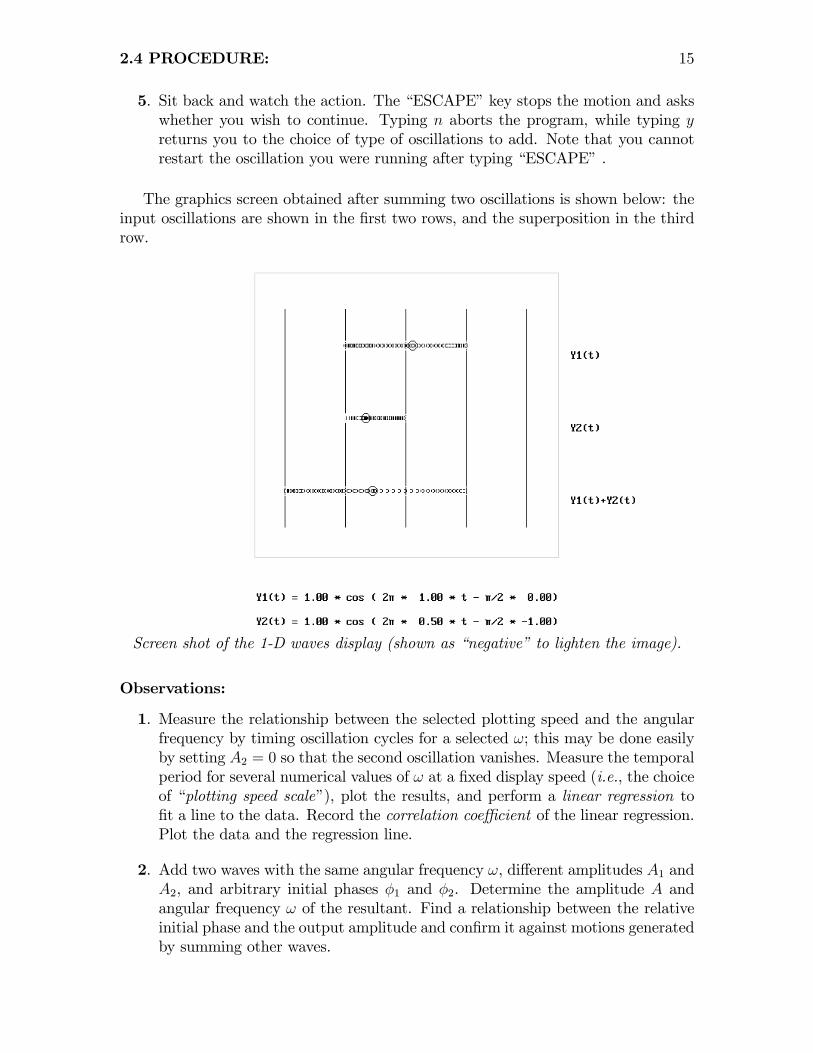
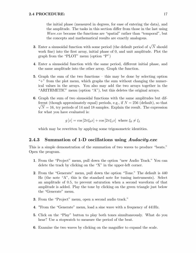
The graphics screen obtained after summing two oscillations is shown below: theinput oscillations are shown in the �rst two rows, and the superposition in the thirdrow.
Screen shot of the 1-D waves display (shown as �negative�to lighten the image).
Observations:
1. Measure the relationship between the selected plotting speed and the angularfrequency by timing oscillation cycles for a selected !; this may be done easilyby setting A2 = 0 so that the second oscillation vanishes. Measure the temporalperiod for several numerical values of ! at a �xed display speed (i.e., the choiceof �plotting speed scale�), plot the results, and perform a linear regression to�t a line to the data. Record the correlation coe¢ cient of the linear regression.Plot the data and the regression line.
2. Add two waves with the same angular frequency !, di¤erent amplitudes A1 andA2, and arbitrary initial phases �1 and �2. Determine the amplitude A andangular frequency ! of the resultant. Find a relationship between the relativeinitial phase and the output amplitude and con�rm it against motions generatedby summing other waves.
16 CHAPTER 2 LAB #1: SUMMATION OF WAVES
3. Add two waves with the same amplitude A1 = A2 and di¤erent (but not very)angular frequencies !1 and !2. The resultant amplitude oscillates as a functionof time in a complicated motion that actually is the sum of a rapidly varyingterm and a slowly varying term. Measure both temporal periods and computethe frequencies. This illustrates the important and common phenomenon of�BEATS�, which appear in may areas of science.
2.4.2 Summation of 1-D oscillations using Signals.exe
The software Signals.exe was written to illustrate concepts of linear systems andFourier transforms, but it also is useful to demonstrate properties of complex numbersand functions, optics, and digital image processing. Both this program and a beta-testWindows version may be downloaded for free from the CIS website at:
http://www.cis.rit.edu/resources/software/
An online User�s Manual is available at:
http://www.cis.rit.edu/resources/software/sig_manual.html
Many di¤erent functions may be entered into the program from the FUNCTIONSmenu (option �F�). The functions are entered as sampled arrays of selectable size(N = 2m for m = 1; 2; : : : ; 13, so that n = 2; 4; 8; : : : ; 8192. There are two arraysavailable: f1 [n] and f2 [n], operate on single functions from the OPERATIONS menu(option �O�), combine two functions from the �ARITHMETIC�menu (option �A�),and graph them from the �PLOT�menu (option �P�).To run the program:
1. Start the program by double-clicking on the SIGNALS icon or by double-clickingon the �lename Signals.exe, which is located in the SIMG-232 directory.
2. Load a function from the FUNCTIONS menu (obtained by typing �F� fromany menu). All functions are loaded in a speci�c sequence:
f [n] = Re ff [n]g �mR [n] + Im ff [n]g �mI [n]
(a) Real Part of the function f [n], Re ff [n]g(b) Modulation of the real part of the function mR [n]
(c) Imaginary Part of the function Im ff [n]g(d) Modulation of the imaginary part mI [n]
Multiple functions may be added at each step, i.e., you can enter a sinu-soidal function and a rectangle function into the real part of the functionto produce the sum of the two. In this section, you will just be enteringthe real part of a sinusoidal function, which is option ��S�in the functionsmenu. The options for the sinusoid are the period (measured in samples),
2.4 PROCEDURE: 17
the initial phase (measured in degrees, for ease of entering the data), andthe amplitude. The tasks in this section di¤er from those in the last usingWave.exe because the functions are �spatial�rather than �temporal�, butthe concepts and mathematical results are exactly analogous.
3. Enter a sinusoidal function with some period (the default period ofpN should
work �ne) into the �rst array, initial phase of 0, and unit amplitude. Plot thegraph from the �PLOT�menu (option �P�)
4. Enter a sinusoidal function with the same period, di¤erent initial phase, andthe same amplitude into the other array. Graph the function.
5. Graph the sum of the two functions � this may be done by selecting option�+�from the plot menu, which graphs the sum without changing the numer-ical values in the arrays. You also may add the two arrays together in the�ARITHMETIC�menu (option �A�), but this deletes the original arrays.
6. Graph the sum of two sinusoidal functions with the same amplitudes but dif-ferent (though approximately equal) periods, e.g., if N = 256 (default), so thatpN = 16, try periods of 14 and 18 samples. Explain the result. The expression
for what you have evaluated is:
g [x] = cos [2��0x] + cos [2��1x] where �0 6= �1
which may be rewritten by applying some trigonometric identities.
2.4.3 Summation of 1-D oscillations using Audacity.exe
This is a simple demonstration of the summation of two waves to produce �beats.�Open the program.
1. From the �Project�menu, pull down the option �new Audio Track.�You candelete the track by clicking on the �X�in the upper-left corner.
2. From the �Generate�menu, pull down the option �Tone.�The default is 440Hz (the note �A�, this is the standard note for tuning instruments). Selectan amplitude of 0:5, to prevent saturation when a second waveform of thatamplitude is added. Play the tone by clicking on the green triangle just belowthe �Generate�menu.
3. From the �Project�menu, open a second audio track.�
4. "From the �Generate�menu, load a sine wave with a frequency of 441Hz.
5. Click on the �Play�button to play both tones simultaneously. What do youhear? Use a stopwatch to measure the period of the beat.
6. Examine the two waves by clicking on the magni�er to expand the scale.
18 CHAPTER 2 LAB #1: SUMMATION OF WAVES
7. Add the two waves; �rst �select all� in the �Edit�menu, then select �QuickMix�in the �Project�menu. This should create a single track that is the sumof both tracks. Expand the scale using the �Magnify� tool to examine thewaveform.
8. Select a section of the sum waveform (say, about 5 s long) and choose �PlotSpectrum�from the �View�menu; this evaluates the FFT of the selection anddisplays the spectrum.
9. Open a new track and generate a square wave of some base frequency. Listento the tone and examine the spectrum. Describe the �quality�of the tone.
10. Open a new track and generate �white noise;�listen to the signal and plot thespectrum. This should demonstrate why the noise is called �white.�
2.4.4 Orthogonal Summation of Oscillations usingWave.exe
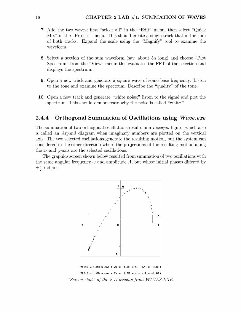
The summation of two orthogonal oscillations results in a Lissajou �gure, which alsois called an Argand diagram when imaginary numbers are plotted on the verticalaxis. The two selected oscillations generate the resulting motion, but the system canconsidered in the other direction where the projections of the resulting motion alongthe x- and y-axis are the selected oscillations.The graphics screen shown below resulted from summation of two oscillations with
the same angular frequency ! and amplitude A, but whose initial phases di¤ered by��2radians.
�Screen shot�of the 2-D display from WAVES.EXE.
2.4 PROCEDURE: 19
1. Add pairs of oscillations to produce: linear vibration along the diagonal, clock-wise and counterclockwise circular motion, and elliptical motion where the ma-jor axis lies along one of the Cartesian axes (x or y), and an ellipse whosemajor axis is at another angle. Also, you are invited to experiment with theparameters to generate other kinds of �gures.
2. If the two oscillations have the same frequency, but arbitrary amplitude andinitial phase, what can you say about the result?
2.4.5 Orthogonal Summation of Functions using Signals.exe
1. First, replicate one of the cases already considered in Part B by entering aCOSINE wave in the real part with a long period (say 128 samples in an arrayof size N = 256) and with initial phase �0 = 0�, and a SINE wave of the sameperiod in the imaginary part (initial phase �0 = �90�).
2. Display the function in the PLOTMenu as real-imaginary parts (option �R�), asmagnitude-phase (option �Q�followed by �U�), and as an ARGAND diagram(option �N�, with other choices to connect the points, draw symbols at thepixels, and use the SLOW display to allow the process to be viewed).
3. Reenter the arrays but change the initial phase of the imaginary part to �0 =+90�. What is the di¤erence in the displayed Argand diagram? We speak ofthe rate of change of the phase angle of the display as the frequency of thecomplex function. In this example, the rate of change of phase is constant, sothe frequency is �xed.
4. Reenter the arrays but change the initial phase of the imaginary part to �0 =+45�. What is the di¤erence in the displayed Argand diagram?
5. One at a time, enter new functions in the REAL and IMAGINARY parts andplot the waves:
(a) REAL Part: SINUSOID (option �S� in the �FUNCTIONS�menu) withperiod = 64, amplitude = 1, center pixel = 0, initial phase = 0�, IMAGI-NARY Part: SINUSOID with period = 64, amplitude = 1
2, center pixel =
0, and initial phase = �90�:(b) REAL Part: SINUSOID (option �S� in the �FUNCTIONS�menu) with
period = 64, amplitude = 1, center pixel = 0, initial phase = 0�, IMAGI-NARY Part: SINUSOID with period = 48, amplitude = 1, center pixel =0, and initial phase = �90�:
(c) REAL Part: SINUSOID (option �S� in the �FUNCTIONS�menu) withperiod = 64, amplitude = 1, center pixel = 0, initial phase = 0�, IMAGI-NARY Part: SINUSOID with period = 64, amplitude = 1, center pixel =0, and initial phase = �45�:
20 CHAPTER 2 LAB #1: SUMMATION OF WAVES
(d) REAL Part: SINUSOID (option �S� in the �FUNCTIONS�menu) withperiod = 64, amplitude = 1, center pixel = 0, initial phase = 0�, IMAGI-NARY Part: SINUSOID with period = 64, amplitude = 1, center pixel =0, and initial phase = �135�:
(e) REAL Part: CHIRP function (option �C�in the �FUNCTIONS�menu)with period = 64, amplitude = 1, center pixel = 0, and initial phase = 0�,IMAGINARY Part: CHIRP with period = 64, amplitude = 1, center pixel= 0, and initial phase = �90�: What is di¤erent about the �frequency�ofthis function compared to that where the REAL and IMAGINARY partsare sinusoidal functions?
6. In all cases, view the results as real-imaginary parts (option �R�in the �PLOT�menu), as magnitude/phase (option �M�or option �U�followed by �Q�in the�PLOT�menu) and as the ARGAND diagram (option �N� in the �PLOT�menu).
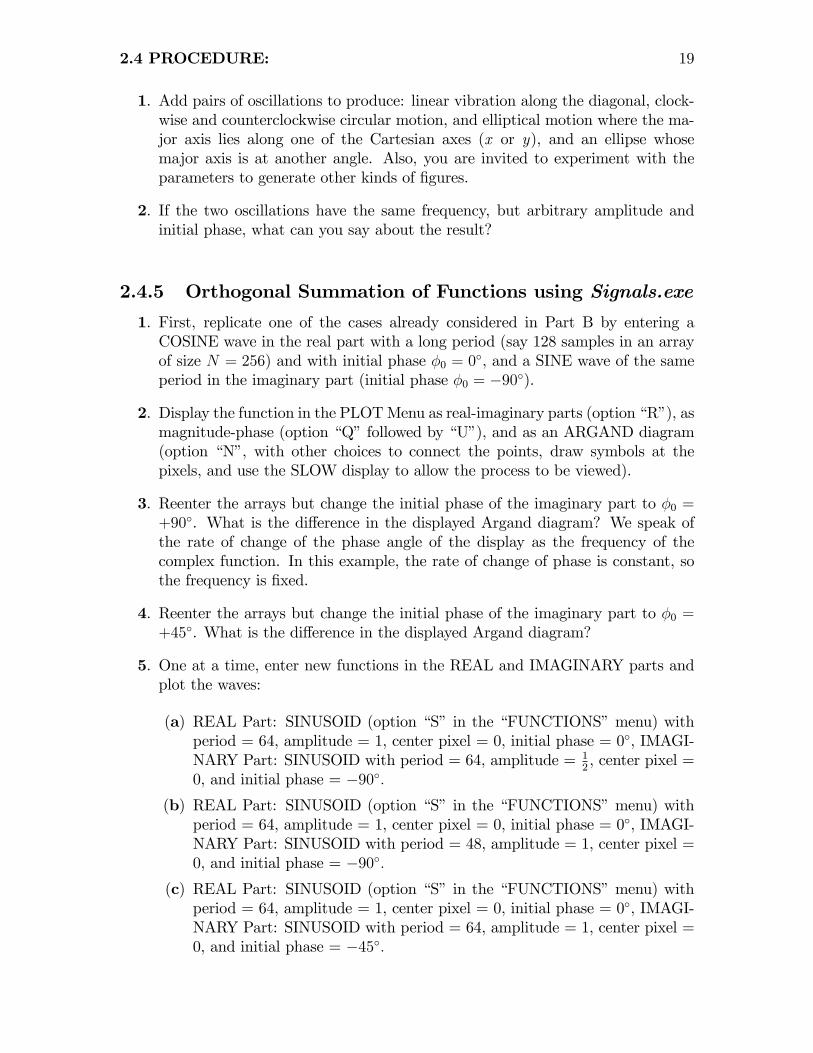
7. Repeat the procedure for a few other functions (your choice). For example, entersinusoids of equal amplitudes and a phase di¤erence of �90�, and modulate thefunction by multiplying the entire function by a decaying function such as anegative exponential. View the Argand diagram (option �N� in the �PLOT�menu).
�Screen shot�of Argand diagram in �SIGNALS.EXE�
2.4.6 Nonlinear Operations on Sinusoidal Waves in Signals
In all of the steps thus far, the output has been the a single wave or the summationof two or more sinusoidal waves. In this section, we brie�y consider the result of aspeci�c �nonlinear�operation on a wave.
2.4 PROCEDURE: 21
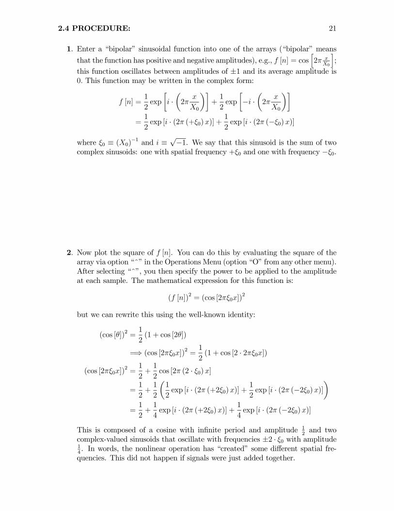
1. Enter a �bipolar� sinusoidal function into one of the arrays (�bipolar�meansthat the function has positive and negative amplitudes), e.g., f [n] = cos
h2� x
X0
i;
this function oscillates between amplitudes of �1 and its average amplitude is0: This function may be written in the complex form:
f [n] =1
2exp
�i ��2�
x
X0
��+1
2exp
��i �
�2�
x
X0
��=1
2exp [i � (2� (+�0)x)] +
1
2exp [i � (2� (��0)x)]
where �0 � (X0)�1 and i �
p�1. We say that this sinusoid is the sum of two
complex sinusoids: one with spatial frequency +�0 and one with frequency ��0.
2. Now plot the square of f [n]. You can do this by evaluating the square of thearray via option �^�in the Operations Menu (option �O�from any other menu).After selecting �^�, you then specify the power to be applied to the amplitudeat each sample. The mathematical expression for this function is:
(f [n])2 = (cos [2��0x])2
but we can rewrite this using the well-known identity:
(cos [�])2 =1
2(1 + cos [2�])
=) (cos [2��0x])2 =
1
2(1 + cos [2 � 2��0x])
(cos [2��0x])2 =
1
2+1
2cos [2� (2 � �0)x]
=1
2+1
2
�1
2exp [i � (2� (+2�0)x)] +
1
2exp [i � (2� (�2�0)x)]
�=1
2+1
4exp [i � (2� (+2�0)x)] +
1
4exp [i � (2� (�2�0)x)]
This is composed of a cosine with in�nite period and amplitude 12and two
complex-valued sinusoids that oscillate with frequencies �2 � �0 with amplitude14. In words, the nonlinear operation has �created�some di¤erent spatial fre-quencies. This did not happen if signals were just added together.
22 CHAPTER 2 LAB #1: SUMMATION OF WAVES
2.5 Questions:
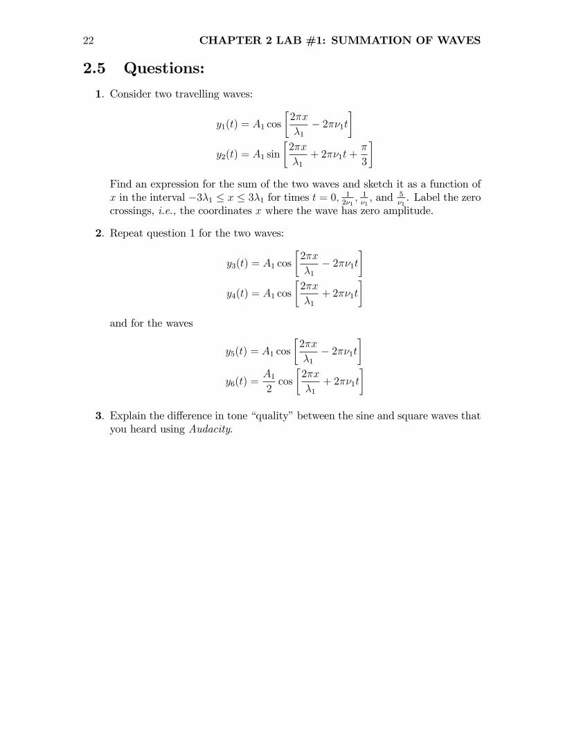
1. Consider two travelling waves:
y1(t) = A1 cos
�2�x
�1� 2��1t
�y2(t) = A1 sin
�2�x
�1+ 2��1t+
�
3
�Find an expression for the sum of the two waves and sketch it as a function ofx in the interval �3�1 � x � 3�1 for times t = 0; 1
2�1; 1�1, and 5
�1. Label the zero
crossings, i.e., the coordinates x where the wave has zero amplitude.
2. Repeat question 1 for the two waves:
y3(t) = A1 cos
�2�x
�1� 2��1t
�y4(t) = A1 cos
�2�x
�1+ 2��1t
�and for the waves
y5(t) = A1 cos
�2�x
�1� 2��1t
�y6(t) =
A12cos
�2�x
�1+ 2��1t
�3. Explain the di¤erence in tone �quality�between the sine and square waves thatyou heard using Audacity.
Chapter 3
Lab #2: Dispersion
3.1 References:
Physical Optics, Robert W. Wood, Optical Society, 1988 (reprint of book originallypublished in 1911)Waves, Frank Crawford, Berkeley Physics Series, McGraw-Hill, 1968.The Nature of Light, V. Ronchi, Harvard University Press, 1970.Rainbows, Haloes, and Glories, Robert Greenler, Cambridge University Press,
1980.Sunsets, Twilights, and Evening Skies, Aden and Marjorie Meinel, Cambridge
University Press, 1983.Light and Color in the Outdoors, M.G.J. Minnaert, Springer-Verlag, 1993.
3.2 Rationale:
Many optical imaging systems used for scienti�c purposes (e.g., in remote sensingor astronomy) generate images from light collected in relatively narrow bands ofwavelengths. Three common choices exist for �splitting�the light into its constituentwavelengths. The simplest is by inserting �bandpass��lters into the light path thatpass light in only narrow selected bands (you will use such �lters in part of thislab). The second method uses an optical element formed from a periodic pattern oftransparent and opaque regions. This �grating�forces di¤erent wavelengths to travelalong paths at angles proportional to the wavelength. The third method, which isthe subject of this lab, also �disperses�the light, but uses the physical mechanism ofdi¤erential refraction due to the inherent property that di¤erent wavelengths travelat di¤erent speeds in glass.
3.3 Theory:
From the study of refraction in geometrical optics, we know that light rays incident onan interface between two transparent materials are refracted at an angle determined
23

24 CHAPTER 3 LAB #2: DISPERSION
by the incident angle and by the phase velocities of light in the two materials. Theratio of the phase velocity of light in vacuum to that in a material is the refractiveindex n:
n =c
vwhere c = 3 � 108m
s. The �phase velocity�v in the medium is the ratio of the angular
frequency ! and the �wavenumber�k, which is equal to the product of the wavelength� and the temporal frequency �:
v =!
k= � � �
By combining the two equations, we obtain an expression for the refractive index interms of the vacuum velocity c, the angular frequency !, and the wavenumber k.
n = c ��k
!
�Snell�s law relates the indices of refraction to the angles of light rays in two media.If the angles of the incident and refracted rays are �1 and �2, respectively (measuredfrom the vector normal to the surface), then Snell�s law is:
n1 sin [�1] = n2 sin [�2]
A plot of the e¤ect on an incident ray is shown in Figure 1:
Illustration of Snell�s Law.
Elementary discussions of refraction often assume that the indices of refraction donot vary with the temporal frequency � of the light. For real materials, the situation ismore complicated. Obviously, the phase velocity of light waves is slower in a materialthan in vacuum, because n � 1 (except for a few very special cases, such as refractionof x-rays in some materials). But waves with di¤erent � travel at di¤erent velocitiesin media; long waves travel faster than short waves, except over very narrow rangescentered about very speci�c wavelengths (the resonances), which are beyond the scope

3.3 THEORY: 25
of this laboratory. Therefore, n is smaller for longer waves than for shorter. A plot ofthe refractive indices of several media vs. wavelength, i.e., a plot of n [�] for severalmedia, is shown in Figure 2.
Refractive Index n vs. Wavelength � for several media. Note that n decreases withincreasing �, which means that the velocity of light in the medium increases with
increasing �.
White light can be dispersed into its constituent frequencies (or equivalently, itswavelength spectrum) by utilizing this di¤erential velocity of light in materials com-bined with Snell�s law. The intensity of the dispersed light can be measured andplotted as a spectrum, which is a valuable tool for determining the chemical con-stituents of the light source or an intervening medium. In fact, spectral imaging(forming images of objects in narrow wavebands of light) has become a hot topicin imaging because of advances in dispersing materials, computer technologies, andprocessing algorithms.The best-known method for dispersing light is based on di¤erential refraction
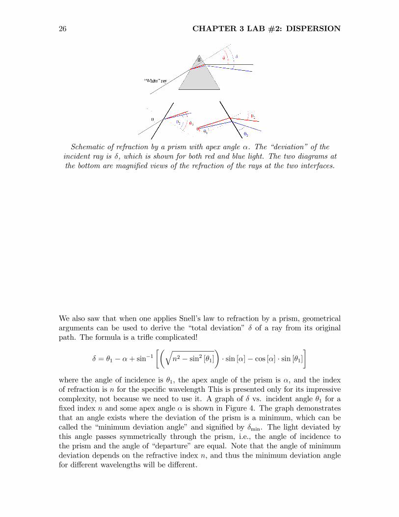
within a block of glass with �at sides fabricated at an angle (usually 60� but otherangles are common). Of course, this was the scheme used by Newton to performthe �rst spectral �analysis�of white light (spreading it into its constituent colors) in1671. Note that Newton also �synthesized�white light by recombining the coloredcomponents. Newton was the �rst to investigate the spectral components of white andcolored light, and in this way was arguably the �rst to perform a Fourier analysis.Newton did make a famous error in this study by assuming that the e¤ect of thedispersion was proportional to the refractive index of the glass. In other words,he assumed that the dispersion is a property of the index and does not di¤er withmaterial.Consider a prism with apex angle � shown in Figure 3. A light ray is incident at
angle �1.
26 CHAPTER 3 LAB #2: DISPERSION
Schematic of refraction by a prism with apex angle �. The �deviation�of theincident ray is �, which is shown for both red and blue light. The two diagrams atthe bottom are magni�ed views of the refraction of the rays at the two interfaces.
We also saw that when one applies Snell�s law to refraction by a prism, geometricalarguments can be used to derive the �total deviation� � of a ray from its originalpath. The formula is a tri�e complicated!
� = �1 � �+ sin�1��q
n2 � sin2 [�1]�� sin [�]� cos [�] � sin [�1]
�where the angle of incidence is �1, the apex angle of the prism is �, and the indexof refraction is n for the speci�c wavelength This is presented only for its impressivecomplexity, not because we need to use it. A graph of � vs. incident angle �1 for a�xed index n and some apex angle � is shown in Figure 4. The graph demonstratesthat an angle exists where the deviation of the prism is a minimum, which can becalled the �minimum deviation angle�and signi�ed by �min. The light deviated bythis angle passes symmetrically through the prism, i.e., the angle of incidence tothe prism and the angle of �departure�are equal. Note that the angle of minimumdeviation depends on the refractive index n, and thus the minimum deviation anglefor di¤erent wavelengths will be di¤erent.
3.4 EQUIPMENT: 27
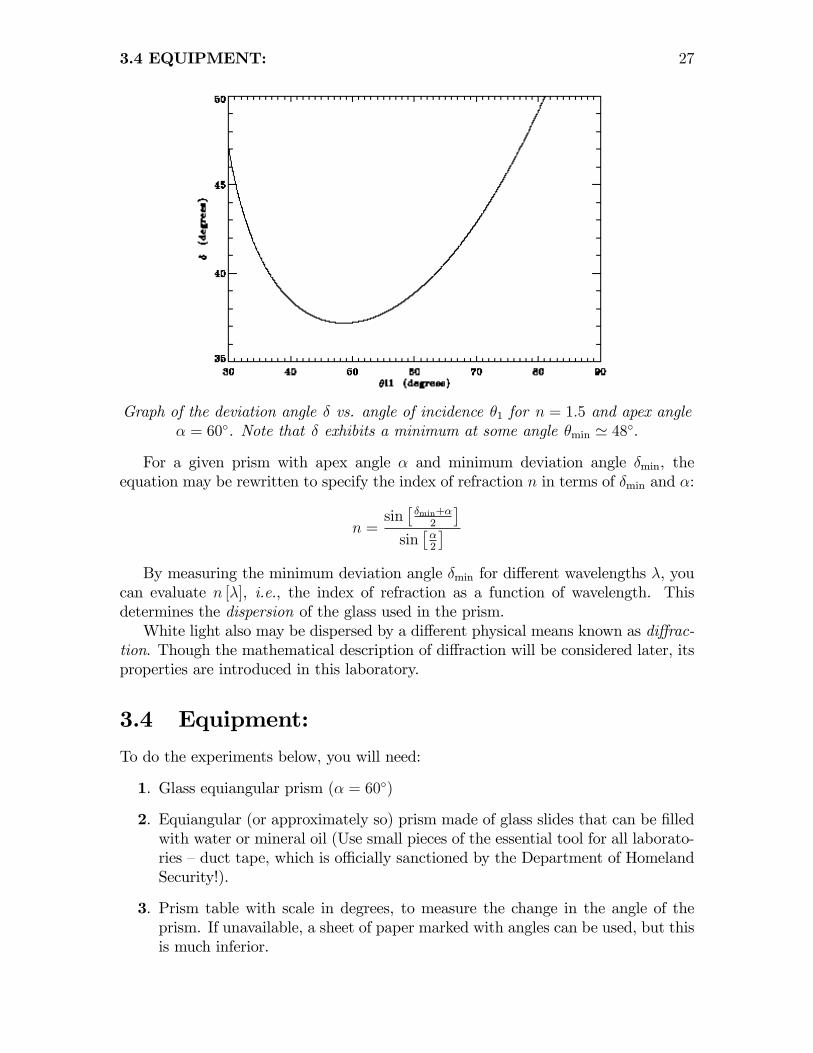
Graph of the deviation angle � vs. angle of incidence �1 for n = 1:5 and apex angle� = 60�. Note that � exhibits a minimum at some angle �min ' 48�.
For a given prism with apex angle � and minimum deviation angle �min, theequation may be rewritten to specify the index of refraction n in terms of �min and �:
n =sin��min+�
2
�sin��2
�By measuring the minimum deviation angle �min for di¤erent wavelengths �, you
can evaluate n [�], i.e., the index of refraction as a function of wavelength. Thisdetermines the dispersion of the glass used in the prism.White light also may be dispersed by a di¤erent physical means known as di¤rac-
tion. Though the mathematical description of di¤raction will be considered later, itsproperties are introduced in this laboratory.
3.4 Equipment:
To do the experiments below, you will need:
1. Glass equiangular prism (� = 60�)
2. Equiangular (or approximately so) prism made of glass slides that can be �lledwith water or mineral oil (Use small pieces of the essential tool for all laborato-ries �duct tape, which is o¢ cially sanctioned by the Department of HomelandSecurity!).
3. Prism table with scale in degrees, to measure the change in the angle of theprism. If unavailable, a sheet of paper marked with angles can be used, but thisis much inferior.
28 CHAPTER 3 LAB #2: DISPERSION
4. He:Ne laser
5. White-light source with optical �ber output
6. Colored �lters made of glass or gelatin (�gels�)
7. Aluminum foil (to make slits to reduce the spreading of the light passed intothe prism).
8. Di¤raction grating(s)
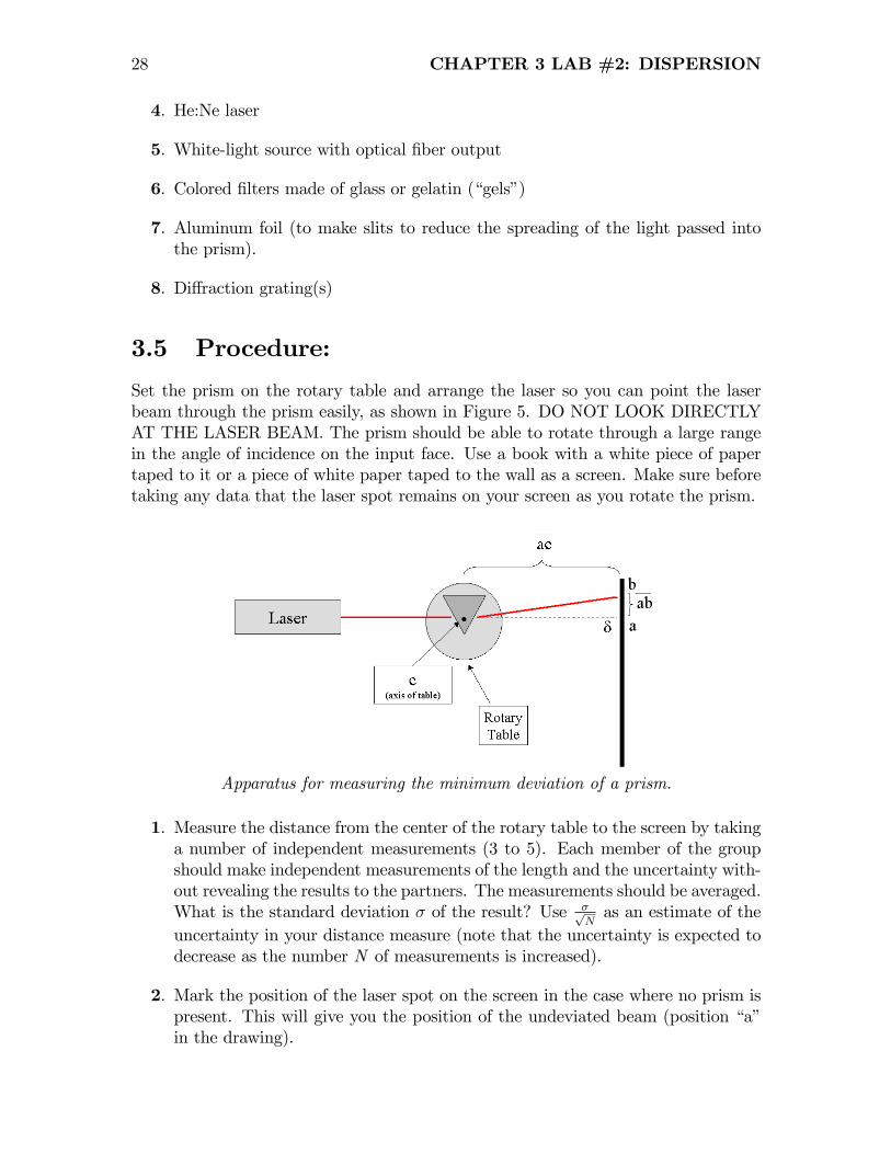
3.5 Procedure:
Set the prism on the rotary table and arrange the laser so you can point the laserbeam through the prism easily, as shown in Figure 5. DO NOT LOOK DIRECTLYAT THE LASER BEAM. The prism should be able to rotate through a large rangein the angle of incidence on the input face. Use a book with a white piece of papertaped to it or a piece of white paper taped to the wall as a screen. Make sure beforetaking any data that the laser spot remains on your screen as you rotate the prism.
Apparatus for measuring the minimum deviation of a prism.
1. Measure the distance from the center of the rotary table to the screen by takinga number of independent measurements (3 to 5). Each member of the groupshould make independent measurements of the length and the uncertainty with-out revealing the results to the partners. The measurements should be averaged.What is the standard deviation � of the result? Use �p
Nas an estimate of the
uncertainty in your distance measure (note that the uncertainty is expected todecrease as the number N of measurements is increased).
2. Mark the position of the laser spot on the screen in the case where no prism ispresent. This will give you the position of the undeviated beam (position �a�in the drawing).

3.5 PROCEDURE: 29
3. Measure the apex angle of the glass prism supplied. You can draw lines par-allel to the faces of the prism, extend these lines with a ruler, and then use aprotractor to make the measurement.
4. Place the prism in the center of the rotary table or angle sheet. Find the positionwhere the re�ected beam travels directly back to the laser source; this is thelocation where the face of the prism is perpendicular to the laser beam. Rotatethe prism until you see a spot of laser light that has been refracted by the prism.Mark the position of the laser spot for di¤erent incident angles for as large arange of angles and of spot positions as you can measure. Take at least 8 datapoints, recording the value of the incident angle (as judged by the position ofthe rotary table) and the distance from the undeviated spot position.
5. Convert the distances from the previous step to deviation angles � [�1]. Thiscan be done by noting that:
ab
ac= tan [�]
where ab is the distance from a to b in �gure and ac is the distance from a toc, both of which you have measured.
6. Hold the water prism up to your eye and look at "things" (lamps and such)with it. You should see colored edges around white lamps or objects; this iscalled chromatic aberration in lenses. Cover a small white light source with agelatin �lter and look at the light through the water prism; a purple �lter workswell, as it transmits red and blue light while blocking green. (Crawford, #4.12p.217)
7. Now remove your glass prism and �ll the hollow prismmade from the microscopeslides with the distilled water provided. Repeat steps 1 through 5. Obviously,you cannot mount this prism vertically, so this is a more subjective experiment.But try to estimate the di¤erence in the deviation between the water and glassprisms.
8. Repeat steps 1-5 after �lling the microscope-slide prism with a liquid, such aswater or mineral oil (or both).
9. Go back to the glass prism and use an optical �ber light source and a slit insteadof the laser. Put the �ber source at least a couple of feet away from the prism.Make a slit that is a few millimeters wide and about 10mm long. Measure theangle of incidence as best you can, and then measure the deviation � for threedi¤erent colors: red, green (or yellow), and blue. If you have trouble, you maywant to consider holding �lters from the optics kit in front of the slit to cut outthe unwanted colors. In any case, you will probably have to turn the lights o¤and shield your screen from the ambient light to be able to see the slit on yourscreen.
30 CHAPTER 3 LAB #2: DISPERSION
10. Now, replace the prism with a di¤raction grating and describe the spectrumof the white light. Note particularly the di¤erences compared to the spectrumgenerated by the prism. Sketch approximate paths of light emerging from thegrating, and carefully note the di¤erences in path for red and blue light. Ifavailable, compare the spectrum obtained from di¤raction gratings with di¤er-ent rulings (spacings).
3.6 Analysis:
In your lab write-up, be sure to complete the following:
1. For each of the three prisms, graph the deviation angle � as a function of theincident angle on the input face of the prism, �1. Find the minimum deviationangle, �min and estimate the uncertainty in this quantity.
2. Using the equation, calculate the index of refraction for the glass, water, andmineral oil used, based on your value for�min and � in each case.
3. From your measurements, derive the index of refraction for red (� ' 700 nm),green (� ' 550 nm) and blue (� ' 550 nm) light. Do your data show an decreasein n with increasing wavelength? The laser is also red (� ' 632:8 nm). Howwell does your value of n agree between the laser measurements and the red�lter measurement?
3.7 Questions:
1. Imagine that a source emits a pulse of light 1 �s long which is composed ofequal amplitudes of all wavelengths. The light is incident on a block of glass ofthickness 20 km and whose refractive index as shown above.
(a) What is the physical length of the pulse [m] when the light enters the glass?
(b) What is the time required for red light and for blue light to traverse theglass?
(c) What is the physical length of the pulse emerging from the glass.
(d) Describe the �color�of the emerging pulse.
2. If the dispersion of the glass is as shown in the plot of refractive index, and ifthe light is incident on the equiangular prism at the angle shown, determineand sketch approximate paths followed by red light (� = 600 nm) and by bluelight (� = 400 nm) and �nd the approximate di¤erence in emerging angle (the�dispersion angle�, often denoted by �). Sketch the path of the light fromincidence through the glass to the emergence. Note carefully which color isdeviated more.
3.7 QUESTIONS: 31
3. Sketch the path followed by the light if it is incident from within a block of thesame type of glass onto a �prism-shaped�hole.
4. Describe the relative values of the velocity of the average wave and the mod-ulation wave for if the material has the dispersion curve shown. What if thedispersion curve is reversed (i.e., if nred > nblue)?
5. Now that you�ve �nished this lab on dispersion, reconsider the question of theformation process of rainbows. Some answers given at the beginning of thequarter speculated that rainbows were caused by di¤racted or by scatteredsunlight. Recall (either from experience or research) and sketch the relativelocations of the rainbow, the viewer, and the sun. On your sketch, show thepath followed by the di¤erent colors from the sun to the eye. In other words,explain the sequence of colors in the rainbow.
BONUS QUESTION:
6. Find a description of and an explanation for the atmospheric phenomenonknown as the �green �ash�, which is occasionally seen at the �nal instant ofsunset from locations with an unobstructed horizon. Explain why the e¤ect isnot called a �blue �ash�.

Chapter 4
Lab #3: Polarization
4.1 Background:
This lab introduces the concept of polarization of light. As we have said in class(and as is obvious from the name), electromagnetic radiation requires two traveling-wave vector components to propagate: the electric �eld, often speci�ed by E, andthe magnetic �eld B. The two components are orthogonal (perpendicular) to eachother, and mutually orthogonal to the direction of travel, which is often speci�ed bythe vector quantity s (the Poynting vector):
s � E�B
where ���speci�es the mathematical �cross product�.
4.1.1 Cross Product
Just to review, the cross product of two arbitrary three-dimensional vectors a =[ax; ay; az] and b = [bx; by; bz] is de�ned:
a�b � det
26664x y z
ax ay az
bx by bz
37775� x (aybz � byaz) + y (azbx � bzax) + z (axby � aybx)
where x, y, and z are the unit vectors directed along the respective Cartesian axesand det [ ] represents the evaluation of the determinant of the 3� 3 matrix. You mayrecall that the �cross product�is ONLY de�ned for 3-D vectors.For example, if the electric �eld E is oriented along in the x -direction with am-
plitude Ex (so that Ejjx, where jj indicates �is parallel to�). The electric �eld isE = x � Ex + y � 0 + z � 0. Consider also that the magnetic �eld B ? E is orientedalong the y-direction (Bjjy, B = x � 0 + y �By + z � 0), then the electromagnetic �eld
33
34 CHAPTER 4 LAB #3: POLARIZATION
travels in the direction speci�ed by:
E � B � det
26664x y z
Ex 0 0
0 By 0
37775= x (0 � 0�By � 0) + y (Ex � 0� 0 � 0) + z (Ex �By � 0 � 0)= z (Ex �By)
Thus the electromagnetic wave propagates in the direction of the positive z axis.
4.1.2 Polarization
In vacuum (sometimes called free space), the electric and magnetic �elds propagatewith the same phase, e.g., if the electric �eld is a traveling wave with phase k0z �!0t+ �0, then the two component �elds are:
E [z; t] = xE0 cos [k0z � !0t+ �0]
B [z; t] = yB0 cos [k0z � !0t+ �0] = y�E0c
�cos [k0z � !0t+ �0]
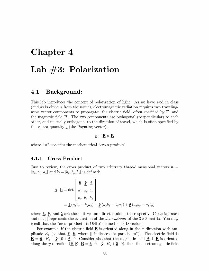
where c is the velocity of light in vacuum. Of course, we know the relationships ofthe wavenumber k0 = 2�=�0, the temporal angular frequency !0 = 2��0 = 2�c=�0,and the velocity c = �0�0. Because the amplitude of the electric �eld is larger by afactor of c, the phenomena associated with the electric �eld are easier to measure.The direction of the electric �eld E (which may vary with time/position) is called thepolarization of the radiation.
For waves in vacuum, the electric and magnetic �elds are �in phase�and the wavetravels in the direction speci�ed by s = E� B.
Polarized light comes in di¤erent �avors: plane (or linear), elliptical, and circular.In the �rst lab on oscillations, we introduced some of the types of polarized light whenwe added oscillations in the x- and y-directions (then called the real and imaginaryparts) with di¤erent amplitudes and initial phases. The most commonly referencedtype of light is plane polarized, where the electric �eld vector E points in the same
4.1 BACKGROUND: 35
direction for di¤erent points in the wave. Plane-polarized waves with E oriented alongthe x- or y-axis are easy to visualize; just construct a traveling wave oriented alongthat direction. Plane-polarized waves at an arbitrary angle � may be constructedby adding x- and y-components with the same frequency and phase and di¤erentamplitudes, e.g.,
E [z; t] = xEx cos [k0z � !0t+ �0] + yEy cos [k0z � !0t+ �0]
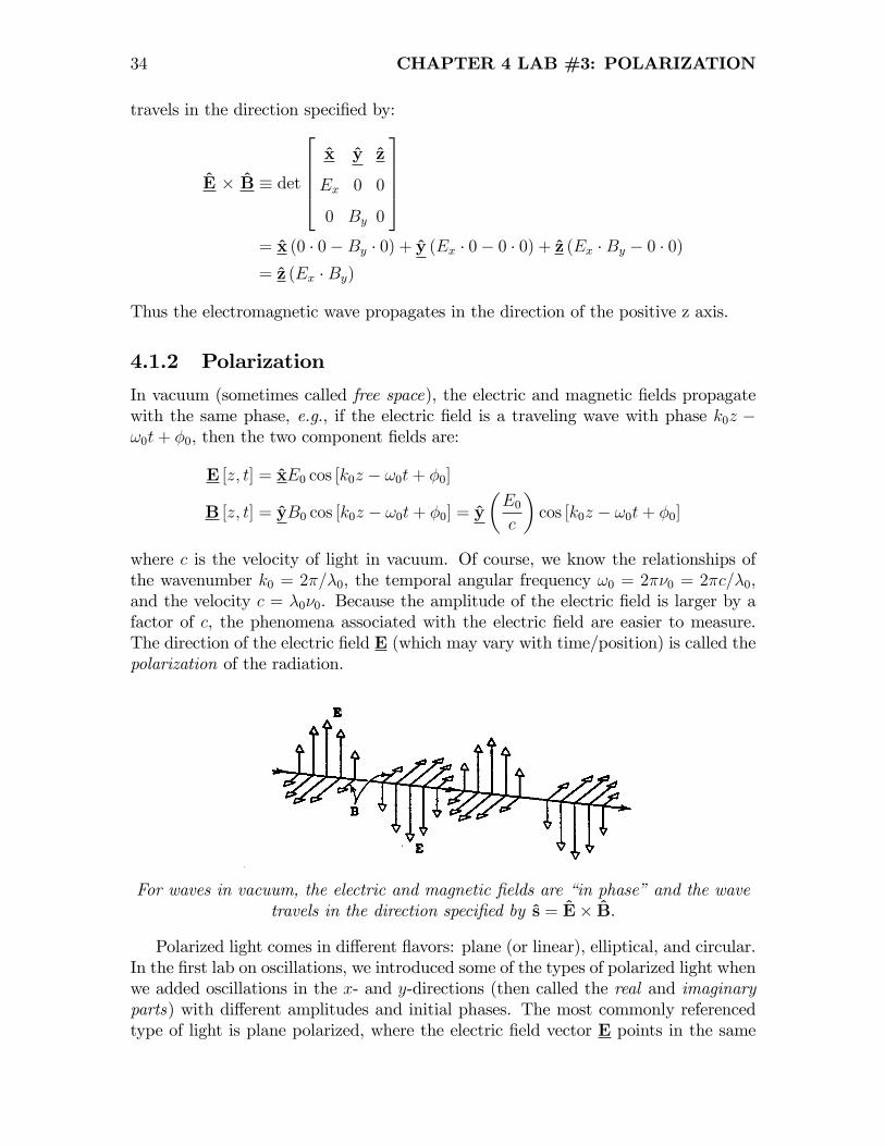
When the two component electric �elds are �in phase�(so that the arguments ofthe two cosines are equal for all [z; t]), then the angle of polarization, speci�ed by �,is obtained by a formula analogous to that for the phase of a complex number:
� = tan�1�Ey cos [k0z � !0t+ �0]Ex cos [k0z � !0t+ �0]
�= tan�1
�EyEx
�as shown in Figure 2.
Angle of linear polarization for (Ex)max = 1 and (Ey)max = 0:5 is
tan=1hEyEx
i�= 0:463 radians �= 26:6�.
Note that the electric �elds directed along the x- and y-directions are independent;they need not have the same amplitude, frequency, or initial phase. In this discussionof polarization, the components must have the same frequency, but may have di¤erentamplitudes (as just shown) and/or initial phases. If the amplitudes are equal to E0but the initial phases di¤er by �=2 radians, we have:
E [z; t] = E0
�x cos [k0z � !0t+ �0] + y cos
hk0z � !0t+ �0 �
�
2
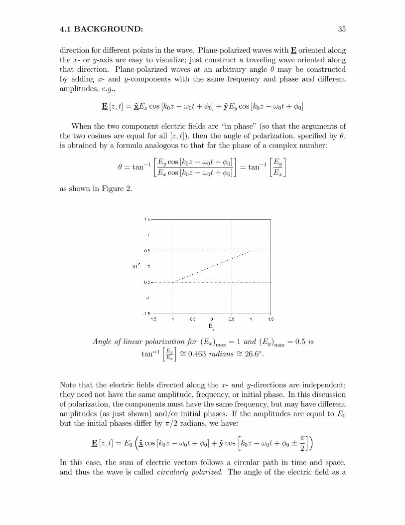
i�In this case, the sum of electric vectors follows a circular path in time and space,and thus the wave is called circularly polarized. The angle of the electric �eld as a
36 CHAPTER 4 LAB #3: POLARIZATION
Figure 4.1: Propagation of circularly polarized light: the phase of Ey is delayed (oradvanced) by �
2radians relative to Ex.
function of [z; t] may be evaluated:
� = � [z; t] = tan�1
"E0 cos
�k0z � !0t+ �0 � �
2
�E0 cos [k0z � !0t+ �0]
#= tan�1
"cos�k0z � !0t+ �0 � �
2
�cos [k0z � !0t+ �0]
#
= tan�1�� sin [k0z � !0t+ �0]cos [k0z � !0t+ �0]
�= tan�1 [� tan [k0z � !0t+ �0]] = � [k0z � !0t+ �0]
In words, the angle of the electric vector is a linear function of z and of t; the angleof the electric vector changes with time and space.
You may want to reexamine or redo that experiment. A similar con�gurationwhere the amplitudes in the x- and y-directions are not equal is called ellipticallypolarized.
Circularly polarized light may be generated by delaying the phase of one com-ponent of plane-polarized light by �=2 radians, or 1/4 of a period. The device forintroducing the phase delay is called a quarter-wave plate. We can also construct ahalf-wave plate such that the output wave is:
E [z; t] = E0�x cos [k0z � !0t+ �0] + y cos [k0z � !0t+ �0 � �]
�= E0
�x cos [k0z � !0t+ �0] + y (� cos [k0z � !0t+ �0])
�= E0
�x� y
�cos [k0z � !0t+ �0]
4.2 EQUIPMENT: 37
� = � [z; t] = tan�1��E0 cos [k0z � !0t+ �0]E0 cos [k0z � !0t+ �0]
�= tan�1 [�1] = ��
4
4.1.3 Nomenclature for Circular Polarization
Like linearly polarized light, circularly polarized light has two orthogonal states, i.e.,clockwise and counterclockwise rotation of the E-vector. These are termed right-handed (RHCP) and left-handed (LHCP). There are two conventions for the nomen-clature:
1. Angular MomentumConvention (my preference): Point the thumb of the
8<: rightleft
9=;hand in the direction of propagation. If the �ngers point in the direction of ro-
tation of the E-vector, then the light is
8<: RHCPLHCP
9=; :2. Optics (also called the �screwy�) Convention: The path traveled by the E-vector of RHCP light is the same path described by a right-hand screw. Ofcourse, the natural laws de�ned by Murphy ensure that the two conventions areopposite: RHCP light by the angular momentum convention is LHCP by thescrew convention.
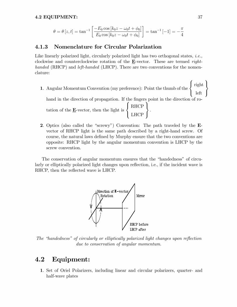
The conservation of angular momentum ensures that the �handedness�of circu-larly or elliptically polarized light changes upon re�ection, i.e., if the incident wave isRHCP, then the re�ected wave is LHCP.
The �handedness�of circularly or elliptically polarized light changes upon re�ectiondue to conservation of angular momentum.
4.2 Equipment:
1. Set of Oriel Polarizers, including linear and circular polarizers, quarter- andhalf-wave plates
38 CHAPTER 4 LAB #3: POLARIZATION
2. He:Ne laser
3. Fiber-optic light source
4. Radiometer (light meter)
5. Optical rail + carriers to hold polarizers, etc.
6. One rotatable stage to hold polarizer at measurable azimuth angle measuredfrom vertical
7. Saran WrapTM or Handi-WrapTM: stretchy wrap used for sandwiches
4.3 Procedure:
This lab consists of several sections:
1. an investigation of plane-polarized light, including a measurement of the inten-sity of light after passing through two polarizers oriented at a relative angle of�
2. an investigation of Malus�law for plane-polarized light.
3. a mechanism for generating plane-polarized light by re�ection,
4. an investigation of circularly polarized light, and
5. a demonstration of polarization created by scattering of the electric �eld by airmolecules.
Your lab kit includes linear and circular polarizers, and quarter-wave and half-wave plates.
1. Plane-Polarized Light: the common mechanism for generating polarized lightfrom unpolarized light is a ��lter�that removes any light with electric vectorsoriented perpendicular to the desired direction. This is the device used incommon polarized sunglasses.
(a) Orient two polarizers in orthogonal directions and look at the transmittedlight.
(b) Add a third polarizer AFTER the �rst two so that it is oriented at anangle of approximately �=4 radians (45�) and note the result.
(c) Add a third polarizer BETWEEN the �rst two so that it is oriented at anangle of approximately �=4 radians and note the result.
4.3 PROCEDURE: 39
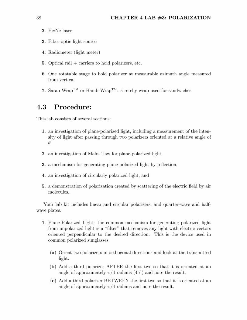
2. Malus�Law (Figure 5) This experiment uses laser sources, and a few wordsof warning are necessary: NEVER LOOK DIRECTLY AT A LASERSOURCE THE INTENSITY IN THE BEAM IS VERY CONCEN-TRATED AND CAN DAMAGE YOUR RETINA
Setup for con�rming Malus�Law
(a) Mount a screen behind polarizer P1 and test the radiation from the laserto see if it is plane polarized and, if so, at what angle.
(b) Measure the �baseline�intensity of the source using the CCD camera (withlens). You may have to attenuate the light source with a piece of paperand/or stop down the aperture of the lens.
(c) Insert one polarizer in front of the detector and measure the intensityrelative to the original un�ltered light. How much light does one polarizerlet through? Next, increase the intensity of the light until you nearly geta saturated image on the CCD.
(d) Add a second polarizer to the path and orient it �rst to maximize andthen to minimize the intensity of the transmitted light. Measure bothintensities.
(e) Next we will try to con�rm Malus�Law. Two polarizers must again beused: one to create linearly polarized light, and one to �test�for the po-larization. The second polarizer often is called an analyzer, and if possible,use one of the rotatable polarizers on the optical mounts. Set up the po-larizers and adjust the light intensity so that when they are aligned, theimage on the camera is again nearly saturated.
(f) Measure the transmitted light for di¤erent relative angles (say, every 10�
or so) by rotating the second polarizer. �Grab� an image of the sourcethrough the two polarizers and determine the average pixel value for yourlight source at each angle. Plot the data graphically as a function of angleand compare to Malus�law:
3. Polarization by re�ection (Figure 6):
(a) Look at the re�ection of light from a glossy surface (such as re�ections ofthe ceiling lights from a waxed �oor or the smooth top of a desk) through
40 CHAPTER 4 LAB #3: POLARIZATION
the polarizer. Rotate the polarizer to �nd the direction of greatest trans-mission. This indicates the direction of linear polarization that is trans-mitted by the polarizer. If possible, document the re�ection at di¤erentangles by a photograph with a digital camera through the polarizer.
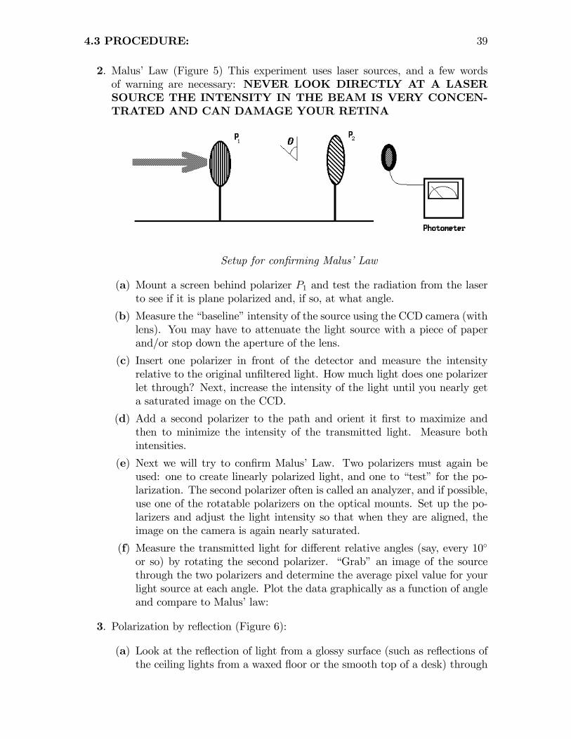
(b) Use a setup shown so that the laser beam re�ects from a glass prism; theprism just serves as a piece of glass with a �at surface and not for dispersionor internal re�ection. Place one of the linear polarizers between the laserand the �rst mirror. Focus your attention on the intensity of the beamre�ected from the front surface of the prism �you probably will need todarken the room.
(c) Rotate the prism on the paper sheet with angular markings to vary theincident angle �i. At each �i, rotate the polarizer to minimize the trans-mitted intensity. At a particular �i, the intensity of the transmitted beamshould be essentially zero. This angle �i of minimum re�ection is Brew-ster�s angle, where the electric-�eld vector parallel to the plane of incidenceis not re�ected. Measure Brewster�s angle at least 4 times and average toget your �nal result.
(d) Remove the polarizer from the incident beam and use it to examine thestate of polarization of the re�ected light.
Setup for measuring polarization by re�ection.
4. Circular Polarization: as stated above, circularly polarized light is generatedby delaying (or advancing) the phase of one component of linearly polarizedlight by 90� with a quarter-wave plate. A circular polarizer can be constructedfrom a sandwich of a linear polarizer and a quarter-wave plate. In this way, thecircular polarizer is sensitive to the direction of propagation of the light.
(a) Construct a circular polarizer with the components available and test itby laying it on a shiny surface (a coin works well). Shine a light sourceon the arrangement from above, and test the behavior as you rotate thelinear polarizer. Make sure you can see a variation in intensity of the lightre�ected by the coin. You should be able to see one clear minimum inintensity between 0 and 90�.
4.4 ANALYSIS: 41
(b) Orient your CCD camera so you can grab images of the coin at di¤erentorientation angles. Measure the intensity at several (�= 7) di¤erent anglesfrom 0 to 90 degrees, including one near the minimum intensity.
5. Make a quarter-wave plate from several (6 or 7) layers of sandwich wrap bytaping the wrapping to a piece of cardboard with a hole cut in it. This isconvenient because it can be �tuned� to speci�c colors of light by adding orsubtracting layers (more layers for longer �).. Test to see if this actually actsas a quarter-wave plate by using it to make a circular polarizer and testing there�ection from a shiny coin.
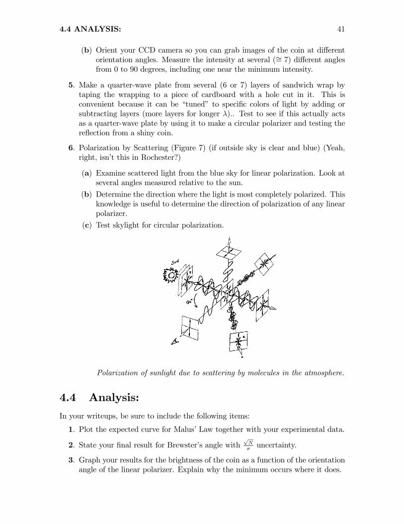
6. Polarization by Scattering (Figure 7) (if outside sky is clear and blue) (Yeah,right, isn�t this in Rochester?)
(a) Examine scattered light from the blue sky for linear polarization. Look atseveral angles measured relative to the sun.
(b) Determine the direction where the light is most completely polarized. Thisknowledge is useful to determine the direction of polarization of any linearpolarizer.
(c) Test skylight for circular polarization.
Polarization of sunlight due to scattering by molecules in the atmosphere.
4.4 Analysis:
In your writeups, be sure to include the following items:
1. Plot the expected curve for Malus�Law together with your experimental data.
2. State your �nal result for Brewster�s angle withpN�uncertainty.
3. Graph your results for the brightness of the coin as a function of the orientationangle of the linear polarizer. Explain why the minimum occurs where it does.
42 CHAPTER 4 LAB #3: POLARIZATION
4.5 Questions:
1. Consider why sunglasses used while driving are usually made with polarizedlenses. Determine the direction of polarization of the �lters in sunglasses. Theprocedure to determine the direction of polarization of light re�ected from aglossy surface or by scattering from molecules are helpful.
2. Explain the action of the circular polarizer on re�ection.
3. Considered the circular polarizer you constructed. If the angle of the plane(linear) polarizer is not correct, what will be the character of the emerginglight?

Chapter 5
Lab #4: Division-of-WavefrontInterference
5.1 Theory
Recent labs on optical imaging systems have used the concept of light as a �ray�in geo-metrical optics to model the action of lenses. We were able to determine the locationsof images and their magni�cations. However, the concept of light as a �wave�alsois fundamental to imaging, particularly in its manifestation in �di¤raction�, which isthe fundamental limitation on the action of an optical imaging system. �Interference�and �di¤raction�may be interpreted as the same phenomenon, di¤ering only in thenumber of sources involved (interference =) few sources, say 2 - 10; di¤raction =)many sources, up to an in�nite number). In this lab, the two sources are obtained bydividing the wave emitted by a single source by introducing two apertures into thesystem; this is called �division of wavefront�. In the next lab, we will divide the lightby introducing a beamsplitter to create �division-of-amplitude interferometry�.
5.1.1 Interference:
We introduce interference by recalling the expression for the sum of two sinusoidaltemporal oscillations of the same amplitude and di¤erent frequencies:
A cos [!1t] + cos [!2t] = 2A cos
�(!1 + !2)
2t
�cos
�(!1 � !2)
2t
�= 2A cos [!modt] cos [!avgt]
and the travelling-wave analogue:for two plane waves propagating along the z axis:
A cos [k1z � !1t] + A cos [k2z � !2t] = 2A cos [kmodz � !modt] cos [kavgz � !avgt]
kmod =k1 � k22
; !mod =!1 � !22
; kavg =k1 + k22
; !avg =!1 + !22
43
44CHAPTER 5 LAB#4: DIVISION-OF-WAVEFRONT INTERFERENCE
If the dispersion is normal, the resulting wave is the product of a slow traveling wavewith velocity vmod =
!modkmod
and a rapid traveling wave with velocity vavg =!avgkavg
. Thusfar, we have described traveling waves directed along one axis (usually z). Of course,the equations can be generalized easily to model waves traveling in any direction.Instead of a scalar angular wavenumber k, we can de�ne the 3-D wavevector :
k = [kx; ky; kz] = xkx + yky + zkz
which points in the direction of travel of the wave. The length of the wavevectoris proportional to ��1.
jkj =qk2x + k
2y + k
2z =
2�
�:
Thus the equation for a traveling wave in 3-D space becomes:
f [x; y; z; t] = f [r; t] = A cos [kxx+ kyy + kzz � !t] = A cos [k�r� !t]
For simplicity, we will limit ourselves to the 2-D case, where the equation of awave is:
f [x; y; t] = A cos [kxx+ kyy � !t] = A cos [k�r� !t]
A 2-D or 3-D wavefront can exhibit a periodic variation in the phase � [r; t] =k�r� !t, even if !1 = !2 = ! ! �1 = �2 = �. If light from a single source is dividedinto two sections by introducing two apertures into the system, Huygens�principleindicates that the light through the two apertures will �spread�and recombine. Whenviewed at a single location, the two �beams�of light with the same wavelength willrecombine with di¤erent wavevectors such that jk1j = jk2j = jkj. This happens whenthe Cartesian sum of the components of k are the same, but
[(kx)1; (ky)1] 6= [(kx)2; (ky)2]
Note that the following simple result is true only for
�1 = �2:
Light of the same wavelength (and same optical frequency) is described as coherent. Inthis case, consider the superposition of two plane waves of the same optical frequency!, one traveling in direction k1 and one in direction k2:
f1 [x; y; z; t] = A cos [k1�r� !t]f2 [x; y; z; t] = A cos [k2�r� !t] ;
where k1 = [0; ky; kz] and k2 = [0;�ky; kz]; i.e., the wavevectors di¤er only in the signof the y-component. The wavevectors have the same length:
jk1j = jk2j =2�
�=) �1 = �2 � �:
5.1 THEORY 45
The components of the wavevectors are:
kz = jkj cos [�] =2�
�cos [�]
ky =2�
�sin [�] :
The superposition of the electric �elds is:
f1 [x; y; z; t] + f2 [x; y; z; t] = A fcos [(kzz � !t) + kyy] + cos [(kzz � !t)� kyy]g
which can be recast using the formula for cos [�� �] to:
f1 [x; y; z; t] + f2 [x; y; z; t] = 2A cos [kyy] cos [kz � !t]
= 2A cos
��2�
�sin [�]
�y
�cos [kzz � !t]
Note that there is no time dependence in the �rst term: this is a time-invariantpattern. Also recall that the measured quantity is the intensity of the pattern, whichis the time average of the squared magnitude. The time-invariant term thus becomesthe visible pattern:
jf1 [x; y; z; t] + f2 [x; y; z; t] j2 / 4A2 cos2�2�y
�sin [�]
�= 4A2 � 1
2
�1 + cos
�4�y
�sin [�]
��1 [y]
/ 2A2 cos�2�y
D
�, where D � �
2 � sin [�]
where the identity cos2 [�] = 12(1 + cos [2�]) has been used. The intensity pattern has
a cosine form (maximum at the center) and a period proportional to � and inverselyproportional to sin [�]. If � is small, the periodD of the pattern is long. If the distanceL to the observation plane is large, then sin [�] �= d
Land the period of the pattern is
approximately:
D �=�L
d! Dd ' L�
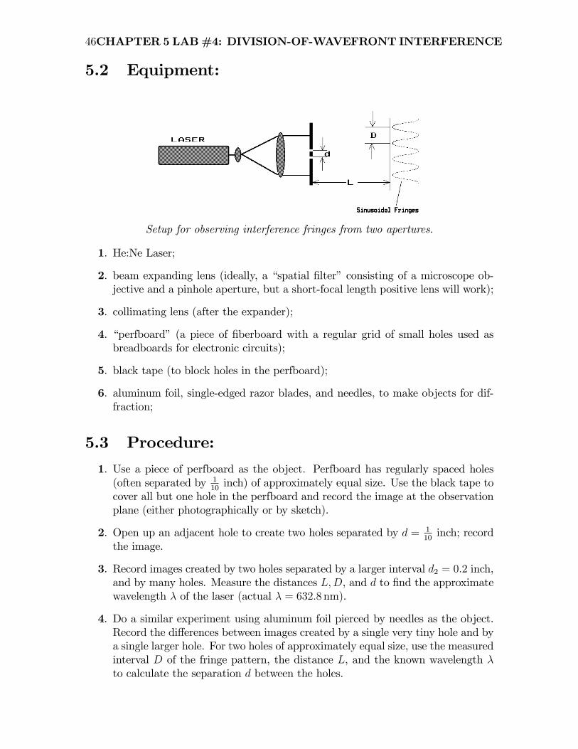
46CHAPTER 5 LAB#4: DIVISION-OF-WAVEFRONT INTERFERENCE
5.2 Equipment:
Setup for observing interference fringes from two apertures.
1. He:Ne Laser;
2. beam expanding lens (ideally, a �spatial �lter�consisting of a microscope ob-jective and a pinhole aperture, but a short-focal length positive lens will work);
3. collimating lens (after the expander);
4. �perfboard� (a piece of �berboard with a regular grid of small holes used asbreadboards for electronic circuits);
5. black tape (to block holes in the perfboard);
6. aluminum foil, single-edged razor blades, and needles, to make objects for dif-fraction;
5.3 Procedure:
1. Use a piece of perfboard as the object. Perfboard has regularly spaced holes(often separated by 1
10inch) of approximately equal size. Use the black tape to
cover all but one hole in the perfboard and record the image at the observationplane (either photographically or by sketch).
2. Open up an adjacent hole to create two holes separated by d = 110inch; record
the image.
3. Record images created by two holes separated by a larger interval d2 = 0:2 inch,and by many holes. Measure the distances L;D, and d to �nd the approximatewavelength � of the laser (actual � = 632:8 nm).
4. Do a similar experiment using aluminum foil pierced by needles as the object.Record the di¤erences between images created by a single very tiny hole and bya single larger hole. For two holes of approximately equal size, use the measuredinterval D of the fringe pattern, the distance L, and the known wavelength �to calculate the separation d between the holes.
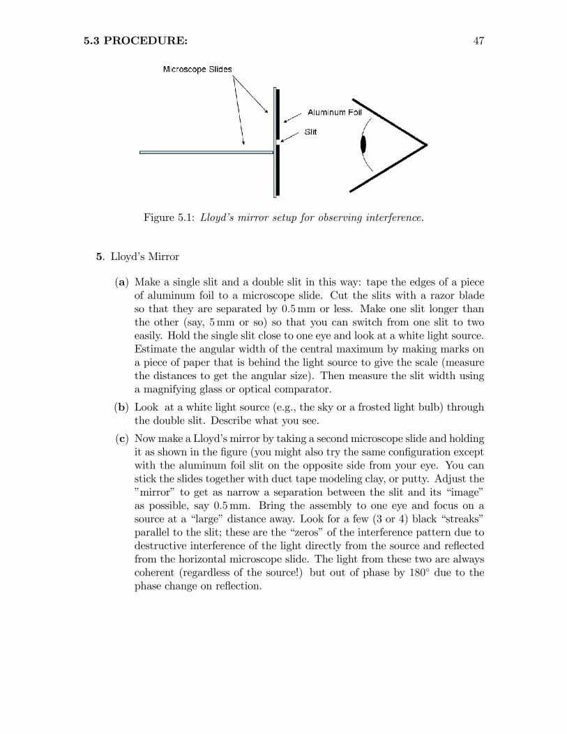
5.3 PROCEDURE: 47
Figure 5.1: Lloyd�s mirror setup for observing interference.
5. Lloyd�s Mirror
(a) Make a single slit and a double slit in this way: tape the edges of a pieceof aluminum foil to a microscope slide. Cut the slits with a razor bladeso that they are separated by 0:5mm or less. Make one slit longer thanthe other (say, 5mm or so) so that you can switch from one slit to twoeasily. Hold the single slit close to one eye and look at a white light source.Estimate the angular width of the central maximum by making marks ona piece of paper that is behind the light source to give the scale (measurethe distances to get the angular size). Then measure the slit width usinga magnifying glass or optical comparator.
(b) Look at a white light source (e.g., the sky or a frosted light bulb) throughthe double slit. Describe what you see.
(c) Nowmake a Lloyd�s mirror by taking a second microscope slide and holdingit as shown in the �gure (you might also try the same con�guration exceptwith the aluminum foil slit on the opposite side from your eye. You canstick the slides together with duct tape modeling clay, or putty. Adjust the�mirror� to get as narrow a separation between the slit and its �image�as possible, say 0:5mm. Bring the assembly to one eye and focus on asource at a �large�distance away. Look for a few (3 or 4) black �streaks�parallel to the slit; these are the �zeros�of the interference pattern due todestructive interference of the light directly from the source and re�ectedfrom the horizontal microscope slide. The light from these two are alwayscoherent (regardless of the source!) but out of phase by 180� due to thephase change on re�ection.

Chapter 6
Lab #5: Division-of-AmplitudeInterference
6.1 Theory:
6.1.1 Division-of-Wavefront Interferometry
In the last lab, you saw that coherent (single-wavelength) light from point sources twodi¤erent locations in an optical beam could be combined after having traveled alongtwo di¤erent paths. The recombined light exhibited sinusoidal fringes whose spatialfrequency depended on the di¤erence in angle of the light beams when recombined.The regular variation in relative phase of the light beams resulted in constructiveinterference (when the relative phase di¤erence is 2�n, where n is an integer) anddestructive interference where the relative phase di¤erence is 2�n+�. The centers ofthe �bright�fringes occur where the optical paths di¤er by an integer multiple of �0.
49
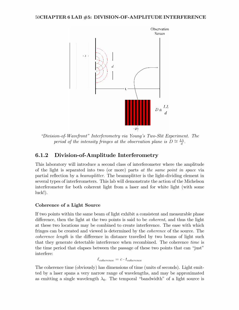
50CHAPTER 6 LAB#5: DIVISION-OF-AMPLITUDE INTERFERENCE
�Division-of-Wavefront�Interferometry via Young�s Two-Slit Experiment. Theperiod of the intensity fringes at the observation plane is D �= L�
d:
6.1.2 Division-of-Amplitude Interferometry
This laboratory will introduce a second class of interferometer where the amplitudeof the light is separated into two (or more) parts at the same point in space viapartial re�ection by a beamsplitter. The beamsplitter is the light-dividing element inseveral types of interferometers. This lab will demonstrate the action of the Michelsoninterferometer for both coherent light from a laser and for white light (with someluck!).
Coherence of a Light Source
If two points within the same beam of light exhibit a consistent and measurable phasedi¤erence, then the light at the two points is said to be coherent, and thus the lightat these two locations may be combined to create interference. The ease with whichfringes can be created and viewed is determined by the coherence of the source. Thecoherence length is the di¤erence in distance travelled by two beams of light suchthat they generate detectable interference when recombined. The coherence time isthe time period that elapses between the passage of these two points that can �just�interfere:
`coherence = c � tcoherenceThe coherence time (obviously) has dimensions of time (units of seconds). Light emit-ted by a laser spans a very narrow range of wavelengths, and may be approximatedas emitting a single wavelength �0. The temporal �bandwidth�of a light source is
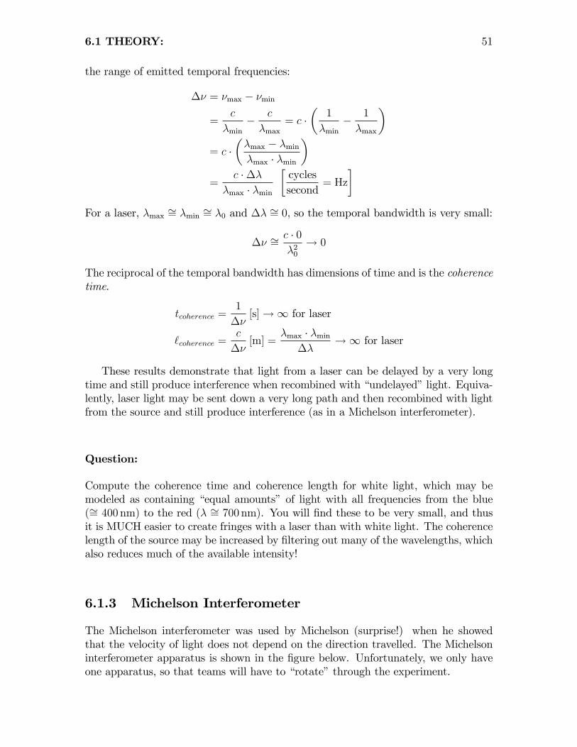
6.1 THEORY: 51
the range of emitted temporal frequencies:
�� = �max � �min
=c
�min� c
�max= c �
�1
�min� 1
�max
�= c �
��max � �min�max � �min
�=
c ����max � �min
�cyclessecond
= Hz
�For a laser, �max �= �min �= �0 and �� �= 0, so the temporal bandwidth is very small:
�� �=c � 0�20
! 0
The reciprocal of the temporal bandwidth has dimensions of time and is the coherencetime.
tcoherence =1
��[s]!1 for laser
`coherence =c
��[m] =
�max � �min��
!1 for laser
These results demonstrate that light from a laser can be delayed by a very longtime and still produce interference when recombined with �undelayed�light. Equiva-lently, laser light may be sent down a very long path and then recombined with lightfrom the source and still produce interference (as in a Michelson interferometer).
Question:
Compute the coherence time and coherence length for white light, which may bemodeled as containing �equal amounts� of light with all frequencies from the blue(�= 400 nm) to the red (� �= 700 nm). You will �nd these to be very small, and thusit is MUCH easier to create fringes with a laser than with white light. The coherencelength of the source may be increased by �ltering out many of the wavelengths, whichalso reduces much of the available intensity!
6.1.3 Michelson Interferometer
The Michelson interferometer was used by Michelson (surprise!) when he showedthat the velocity of light does not depend on the direction travelled. The Michelsoninterferometer apparatus is shown in the �gure below. Unfortunately, we only haveone apparatus, so that teams will have to �rotate�through the experiment.

52CHAPTER 6 LAB#5: DIVISION-OF-AMPLITUDE INTERFERENCE
Collimated Laser Light
The light is split into two beams by the beamsplitter, which is half-silvered on theinside so that light is re�ected after being transmitted through the glass. The twobeams emerging from the beam splitter travel perpendicular paths to mirrors wherethey are directed back to be recombined at the beamsplitter surface. One mirror canbe tilted by an adjustable mirror and the length of the other path may be changed by atranslatable mirror. A compensator (a plain piece of glass of the same thickness as thebeamsplitter) is placed in the beam that was transmitted by beamsplitter. The lighttransits the compensator twice, and thus the path length traveled in glass by lightin this arm is identical to that traveled in glass in the other arm. This equalizationof the path length traveled simpli�es (somewhat) the use of the interferometer witha broad-band white-light source. The compensator is not necessary when a laser isused, because the coherence length is much longer than the path-length di¤erence.
Michelson interferometer using He:Ne laser for illumination (�0 = 632:8 nm).
If the translatable mirror is displaced so that the two beams travel di¤erent dis-tances from the beamsplitter to the mirror (say `1 and `2), then the total optical pathof each beam is 2 � `1 and 2 � `2. The total optical path di¤erence is:
OPD = 2 � `1 � 2 � `2 = 2 ��` [m]
Note that the path length is changed by TWICE the translation distance of the mirror.The OPDmay be scaled to be measured in number of wavelengths of di¤erence simplyby dividing by the laser wavelength:
OPD =2 ��`�0
[wavelengths]
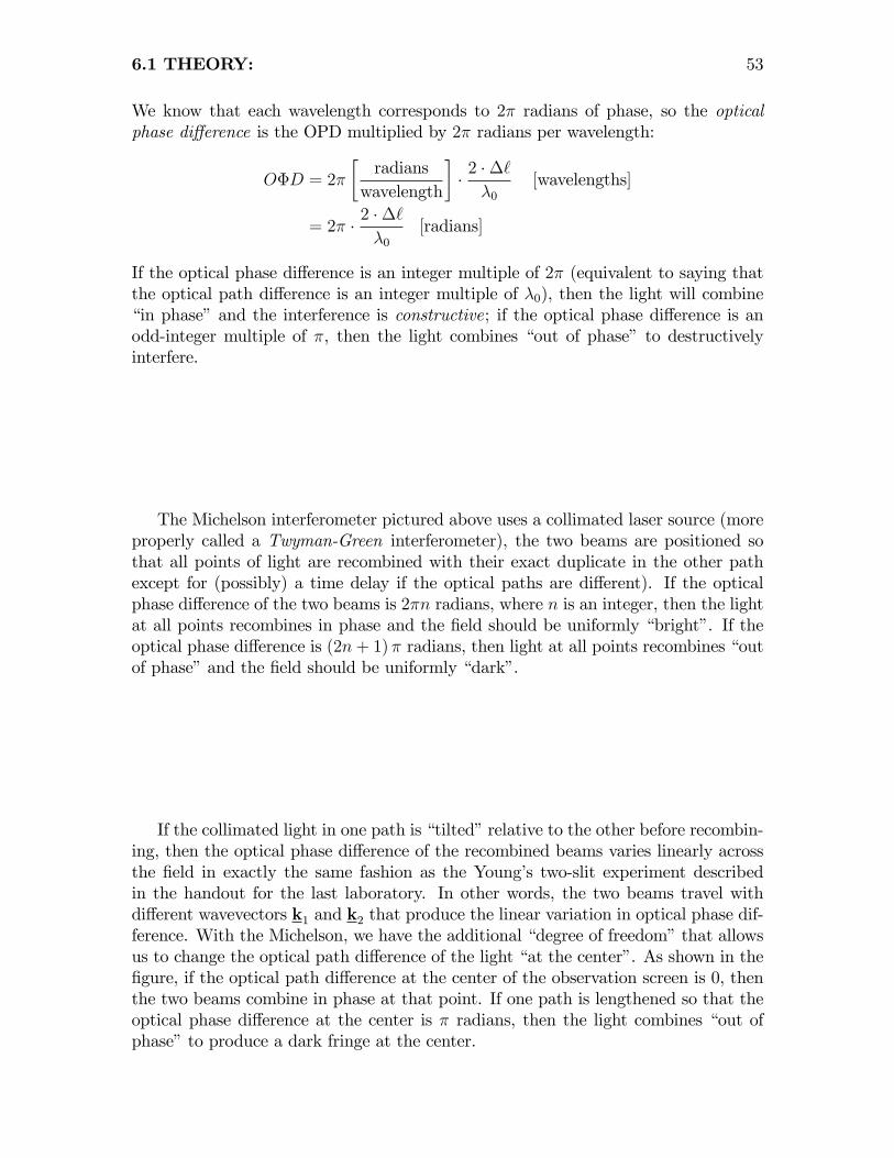
6.1 THEORY: 53
We know that each wavelength corresponds to 2� radians of phase, so the opticalphase di¤erence is the OPD multiplied by 2� radians per wavelength:
O�D = 2�
�radians
wavelength
�� 2 ��`�0
[wavelengths]
= 2� � 2 ��`�0
[radians]
If the optical phase di¤erence is an integer multiple of 2� (equivalent to saying thatthe optical path di¤erence is an integer multiple of �0), then the light will combine�in phase�and the interference is constructive; if the optical phase di¤erence is anodd-integer multiple of �, then the light combines �out of phase� to destructivelyinterfere.
The Michelson interferometer pictured above uses a collimated laser source (moreproperly called a Twyman-Green interferometer), the two beams are positioned sothat all points of light are recombined with their exact duplicate in the other pathexcept for (possibly) a time delay if the optical paths are di¤erent). If the opticalphase di¤erence of the two beams is 2�n radians, where n is an integer, then the lightat all points recombines in phase and the �eld should be uniformly �bright�. If theoptical phase di¤erence is (2n+ 1) � radians, then light at all points recombines �outof phase�and the �eld should be uniformly �dark�.
If the collimated light in one path is �tilted�relative to the other before recombin-ing, then the optical phase di¤erence of the recombined beams varies linearly acrossthe �eld in exactly the same fashion as the Young�s two-slit experiment describedin the handout for the last laboratory. In other words, the two beams travel withdi¤erent wavevectors k1 and k2 that produce the linear variation in optical phase dif-ference. With the Michelson, we have the additional �degree of freedom�that allowsus to change the optical path di¤erence of the light �at the center�. As shown in the�gure, if the optical path di¤erence at the center of the observation screen is 0, thenthe two beams combine in phase at that point. If one path is lengthened so that theoptical phase di¤erence at the center is � radians, then the light combines �out ofphase�to produce a dark fringe at the center.
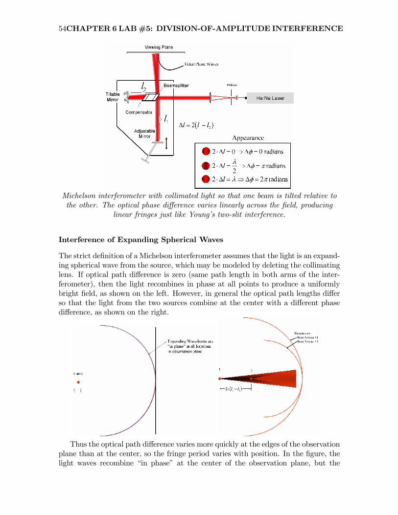
54CHAPTER 6 LAB#5: DIVISION-OF-AMPLITUDE INTERFERENCE
Michelson interferometer with collimated light so that one beam is tilted relative tothe other. The optical phase di¤erence varies linearly across the �eld, producing
linear fringes just like Young�s two-slit interference.
Interference of Expanding Spherical Waves
The strict de�nition of a Michelson interferometer assumes that the light is an expand-ing spherical wave from the source, which may be modeled by deleting the collimatinglens. If optical path di¤erence is zero (same path length in both arms of the inter-ferometer), then the light recombines in phase at all points to produce a uniformlybright �eld, as shown on the left. However, in general the optical path lengths di¤erso that the light from the two sources combine at the center with a di¤erent phasedi¤erence, as shown on the right.
Thus the optical path di¤erence varies more quickly at the edges of the observationplane than at the center, so the fringe period varies with position. In the �gure, thelight waves recombine �in phase� at the center of the observation plane, but the
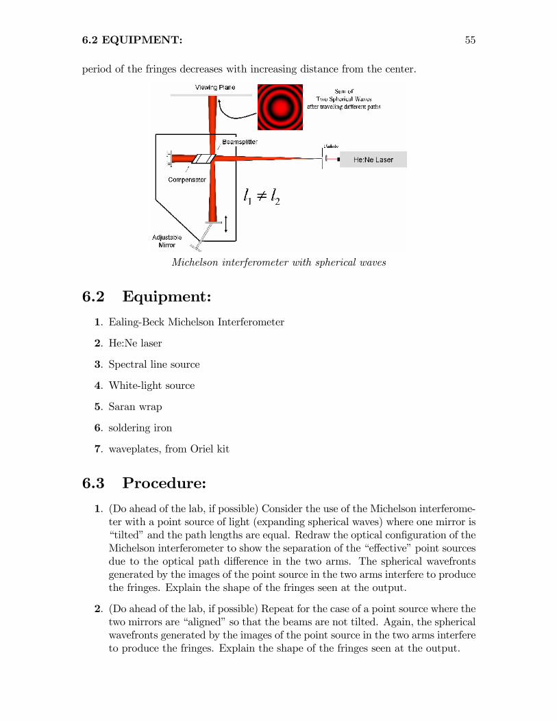
6.2 EQUIPMENT: 55
period of the fringes decreases with increasing distance from the center.
Michelson interferometer with spherical waves
6.2 Equipment:
1. Ealing-Beck Michelson Interferometer
2. He:Ne laser
3. Spectral line source
4. White-light source
5. Saran wrap
6. soldering iron
7. waveplates, from Oriel kit
6.3 Procedure:
1. (Do ahead of the lab, if possible) Consider the use of the Michelson interferome-ter with a point source of light (expanding spherical waves) where one mirror is�tilted�and the path lengths are equal. Redraw the optical con�guration of theMichelson interferometer to show the separation of the �e¤ective�point sourcesdue to the optical path di¤erence in the two arms. The spherical wavefrontsgenerated by the images of the point source in the two arms interfere to producethe fringes. Explain the shape of the fringes seen at the output.
2. (Do ahead of the lab, if possible) Repeat for the case of a point source where thetwo mirrors are �aligned�so that the beams are not tilted. Again, the sphericalwavefronts generated by the images of the point source in the two arms interfereto produce the fringes. Explain the shape of the fringes seen at the output.
56CHAPTER 6 LAB#5: DIVISION-OF-AMPLITUDE INTERFERENCE
3. In the �rst part of the lab, use a lens to expand the laser beam into a sphericalwave. The mirrors generate images of the source of the spherical wave, and theresulting spherical wavefronts superpose. The squared magnitude of the spatialmodulation of the superposition is the visible fringe pattern. The drawingsbelow give an idea of the form of the fringes that will be visible for variouscon�gurations of the two mirrors when used with spherical waves.
4. Once you have obtained circular fringes that are approximately centered, movethe translatable mirror to increase or decrease the optical path di¤erence. (besure that you know which!). Note the direction that the fringes move; in otherwords, do they appear from or disappear into the center? Explain.
5. Note that fringes also are produced at the input end of the interferometer. Howdo they di¤er from those at the output end?
6. Place Polaroid �lters in each path and note the e¤ect on the interference patternas the relative polarizations of the beams are changed. Also try the sameexperiment with �=4 plates, �=2 plates, and the circular polarizer.
7. Place a piece of plastic wrap in one arm of the interferometer. Describe andexplain its e¤ect.
8. Place a spherical lens (best if the focal length f is very long) in the beam at theinput end and note the e¤ect on the fringes. Repeat with the lens in one arm.
9. Put a source of heat in or under one of the arms of the interferometer; yourhand will work (if you are warmblooded!), but a more intense source such as asoldering iron works better. Note the e¤ect.
10. The wavefronts in the second part of the lab should be approximately planar;use a second lens to generate collimated light. See if you can generate a patternthat is all white or all black, in other words, the pattern is a single bright ordark fringe. When you have generated the dark fringe, try the experiment withthe heat source in one arm again.
6.4 Questions:
1. (Already mentioned in the text) Compute the coherence time and coherencelength for white light, which may be modeled as containing �equal amounts�oflight with all frequencies from the blue (�= 400 nm) to the red (� �= 700 nm).
2. (Already mentioned in the text) Redraw the optical con�guration of the Michel-son to show the separation of the e¤ective point sources due to the path-lengthdi¤erence in the two arms of the interferometer.
3. Explain the direction of motion of the circular fringes when the path lengthis changed, i.e., what directions do the circular fringes move if the OPL isincreased? What if OPL is decreased?.
6.5 REFERENCES: 57
4. When the Michelson is used with collimated light, explain how a single darkfringe can be obtained. Where did the light intensity go?
5. Explain what happens when a piece of glass (or other material) is placed in onearm.
6.5 References:
Optics, E. Hecht, sec 9.4

Chapter 7
Lab #6: Di¤raction
We are able to determine locations of images and their magni�cations by using theconcept of light as a �ray�(geometrical optics). However, the concept of light as a�wave�also is fundamental to imaging, particularly in its manifestation in �di¤rac-tion�, which is the fundamental limitation on the action of an optical imaging system.�Interference�and �di¤raction�may be interpreted as the same phenomenon, di¤er-ing only in the number of sources involved (interference =) few sources, say 2 - 10;di¤raction =) many sources, up to an in�nite number). The theory of di¤ractionleads to the theoretical limit to the performance of an imaging system.
7.1 Theory:
This lab will investigate the di¤raction patterns generated from apertures of di¤er-ent shapes and observed at di¤erent distances. As we have mentioned, the physicalprocess that results in observable di¤raction patterns is identical to that responsi-ble for interference. In the latter case, we generally speak of the intensity patternsgenerated by light after passing through a few apertures whose size(s) generally aresmaller than the distance between them. The term di¤raction usually is applied tothe process either for a single large aperture, or (equivalently) a large number of small(usually in�nitesimal) contiguous apertures.In studies of both interference and di¤raction, the patterns are most obvious if
the illumination is coherent, which means that the phase of the sinusoidal electric�elds is rigidly deterministic. In other words, knowledge of the phase of the �eldat some point in space and/or time determines the phase at other points in spaceand/or time. Coherence has two �avors: spatial and temporal. For spatially coherentlight, the phase di¤erence �� � �1��2 of the electric �eld measured at two di¤erentpoints at the same time at two points in space separated by a vector distance �rremains constant for all times and for all such points in space. If the phase di¤erencemeasured at the SAME location at two di¤erent times separated by �t � t1 � t2 isthe same for all points in space, the light is temporally coherent. Light from a lasermay be considered to be BOTH spatially and temporally coherent. The propertiesof coherent light allow phase di¤erences of light that has traveled di¤erent paths to
59
60 CHAPTER 7 LAB #6: DIFFRACTION
be made visible, since the phase di¤erence is constant with time. In interference,the e¤ect often results in a sinusoidal fringe pattern in space. In di¤raction, thephase di¤erence of light from di¤erent points in the same large source can be seenas a similar pattern of dark and bright fringes, though not (usually) with sinusoidalspacing.Observed di¤raction patterns from the same object usually look very di¤erent at
di¤erent distances to the observation plane. If viewed very close to the aperture (inthe Rayleigh-Sommerfeld di¤raction region), then Huygens�principle says that theamplitude of the electric �eld is the summation (integral) of the spherical wavefrontsgenerated by each point in the aperture. The resulting amplitude pattern may bequite complicated to evaluate. If observed somewhat farther from the aperture, thespherical wavefronts may be accurately approximated by paraboloidal wavefronts.The approximation applies in the near �eld, or the Fresnel di¤raction region. Ifviewed at a large distance compared to the extent of the object, the light from di¤erentlocations in the aperture may be accurately modeled as plane waves with di¤erentwavefront tilts. This occurs in the Fraunhofer di¤raction region.
7.1.1 Fresnel Di¤raction
In the Fresnel di¤raction region (where the distance between the object and theobservation plane is small compared to the size of the object). The di¤raction patternresembles the original object with �fuzzy�or �ringing�edges. If the size of the objectis increased, so will be the Fresnel di¤raction pattern. If the distance between theobject and the observation is increased, though still within the Fresnel di¤ractionregion, the size of the �ringing�artifacts increases. In general, the Fresnel di¤ractionpattern of an object f [x; y] observed at a distance z1 �downstream�is proportionalto the expression:
g [x; y] =1
i�0z1exp
�+2�iz1�0
� ZZ +1
�1f [x� �; y � �] exp
��i�(�
2 + �2)
�0z1
�d� d�
=1
i�0z1exp
�+2�iz1�0
��f [x; y] � exp
��i�(x
2 + y2)
�0z1
��= f [x; y] �
�1
i�0z1exp
�+2�iz1�0
�exp
��i�(x
2 + y2)
�0z1
��� f [x; y] � h [x; y; z1]
where h [x; y; z1] is the �impulse response of light propagation� for wavelength �0and axial distance z1. The calculation has the form of the mathematical operationof convolution of the object pattern and a quadratic-phase pattern (which representsthe paraboloidal shape of the individual waves). The convolution operation involves atranslation of the reversed input function in the integration coordinates [�; �], followed
by multiplication by the quadratic-phase factor exph� i�(�2+�2)
�0z1
iand then evaluation
of the area for each value of the output coordinates [x; y]. Thus it is �complicated�and computationally intensive.
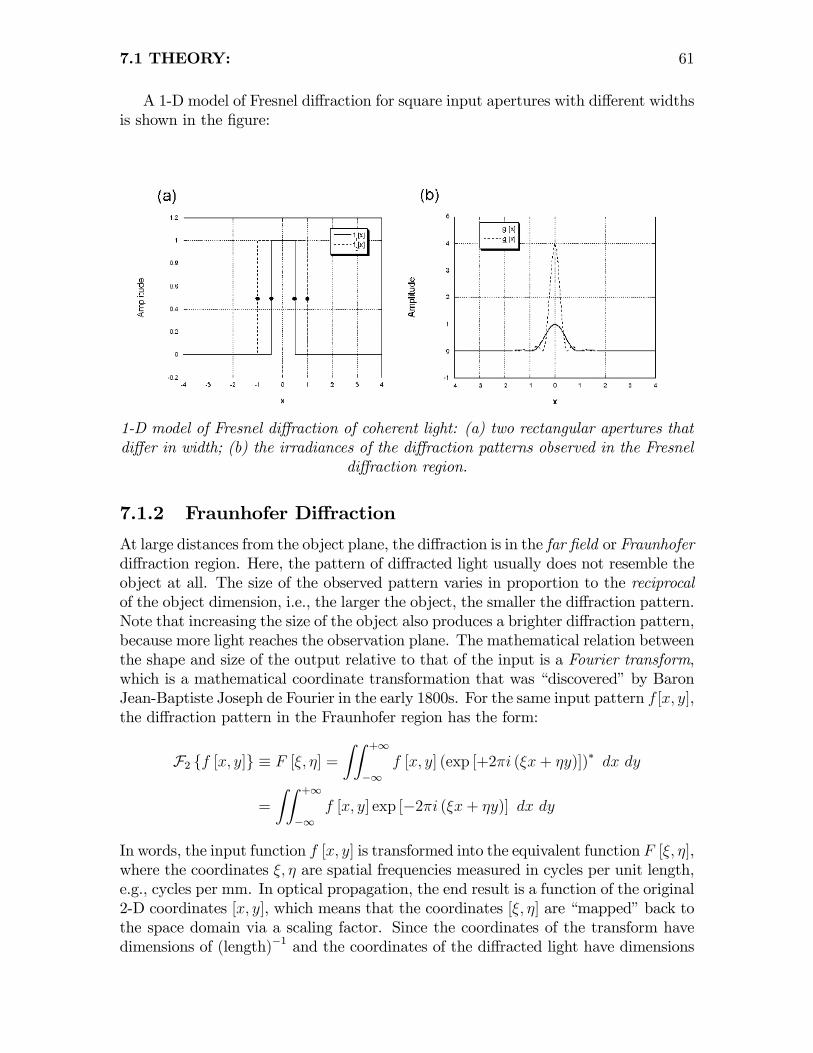
7.1 THEORY: 61
A 1-D model of Fresnel di¤raction for square input apertures with di¤erent widthsis shown in the �gure:
1-D model of Fresnel di¤raction of coherent light: (a) two rectangular apertures thatdi¤er in width; (b) the irradiances of the di¤raction patterns observed in the Fresnel
di¤raction region.
7.1.2 Fraunhofer Di¤raction
At large distances from the object plane, the di¤raction is in the far �eld or Fraunhoferdi¤raction region. Here, the pattern of di¤racted light usually does not resemble theobject at all. The size of the observed pattern varies in proportion to the reciprocalof the object dimension, i.e., the larger the object, the smaller the di¤raction pattern.Note that increasing the size of the object also produces a brighter di¤raction pattern,because more light reaches the observation plane. The mathematical relation betweenthe shape and size of the output relative to that of the input is a Fourier transform,which is a mathematical coordinate transformation that was �discovered�by BaronJean-Baptiste Joseph de Fourier in the early 1800s. For the same input pattern f [x; y],the di¤raction pattern in the Fraunhofer region has the form:
F2 ff [x; y]g � F [�; �] =ZZ +1
�1f [x; y] (exp [+2�i (�x+ �y)])� dx dy
=
ZZ +1
�1f [x; y] exp [�2�i (�x+ �y)] dx dy
In words, the input function f [x; y] is transformed into the equivalent function F [�; �],where the coordinates �; � are spatial frequencies measured in cycles per unit length,e.g., cycles per mm. In optical propagation, the end result is a function of the original2-D coordinates [x; y], which means that the coordinates [�; �] are �mapped�back tothe space domain via a scaling factor. Since the coordinates of the transform havedimensions of (length)�1 and the coordinates of the di¤racted light have dimensions
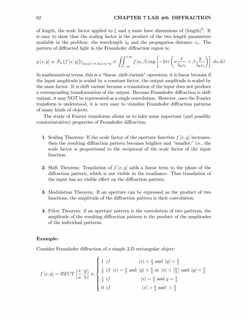
62 CHAPTER 7 LAB #6: DIFFRACTION
of length, the scale factor applied to � and � must have dimensions of (length)2. Itis easy to show that the scaling factor is the product of the two length parametersavailable in the problem: the wavelength �0 and the propagation distance z1. Thepattern of di¤racted light in the Fraunhofer di¤raction region is:
g [x; y] / F2 ff [x; y]gj�0z1�!x;�0z1�!y �ZZ +1
�1f [�; �] exp
��2�i
��x
�0z1+ �
y
�0z1
��d� d�
In mathematical terms, this is a �linear, shift-variant�operation; it is linear because ifthe input amplitude is scaled by a constant factor, the output amplitude is scaled bythe same factor. It is shift variant because a translation of the input does not producea corresponding transformation of the output. Because Fraunhofer di¤raction is shiftvariant, it may NOT be represented as a single convolution. However, once the Fouriertransform is understood, it is very easy to visualize Fraunhofer di¤raction patternsof many kinds of objects.The study of Fourier transforms allows us to infer some important (and possibly
counterintuitive) properties of Fraunhofer di¤raction:
1. Scaling Theorem: If the scale factor of the aperture function f [x; y] increases,then the resulting di¤raction pattern becomes brighter and �smaller,�i.e., thescale factor is proportional to the reciprocal of the scale factor of the inputfunction.
2. Shift Theorem: Translation of f [x; y] adds a linear term to the phase of thedi¤raction pattern, which is not visible in the irradiance. Thus translation ofthe input has no visible e¤ect on the di¤raction pattern.
3. Modulation Theorem: If an aperture can be expressed as the product of twofunctions, the amplitude of the di¤raction pattern is their convolution.
4. Filter Theorem: if an aperture pattern is the convolution of two patterns, theamplitude of the resulting di¤raction pattern is the product of the amplitudesof the individual patterns.
Example:
Consider Fraunhofer di¤raction of a simple 2-D rectangular object:
f [x; y] = RECThxa;y
b
i�
8>>>>>><>>>>>>:
1 if jxj < a2and jyj < b
2
12if jxj = a
2and jyj < b
2or jxj <
�� b2
�� and jyj = b2
14if jxj = a
2and y = b
2
0 if jxj > a2and > b
2
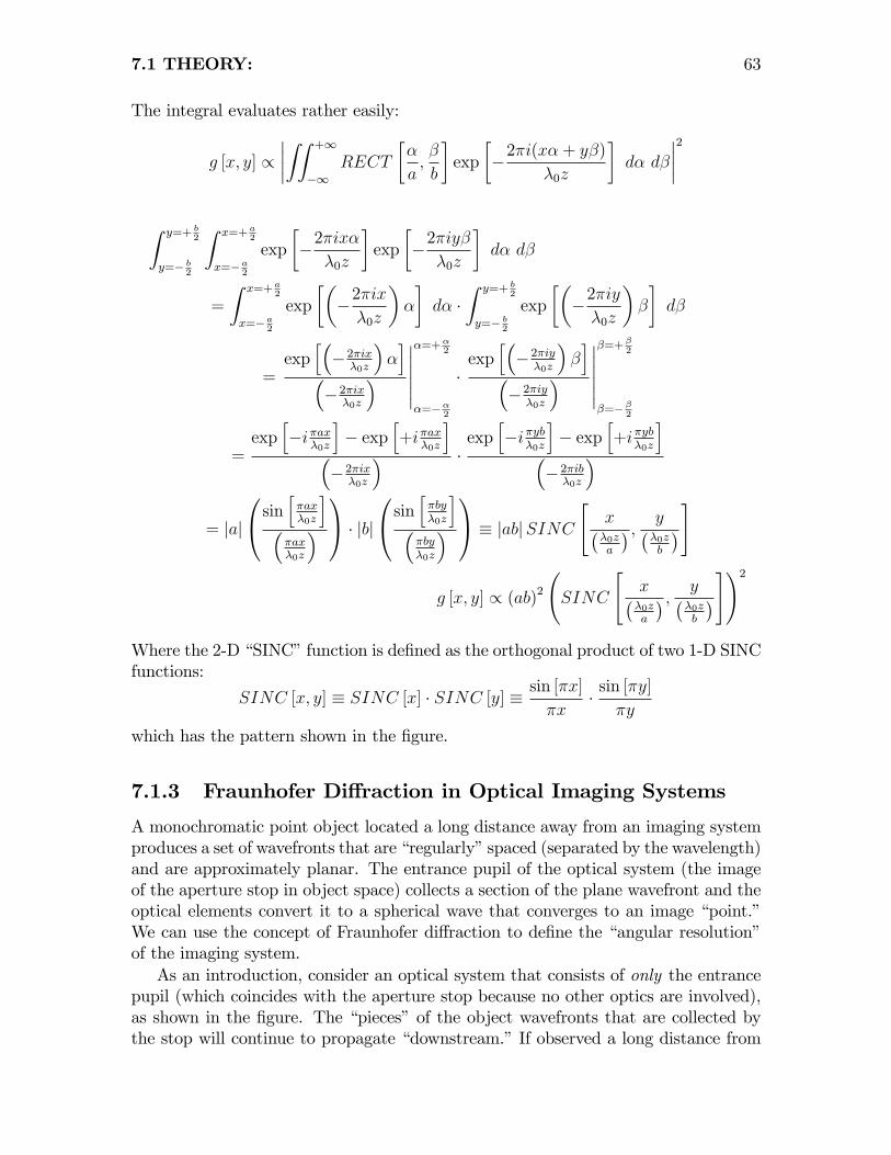
7.1 THEORY: 63
The integral evaluates rather easily:
g [x; y] /����ZZ +1
�1RECT
��
a;�
b
�exp
��2�i(x� + y�)
�0z
�d� d�
����2
Z y=+ b2
y=� b2
Z x=+a2
x=�a2
exp
��2�ix��0z
�exp
��2�iy��0z
�d� d�
=
Z x=+a2
x=�a2
exp
���2�ix�0z
��
�d� �
Z y=+ b2
y=� b2
exp
���2�iy�0z
��
�d�
=exp
h��2�ix
�0z
��i
��2�ix
�0z
��������=+�
2
�=��2
�exp
h��2�iy
�0z
��i
��2�iy
�0z
��������=+�
2
�=��2
=exp
h�i�ax
�0z
i� exp
h+i�ax
�0z
i��2�ix
�0z
� �exp
h�i�yb
�0z
i� exp
h+i�yb
�0z
i��2�ib�0z
�= jaj
0@sinh�ax�0z
i��ax�0z
�1A � jbj
0@sinh�by�0z
i��by�0z
�1A � jabjSINC
"x��0za
� ; y��0zb
�#
g [x; y] / (ab)2 SINC
"x��0za
� ; y��0zb
�#!2Where the 2-D �SINC�function is de�ned as the orthogonal product of two 1-D SINCfunctions:
SINC [x; y] � SINC [x] � SINC [y] � sin [�x]
�x� sin [�y]
�y
which has the pattern shown in the �gure.
7.1.3 Fraunhofer Di¤raction in Optical Imaging Systems
A monochromatic point object located a long distance away from an imaging systemproduces a set of wavefronts that are �regularly�spaced (separated by the wavelength)and are approximately planar. The entrance pupil of the optical system (the imageof the aperture stop in object space) collects a section of the plane wavefront and theoptical elements convert it to a spherical wave that converges to an image �point.�We can use the concept of Fraunhofer di¤raction to de�ne the �angular resolution�of the imaging system.As an introduction, consider an optical system that consists of only the entrance
pupil (which coincides with the aperture stop because no other optics are involved),as shown in the �gure. The �pieces�of the object wavefronts that are collected bythe stop will continue to propagate �downstream.�If observed a long distance from
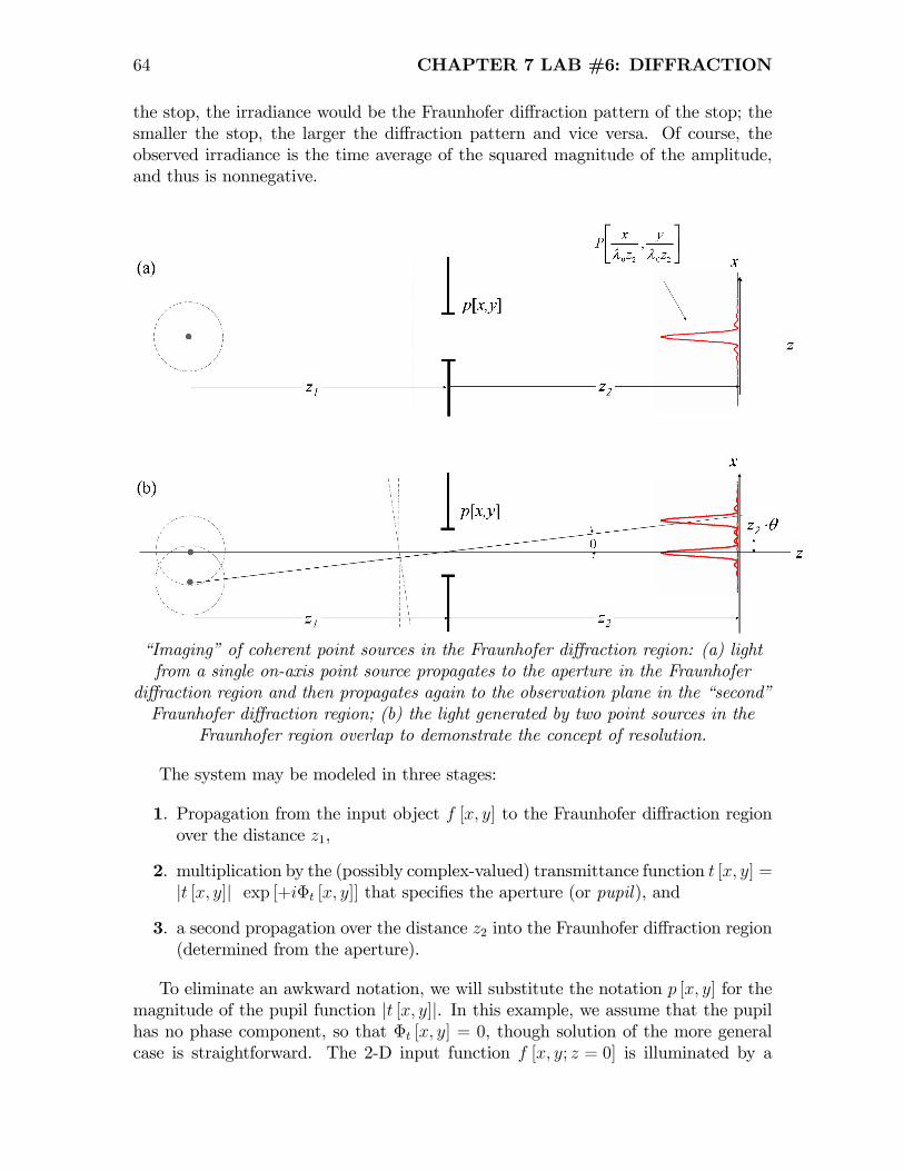
64 CHAPTER 7 LAB #6: DIFFRACTION
the stop, the irradiance would be the Fraunhofer di¤raction pattern of the stop; thesmaller the stop, the larger the di¤raction pattern and vice versa. Of course, theobserved irradiance is the time average of the squared magnitude of the amplitude,and thus is nonnegative.
�Imaging�of coherent point sources in the Fraunhofer di¤raction region: (a) lightfrom a single on-axis point source propagates to the aperture in the Fraunhofer
di¤raction region and then propagates again to the observation plane in the �second�Fraunhofer di¤raction region; (b) the light generated by two point sources in the
Fraunhofer region overlap to demonstrate the concept of resolution.
The system may be modeled in three stages:
1. Propagation from the input object f [x; y] to the Fraunhofer di¤raction regionover the distance z1,
2. multiplication by the (possibly complex-valued) transmittance function t [x; y] =jt [x; y]j exp [+i�t [x; y]] that speci�es the aperture (or pupil), and
3. a second propagation over the distance z2 into the Fraunhofer di¤raction region(determined from the aperture).
To eliminate an awkward notation, we will substitute the notation p [x; y] for themagnitude of the pupil function jt [x; y]j. In this example, we assume that the pupilhas no phase component, so that �t [x; y] = 0, though solution of the more generalcase is straightforward. The 2-D input function f [x; y; z = 0] is illuminated by a
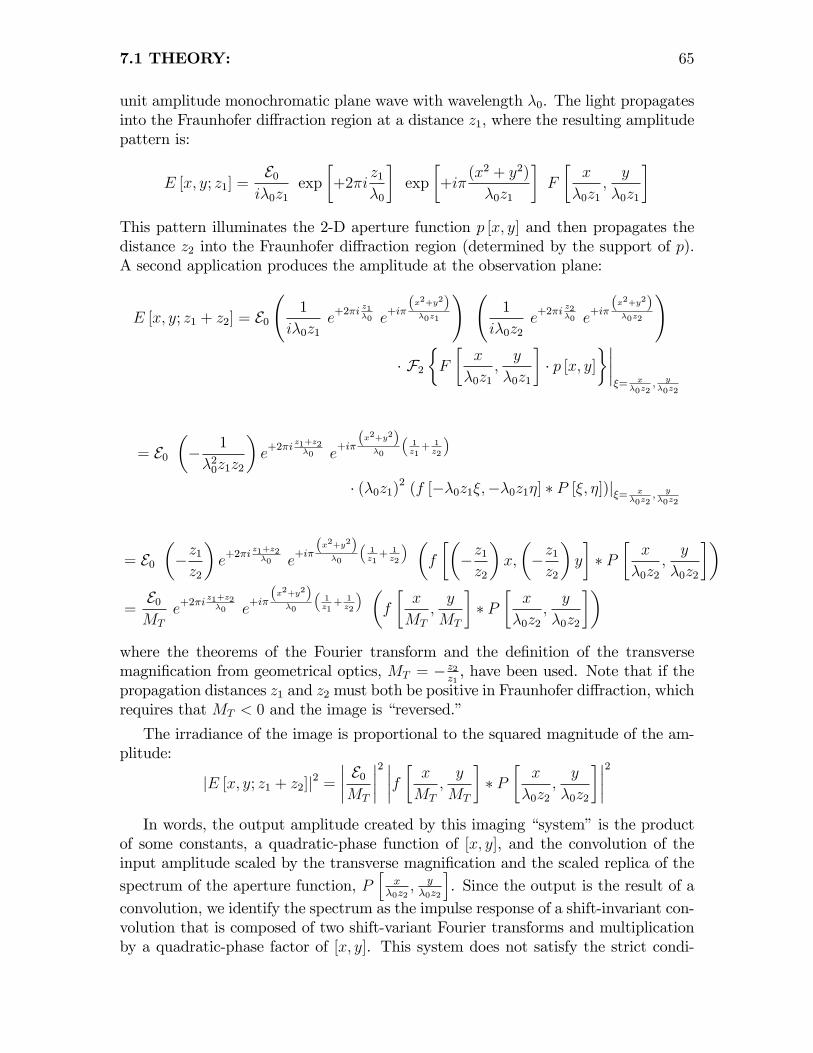
7.1 THEORY: 65
unit amplitude monochromatic plane wave with wavelength �0. The light propagatesinto the Fraunhofer di¤raction region at a distance z1, where the resulting amplitudepattern is:
E [x; y; z1] =E0i�0z1
exp
�+2�i
z1�0
�exp
�+i�
(x2 + y2)
�0z1
�F
�x
�0z1;y
�0z1
�This pattern illuminates the 2-D aperture function p [x; y] and then propagates thedistance z2 into the Fraunhofer di¤raction region (determined by the support of p).A second application produces the amplitude at the observation plane:
E [x; y; z1 + z2] = E0
1
i�0z1e+2�i
z1�0 e
+i�(x2+y2)�0z1
! 1
i�0z2e+2�i
z2�0 e
+i�(x2+y2)�0z2
!
� F2�F
�x
�0z1;y
�0z1
�� p [x; y]
������= x
�0z2; y�0z2
= E0�� 1
�20z1z2
�e+2�i
z1+z2�0 e
+i�(x2+y2)
�0
�1z1+ 1z2
�
� (�0z1)2 (f [��0z1�;��0z1�] � P [�; �])j�= x�0z2
; y�0z2
= E0��z1z2
�e+2�i
z1+z2�0 e
+i�(x2+y2)
�0
�1z1+ 1z2
� �f
���z1z2
�x;
��z1z2
�y
�� P
�x
�0z2;y
�0z2
��=E0MT
e+2�i
z1+z2�0 e
+i�(x2+y2)
�0
�1z1+ 1z2
� �f
�x
MT
;y
MT
�� P
�x
�0z2;y
�0z2
��where the theorems of the Fourier transform and the de�nition of the transversemagni�cation from geometrical optics, MT = � z2
z1, have been used. Note that if the
propagation distances z1 and z2 must both be positive in Fraunhofer di¤raction, whichrequires that MT < 0 and the image is �reversed.�
The irradiance of the image is proportional to the squared magnitude of the am-plitude:
jE [x; y; z1 + z2]j2 =���� E0MT
����2 ����f � xMT
;y
MT
�� P
�x
�0z2;y
�0z2
�����2In words, the output amplitude created by this imaging �system�is the product
of some constants, a quadratic-phase function of [x; y], and the convolution of theinput amplitude scaled by the transverse magni�cation and the scaled replica of thespectrum of the aperture function, P
hx
�0z2; y�0z2
i. Since the output is the result of a
convolution, we identify the spectrum as the impulse response of a shift-invariant con-volution that is composed of two shift-variant Fourier transforms and multiplicationby a quadratic-phase factor of [x; y]. This system does not satisfy the strict condi-
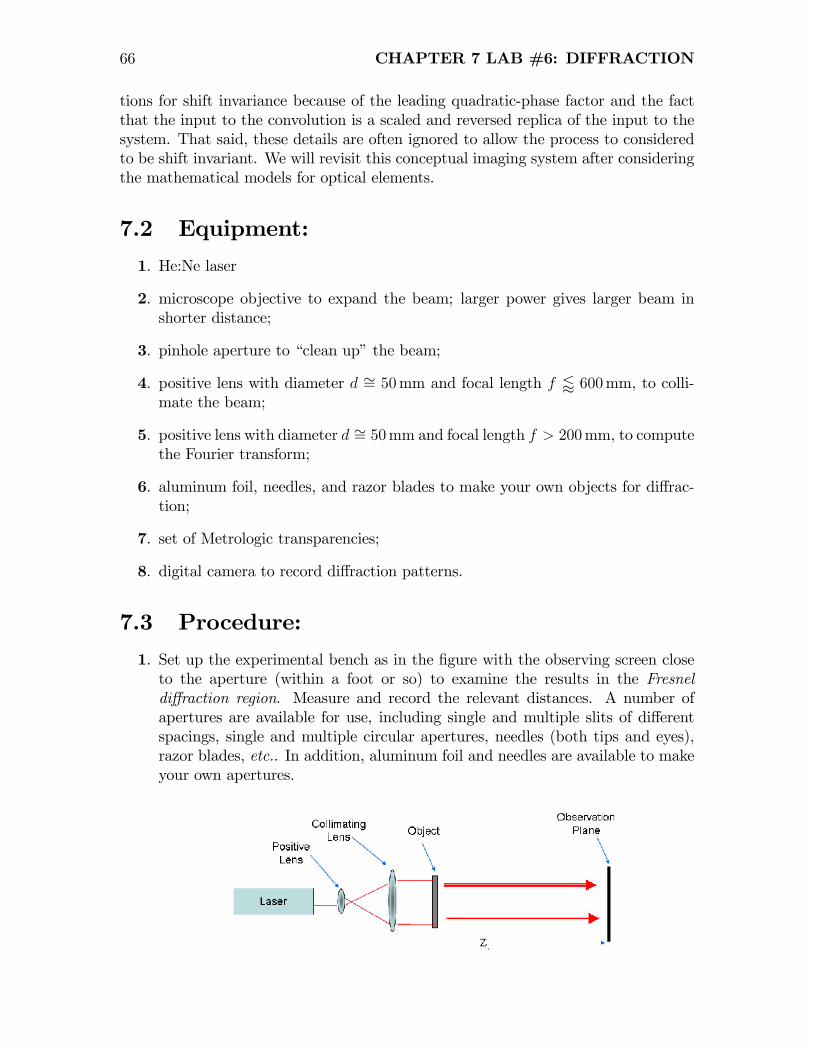
66 CHAPTER 7 LAB #6: DIFFRACTION
tions for shift invariance because of the leading quadratic-phase factor and the factthat the input to the convolution is a scaled and reversed replica of the input to thesystem. That said, these details are often ignored to allow the process to consideredto be shift invariant. We will revisit this conceptual imaging system after consideringthe mathematical models for optical elements.
7.2 Equipment:
1. He:Ne laser
2. microscope objective to expand the beam; larger power gives larger beam inshorter distance;
3. pinhole aperture to �clean up�the beam;
4. positive lens with diameter d �= 50mm and focal length f / 600mm, to colli-mate the beam;
5. positive lens with diameter d �= 50mm and focal length f > 200mm, to computethe Fourier transform;
6. aluminum foil, needles, and razor blades to make your own objects for di¤rac-tion;
7. set of Metrologic transparencies;
8. digital camera to record di¤raction patterns.
7.3 Procedure:
1. Set up the experimental bench as in the �gure with the observing screen closeto the aperture (within a foot or so) to examine the results in the Fresneldi¤raction region. Measure and record the relevant distances. A number ofapertures are available for use, including single and multiple slits of di¤erentspacings, single and multiple circular apertures, needles (both tips and eyes),razor blades, etc.. In addition, aluminum foil and needles are available to makeyour own apertures.
7.3 PROCEDURE: 67
Apparatus for viewing Fresnel di¤raction patterns (and Fraunhofer patterns ifz1 is su¢ ciently large).
(a) Begin with a single slit, a square aperture, or a circular aperture. Note theform of the di¤raction pattern. For example, sketch how its �brightness�changes with position and note the sizes and locations of any features. Fora slit or circular aperture, you should note light and dark regions in thepattern; measure the positions of some maxima and minima (at least 5).Use the data to derive a scale of the pattern. Sketch the pattern notingthe scale.
(b) Repeat the previous step with a �wider�slit or aperture. Note the di¤er-ence in the results.
(c) Vary the distance between the screen and the di¤racting object. Repeatmeasurements. What is the relation between the change in distance andthe change in scale of the pattern? Repeat for 5 di¤erent distances wherethe character of the pattern remains the same.
(d) Repeat the procedure with a knife edge as the object. Sketch the patternobserved. You will see that the intensity distribution near the edge ofthe geometric shadow is not a sharp transition, but rather an undulatorypattern; a magnifying lens, microscope, or digital camera may be helpful toview the pattern, but BE SURE THAT THE LASER LIGHT HAS BEENATTENUATED SUFFICIENTLY.
2. Now observe the di¤raction pattern far from the aperture (several feet awayfor a small aperture, a proportionally larger distance for a larger aperture) toexamine Fraunhofer di¤raction. You may �fold� the pattern with one or twomirrors or you may use a lens to �image�the pattern, i.e., to bring the image ofthe pattern created �a long distance away�much closer to the object. Whichevermethod you use, be sure to use the same setup for all measurements.
(a) For an aperture of a known �xed (small) size, increase the distance tothe observation plane as much as you can. Estimate the location of thetransition between the Fresnel and Fraunhofer di¤raction regions (this willcertainly be ill-de�ned and �fuzzy�). Record and justify your measure-ment.
(b) Add another lens to the system as shown below to �bring in�nity closer�
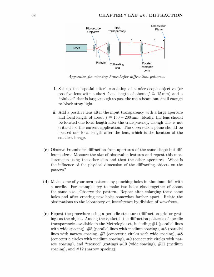
68 CHAPTER 7 LAB #6: DIFFRACTION
Apparatus for viewing Fraunhofer di¤raction patterns.
i. Set up the �spatial �lter� consisting of a microscope objective (orpositive lens with a short focal length of about f �= 15mm) and a�pinhole�that is large enough to pass the main beam but small enoughto block stray light.
ii. Add a positive lens after the input transparency with a large apertureand focal length of about f �= 150� 200mm. Ideally, the lens shouldbe located one focal length after the transparency, though this is notcritical for the current application. The observation plane should belocated one focal length after the lens, which is the location of thesmallest image.
(c) Observe Fraunhofer di¤raction from apertures of the same shape but dif-ferent sizes. Measure the size of observable features and repeat this mea-surements using the other slits and then the other apertures. What isthe in�uence of the physical dimension of the di¤racting objects on thepattern?
(d) Make some of your own patterns by punching holes in aluminum foil witha needle. For example, try to make two holes close together of aboutthe same size. Observe the pattern. Repeat after enlarging these sameholes and after creating new holes somewhat farther apart. Relate theobservations to the laboratory on interference by division of wavefront.
(e) Repeat the procedure using a periodic structure (di¤raction grid or grat-ing) as the object. Among these, sketch the di¤raction patterns of speci�ctransparencies available in the Metrologic set, including #4 (parallel lineswith wide spacing), #5 (parallel lines with medium spacing), #6 (parallellines with narrow spacing, #7 (concentric circles with wide spacing), #8(concentric circles with medium spacing), #9 (concentric circles with nar-row spacing), and �crossed�gratings #10 (wide spacing), #11 (mediumspacing), and #12 (narrow spacing).
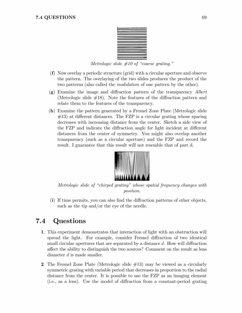
7.4 QUESTIONS 69
Metrologic slide #10 of �coarse grating.�
(f) Now overlay a periodic structure (grid) with a circular aperture and observethe pattern. The overlaying of the two slides produces the product of thetwo patterns (also called the modulation of one pattern by the other).
(g) Examine the image and di¤raction pattern of the transparency Albert(Metrologic slide #18). Note the features of the di¤raction pattern andrelate them to the features of the transparency.
(h) Examine the pattern generated by a Fresnel Zone Plate (Metrologic slide#13) at di¤erent distances. The FZP is a circular grating whose spacingdecreases with increasing distance from the center. Sketch a side view ofthe FZP and indicate the di¤raction angle for light incident at di¤erentdistances from the center of symmetry. You might also overlap anothertransparency (such as a circular aperture) and the FZP and record theresult. I guarantee that this result will not resemble that of part d.
Metrologic slide of �chirped grating�whose spatial frequency changes withposition.
(i) If time permits, you can also �nd the di¤raction patterns of other objects,such as the tip and/or the eye of the needle.
7.4 Questions
1. This experiment demonstrates that interaction of light with an obstruction willspread the light. For example, consider Fresnel di¤raction of two identicalsmall circular apertures that are separated by a distance d. How will di¤ractiona¤ect the ability to distinguish the two sources? Comment on the result as lensdiameter d is made smaller.
2. The Fresnel Zone Plate (Metrologic slide #13) may be viewed as a circularlysymmetric grating with variable period that decreases in proportion to the radialdistance from the center. It is possible to use the FZP as an imaging element(i.e., as a lens). Use the model of di¤raction from a constant-period grating
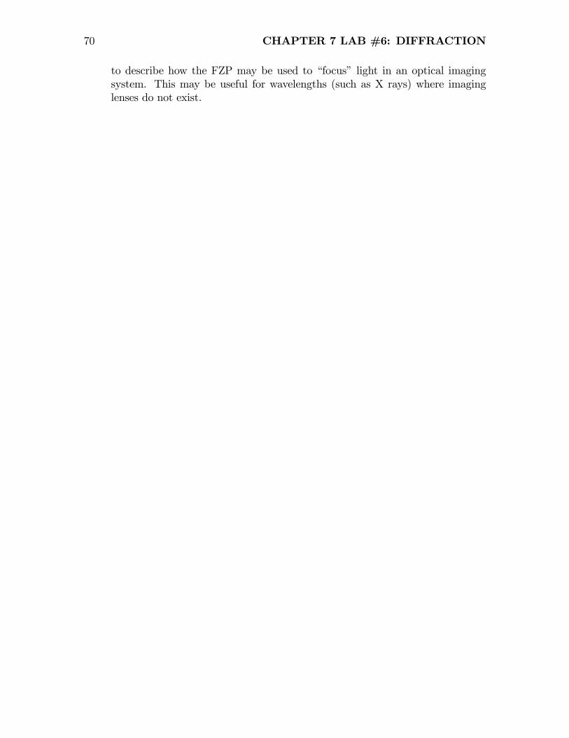
70 CHAPTER 7 LAB #6: DIFFRACTION
to describe how the FZP may be used to �focus� light in an optical imagingsystem. This may be useful for wavelengths (such as X rays) where imaginglenses do not exist.
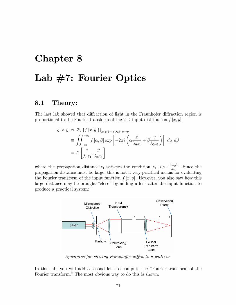
Chapter 8
Lab #7: Fourier Optics
8.1 Theory:
The last lab showed that di¤raction of light in the Fraunhofer di¤raction region isproportional to the Fourier transform of the 2-D input distribution.f [x; y]:
g [x; y] / F2 ff [x; y]gj�0z1�!x;�0z1�!y
�ZZ +1
�1f [�; �] exp
��2�i
��x
�0z1+ �
y
�0z1
��d� d�
= F
�x
�0z1;y
�0z1
�where the propagation distance z1 satis�es the condition z1 >>
x2+y2
�0. Since the
propagation distance must be large, this is not a very practical means for evaluatingthe Fourier transform of the input function f [x; y]. However, you also saw how thislarge distance may be brought �close�by adding a lens after the input function toproduce a practical system:
Apparatus for viewing Fraunhofer di¤raction patterns.
In this lab, you will add a second lens to compute the �Fourier transform of theFourier transform.�The most obvious way to do this is shown:
71
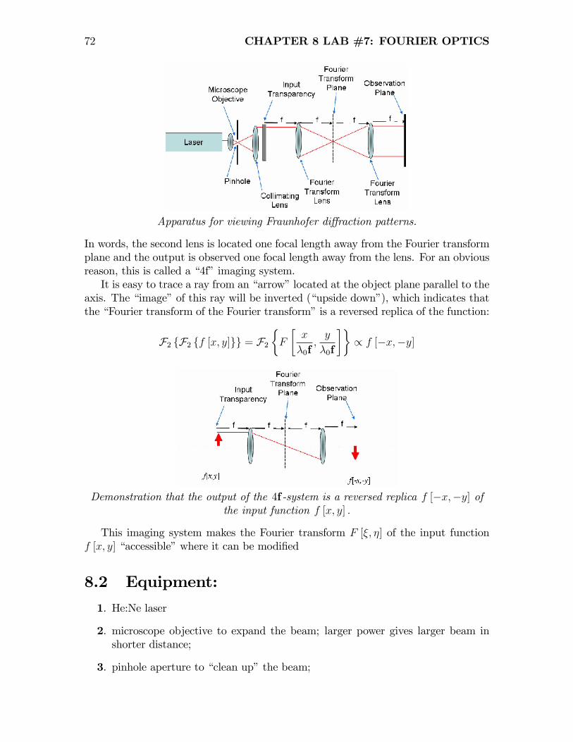
72 CHAPTER 8 LAB #7: FOURIER OPTICS
Apparatus for viewing Fraunhofer di¤raction patterns.
In words, the second lens is located one focal length away from the Fourier transformplane and the output is observed one focal length away from the lens. For an obviousreason, this is called a �4f�imaging system.It is easy to trace a ray from an �arrow�located at the object plane parallel to the
axis. The �image�of this ray will be inverted (�upside down�), which indicates thatthe �Fourier transform of the Fourier transform�is a reversed replica of the function:
F2 fF2 ff [x; y]gg = F2�F
�x
�0f;y
�0f
��/ f [�x;�y]
Demonstration that the output of the 4f-system is a reversed replica f [�x;�y] ofthe input function f [x; y] :
This imaging system makes the Fourier transform F [�; �] of the input functionf [x; y] �accessible�where it can be modi�ed
8.2 Equipment:
1. He:Ne laser
2. microscope objective to expand the beam; larger power gives larger beam inshorter distance;
3. pinhole aperture to �clean up�the beam;
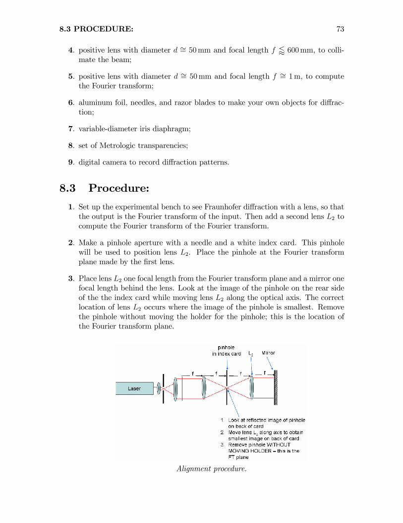
8.3 PROCEDURE: 73
4. positive lens with diameter d �= 50mm and focal length f / 600mm, to colli-mate the beam;
5. positive lens with diameter d �= 50mm and focal length f �= 1m, to computethe Fourier transform;
6. aluminum foil, needles, and razor blades to make your own objects for di¤rac-tion;
7. variable-diameter iris diaphragm;
8. set of Metrologic transparencies;
9. digital camera to record di¤raction patterns.
8.3 Procedure:
1. Set up the experimental bench to see Fraunhofer di¤raction with a lens, so thatthe output is the Fourier transform of the input. Then add a second lens L2 tocompute the Fourier transform of the Fourier transform.
2. Make a pinhole aperture with a needle and a white index card. This pinholewill be used to position lens L2. Place the pinhole at the Fourier transformplane made by the �rst lens.
3. Place lens L2 one focal length from the Fourier transform plane and a mirror onefocal length behind the lens. Look at the image of the pinhole on the rear sideof the the index card while moving lens L2 along the optical axis. The correctlocation of lens L2 occurs where the image of the pinhole is smallest. Removethe pinhole without moving the holder for the pinhole; this is the location ofthe Fourier transform plane.
Alignment procedure.
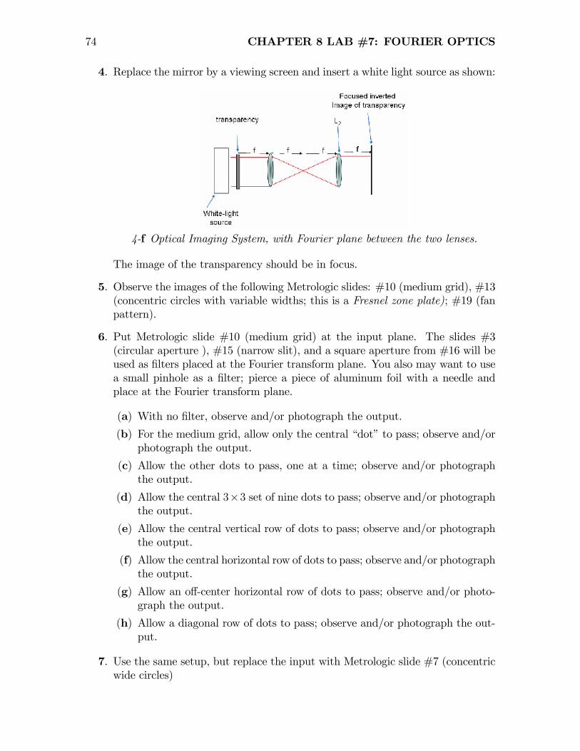
74 CHAPTER 8 LAB #7: FOURIER OPTICS
4. Replace the mirror by a viewing screen and insert a white light source as shown:
4-f Optical Imaging System, with Fourier plane between the two lenses.
The image of the transparency should be in focus.
5. Observe the images of the following Metrologic slides: #10 (medium grid), #13(concentric circles with variable widths; this is a Fresnel zone plate); #19 (fanpattern).
6. Put Metrologic slide #10 (medium grid) at the input plane. The slides #3(circular aperture ), #15 (narrow slit), and a square aperture from #16 will beused as �lters placed at the Fourier transform plane. You also may want to usea small pinhole as a �lter; pierce a piece of aluminum foil with a needle andplace at the Fourier transform plane.
(a) With no �lter, observe and/or photograph the output.
(b) For the medium grid, allow only the central �dot�to pass; observe and/orphotograph the output.
(c) Allow the other dots to pass, one at a time; observe and/or photographthe output.
(d) Allow the central 3�3 set of nine dots to pass; observe and/or photographthe output.
(e) Allow the central vertical row of dots to pass; observe and/or photographthe output.
(f) Allow the central horizontal row of dots to pass; observe and/or photographthe output.
(g) Allow an o¤-center horizontal row of dots to pass; observe and/or photo-graph the output.
(h) Allow a diagonal row of dots to pass; observe and/or photograph the out-put.
7. Use the same setup, but replace the input with Metrologic slide #7 (concentricwide circles)
8.4 REFERENCES: 75
(a) With no �lter, observe and/or photograph the output.
(b) Use the horizontal slit (slide #15) to allow part of the di¤racted light topass; observe and/or photograph the output.
8. Use slide #22 (simulation of cloud-chamber photograph) as the object and slide#26 (transparent bar with obstruction at center) as the �lter. Position the �lterso that the transparent bar is perpendicular to the lines in the input.
9. Use slide #25 as the input and #26 as the �lter.
(a) Orient the �lter bar in the vertical direction; observe the output.
(b) Orient the �lter bar in the horizontal direction; observe the output
10. Use slide #26 (halftone image of Albert Einstein) as the input and a variable-diameter iris or slides #17 and #18 (circular apertures) as the �lter. Experimentwith the �lter.
8.4 References:
Optics, E. Hecht, Chapter 10, 11

Chapter 9
Lab #8: Computer-GeneratedHolography
9.1 Theory:
In this lab, you will create �holographic�images of synthetic objects. These �computer-generated holograms�(or CGHs) are mappings of the complex amplitude (magnitudeAND phase) of light re�ected from or transmitted by synthetic objects. The wave-fronts that would emerge from the objects are �reconstructed�by the propagationof light through the hologram. Holography is based on the �di¤raction�of light byan object, which may be viewed as a result of Huygens�principle that light propa-gates by creating spherical �wavelets�. A hologram is the record of the interferencepattern generated by the wavefront from an object and from a known source (the ref-erence). Holography was �rst described by Gabor in the 1940s, but did not becomepractical until lasers that produced (nearly) monochromatic light became available inthe 1960s. The modi�cations to the holographic process that were �rst implementedby Leith and Upatnieks vastly improved the process and allowed 3-D objects to bereconstructed.The description of a hologram is based on optical di¤raction, which is in three
regions at increasing distance from the source (or object). The three classes of dif-fraction region are:
1. Rayleigh-Sommerfeld di¤raction, where the light is considered to propagateexactly via spherical waves. The evaluated result is valid at any distance fromthe source.
2. Fresnel di¤raction, where the light is modeled as a parabolic wave (i.e., aquadratic-phase term), valid at a larger distance from the source. In this case,the propagation of light from a 2-D source function f [x; y] over the distance z1is the convolution with the parabolic impulse response h [x; y]
h [x; y] =exp
�+2�i z1
�
�i�z1
exp
�+i�
x2 + y2
�z1
�
77
78CHAPTER 9 LAB #8: COMPUTER-GENERATED HOLOGRAPHY
3. Fraunhofer di¤raction, where di¤racted light is modeled as a plane wave, validat very large distances from the object or source. In this case, the di¤ractionpattern g [x; y] produced by the 2-D input f [x; y] is the 2-D Fourier transformwith appropriately scaled coordinates
g [x; y] / F�x
�z1;y
�z1
�, where F2 ff [x; y]g = F [�; �]
This experiment will consider holography in the Fraunhofer di¤raction region only.We �rst consider the mathematical description of a simple hologram created by twopoint sources in the Fraunhofer di¤raction region. It then concludes with a processfor calculating the pattern for a simple hologram that you will create, print, andreconstruct. In your report of the experiment, you should also model the steps in theholographic process described in the next section.
9.2 Fraunhofer Hologram of Two Point Sources:
The mathematical description of the holographic process evaluated in the Fraunhoferdi¤raction region is straightforward because of the Fourier transform relationshipbetween the input source function and the di¤racted amplitude. Consider the simplecase of two point sources that emit the same monochromatic wavelength � and thatare located in the plane z = 0. For convenience, one source is located �on axis�(at x = y = 0) with unit amplitude, while the relative amplitude of the second (�o¤-axis�) source is a e+i�0, where a is a real number that measures the relative magnitudeand �0 is the relative phase. For convenience in the discussion, we choose a to lie inthe interval 0 � a � 1 so that the o¤-axis source is �fainter�than the on-axis source,though this constraint is not essential. Note that if the relative phase �0 = 0, the twosources are �in phase�, if �0 = ��, then the two sources are �out of phase�, and if�0 = ��
2, the sources are �in quadrature�. The 3-D mathematical expression for the
source function is:
f [x; y; z] = � [x; y; z] + a e+i�0 � [x� x0; y; z] e+i�0
=�� [x; y] + a e+i�0 � [x� x0; y]
�� [z]
The radiation from these sources is observed at the plane de�ned by z = z1, whichis assumed to be su¢ ciently distant so that the spherical waves are suitably approx-imated by plane waves. In other words, the description of Fraunhofer di¤raction isappropriate. In such a case, the observed amplitude s [x; y; z = z1] is proportional tothe Fourier transform of the source function evaluated at suitably scaled coordinates:
s [x; y; z1] / F2 ff [x; y; z]gj�= x�z1
;�= y�z1
=
�1 + a e+i�0 e
�2�i�x0�z1
�x
�1
�x
�z1;y
�z1
�
9.2 FRAUNHOFER HOLOGRAM OF TWO POINT SOURCES: 79
The measurable quantity at the observation plane is the irradiance js [x; y; z1]j2, whichis proportional to:
js [x; y; z1]j2 /�1 + a e+i�0 e
�2�i�x0�z1
�x
��1 + a e�i�0 e
+2�i�x0�z1
�x
�=�1 + a2
�+ 2a cos
�2�
�x0�z1
�x� �0
�=�1 + a2
��1 +
2a
1 + a2cos
�2�
�x0�z1
�x� �0
����1 + a2
��1 +
2a
1 + a2cos [2��0x� �0]
�where �0 � x0
�z1is the spatial frequency of the sinusoidal irradiance pattern observed
at the plane z = z1. This sinusoidal �grating�oscillates over the range of amplitudes(1 + a2)� 2a, and therefore its modulation is:
m ��js [x; y; z1]j2
�max
��js [x; y; z1]j2
�min�
js [x; y; z1]j2�max
+�js [x; y; z1]j2
�min
=[(1 + a2) + 2a]� [(1 + a2)� 2a][(1 + a2) + 2a] + [(1 + a2)� 2a] =
2a
1 + a2
The irradiance at the observation plane may be concisely expressed as:
js [x; y; z1]j2 /1
2(1 +m cos [2��0x� �0])
The modulation is unity if the sources have equal amplitude (a = 1) and approachesm ' 2a if the amplitude of the second source a! 0.The sinusoidal grating generated by light from the two sources conveys evidence
of their mutual existence. The various measurable parameters of the grating (orien-tation, period, phase at the origin, and modulation) are determined by the physicalproperties of the point sources (orientation, separation, relative phase, and relativeamplitude). A recording of the irradiance pattern (as on a photographic emulsion)preserves the evidence of these properties, but it would be desirable to �nd a methodfor �reconstructing� images of the sources from this recording. In other words, wewould like to �nd an �inverse �lter�for the process of generating the sinusoidal grat-ing.To �nd the �inverse �lter� for the process, it is necessary to model the photo-
graphic process mathematically, including the photographic storage of the pattern.We all know that photographic emulsions record �negative�images of the irradiancedistribution, which is more accurately called the scaled �complement�in this context,as the measurable parameter is the optical �transmittance�t, which is in the interval0 � t � 1 and thus is nonnegative. The recorded transmittance t is small where theirradiance js [x; y; z1]j2 is large. If the recording is �linear�, then the transmittance isdoubled if the irradiance is halved. We also assume that the emulsion is �thin�and
80CHAPTER 9 LAB #8: COMPUTER-GENERATED HOLOGRAPHY
records only the interference pattern produced in the plane of the emulsion. �Thick�holograms record interference patterns in three dimensions and their description re-quires further details.
Our goal is to process the emulsion to produce a �hologram�whose optical trans-mittance is a faithful rendition of the complement of the sinusoidal irradiance, in-cluding the period, orientation, initial phase, and modulation. In our simple model,we will assume that the hologram is processed so that exposure to the �average�irradiance (i.e., the �bias� of the grating) produces a transmittance t [x; y; z1] = 1
2,
while the modulation of the transmittance t [x; y; z1] is identical to that of the origi-nal irradiance js [x; y; z1]j2. The appropriate mapping function u
�js [x; y; z1]j2
�is the
complement of the incident irradiance after scaling to half-unit bias:
t [x; y; z1] = u�js [x; y; z1]j2
�=�jsj2�max
� js [x; y; z1]j2
=1
2
�1�m cos
�2�
�x0�z1
�x� �0
��1 [y]
=) 1
2(1� cos [2��0x� �0]) 1 [y] for a = 1
=) 1
2� a cos [2��0x� �0] 1 [y] for a ' 0
where �0 � x0�z1
This recorded pattern t [x; y; z1] is the hologram. In this case, it is asimple sinusoidal pattern along the x-axis and constant along y. Note also how simplethis pattern was to calculate �this is the basis for the idea of computer-generatedholography.
A side comment about �reality� is essential here. In real life, it is no simpletask to develop the emulsion so that the transmittance is proportional to the scaledcomplement of the irradiance. Nonlinear deviations from this ideal behavior thatcomplicate the analysis can easily �creep into� the processing. We will considerthe qualitative e¤ects of the nonlinearities after analyzing the ideal result. Also,this example assumes that the holographic recording is in�nitely large. Though thisassumption seems to be unrealistic, it is no more so than the assumption of Fraunhoferdi¤raction itself, which is only valid within some region near the optical axis.
Now, replace the processed hologram in its original position and reilluminate it bylight from the on-axis source. The illumination is a plane wave that travels down thez-axis. The action of the hologram is to modulate the source illumination to producean amplitude pattern proportional to t [x; y; z1]. The hologram is �reconstructed�by propagating this amplitude distribution to an observation plane �downstream�from the hologram. Consider that the propagation distance to the observation planeis z2, so that the amplitude is observed at the plane de�ned by z = z1 + z2. Ifz2 is su¢ ciently large so that the Fraunhofer di¤raction model is appropriate, thenthe output amplitude pattern is again proportional to the Fourier transform of the
9.3 EQUIPMENT: 81
recorded transmittance pattern t [x; y; z1]:
g [x; y; z1 + z2] / T [�; �]j�= x�z2
;�= y�z2
= F2��
1
2� a
1 + a2cos [2��0x� �0]
�1 [y]
������= x
�z2;�= y
�z2
/ 1
2�
�x
�z2;y
�z2
�� 12
a
1 + a2
��
�1
�z2
�x+
z2z1x0
�;y
�z2
�e�i�0 + �
�1
�z2
�x� z2
z1x0
�;y
�z2
�e+i�0
�=(�z2)
2
2
�� [x; y]� a
1 + a2
��
�x+
z2z1x0; y
�e�i�0 + �
�x� z2
z1x0; y
�e+i�0
��/ � [x; y]� a
1 + a2
��
�x+
z2z1x0; y
�e�i�0 + �
�x� z2
z1x0; y
�e+i�0
�where the scaling property of the Dirac delta function has been applied. The outputirradiance is proportional to the squared magnitude of this pattern, which squaresthe weighting factors of the Dirac delta functions:
jg [x; y; z1]j2 / � [x; y] +�
a
1 + a2
�2��
�x+
z2z1x0; y
�+ �
�x� z2
z1x0; y
��= � [x; y] +
�m2
�2��
�x+
z2z1x0; y
�+ �
�x� z2
z1x0; y
��where the real-valued character of a has been used. In words, this output �image�is a set of three Dirac delta functions: one �on axis�with �power�proportional tounity, and two separated from the origin by x = � z2
z1x0 with �power�proportional to�
a1+a2
�2=�m2
�2. The �reconstructed�image is a �magni�ed�replica of the autocorre-
lation of the source function that has been scaled in both position and . The intensityof the o¤-axis Dirac delta functions are scaled by 1
4if a = 1 and by approximately a2
if a ' 0.
9.3 Equipment:
1. Computer running IDL
2. Transparency material for printing on copier/computer printer
3. He:Ne Laser, optical bench, and optical components to reconstruct the image.
9.4 Procedure:
Adapted (i.e., stolen) from a procedure by Dr. William J. Dallas of the University ofArizona (http://www.radiology.arizona.edu/dallas/CGH.htm)
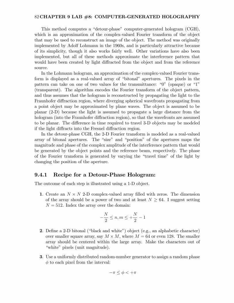
82CHAPTER 9 LAB #8: COMPUTER-GENERATED HOLOGRAPHY
This method computes a �detour-phase� computer-generated hologram (CGH),which is an approximation of the complex-valued Fourier transform of the objectthat may be used to reconstruct an image of the object. The method was originallyimplemented by Adolf Lohmann in the 1960s, and is particularly attractive becauseof its simplicity, though it also works fairly well. Other variations have also beenimplemented, but all of these methods approximate the interference pattern thatwould have been created by light di¤racted from the object and from the referencesource.In the Lohmann hologram, an approximation of the complex-valued Fourier trans-
form is displayed as a real-valued array of �bitonal� apertures. The pixels in thepattern can take on one of two values for the transmittance: �0� (opaque) or �1�(transparent). The algorithm encodes the Fourier transform of the object pattern,and thus assumes that the hologram is reconstructed by propagating the light to theFraunhofer di¤raction region, where diverging spherical wavefronts propagating froma point object may be approximated by plane waves. The object is assumed to beplanar (2-D) because the light is assumed to propagate a large distance from thehologram (into the Fraunhofer di¤raction region), so that the wavefronts are assumedto be planar. The di¤erence in time required to travel 3-D objects may be modeledif the light di¤racts into the Fresnel di¤raction region.In the detour-phase CGH, the 2-D Fourier transform is modeled as a real-valued
array of bitonal apertures. The �size� and �position� of the apertures maps themagnitude and phase of the complex amplitude of the interference pattern that wouldbe generated by the object points and the reference beam, respectively. The phaseof the Fourier transform is generated by varying the �travel time� of the light bychanging the position of the aperture.
9.4.1 Recipe for a Detour-Phase Hologram:
The outcome of each step is illustrated using a 1-D object.
1. Create an N � N 2-D complex-valued array �lled with zeros. The dimensionof the array should be a power of two and at least N � 64. I suggest settingN = 512. Index the array over the domain:
�N2� n;m � +N
2� 1
2. De�ne a 2-D bitonal (�black and white�) object (e.g., an alphabetic character)over smaller square array, say M �M , where M = 64 or even 128. The smallerarray should be centered within the large array. Make the characters out of�white�pixels (unit magnitude).
3. Use a uniformly distributed random-number generator to assign a random phase� to each pixel from the interval:
�� � � < +�

9.4 PROCEDURE: 83
This has the e¤ect of assuming that the re�ecting object (the bitonal character)changes the phase of the incident light by a random angle, and thus approxi-mates a �di¤use�object. The end result is the object function f [n;m].
1-D simulation of detour-phase CGH: (a) bitonal object f [x] consisting of setsof three �bars�; (b) random phase selected from uniform distribution overinterval �� � � < +�; (c) <ff [x]g with random phase; (d) =ff [x]g with
random phase.
4. Compute the FFT F [k; `] of the 2-D �centered�array f [n;m]. Note that youmay have to �checkerboard� (multiply alternate pixels by �1) the array or�torus� it (exchange the quadrants) before and after the FFT, depending onthe FFT algorithm.
5. Compute the magnitude and phase of the 2-D FFT:
jF [k; `]j =q(<fF [k; `]g)2 + (=fF [k; `]g)2
� fF [k; `]g = tan�1�=fF [k; `]g< fF [k; `]g
�, where � � � � < +�
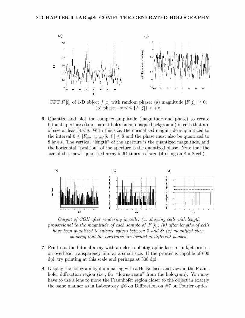
84CHAPTER 9 LAB #8: COMPUTER-GENERATED HOLOGRAPHY
FFT F [�] of 1-D object f [x] with random phase: (a) magnitude jF [�]j � 0;(b) phase �� � � fF [�]g < +�.
6. Quantize and plot the complex amplitude (magnitude and phase) to createbitonal apertures (transparent holes on an opaque background) in cells that areof size at least 8� 8. With this size, the normalized magnitude is quantized tothe interval 0 � jFnormalized [k; `]j � 8 and the phase must also be quantized to8 levels. The vertical �length�of the aperture is the quantized magnitude, andthe horizontal �position�of the aperture is the quantized phase. Note that thesize of the �new�quantized array is 64 times as large (if using an 8� 8 cell).
Output of CGH after rendering in cells: (a) showing cells with lengthproportional to the magnitude of each sample of F [k]; (b) after lengths of cellshave been quantized to integer values between 0 and 8; (c) magni�ed view,
showing that the apertures are located at di¤erent phases.
7. Print out the bitonal array with an electrophotographic laser or inkjet printeron overhead transparency �lm at a small size. If the printer is capable of 600dpi, try printing at this scale and perhaps at 300 dpi.
8. Display the hologram by illuminating with a He:Ne laser and view in the Fraun-hofer di¤raction region (i.e., far �downstream�from the hologram). You mayhave to use a lens to move the Fraunhofer region closer to the object in exactlythe same manner as in Laboratory #6 on Di¤raction on #7 on Fourier optics.
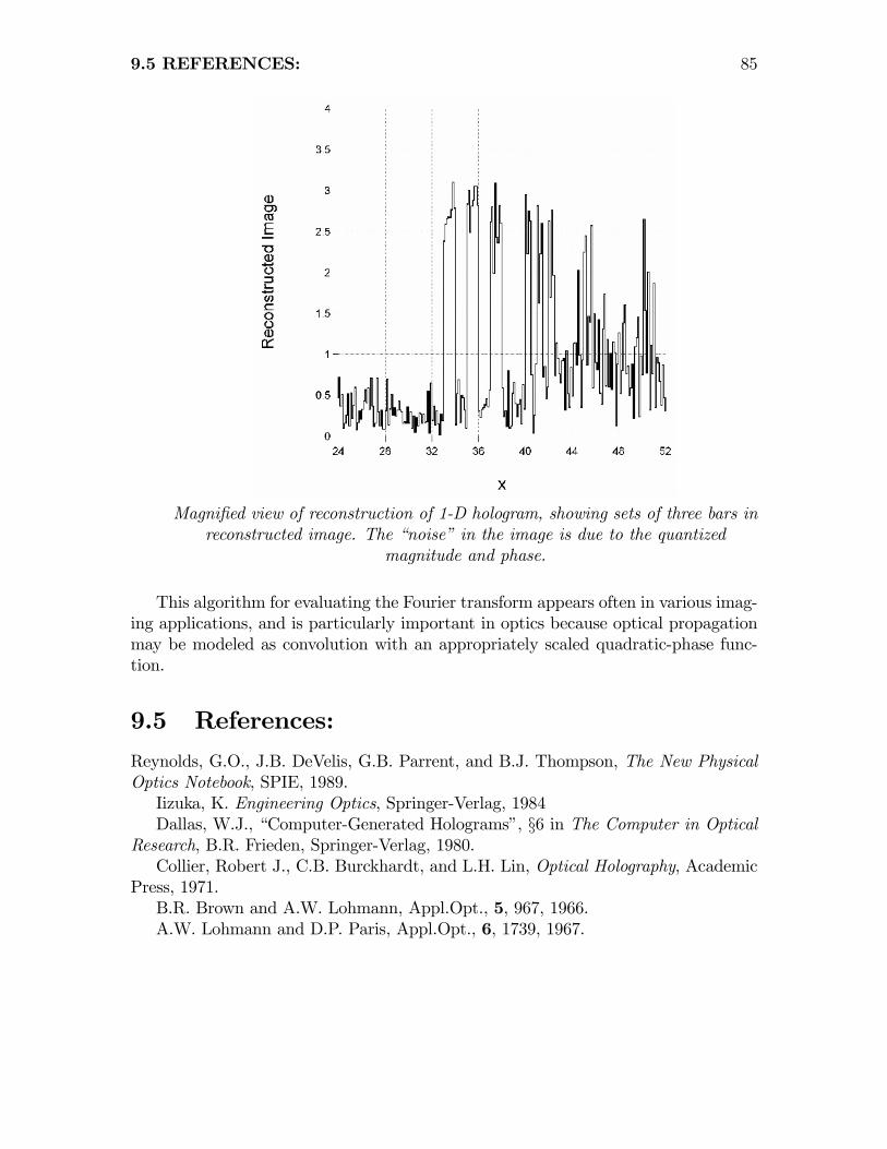
9.5 REFERENCES: 85
Magni�ed view of reconstruction of 1-D hologram, showing sets of three bars inreconstructed image. The �noise� in the image is due to the quantized
magnitude and phase.
This algorithm for evaluating the Fourier transform appears often in various imag-ing applications, and is particularly important in optics because optical propagationmay be modeled as convolution with an appropriately scaled quadratic-phase func-tion.
9.5 References:
Reynolds, G.O., J.B. DeVelis, G.B. Parrent, and B.J. Thompson, The New PhysicalOptics Notebook, SPIE, 1989.Iizuka, K. Engineering Optics, Springer-Verlag, 1984Dallas, W.J., �Computer-Generated Holograms�, §6 in The Computer in Optical
Research, B.R. Frieden, Springer-Verlag, 1980.Collier, Robert J., C.B. Burckhardt, and L.H. Lin, Optical Holography, Academic
Press, 1971.B.R. Brown and A.W. Lohmann, Appl.Opt., 5, 967, 1966.A.W. Lohmann and D.P. Paris, Appl.Opt., 6, 1739, 1967.