10701 recitation: model selection and decision treesaarti/class/10701/recitation/decisiontree... ·...
TRANSCRIPT

10701 Recitation: Decision Trees & Model Selection (AIC & BIC)
Min Chi
Oct 7th, 2010
NSH 1507

More on Decision Trees

Building More General Decision Trees
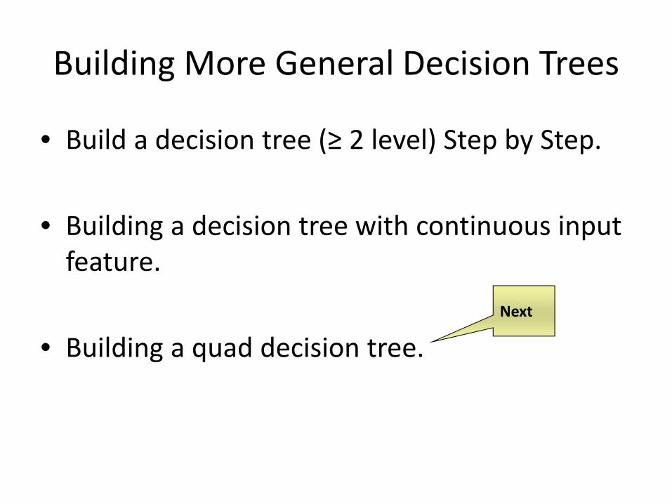
• Build a decision tree (≥ 2 level) Step by Step.
• Building a decision tree with continuous input feature.
• Building a quad decision tree.

Building More General Decision Trees
• Build a decision tree (≥ 2 level) Step by Step.
• Building a decision tree with continuous input feature.
• Building a quad decision tree.
Next

Information Gain• Advantage of attribute – decrease in uncertainty
– Entropy of Y before split
– Entropy of Y after splitting based on Xi• Weight by probability of following each branch
• Information gain is difference
5

How to learn a decision tree
• Top‐down induction [ID3, C4.5, CART, …]
6
Refund
MarSt
TaxInc
YESNO
NO
NO
Yes No
MarriedSingle, Divorced
< 80K > 80K

Person Hair Length
Weight<161
Age<40
Class
Homer Short No Yes MMarge Long Yes Yes F
Bart Short Yes Yes MLisa Long Yes Yes F
Maggie Long Yes Yes FAbe Short No No M
Selma Long Yes No FOtto Long No Yes M
Krusty Long No No M
Comic Long No Yes ?

Short Long
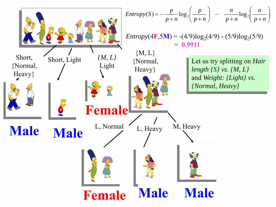
Entropy(4F,5M) = -(4/9)log2(4/9) - (5/9)log2(5/9)= 0.9911
⎟⎟⎠
⎞⎜⎜⎝
⎛++
−⎟⎟⎠
⎞⎜⎜⎝
⎛++
−=np
nnp
nnp
pnp
pSEntropy 22 loglog)(
Gain(Hair Length) = 0.9911 – (3/9 * 0 + 6/9 * 0.9183 ) = 0.3789
)()()( setschildallEsetCurrentEAGain ∑−=
Let us try splitting on Hair length

Weight <161?yes no
Entropy(4F,5M) = -(4/9)log2(4/9) - (5/9)log2(5/9)= 0.9911
⎟⎟⎠
⎞⎜⎜⎝
⎛++
−⎟⎟⎠
⎞⎜⎜⎝
⎛++
−=np
nnp
nnp
pnp
pSEntropy 22 loglog)(
Gain(Weight < 161) = 0.9911 – (5/9 * 0.7219 + 4/9 * 0 ) = 0.5900
)()()( setschildallEsetCurrentEAGain ∑−=
Let us try splitting on Weight

age <= 40?yes no
Entropy(4F,5M) = -(4/9)log2(4/9) - (5/9)log2(5/9)= 0.9911
⎟⎟⎠
⎞⎜⎜⎝
⎛++
−⎟⎟⎠
⎞⎜⎜⎝
⎛++
−=np
nnp
nnp
pnp
pSEntropy 22 loglog)(
Gain(Age < 40) = 0.9911 – (6/9 * 1 + 3/9 * 0.9183 ) = 0.0183
)()()( setschildallEsetCurrentEAGain ∑−=
Let us try splitting on Age

Weight < 161?yes no
Of the 3 features we had, Weight was best. But while people who weigh over 161 are perfectly classified (as males), the under 161 people are not perfectly classified… So we simply recurse!
Male
Person Hair Length
Weight<161
Age<40
Class
Marge Long Yes Yes F
Bart Short Yes Yes M
Lisa Long Yes Yes F
Maggie Short Yes Yes F
Selma Long Yes No F

Entropy(4F,1M) = -(4/5)log2(4/5) - (1/5)log2(1/5)= 0.7219
⎟⎟⎠
⎞⎜⎜⎝
⎛++
−⎟⎟⎠
⎞⎜⎜⎝
⎛++
−=np
nnp
nnp
pnp
pSEntropy 22 loglog)(
Gain(Hair Length, Weight < 161) = 0.7219 – (1/5 * 0 + 3/5 * 0 ) = 0.7219
)()()( setschildallEsetCurrentEAGain ∑−=
Short Long
Let us try splitting on Hair length

Entropy(4F,1M) = -(4/5)log2(4/5) - (1/5)log2(1/5)= 0.7219
⎟⎟⎠
⎞⎜⎜⎝
⎛++
−⎟⎟⎠
⎞⎜⎜⎝
⎛++
−=np
nnp
nnp
pnp
pSEntropy 22 loglog)(
Gain(Age, Weight < 161) = 0.7219 – (3/4 * 0.8113 + 1/4 * 0 ) = 0.1134
)()()( setschildallEsetCurrentEAGain ∑−=
age <= 40?yes no
Let us try splitting on Age

Weight <= 160?yes no
Hair LengthShort Long
Of the 3 features we had, Weight was best. But while people who weigh over 161 are perfectly classified (as males), the under 161 people are not perfectly classified… So we simply recurse!
This time we find that we can split on Hair length and we done.!
Male
FemaleMale

Person Hair Length
Weight<161
Age<40
Class
Homer Short No Yes MMarge Long Yes Yes F
Bart Short Yes Yes MLisa Long Yes Yes F
Maggie Long Yes Yes FAbe Short No No M
Selma Long Yes No FOtto Long No Yes M
Krusty Long No No M
Comic Long No Yes ?

Hair Length
Weight<161
Age<40
Class Count
Short No Yes M 1Long Yes Yes F 3Short Yes Yes M 1Short No No M 1Long Yes No F 1Long No Yes M 1Long No No M 1

Building More General Decision Trees
• Build a decision tree (≥ 2 level) Step by Step.
• Building a decision tree with continuous input feature.
• Building a quad decision tree.
Next

Person Hair Length
Weight<161
Age<40
Class
Homer 0” No Yes MMarge 10” Yes Yes F
Bart 2” Yes Yes MLisa 6” Yes Yes F
Maggie 4” Yes Yes FAbe 1” No No M
Selma 8” Yes No FOtto 10” No Yes M
Krusty 6” No No M

Real‐Values inputWhat should we do if some of the input features are real‐valued?


ExampleHair
Length0” 1” 2” 4” 6” 6” 8” 10” 10”
Class M M M F F M F F MEntropy(4F,5M) = -(4/9)log2(4/9) - (5/9)log2(5/9)
= 0.9911
⎟⎟⎠
⎞⎜⎜⎝
⎛++
−⎟⎟⎠
⎞⎜⎜⎝
⎛++
−=np
nnp
nnp
pnp
pSEntropy 22 loglog)(

ExampleHair
Length0” 1” 2” 4” 6” 6” 8” 10” 10”
Class M M M F F M F F M

However,…
• Gain(Hair Length < 4’’) = 0.9911 – (3/9 * 0 + 6/9 * 0.9183 ) = 0.3789
• Gain(Weight < 161) = 0.9911 – (5/9 * 0.7219 + 4/9 * 0 ) = 0.5900
• Gain(Age < 40) = 0.9911 – (6/9 * 1 + 3/9 * 0.9183 ) = 0.0183

Weight < 161?yes no
Of the 3 features we had, Weight was best. But while people who weigh over 160 are perfectly classified (as males), the under 160 people are not perfectly classified… So we simply recurse!
Male
Person Hair Length
Weight<161
Age<40
Class
Marge 10” Yes Yes F
Bart 2” Yes Yes M
Lisa 6” Yes Yes F
Maggie 4” Yes Yes F
Selma 8” Yes No F

ExampleHair
Length2” 4” 6” 8” 10”
Class M F F F FEntropy(4F,1M) = -(4/5)log2(4/5) - (1/5)log2(1/5) = 0.7219
Gain(Hair Length < 4’’, Weight < 161) = 0.7219 – (1/5 * 0 + 4/5 * 0 ) = 0.7219
Gain(Age, Weight < 161) = 0.7219 – (3/4 * 0.8113 + 1/4 * 0 ) = 0.1134

Weight < 161?yes no
Hair Length < 4?yes no
Of the 3 features we had, Weight was best. But while people who weigh over 160 are perfectly classified (as males), the under 160 people are not perfectly classified… So we simply recurse!
This time we find that we can split on Hair length, and we are done!
Male
Male Female

Building More General Decision Trees
• Build a decision tree (≥ 2 level) Step by Step.
• Building a decision tree with continuous input feature.
• Building a quad decision tree. Next
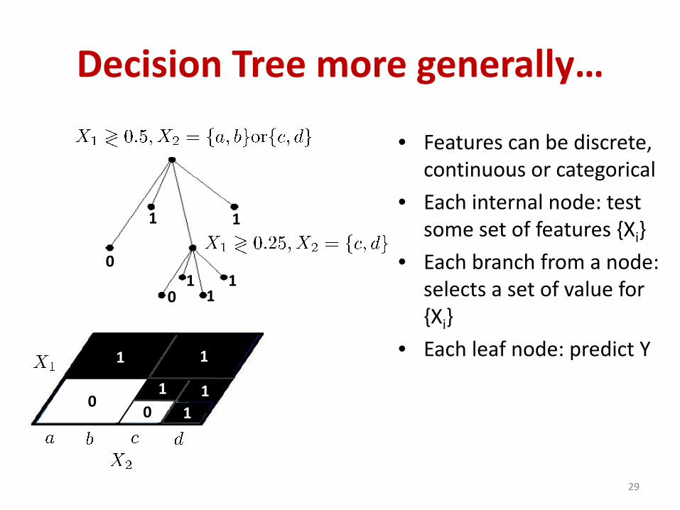
Decision Tree more generally…
29
1 1
10
10
• Features can be discrete,continuous or categorical
• Each internal node: test some set of features {Xi}
• Each branch from a node: selects a set of value for {Xi}
• Each leaf node: predict Y
1
11
01 1
10

Person Hair Length
Weight Class
Homer 0” 250 MMarge 10” 150 F
Bart 2” 90 MLisa 6” 78 F
Maggie 4” 20 FAbe 1” 170 M
Selma 8” 160 FOtto 10” 180 M
Krusty 6” 200 M
Hair length:0‐2 Short3‐6 Medium≥7 Long
Weight:0‐100 Light100‐175 Normal≥175 Heavy

Person Hair Length
Weight Class
Homer S Heavy MMarge L Normal F
Bart S Light MLisa M Light F
Maggie M Light FAbe S Normal M
Selma L Normal FOtto L Heavy M
Krusty M Heavy M
Hair length:0‐2 Short3‐6 Medium≥7 Long
Weight:0‐100 Light100‐175 Normal≥175 Heavy

Short, {Normal, Heavy}
Entropy(4F,5M) = -(4/9)log2(4/9) - (5/9)log2(5/9)= 0.9911
⎟⎟⎠
⎞⎜⎜⎝
⎛++
−⎟⎟⎠
⎞⎜⎜⎝
⎛++
−=np
nnp
nnp
pnp
pSEntropy 22 loglog)(
Let us try splitting on Hair length {S} vs. {M, L}and Weight: {Light} vs. {Normal, Heavy}
Short, Light {M, L}Light
{M, L}{Normal, Heavy}

{M, L} * {Normal, Heavy}Let us try re-splitting on Hair length: M vs. Land Weight: Normal vs. Heavy
L, Normal L, Heavy M, NormalM, Heavy
Short, {Normal, Heavy}
Entropy(4F,5M) = -(4/9)log2(4/9) - (5/9)log2(5/9)= 0.9911
⎟⎟⎠
⎞⎜⎜⎝
⎛++
−⎟⎟⎠
⎞⎜⎜⎝
⎛++
−=np
nnp
nnp
pnp
pSEntropy 22 loglog)(
Let us try splitting on Hair length {S} vs. {M, L}and Weight: {Light} vs. {Normal, Heavy}
Short, Light {M, L}Light
{M, L}{Normal, Heavy}
L, Normal L, Heavy M, Heavy
FemaleMale Male
Male MaleFemale

Short, Weight ≥161
Entropy(4F,5M) = -(4/9)log2(4/9) - (5/9)log2(5/9)= 0.9911
⎟⎟⎠
⎞⎜⎜⎝
⎛++
−⎟⎟⎠
⎞⎜⎜⎝
⎛++
−=np
nnp
nnp
pnp
pSEntropy 22 loglog)(
Let us try splitting on Hair length {S} vs. {M, L}and Weight: {Light} vs. {Normal, Heavy}
Short, Weight ≥161
Long, Weight < 161
Long, Weight ≥161
Short, {Normal, Heavy}
Short, Light {M, L}Light
{M, L}{Normal, Heavy}
FemaleMale

Model and Selection: AIC & BIC

Bias, Variance, and Model Complexity
•Bias‐Variance trade‐off again
•Generalization: test sample vs. training sample performance
– Training data usually monotonically increasing performance with model complexity

Measuring Performance
•target variable •Vector of inputs •Prediction model
•Typical Choices of Loss function
( )( ) ( )( )( )
2ˆˆ,
ˆ
Y f X squared errorL Y f X
Y f X absolute error
⎧ −⎪= ⎨⎪ −⎩
YX( )f X

• Test error aka. Generalization error
• Note: This expectation averages anything that is random, including the randomness in the training sample that it produced
• Training error
•– average loss over training sample
– not a good estimate of test error (next slide)
( )( )ˆ,Err E L Y f X⎡ ⎤= ⎣ ⎦
( )( )1
1 ˆ,n
i ii
err L y f xN =
= ∑
Generalization Error

Training Error
•Training error ‐ Overfitting– not a good estimate of test error
– consistently decreases with model complexity
– drops to zero with high enough complexity

Categorical Data•same for categorical
responses
•
•Typical Choices of Loss functions:
( ) ( )|kp X pr G k X= =
( ) ( )ˆ ˆarg maxk kG X p X=
( )( ) ( )( )ˆ ˆ, 0 1 L G G X I G G X loss= ≠ −
( )( ) ( ) ( ) ( )1
ˆ ˆ ˆ, 2 log 2 log logK
k Gk
L G p X I G k p X p X likelihood=
= − = = − −∑Log‐likelihood = cross‐entropy loss = deviance
)(ˆlog21
i
N
ig xp
Nerr
i∑=
−=
Training Error again:
Test Error again:
))](ˆ,([ xpGLEErr =

with predictor ( ) ( )Pr X Yθ Ydensity of X
Loss Function for General Densities
• For densities parameterized by theta:
• Log‐likelihood function can be used as a loss‐function
( )( ) ( ) ( ), 2 log Pr XL Y X Yθθ = −

Two separate goals
• Model selection:– Estimating the performance of different models in order to choose the
(approximate) best one
• Model assessment:– Having chosen a final model, estimating its prediction error (generalization
error) on new data
• Ideal situation: split data into the 3 parts for training, validation (est. prediction error+select model), and testing (assess model)
• Typical split: 50% / 25% / 25%
• Remainder of the chapter: Data‐poor situation• => Approximation of validation step either analytically (AIC, BIC, MDL,
SRM) or by efficient sample reuse (cross‐validation, bootstrap)
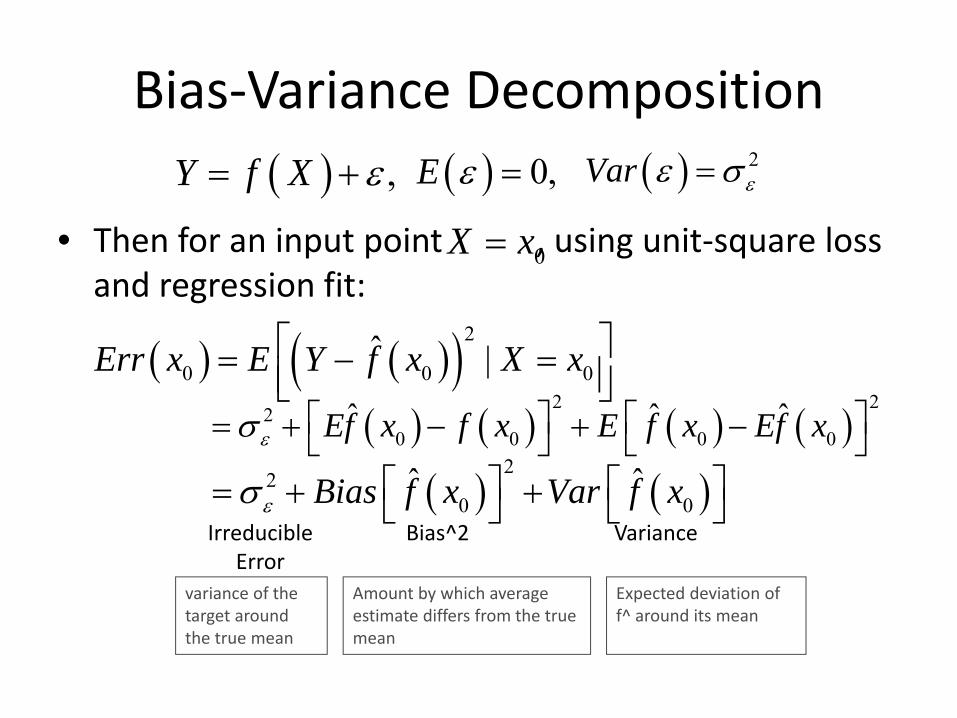
Bias‐Variance Decomposition
• Then for an input point , using unit‐square loss and regression fit:
( ) ,Y f X ε= + ( ) 0,E ε = ( ) 2Var εε σ=
0X x=
( ) ( )( )2
0 0 0ˆ |Err x E Y f x X x⎡ ⎤= − =⎢ ⎥⎣ ⎦( ) ( ) ( ) ( )
2 22
0 0 0 0ˆ ˆ ˆEf x f x E f x Ef xεσ ⎡ ⎤ ⎡ ⎤= + − + −⎣ ⎦ ⎣ ⎦
( ) ( )2
20 0
ˆ ˆBias f x Var f xεσ ⎡ ⎤ ⎡ ⎤= + +⎣ ⎦ ⎣ ⎦Irreducible
ErrorBias^2 Variance
variance of the target around the true mean
Amount by which average estimate differs from the true mean
Expected deviation of f^ around its mean

Bias‐Variance Decomposition( ) ( ) ( )
22
0 0 0ˆ ˆErr x Bias f x Var f xεσ ⎡ ⎤ ⎡ ⎤= + +⎣ ⎦ ⎣ ⎦
kNN: ( ) ( ) ( )( )2
2 20
1
1 /k
o ll
Err x f x f x kkε εσ σ
=
⎡ ⎤= + − +⎢ ⎥⎣ ⎦∑
Linear Model Fit: ( )ˆ ˆTpf x xβ=
( ) ( ) ( ) ( )2 22 2
0 0 0ˆ
o pErr x f x Ef x h xε εσ σ⎡ ⎤= + − +⎣ ⎦
( ) ( ) 1
0where h x T TX X X y−
=

Bias‐Variance Decomposition
Linear Model Fit: ( )ˆ ˆTpf x xβ=
( ) ( ) ( ) ( )2 22 2
0 0 0ˆ
o pErr x f x Ef x h xε εσ σ⎡ ⎤= + − +⎣ ⎦
( ) ( ) 1
0where h x ... N-dim weight vectorT TX X X y−
=
iaverage over sample values x :
( ) ( ) ( )2
2 2
1 1
1 1 ˆ ... in-sample errorN N
i i ii i
pErr x f x Ef xN N Nε εσ σ
= =
⎡ ⎤= + − +⎣ ⎦∑ ∑
Model complexity is directly related to the number of parameters p

Bias‐Variance Decomposition( ) ( ) ( )
22
0 0 0ˆ ˆErr x Bias f x Var f xεσ ⎡ ⎤ ⎡ ⎤= + +⎣ ⎦ ⎣ ⎦
For ridge regression and other linear models, variance same as before, butwith diff’t weights.
( )( )2
* arg min TE f X Xβ
β β= −Parameters of the best fitting linear approximation
Further decompose the bias:
200*
20*0
200 ][])([)](ˆ)([
000xExExxfExfExfE TT
xT
xx αα βββ −+−=−22 ]Bias Estimation[]Bias Model[ AveAve +=
Least squares fits best linear model ‐> no estimation biasRestricted fits ‐> positive estimation bias in favor of reduced variance

Optimism of the Training Error Rate
• Typically: training error rate < true error
• (same data is being used to fit the method and assess its error)
( )( )ˆ,Err E L Y f X⎡ ⎤= ⎣ ⎦( )( )1
1 ˆ,n
i ii
err L y f xN =
= ∑ <
overly optimistic

Optimism of the Training Error RateErr … kind of extra‐sample error: test features don’t need to coincide with training feature vectors
Focus on in‐sample error: ( )( )1
1 ˆ,new
Nnew
in Y i iYi
Err E E L Y f xN =
= ∑
newY … observe N new response values at each of training points , i=1, 2, ...,Nix
( )optimism: in yop Err E err≡ −
for squared error 0‐1 and other loss functions: ( )1
2 ˆ ,N
i ii
op Cov y yN =
= ∑
iThe amount by which err underestimates the true error depends on how strongly y affects its own prediction.
Optimism of the Training Error Rate
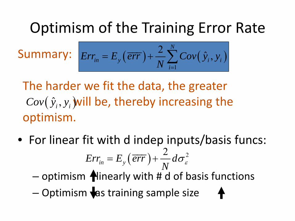
Summary: ( ) ( )1
2 ˆ ,N
in y i ii
Err E err Cov y yN =
= + ∑
The harder we fit the data, the greater will be, thereby increasing the
optimism. ( )ˆ ,i iCov y y
• For linear fit with d indep inputs/basis funcs:
– optimism linearly with # d of basis functions
– Optimism as training sample size
( ) 22in yErr E err d
N εσ= +

Optimism of the Training Error Rate
• Ways to estimate prediction error:– Estimate optimism and then add it to training error rate
• AIC, BIC, and others work this way, for a special class of estimates that are linear in their parameters
– Direct estimates of the sample error • Cross‐validation, bootstrap
• Can be used with any loss function, and with nonlinear, adaptive fitting techniques
•
err
Err

Estimates of In‐Sample Prediction Error
• General form of the in‐sample estimate:
• For linear fit and with : ( ) 22in yErr E err d
N εσ= +
22 ˆ , so called statisticp pdC err C
N εσ= +
2ˆ ... estimate of noise variance, from mean-squared error of low-bias modelεσ
... # of basis functionsd... training sample sizeN
poerrin ˆrrE += with estimate of optimism

Estimates of In‐Sample Prediction Error
• Similarly: Akaike Information Criterion (AIC)– More applicable estimate of , when log‐likelihood function is used
inErr
( ) [ ]ˆ2For : 2 log Pr log lik 2 dN E Y EN Nθ
⎡ ⎤→∞ − ≈ − +⎣ ⎦
( )
( )ˆ1
Pr ... family density for Y (containing the true density)ˆ... ML estimate of
loglik= log PrN
ii
Y
y
θ
θ
θ θ
=∑ Maximized log‐likelihood due to ML
estimate of theta

AIC
( ) [ ]ˆ2For : 2 log Pr log lik 2 dN E Y EN Nθ
⎡ ⎤→∞ − ≈ − +⎣ ⎦
For example, for logistic regression model, using binomial log‐likelihood:
To use AIC for model selection: choose the model giving smallest AIC over the set of models considered.
( ) ( ) ( ) 2ˆ2d
AIC errN ε
αα α σ= +
( )( ) ( )
ˆ ... set of models, ... tuning parameter
err ... training error, ... # parameters
f x
dα α
α α
Nd
NAIC ⋅+⋅−= 2loglik2

AIC
• Function AIC(α) estimates test error curve• If basis functions are chosen adaptively with d<p inputs:
• no longer holds => optimism exceeds
• effective number of parameters fit > d
2
1
),ˆ( εσdyyCov i
N
ii =∑
=
2)/2( εσNd

Using AIC to select the # of basis functions
• Input vector: log‐periodogram of vowel; Quantized to 256 uniformly spaced f
• Linear logistic regression model • Coefficient function:
– Expansion of M spline basis functions– For any M, a basis of natural cubic splines is used for the knots chosen uniformly over the range of frequencies, i.e.
• AIC approximately minimizes Err(M) for both entropy and 0‐1 loss
•
( ) ( )1
M
m mm
f h fβ θ=
=∑
mh( ) ( )d d M Mα = =
( ) 2
1
2 2ˆ , ... simple formula for linear caseN
i ii
dCov y yN N εσ
=
=∑

Using AIC to select the # of basis functions
( ) 2
1
2 2ˆ ,N
i ii
dCov y yN N εσ
=
=∑
Approximation does not hold, in general, for 0‐1 case, but it does o.k. (Exact only for linear models w/ additive errors and sq err loss)

Effective Number of Parameters1
2
y
y=
N
y
y
⎛ ⎞⎜ ⎟⎜ ⎟⎜ ⎟⎜ ⎟⎜ ⎟⎝ ⎠
MVector of Outcomes, similarly for predicitons
y Sy= Linear fit (e.g. linear regression, quadratic shrinkage – ridge, splines)
i i... N N matrix, depends on input vector x but not on yS ×
( ) ( )effective number of parameters: d S trace S=
22 ˆpdC err
N εσ= +
c.f. ),ˆ( yyCov
d(s) is the correct d for Cp

Bayesian Approach and BIC
• Like AIC used in when fitting by max log‐likelihood
BIC proportional to AIC except for log(N) rather than factor of 2. For N>e2 (approx 7.4), BIC penalizes complex models more heavily.
Bayesian Information Criterion (BIC):
])(log[then
//))(ˆ(loglik2
known, :modelGaussian Assuming
22
222
2
εε
εε
ε
σσ
σσ
σ
NdNerrNBIC
errNxfyi ii
⋅+=
⋅=−≈⋅− ∑
dNCBI )(logloglik2 +−=

BIC Motivation
• Given a set of candidate models
• Posterior probability of a given model:
• Where
• To compare two models, form the posterior odds:
• If odds > 1, then choose model m. Prior over models (left half) considered constant. Right half, contribution of data (Z) to posterior odds, is called the Bayes factor BF(Z).
• Need to approximate Pr(Z|Mm). Various chicanery and approximations (pp. 207) gets us BIC.
• Can est. posterior from BIC and compare relative merits of models.
m parameters model and 1, θMmm K=Μ)|Pr()Pr()|Pr( mmm MZMZM ⋅∝
Nii yx 1},{ data training therepresents Z
)|Pr()|Pr(
)Pr()Pr(
)|Pr()|Pr(
l
m
l
m
l
m
MZMZ
MM
ZMZM
⋅=

BIC: How much better is a model?• But we may want to know how various models stack up (not just ranking) relative
to one another:
• Once we have the BIC:
• Denominator normalizes the result and now we can assess the relative merits of each model
∑ =
⋅−
⋅−
≡M
l
BIC
BIC
ml
m
e
e
121
21
)|Pr( of estimate ZM