ILE COPY

NATIONAL ADVISORY COMMITTEE FOR AERONAUTICS

1111-IRTIM11 R111PORT ORIGINALLY ISSUED

November 1943 as Advance Restricted Report 3K02

THE FLOW OF A COMPRESSIBLE FLUID PAST

A CURVED SURFACE

By Carl Kaplan

Langley Memorial Aeronautical Laboratory Langley Field, Va.

FILE COpy TOt*returndt.

t files of the NtisnaJ Advisory Comnflj

for Airormutjc

NACA WASHINGTON

NACA WARTIME REPORTS are reprints of papers originally Issued to provide rapid distribution of advance research results to an authorized group requiring them for the war effort. They were pre-viously held under a security status but are now unclassified. Some of these reports were not tech-nically edited. All have been reproduced without change In order to expedite general distribution.

L - 32

https://ntrs.nasa.gov/search.jsp?R=19930093633 2019-08-29T12:36:40+00:00Z

NATIONAL ADVISORY CO?I1ITTEE FOR AERONAUTICS

ADVANCE RESTRICTED REPORT S

THE FLOW OF A COMPRESSIBLE FLUID PAST

A CURVED SURFACE

By Carl Kaplan

SUMMARY

An iteration method is employed- -to obtain the flow of a com-pressible fluid past a curved surface. The first apnroximation, which leads to the Prandtl-Glauert rule, is based on the assumption that the flow differs but little from a pure translation. The iteration process then consists in improving this first approxi-mation in order that it will apply to a flow differing from pure translatory motion to a greater degree. The method fails when the Mach number of the undisturbed stream reaches unitybt permits a transition from subsonic to supersonic conditions without the ap-pearance of a compression shock. The limiting value of the undisturbed stream Mach number, defined as that value at which potential flow no longer exists, is indicated by the apparent dir. vergence of the power series representing the velocity of the fluid at the surface of the solid boundary.

For small c.h numbers and for thin shapes, the results ob-tained by the iteration process agree with those obtained by the Poggi method. For highr values of the streai Mach number less than the critical value, numerical calculations are in agreement with the results obtained by von Krm6'n by means of the hodograph method. For values of the stream Mach number higher than' the critical value, the iteration process yields some information about the region of flow comprised between the critical stream Mach num-ber and the limiting stream Mach number.

INTRODUCTION

When a body is' held fired in a compressible fluid moving at a uniform speed less than, but comparable with, that of sound, there may be a region near the surface where the velocity of the fluid relative to the body exceeds the local velocity of sound. The flow in such cases may be perfectly regular with no indication of shock waves. Several such types of flow have been described by Taylor

(reference 1) and, more recently, by Görtler (reference 2). In con-

nection with this type of flow it is important to know when the ir-

rotational motion ceases to be possible. It is certain that ir-

rotational motion is no longer possible as soon as the Mach number of the undisturbed stream reaches a definite value, always less than unity, which depends on the shape of the body. In the past com-

pressibility shock has often been assumed to occur when the maximum velocity of the fluid at the surface of the body equals the local velocity of sound; however, the papers of Taylor and Görtler (ref-erences 1 and 2) question whether this is correct for the first ap-pearance of a shock wave. In addition, a recent paper by von Krmn

(reference 3) suggests that the envelope of the Mach lines in the supersonic region of flow probably introduces the first shock wave in the flow. The stream Mach number at which the envelope of the Mach lines first appears ma thus be identified with a limiting

value of the Mach number.

The present paper treats the flow of a compressible fluid past a- curved surface by means of an iteration process based on that of Ackeret (reference 4). The boundary was so chosen as to conform with the requirements of the method; namely, no stagnation points and small variation of the local velocity from that in the stream. The process, furthermore, permits values of the stream Mach number ranging from zero to the neighborhood of unity. The method proves

to be quite laborious when more than two stages in the iteration are demanded; but, because of the importance of the problem, it has been thought worth while to perform the third step. Most of the details of the calculations have been relegated to appendixes in order not to disturb the continuity of the main ideas. (The equations in the appendixes have been assigned numbers prefixed by letters denoting the appendix; for example, equation (A-3) is the third equation in appendix A.)

THE ITERATION PROCESS

The fundamental differential equabion governing the flow of a compressible fluid is

/2- U 2\ÔU (2 fv u

(1) uv—+-- -

- -o

where

X, Y rectangular Cartesian coordinates in plane of profile

3

U P V fluid velocity components along X and .1 axes

c local velocity of cund.

The condition for irrotational motion is that

àu ày

6Y 6X

and leads to a velocity potential 0 defined by

U*1(2)

Cy

0

If the body is held fixed in a uniform stream of velocity U, the relation between the local velocity of sound c and the velocity of

the fluid V97 v2_ is given for adiabatic processes by

=1+ '-'-.2 u2co 2 )(3)

where

co velocity of sound in undisturbed stream

ratio of specific heats at constant pressure and constant volume

M !ch number of undisturbed stream (U/c0)

With 'the introduction of a characteristic length s. as unit of length and the stream velocity U as unit of velocity, the various quantities thus far defined can 'be rendered nondimensional. Thus

X,. Y, u, v, and denote, respectively, the nondimonsional quantities X/s. Y/s, u/U, v/U, and 0/us while c and c0

retain their original meanings. By use of equation. (2), equa-

tions (1) and (3) then become, respectively, '

14

C2 CO22' 21 0 (14)

co

2 Jàx c2 / 6y2 àXàYàXÔY

and

02 (2 (5)

Let t denote a characteristic parameter of the shape, such as

the thickness coefficient; then, the .followin expansions are as-

sumed:

6X 6Xa

(6) oø'l aø'2

by by ày. by

When these expressions for u and v are introd uced into equa-

tion (14), together with the expression for given by equa-

tion (5), and when the coefficients of the various powers of t are

equated to zero, the following differential equations for

03i • • . result:

à20•1 a20'i + = 0

ax2 C) y2

a202 a20 ____ aøl øl àØ1 e201 (i_i) .i. = L (y^1) - . + (y_f .- .+ 2— (.8)

ax2 ày2. ax 6 X ' ax ày' by àXàY

(7)

5

(i -) o20 + a2 [ 2 1

2 + (y-1).

6x2 y2 12X, L a- aY-J

ll\2

2 1)à2øl + (p1) 1

L

2V6 Y/

a' — . ___ + j(y+l)-'--.--- +.

axL ax2 ay2j

- + -- I(+l)- + ( y-l) 2

x L

+21 2 2)

(9) ax àY a xàY àY àxà'r àY a xàY

These differential equations may be put into more familiar forms by introducing a new, set of independeit variables x and where

x I

• (10)

y 4 - 1•Y J

Thus, for TBA < 1, equation (7) is transformed into a Laplace equa-tion and equations (8) and (9) into Poisson equations. The solu-tion of equation (7) yields the well-known PraxcIt1-Glauert rule,

whereas the solutions of equations (8) and (9) provide higher ap-proximations to the flow of a compressible fluid and thus will ap-

ply for larger departures from an undisturbed uniform flow..

The procedure to be followed in solving equations (7), (8), and

(9) is very simple in principle. The first step is to obtain an expression for the velocity potential of the incompressible flow past the chosen boundary and to express it as a power series iii the thickness coefficient t. Then the solution for the first approxi-

mation Ø to the compressible flow is e&sily obtained by analogy

from the coefficient of the first power of t. The second and

third approxlma.tions '2 andare obtained by solving equa-

tions (8) and (9) . The boundary conditions - that the flow is tangential to the solid boundary and that the disturbance to the main flow vanishes at infinity - aresatisfied to the same power of the thickness coefficient t which is involved in the expression for the velocity potential 0.

Flow past a Curved Surface

The solid boundary chosen for use in this paoer is a symmetri-cal shaoe with cusps at both the leading and the trailing edges, thus insuring no stagnation points in a uniform flow parallel to the axis of symmetry. Appendix A contains the derivation of this shape and also the solution for the flow of an incompressible fluid

past it. Appendixes 13, C, and D contain the detailed calculations

for 02, and Ø, respectively. The final expression for the

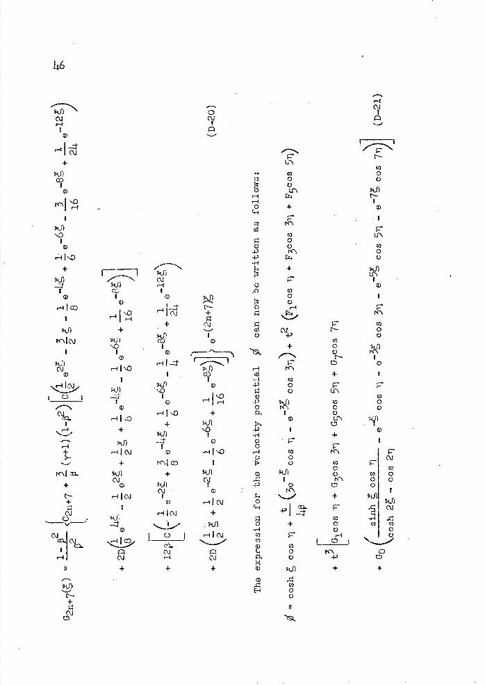
velocity potential 0 takes he .following form:

0 cosh + _(3e cos i - e cos cos i

• t2 (F3 cos r + F3 cos 31i + F5 cos 5T))

• cos 71 + 03 cos 3 + G5 cos 51i + G7 cos 711

( sinh, cos 1)-

\cosh 2, - cos 2q

- C COS 7T) + .. • •

r ecos i - e_cos 3q - e cos

(ii)

7

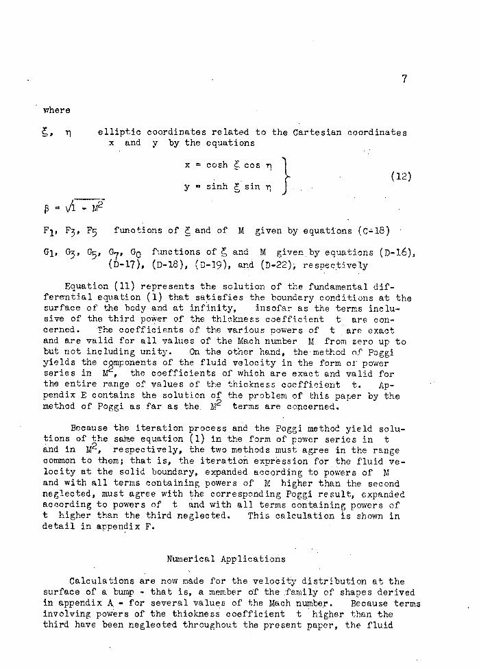
where

T) elliptic coordinates related to the Cartesian coordinates x and y by the equations

x cosh cos(12)

ysinhsin r, J..

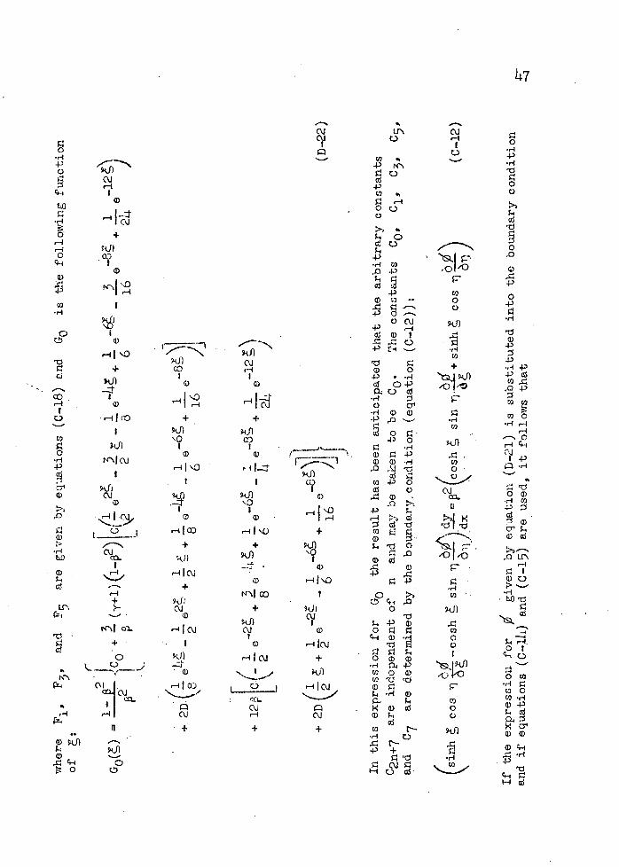
F1, F3, F5 functions of and of M given by equations (c18)

G1, G3, G5, G7, G0 functions of , and M given by equations (D-l6),

( D-l7), (n-iS), (0-19), and (D-22) respectively

Equation (11) represents the solution of the fundamental dif-ferential equation (1) that satisfies the boundary conditions at the surface of the body and at infinity, insofar as the terms inclu-

sive of the third power of the thickness coefficient t are con-cerned. The coefficients of the various powers of t are exact and are valid for all values of the Mach number M from zero up to but not including unity. On the other hand, the method of Poggi yields the cmponents of the fluid velocity in the form or power series in M, the coefficients of which are exact and valid for the entire range of values of the thickness coefficient t. Ap-

pendix E contains the solution of the problem of this paper by the method of Poggi as far as the. terms are concerned.

Because the iteration process and the Poggi method yield solu-tions of the same equation (1) in the form of power series in t and in M2, respectively, the two methods must agree in the range common to them; that is, the iteration expression for the fluid ve-locity at the solid boundary, expanded according to powers of M and with all terms containing powers of M higher than the second neglected, must agree with the corresponding Poggi result, expanded according to powers of t and with all terms containing powers of t higher than the third neglected. This calculation is shown in detail in ap pendix F.

Numerical Applications

Calculations are now made for the velocity distribution at the surface of a bump - that is, a member of the :family of shapes derived in appendix A - for several values of the Mach number. Because terms involving powers of the thickness coefficient t higher than the third have been neglected throughout the present paper, the fluid

8

velocity . q should be expressed in the following form:

q 1 + alt + a2t2 + a3 t3 + . (13)

From equations (F- 6) it follows easily that

= - --- cos 2a 2

a2

1)(

___ 9.

1 P_ + _L_ -+ cos 2a 2 J 8p2 16 4I3

+ '1) 2+ 3 6 +. op - 3

L216 2 1

> . (iL') a3 =, - + (1 + 3Q7 + 5G5 + 7)

. I

0 .

16

+ - lp) + 2(3G3 + 5G5 cos 2a L64 32 -

+ [

9

+ 5P + 3P2 2(5G5 .+ 7G] cos 4a

16 P7)0

+ 82p ^.2cos 6a L . 0_.

The expressions for ccrl), ('G 0 (G5)0 and (G70 are given at

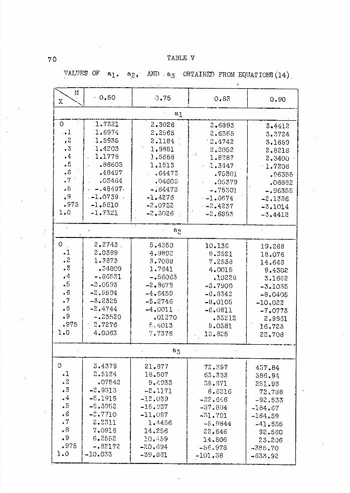
the end of appendix F, and table IV shows the calculated values for M 0.50, 0.75, 0.83, and 0.90. Table V gives the calculated values of a1 , a2, and a3 'at various positions along the profile

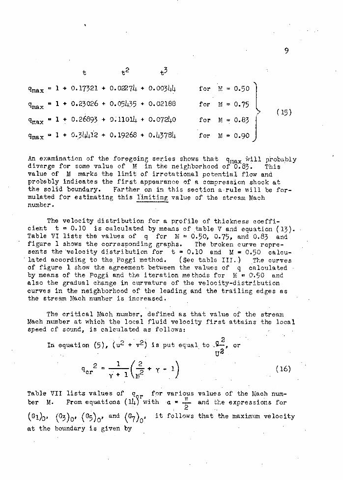
for M 0 .5 0 , '0 .75, 0.83, and 0.90. With t 0.10, the expres-sions-for the maximum fluid velocity q at the surface can be max written as follows:

for M 0.50

for M = 0.75

for lv! = 0.83

for M 0.90

('5)

9

t t2 t3

qmax = 1 + 0.17321 + 0.074 + 0.003414

1 + 0.23026 + 0.05435 + 0.02183

qmax 1 + 0.26893 + 0.110114 + 0.07240

q x 1 + O. 3L 1412 + 0.19268 + 0.3784

An examination of the foregoing series shows thatq-m x *ill piobahly diverge for some value of M in the neighborhood of 0.83. This value of M marks the limit of irrotational potential flow and probably indicates the first appearance of a compression shock at the solid boundary. Farther on in this section arule will be for-

mulated for estimating this limiting value of the stream Mach number.

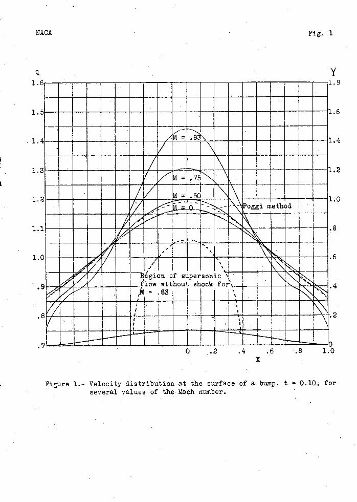
The velocity distribution for a profile of thickness coeffi-cient t 0.10 is calculated by means of table V and equation (13). Table VI lists the values of q for Iv! = 0.50, 0.75, and 0.83 and figure 1 shows the corresponding graphs. The broken curve repre-sents the velocity distribution for t 0.10 and M * 0. 50 calcu-lated according to the Poggi method. (See table III.) The curves of figure 1 show the agreement between the values of q calculated by means of the Poggi and the iteration methods for M = 0.50 and also the gradual change in curvature of the velocity-distribution curves in the neighborhood of the leading and the trailing edges as the stream Mach number is increased.

The critical Mach number, defined as that value of the stream Mach number at which the local fluid velocity first attains the local speed of sound, is calculated as follows:

In equation (5), (u2 + v2 ) is put equal to

or U2.

q 2= 1 or

Table VII lists values of q r for various values of the Mach num- Tr ber M. From equations (1)4 with a = and the expressions for

(16)

(Gi)0, (G3) 0 (G5) 01 and (G7 )01 it follows that the maximum velocity

at the boundary is given by

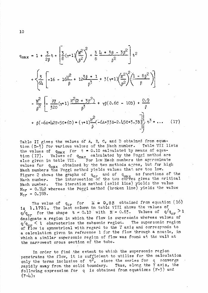
10

3 '3M2 qmax 1 + t (i)(

2P 2

+ 16 16— + 12

3 P t2

6_j

+ (^2

2/'\ i

M(2 + 382) + 1 (0.6c - 10D) + 22

2 320 3

1 + (-6A+42B-5c+6D) + (i)-(-6A+33B-2.145 C+3 . 3 D) t3 + ... (17)

Table II gives the values of A, B, C, and D obtained from ecia-tion (D-3) for various values of the Mach number. Table VII lists

the values of qjrax for t 0.10 calculated by means of equa-

tion ( 17) . Values of qrria7 calculated by the Poggi method are

also given in table VII. For low Mah numbers the approximate values for q1 obtained by the two, methods arree, but for high Mach numbers the Poggi method yields values that are too low. Figure 2 shows the graphs of qcr and of qmax as functions of' the Mach number. The intersection of the two curves gives the critical Mach number. The iteration method (solid line) yields the value Mer 0.742 whereas the Poggi method (broken line) yields the value Mcr 0.788.

The value of qcr for = 0.83 obtained from equation (16) is 1.1731. The last column in table VIII shows the values of

q/q for the shape t 0.10 with M= 0.83. Values of /q0 >1

designate a region in which the flow is supersonic whereas values of q/qcr < 1 characterize the subsonic region. The supersonic region

of flow is s ymmetrical with regard to the Y axis and corresponds to a calculation given in reference 1 for the flow through a nozzle, in which a similar supersonic region' of flow was found at the wall at the narrowest cross section of the tub.

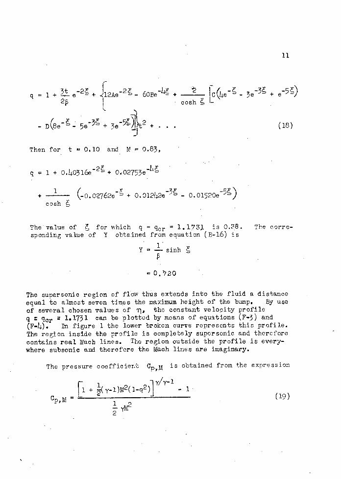
In order to find the extent to which the supersonic region penetrates the flow, it is sufficient to utilize for the calculation only the terms inclusive of t'-, since the series for .q converge rapidly away from the solid boundary. Thus, along the Y axis, the

following expression for q is obtained from equations ( F-3) and

11

q 1 + e2 + J2Ae2 - 60Be + [c(e - 3e + 2 L cosh

- D(8e- 5e + 3e 52 +

Then for t 0.10 and N = 0.83,

q = 1 + 0. L0316e_ 2 + 0.02753e -Ii

1 + (_0.O2762e + 0.012142e 3 - 0.01520e5)

cosh

The value of for which q = q0 1.1731 is 0.38. The corre-sponding value of Y obtained from equation (B-16) is

Y -.- sinh

= 0.20

The supersonic region of flow thus extends into the fluid a distance equal to almost seven times the maximum height of the bump. By use of several chosen values of In, the constant velocity profile q 1-1731 can be plotted by means of equations (F-3) and (F-Li.). In figure 1 the lower broken curve represents this profile. The region inside the profile is completely su personic and therefore contains real Mach lines. The region outside the profile is every-where subsonic and therefore the Mach lines are imaginary.

The pressure coefficient CpM is obtained from the expression

.1 y/y-1 1' + ( yl)M2(lq2)j - 1(19)

1YI

(18)

12

- where

p - p0

1- p0tJ

and q is the velocity of the compressible fluid, referred to the velocity U of the undisturbed stream.

Since, throughout this paDer, terms involving powers of: t higher than the third have been neglected, Cn,M should be expressed as a power series in t. Thus, if q from equation (13) is sub-stituted into equation (19), it follows easily that

Cp, M -2a 1t + (a 12 + 2a2 ) + a i2M2 t2

+E2(aia2+ az) + (a 2 +2a )ai2 ai3H t + . . . (20)

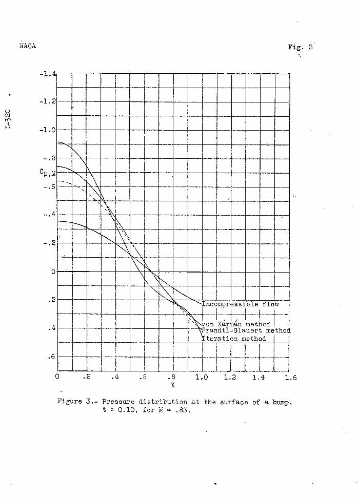
Vith the help of table V, values for C M along the profile can be easily calculated for the case t 0.0 and M 0.83. Table IX shows these values of Cp,M together with corresponding

values calculated according to the Frandtl-Glsuert rule and the von Krmn method. The Prandtl-(Glauert rule is

cp,o

Cp,M = ______

and the relation obtained by von Krirn (reference 3) is

Cr,O Cp,M ir

+

1+v4_.M2 2

Figure 3 shows the graphs of the various calculated results. It is observed that the results of the Prandtl-Glauert and the von .Ka'rmn methods differ considerably from the results of the iteration method. The reasons for these differences are that the Fraridtl-Glauert ap- proximation, though valid for Lach rumbers in the neighborhood of unity, should be utilized only for very thin shapes; whereas the

13

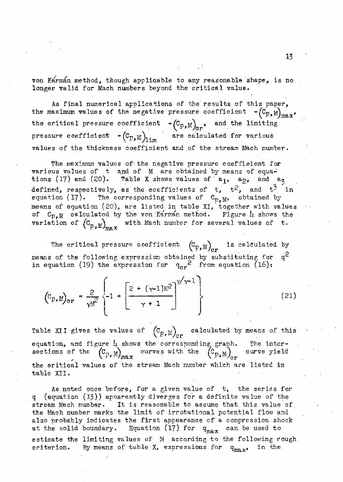
von K 'rxnnmethod, though applicable to any reasonable shape, is no longer valid for Mach numbers beyond the critical value.

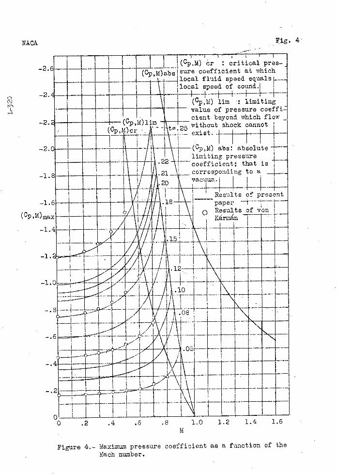
As final numerical applications of the results of this paper, the maximum values of the negative pressure coefficient

the critical pressure coefficient (Cp,Al)or and the limiting

pressure coefficient -(c1.. ' J ivr\limare calculated for various '

values of the thickness coefficient and . of the stream Mach number.

The maximum values of the negative pressure coefficient for various values of t and of M are obtained by means of equa tions (17) and (20). Table X shows values of a 1, a2, and a3

defined, respectively, as the coefficients of t, t 2, and t3 in equation (17). The corresponding values of 0nM' obtained by

means of equation (20), are listed in table XI, together with values of Cp,M calculated by the von Ka'rxnn method. Figure t shows the variation of ('CPR')

with.Mach number for several values of t. max

The critical pressure coefficient, pM) is calculated by

meaxs of the following expression obtained by substituting for q2 in equation (19) the expression for 02 from equation (16):

(

22 + (y-l)1v12

(cpM);- + + 1 -

(21)

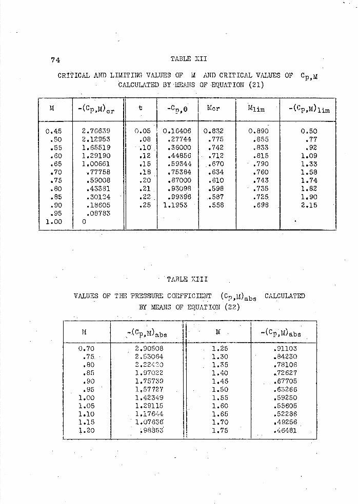
Table. XII gives, the values of (CflM' calculated by means of this

equation, and figure L. sho sections of the (c M" '¼ P "max -

the critical values of the table XII.

\ 'icr s •the corresponding granh. curves with the

stream Mach number which are

The inter-curve yield

listed in

As noted once before, for a given value of t, the series for q (equation (13)) apparently diverges for a definite value of the stream Mach number. It is reasonable to assume that this value of, the Mach number marks the limit of irrotational potential flow and also probably indicates, the first appearance of a compression shock at he solid boundary. Equation (17) forqmax can be used to

estimate the limiting values of M according to the following rough criterion. By means of table X, expressions for in the

IN

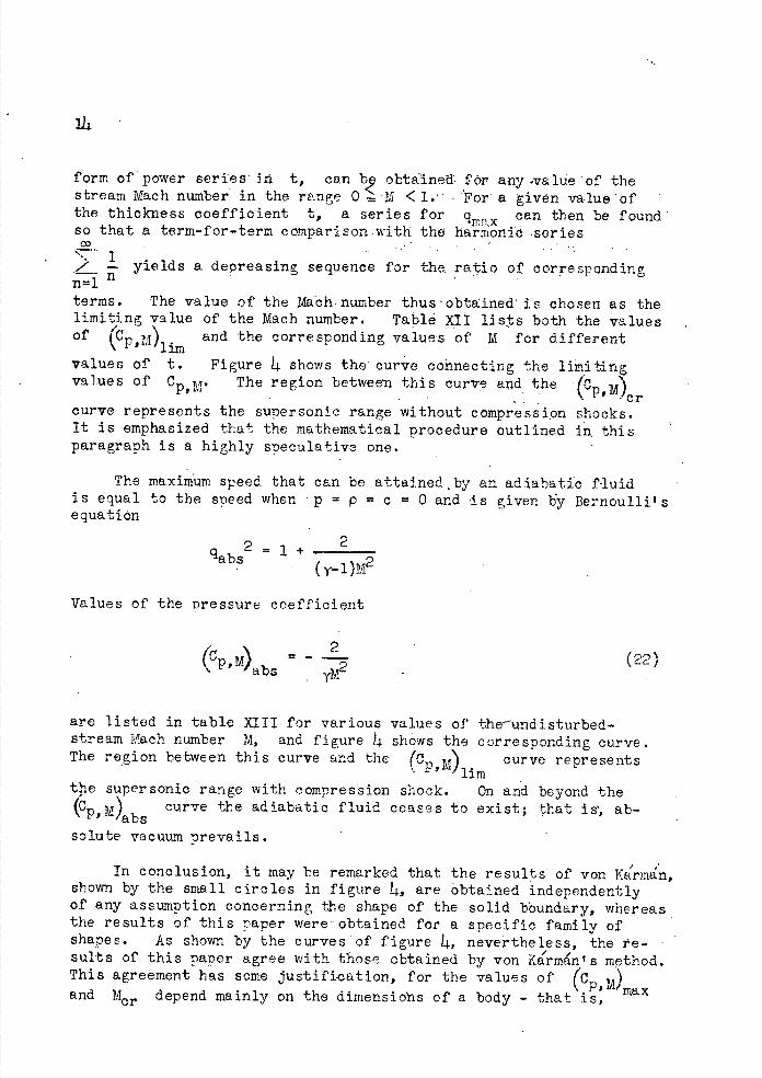
form of power series- in t, can obtained fr any .vahie of the stream Mach number in the range 0 'M <1. "Far a given value 'of the thickness coefficient t, a series for o can then be found' so that a term-for-term comparison with the hainioni' series

CO

2 ! yields a depreasing sequence for the ratio of corresponding

terms. The value of the Mach . number thus obtained' is chosen as the limiting value of the Mach number. Table XI lists both the values of(C and the corresnondjno values of M for different

\P' lim values of t. Figure 14 shows the curve cohnecting the lining values of C M . The region between this curve and the Ic M)or curve represents the supersonic range without compression shocks. It is emphasized that the mathematical procedure outlined in this paragraph is a highly speculative one.

The maximum speed that can be attaInedby an adiabatic fluid is equal to the speed when 'p = p =c = 0 and is given by Bernoulli's equation

2

(y-1 ) M

Values of the pressure coefficient

(cP ,M) - (22)

are listed in table XIII for various values of the —undisturbed-stream Mach number M, and figure 4 shows the corresponding curve. The region between this curve and the (c M) curve represents

r Urn the supersonic range with compression shock. On and beyond the

(CP,M)abscurve the adiabatic fluid ceases to exist; that is', ab-

solute vacuum prevails.

In conclusion, it may he remarked that the results of von K'rmn, shown by the small circles in figure 4, are obtained independently of any assumption concerning the shape of the solid boundary, whereas the results of this paper were--obtained for a specific family of shapes. As shown by the curves of figure 4, nevertheless, the re-sults of this paper agree with those obtained by von Karmn' s method. This agreement has some justification, for the values of (CP,M)Max and Mar depend mainly on the dimensiofls of a body - that is,

15

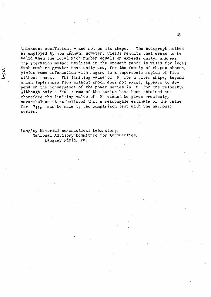
thickness coefficient - and not on its shape. The hodograph method as employed by von Ka'rman, however, yields results that cease to he valid when the local Mach number equals or exceeds unity, whereas the iteration method utilized in the present paper is valid for local

o

Mach numbers greater than unity and, for the family of shapes chosen, yields some information with regard to a supersonic region of flow without shock. The limiting value of M for a given shape, beyond which supersonic flow vdthout shock does not exist, appears to de-pend on the convergence of the power series in t for the velocity. Although only a few terms of the series have been obtained and therefore the limiting value of M cannot be given precisely, nevertheless it .is believed that a reaGonable estimate of the value for Mum can be made by the comparison test with the harmonic series.

Langley Memorial Aeronautical Laboratory, National Advisory Committee for Aeronautics,

Langley Field, Va.

d -= (1+

,)(I _ _2_) dZ'

(A-2)

16

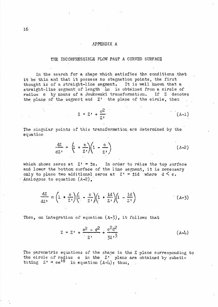
APPENDIX A

THE INCOMPRESSIBLE FLOW PAST A CURVED SURFACE

In the search for a shape which satisfies the conditions that it he thin and that it possess no stagnation points, the first thought is of a straight-line segment. It is well known that a straight-line segment of length 4c is obtained from a circle of radius c by means of a Joukowski transformation. If Z denotes the planp of the segment and Z' the plane of the circle, then

t +ZI (A-i)

The singular points of this transformation are determined by the equation

which shows zeros at Z' 2. ±c. In order to raise the top surface and lower the bottom surface of the line segment, it is necessary only to place two additional zeros at Z' ±id where d < c. Analogous to equation (A-2),

dZ / c' c id \/ id\ + 1 1 +-(l -

dZ' \ -(A-3)

Then, on integration of equation (A-3), it follows that

Zzt02 - d2 c2d2

+3Z

(A-Li.)

The parametric equations of the shape in the Z plane corresponding to the circle of radius c in the Z' plane are obtaind by substi-tuting Z = ce 9 in equation (A-Li.); thus,

17

X 2c cos 9 -

( 3 cos 9 - cos 38) 1 (A-5) d2 Y — (3 sin O-sin38) 3c

The family of shapes given by equations ( A-5) includes, on one hand, the straight-line segment with d 0 and, on the other hand, a shape having four cusps srrnetrioa]ly placed with respect to the co-ordinate axes with d c. For 0< d <c, the slope dY/dX is zero for e o, 1r/2, and Tr. The shape thushas ouss at

/d2 X ±2c(1 - - ), Y 0, and the maximum and minimum points are

.\ 3c/ •Ld2 Ld2 at X 0, Y - - and X 0, Y - , respectively.. 3c 3c

The complex potential for a circular cylinder of radius c, fixed in a stream of uniform velocity U in, the positive direc tion of the real axis, is given by

/ F = U (Z' +

C2)(A-6)

The complex velocity past the corresponding shape in the Z plane is

dF dFdZ' U - iv - = - -

dZ dZ' dZ

or

q2 U2 = 2 2 2 dF d!: dZ' dZ' __. dZ' dZ V dZ dZ

By means of equations (A-Li.) and (A-6), it follows that

18

(

1)( c2'\

-- l-Ii.

q2 T,,2 -

(1- d2 c2d2\ I' - 2 - 2 C2d2\

Z 12 - - z / - \

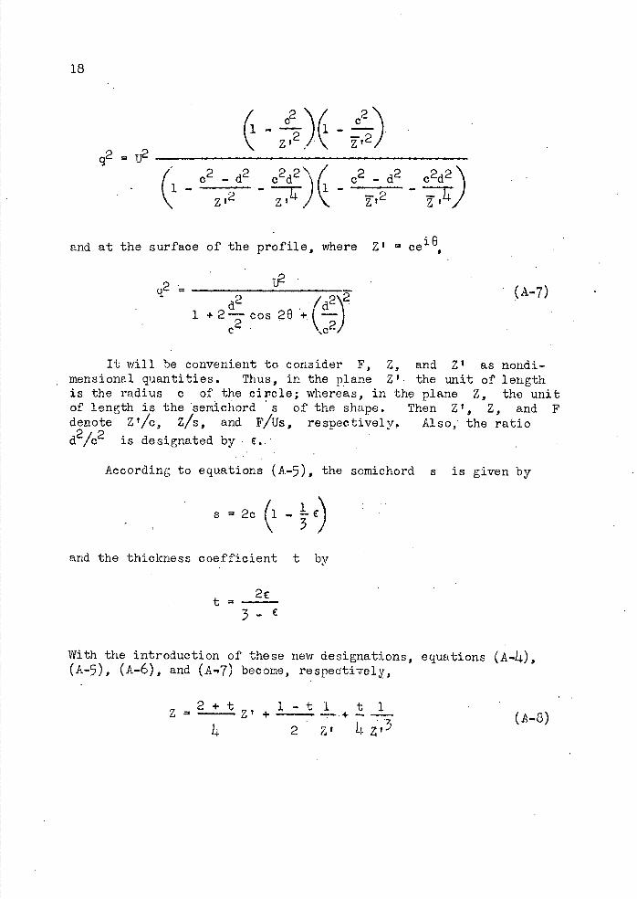
and at the surface of the profile, where Z' = ce ie

2 ______ ( A-7)

1 +2— cos 29 +1 — C? . 'c 2)

It will be convenient to consider F, Z, mensional quantities. Thus, in the plane Z' is the radius c of the circle; whereas, in t of length is the semi.chord s of the shape. denote Z'/c, Z/s, and F/Us, respectively.

d 2/c2 is designated by

and Z' as nondi-the unit of length

he plane Z, the unit Then Z', Z, and F

Also, the ratio

According to equations (A-5), the semichord s is given by

s2c(1_E)

and the thickness coefficient t by

2€ t= 3- €

With the introduction of these new designations, equations (A-4), (A-5), (A-6), and (A-7) become, respectively,

2^t 1-ti t Z Z + -- + — — (A-3)

2 Z'

19

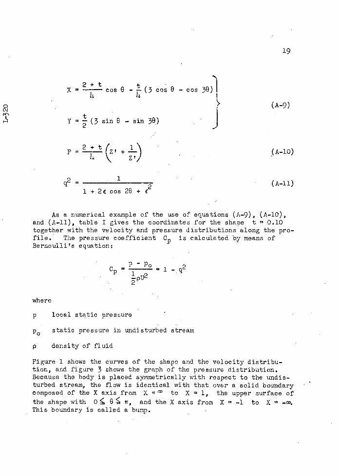
2+ t = cos 9 - (3 cos 8 - cos 38)1

0 (A-9)

(3 sin 8 - sin 39) J

F -fr- (zt + S(A-b)

ZI)

q2 =

1 0

2(A-li)

1 + 2c cos 28 + C

As a numerical example of the use of equations (A-9) ., (A-b), and (A-li), table I gives the coordinates for the sha pe t 0.10 together with the velocity and pressure distributions along the pro-file. The pressure coefficient C is calculated by means of Bernoulli's equation:

C -pU2

where

p local static pressure

POstatic pressure in undisturbed stream

P density of fluid

Figure 1 shows the curves of the shape and the velocity distribu-tion, and figure 3 shows the graph of the pressure distribution. Because the body is placed symmetrically with respect to the undis-turbed stream, the flow is identical with that over a solid boundary composed of the X axis from X to X 1, the upper surface of

the shape with 0 9 rr, and the X axis from X -1 to X This boundary is called a bump.

20

APPENDIX B

THE COMPRESSIBLE FLOW PAST A BUMP

0 and Y in positive, integral powers of the thickness parameter t Before proceeding with the iteration process, developments for

must be obtained. From equation (A-8),

if I .1

t '.- -' tS-.i)

-1, '\ z')

and from equation. (A-10),

Z _ — (Z ? +—) 2 \ Z'j1,

F (B-2) 2Tf'1_L\2

" z?J

— zti.J.IBy means of a Taylor expansion in the neighborhood of t 0, it is possible to express F as a power series in t in which the coef-ficints are functions of Z. Thus, according to equation (B-i), t0 when

Z -IZ' + - 2\ Z',

or

zt = z + \/Z- •i

where the positive sign is talk-en with the radical because the points at infinity of the Z and Z' planes must correspond. Now

LF F (F)t0 + t (\) + •

t=O

21

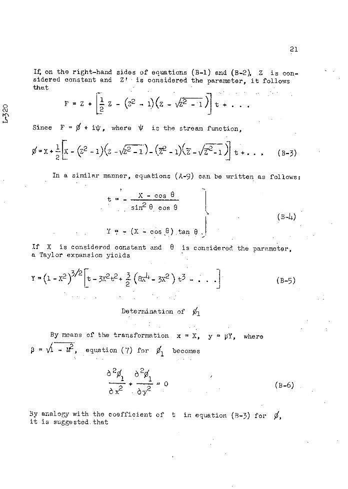
on the right-hand sides of equations (B-i) and (B-2), Z is cOfl-sidered constant and Z' is considered the parameter, it follows that

0

F z +

z - (z2 - 1) (z - Jz2 -1 t Since F 0 + ij, whore '4i is the stream function,

=: X +.LF (B-3)

In a similar manner, equations (A-9) can be written as follows:

- C os9

sin2 9 cos 9(B-Li.)

Y-(X-oosQ)tan9

If X is considered constant and 9 is considered the parameter, a Taylor ex pansion yields

Y= (1 - x2 )3/2

Ft - 3X2 t2 + (aX - 3X2 ) t3 - (B-5)

Determination of $1

By means of the transformation x = X, y 3Y, where

P = vl - iv, equation (7) for becomes

à 2 a 20 /(B-6)

By analogy with the coefficient of t in equation (B-) for 0, it is suggested, that

22

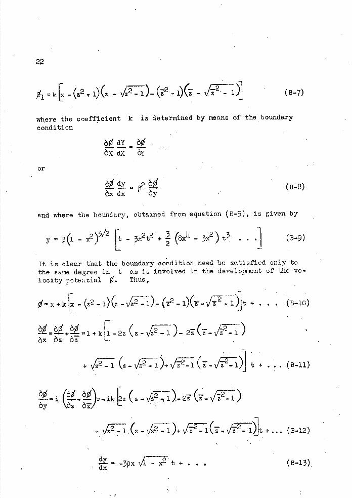
Ø(z21)(z/)(1)( l)] (B-7)

where the coefficient k is determined by means of the boundary

condition

ôXdX ô

or

ax dx ày (B-8)

and where the boundary, obtained from equation ( B-5), is given by

( -

)3/2 [ 3x2 b2 + (x - 3x2 ) t . .

(B9)

It is clear that the boundary condition need he satisfied only to the same degree in 1 as is involved in the development of the ve-

locity poteitia1 0'. Thus,

+.... (-io)

=+l+1-2z (-)- 2&-l) àz àz -.

... ii)

2z ( z - Vz ),27( 6^ . i. (6^ - ày àr -

rz^^-1 (z - VZT - 1 )+ V^Z^- i + (B-12)

-3x v'i - 2 t + , • • (B-13),

23

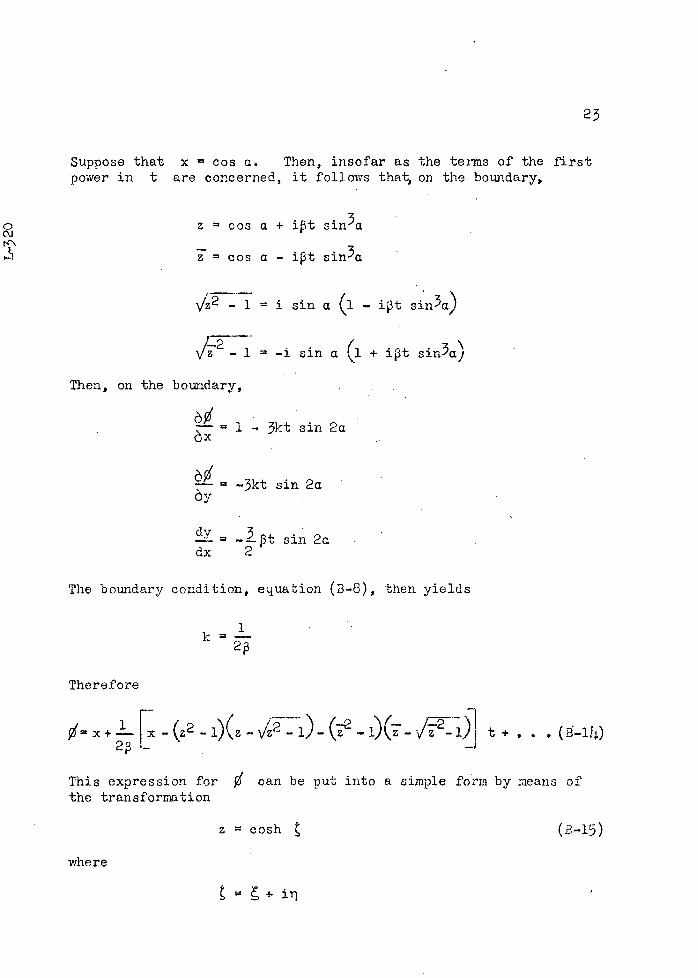
Suppose that x cos a. Then, insofar as the terms of the first power in t are concerned, it follows that, on the boundary,

o z = cos a + it sin3a

z = cos a - i3t sin3a

V'Zl I sin a (i - i3t sin3a)

1-2 ( VZ - 1 -i sin a \l + i3t sin-'a)

Then, on the boundary,

1 - 3kt sin 2a

6^ = -3kt sin 2a

dv 3 = -_13t sin 2a

dx 2

The boundary condition, equation (3-8), then yields

1 k

2

Therefore

(-'1)

This expression for 0 can he put into a simple form by means of the transformation

z cosh (B-l5)

where

21

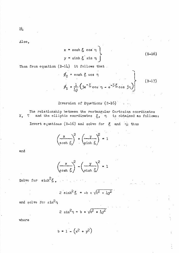
Also,

x cosh cos(B-16)

y sinh sin

Then from equation (B-u.) it follows that

00 cosh coi11

(B-17)

01 =In -(3ecos n - ecos 31)1

Inversion of Equations-(B-16)

The relationship between the rectangular Cartesian coordinates X, and the elliptic coordinates , . is obtained as follows:

Invert equations (B-16) and solve for and r1 ; thus

(c osh

x+

;, \sinh

and

2

(siah çosh )

. 2 Solve for sixth ,,

2 sinh2 , = -b + V+ and solve for sin2r

2 sin2i b +

where

b i - (x2 + 2)

25

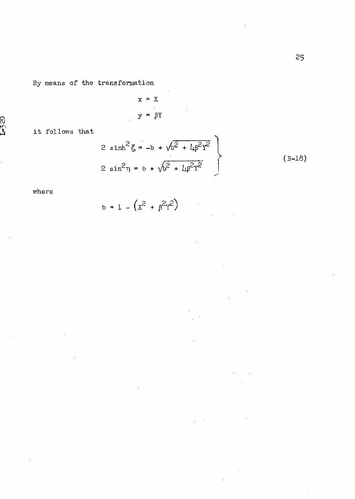
By means of the transformation

xX

Y=

it follows that

2 sinh2 -b ++ 1 (B-la)

2 sin2ii = b + /

_

+ L2Y2

where

/' 2 b = 1 - +

26

APPENDIX C

DETERMINATION OF 0'2

The differential equation (8) for ø'2 in terms of the co-ordinates x and y becomes

L2 62

p2-

L2- + ; 6 1 - (Y+'),

I a% a2ø1 + 6 X y2 2 ax

21 + (y-1)3

a2 2 + 23 _

ax 6 Y ày

By means of the symbolic relations

ax àz àz

a 2 a2 —=—+2 ax2 àz2

a ./a a -=11-.- ày àz a? )

2 2 2 a a

6y2 62 àzà? oz

a2 .(a a2

(C-i)

27

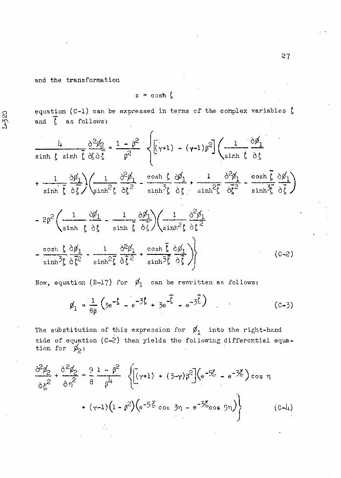
and the transformation

z = cosh

a equation (c-i) can be expressed in terms of the complex variables

and as follows-:

* 60o 1 - 2. 1I +1) - (yl)2] (sin h_

i

sinh sinh p2

1-1 Pi i - cosh 1 à2Ø'1 - cosh %l"\ +

sinh ÔJc1flh2 2 sinh3 6 t:S

inj,2E 2 sinh à)

2( 1 _"\(_L -i

sinh à sinh à)sin22

- cosh 1

62Ø cosh

sith3 62 - sinh2 2 + sinh à(c-2)

•1

Now, equation (B-17) for 01 can be rewritten as follows:

01 (3e - e + 3e - e 3 ) ( c-3)

The substitution of this expression for into the right-hand

side of equation (C_2) then yields the following differential equa-tion for 02:

+2022

+ (3Y)2](e5 - e3)cos 8

+ (y_l)(1_p2)(e5cos q - ecos (c-a)

28

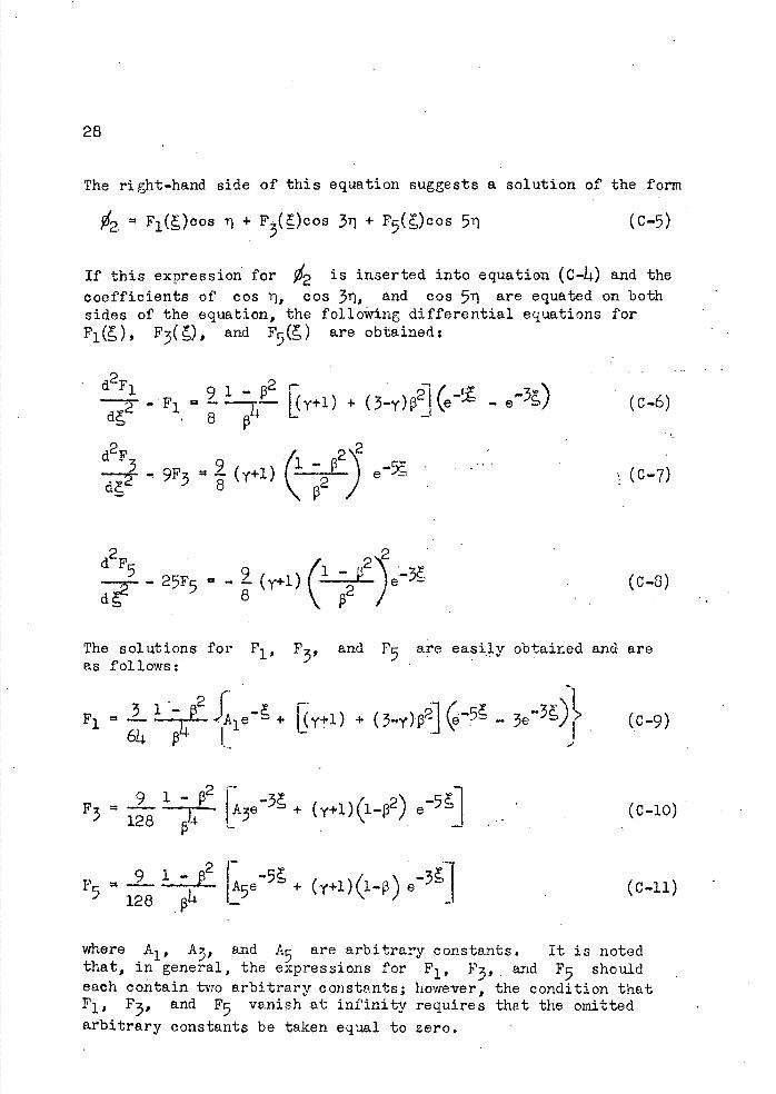
The right-hand side of this equation suggests a solution of the form

X,,, , F1 (,)cos + F3()cos 3 + F5 (,)cos 5i (C-5)

If this expression for Ø2 is inserted into equation (c-4) and the

coefficients of cos 1, cos 3i, and cos 5i are equated on both sides of the equation, the following differential equations for F1(), F3(), and F5() are obtained:

:

- F1 +l)+(3y)2l (e -

9F3 (y+l) ;2) e-5-r'; (c-7)

25F5 - (y+l) ( 2)e (c-a) dg 8

The solutions for F 1 . F3, and F5 are easily obtained and are as follows:

F12 1 + + ( 3 )p2] -s - 3e3)

F3 [e3 + (+1)(ip2)

F ZX1 2

+ (y+l)(lp) e -3 128

(c -9)

(c-b)

(c-il)

where A1 , A3, and A5 are arbitrary constants. It is noted that, in general, the expressions for F 1 , F3 1 and F5 should each contain tvro arbitrary constants however, the condition that F1 , F3, and F5 vanish at infinity requires that the omitted arbitrary constants be taken equal to zero.

El

29

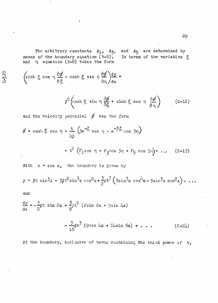
The arbitrary constants Al, A 3 , and A5 are determined by means of the boundary equation (B-8). In terms of the variables and equation (B—B) takes the form

0 C" ^dy

(sini cos Tj coshJdx

2 sin il + sinh cos -q (0-12) . ( 611

and the velocity potential Ø has the form

cosh cos rt

+ - (3e cos n -

3n) e cos

+ t2 ( i cos + F3cos 3i + F5 cos 5)+ .. (0-13)

With x cos a, the boundary is given by

y = 31 s 4 n3 - 33t2 sin 3a cos2a+t3 (8sin3a cost a_3sin3a cos2ci)_

and

dL

sin 2a + t2 (2sin 2a + 5sin La) dx 2 6

- _-_t3 (9sin L.a + lLi.sin 6a) + . . . (C—lL.)

At the boundary, inclusive of terms containing the third power of t,

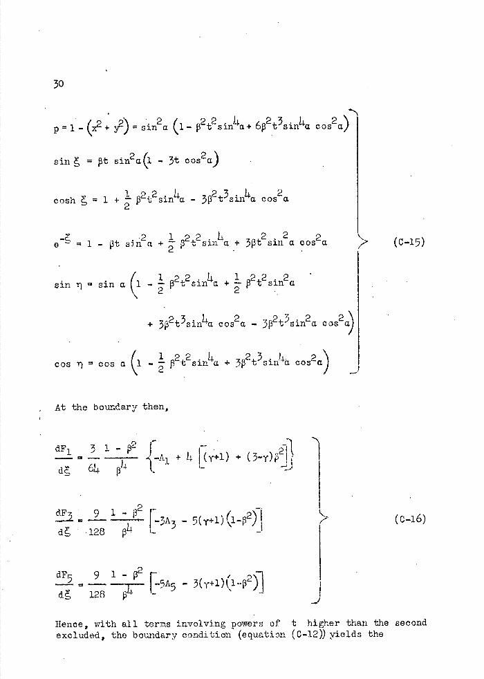
pi_(x2+ y2)=sin2a (i_ p2t2 s in4a + 6 2t3sin4a cos2a)

sin t sincL(1 - 3t cos 2a)

t sin a cos 2

a cosh , 1 + - 2t2sinL!4•a - 332 3 . 14 2

- 2 12214 2 2 e 1 - 3t sin a + t sin a, + 3t sin a cost a ,> (C -15)

(l 1 - - t sin a + - 3 tsinTh 1 22.14 1 22 2 2 2

+ 30 2t3sin4a cos2a 3 32t3sin2 a cos2a)

1 22.14 cos r cos a (i - . 3 •t sin a + 23.14

At the boundary then,

dF1 3 1 _2 —: 21i - -Al. + 14 1 (y+1) + (3-y)p

d, 614 P I-

d 128 F3A3 - 5(y^1)(1 2)1 (c -16)

- I

dF5 9 i - 2 1--5A5 -

Hence, with all terms involving powers of t higher than the second excluded, the boundary condition (equation (C-12)) yields the

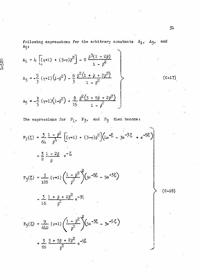
31

following expressions for the arbitrary constants A l ,-A3, and A5:

3(i - 2) a Aly+1)+(3_y)2]_8 i_2 ('J

A3 = - (Y+1) 2) - p2l+ 2)

3 i-.2(c-17)

8 p2(3 + 53 + 22) A5 -

(+i)(i 2) +-

The expressions for F1 , F3, and F5 then become:

3 1 - - + - 3. 3 -5) 64 p

0 +0

_l -23

8

F () = (Y#1) '

- 5e3) 128

(c-18)

- i 1 + + 2p e3 16 p2

F5() = (y+1) (i ;2)(5e - 3e) 640

80

32

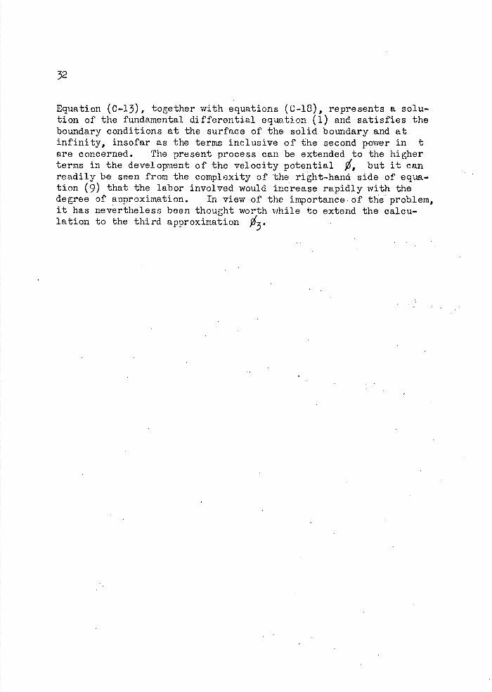
Equation (C-13), together with equations (C-18), represents a solu-tion of the fundamental differential equation (1) and satisfies the boundary conditions at the surface of the solid boundary and at infinity, insofar as the terms inclusive of the second power in t are concerned. The present process can be extended to the higher terms in the development of the velocity potential ', but it can readily be seen from the complexity of the right-hand side of equa-tion (9) that the labor involved would increase rapidly with the degree of aproximation. In view of the importance-of the problem, it has nevertheless been thought worth while to extend the calcu-lation to the third approximation Ø•

33

APPENDIX D

DETERMINATION OF 0

The differential equation (9) for in termof the' cmpiex variableE z and z can be written as follows:

y+l)(ip2 )2 + 21 (̂ j .. + + 3z'F 2 F

+ ( i+1 ) (l_ +

+y+l) (i )+ 2 t(i + ) (ø z + 2 ) + + ) ( z +

+ 2[(+l)(l+2) - 22j(Øl + 1l)02z

2[(Xjz2_XlZ%j7 _^JEZ)+ø2!l%1ff)

X2 ilz + - -(p-i)

where, for example,

p3

3zz àzàz

Again, complex variables , and are introduced in place of z and z by means of the transformation

zcosh

34

According to equation (c-3),

- + 3e- e 3) (03)

Consider the term

- L(y+1)(12) + + + 2\ lz I

+ ( y+1 )(1 - 314X 'i + 232(Øj - 0'ir)('iz2 _i2)

Now

d - 3 -2

e2 0 --- - lzz23 sinh

and

0 2 + 2 9 e cos - 82

ø'1z2 01z-9j esin Lp

e 162

3 e cos 311 - e 3 cos T 0lzz 213 sinh sixth -

Iji;j

ø'lzz - 01 11e- ^ sin 31- e 3 sin Ti

2P sinh sinh

0 CM

It follows then that

T 1 sinh t sinh

k+l)(l2)2 +82 ] e - 2(+1) (1)e 7 }cos 1

+(y+i)l-e 5 _r+l)(l 2 + cos

- ( y+l ) (l 2)2e 7cos 51 +(+1)(1_2)2o_5 cos 71 (D-2)

In the handling of the terms on the right-haid side of equa-tion (D-1) that contain the derivatives of 02, it is convenient

to separate 02 into two prts: namely, 02', which is a function

of plus a function of t, and 02", which is a function of

and t. Thus, if the variables t and t are introduced into the expression for X20 it follows easily that

X2 '=A6e- t - +

34 - e 3 )+Be 3 - 3e + 5e-31 - 3e5)

02" C(Le 3e- t-2 (D-3)

+ D(-8e + e +ec - 8e+ e" +e') J

36

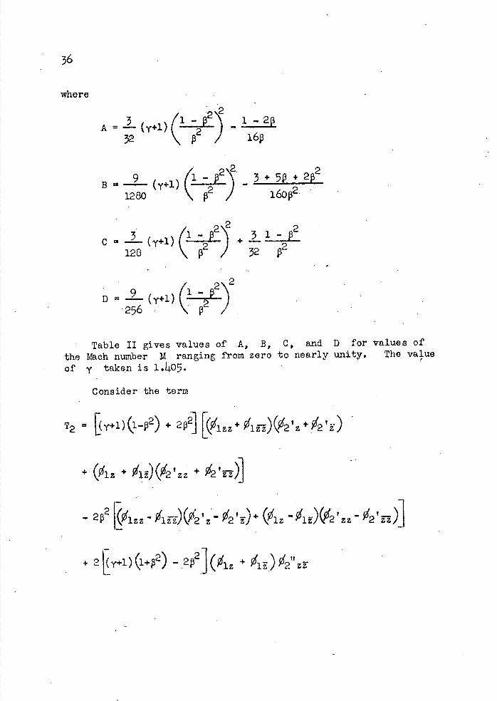
where

A =1(Y+l)(1t25 _l —2

32 \ 16p

B((1\_3+52P

+l)

i6op2 1280 2 )

C (+1)- 1 -

128 2 )

+

32

= (y+1)4P)

256

• Table II gives values of A, B, C, and D for values of the Mach number M ranging from zero to nearly unity. The value of y taken is 1.405.

Consider the term

= [(+1)(1_p2) + 2P2]

+ + ø1)(ø'2'zz +

- 2p 2 [^^l Z z /1 i V2 z- /2 ' 0 + V1 z ^l 2) V2 7 z X2 Z—z

+ 2(Y+1)(1+02) - 2p2](Øl +

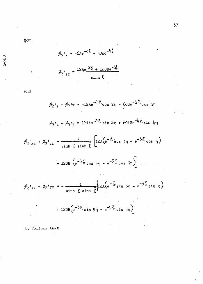
"ow

- 3OBo -6Ae 0 '2z cJ

12Ae_2 + 12OB& '2 ' zz

sinh

and

ø'2'z + ø2'i -12Aecos 2r - 60o'oos Lr

- 12iAe' sin ?r + 6OiBe'rin 1rn 2z 2z

02 ' zz + --oos - eco6

sinh t stnh -

+ 120B (e 3 cos 511 - 3'i)} e -cos

zz - 2 zz- 2A(esin 3r - e-39 sin 11)

si.nh t sinh gl '.

+ 12OB(e 3 sin 5ij - sin

37

It follows that

38

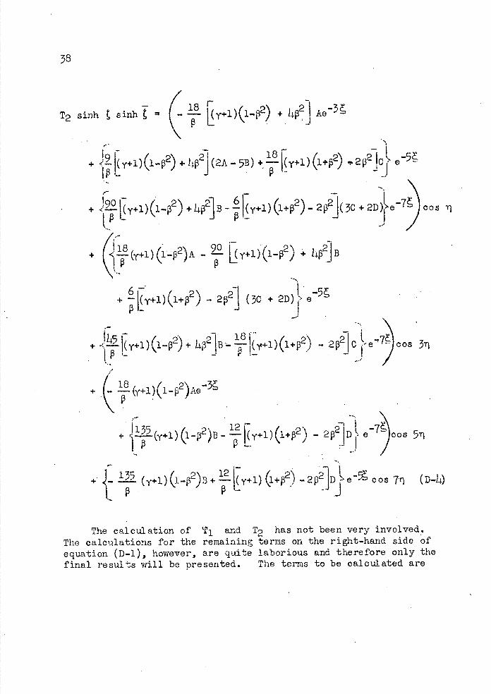
T2 sinh sink = ! y+1)(l_2) + 1 Ae3

+ i(y+l)(l- p2) +ii(2A-5B) +(y+l)(l+2) ,2p2!c

+ 20y+1)(l2)+2]B

+ (y+l) (l- 2)A - 20- L( y+l) (1- 2) + B

6 ^ - 2j (3c

+ +l)(l2)+4P2tB.!!+1)(1+2)

+ 8(y+l)(12)Ae3

+ 15(Y+1)(lp2)B - 1(y+l)(l+2) - 2 2 D e Cos

(y+1)(l2)3+!I(y+1)(1+2) 2P2jDjecos 7 (D-)

The calculation of Tl and T2 has not been very involved. The calculations for the remaining terms on the right-hand side of equation (D-l), however, are quite laborious and therefore only the final results will be presented. The terms to be calculated are

+ 2D)

2il- 3i

L

39

0 c'J

+

+

I

+t.)

IGL

I

. ('J

'a.' )•

c'J

+ .. +

('J Co.

I C'JCo.

'S# r1 +

LJc'.I

(

+

(I

It II It

H

- E-4

U H H

to

to FPC)0

941)

N-

V N-

CC.

0) N-

.0

C)

N

I

I

0) -

Jl I Lc\

Lf\

C.)

-Ji L\

I

C)

+

N- C.) KN

co

r('% )&fl KN

-

ri

I0)

+ ('J

+ F-'

9&I) + co)1J

IC)

tjj C).

co

0 C) C)

+

I N-- I (\I

tO C) (I)C) I

C)

0 (\J

I ()

10J

to .--- :-• + to Ci IoJ

Co.0 C)

0) CJ

+

,u) 0

._Q.'to

•0

&J)

U)

E c'i N-

0)Co.

II

C.)N-

.Q)

to

id 4)U-'

C) U) C)

-S.-4 +

Lldj

.

I

+

- -P

>-

LJ

C.) Lr\ I CU

o+

a) Co.

to

II r-e I

C) IF-,.

0, N

I

a) Go

+

•r-I Cl)

•rl U) I

tJ)001

+ + a) ..4

co a)

H H

240

fZ

a

R 1%

0rA

-.----C) 1

0!

'-4 oIc'j

P Ia P .-4 1r4

(0 0 vi

LC\CO

I IC')

N-N-

N-I Ic'.

+ ,c'J

+ Ci) I a) co

+a)

u-\Lc'. .-4

a) Ic'

Ia)

94_n I I I r4 a)

a,94_n Ic'.

9j) Ic'. I

+ +

F4\ I I a) + N- '0

Cd I

I kJ)

-;f + Pr:: --1

.

&fl a)

ii 0 0

a)

-,•4

r

+

94fl + )4J) +I L_9J

Ci)

co

co

0I

a) \ ik-i

tocj

+I

a) t

a) F4\ I CO to

fj1 Ci) CZ)

01 0 C)

0 -zt . P + I C) '-.....--' (0 I

Cd--.

1-.L

Cd +

Lf\

+ C) U) Cd 17 If'.

a)P

,'tf)

+C) /

f— 0 C)

I

'0

Cl) 0 C)

+

94_n

CO 0

Ia) -

lCdC') 0 a)

.-4

+a)

Ic'. Ic' ,- I

M

C)

M. Cd

° '" xJ)

+ Go\••# + a) N-

I rC'.+

+ O' 14_n to

I

94_n +

a) -

Cd Ia)

Cd-

a) I 94J) C1

a) CQ &fl

If'.+ '-

J Q Ir-4

s-...-'

+

N-

)

U4J)

, •ri +

1i

C) a)P Lc' 94_n

- .-4

ICi)

N- I r-i Cd Cd Cd

C\j + \ (I) C. Cd

Ia) +

'-0 kfl

o 0

co0 C)

l'—

1'c'I(X)..J)

If'.I + Cd

+Cd

II

a) CO N-

I.J) II

Ia)

ri'.rC,

I

Cd I

-

a)

+

-zt -I-1 + stJ)

'-.zi- .—.

+

J) +

r4 U)

a) _- I

.r4 (0 r1

Cl)

\ IC)

+ -

94Ji

r1 +

Cda) Ic' L_J

C:::: P ca.

ON---'

'' \0 Jccx.. Cd

+ + + + + + + . I

Cl)'-3

(I)

_z

14

0

co 0 C.,

a)

+

a)

a)

+

C-)

Co

co

U)

Co1

0I..-'

0 C)

I U)

Lf

9&I)

-zt

+ a)

+

a)

4f1 I__l —+ I

I0J -+ c'i.H

kn KN

U) 0 0 +

'

'.j_-J

4J)

t? )

a) KN

I

a)

cc

(-'J+

N-+ + .- (\J

+

co 0

(I) o

C) r4 + I

C) kfl a)

a) .-zr +

+ a) 9_f)

W t'C\ r-c- + a)

4J)

to &J)

G) fl a) 'tJ1

N- I L_ I Cl) 0

+ a) C)

9J)I U)

9J) '-0

I C C)

+I

a)94J)

-zrU)

4J) ¶4_fl

I .-Ic\J

I

C) s4.j)

C)

to C)

'—, '—, —ztco

+ + I +

Cl) U)U) 0

0 0 C.) C) C)

9tfl

- N-ON

I I C)

a.)

-1

C) N-

N--

+ ++

Rf-C\

I I . -c\ I C)

N-a) r1 U)

CI) Lr\

0

C.)

+

+ &J) +

4J r-4 4.j) - ON I .-I

C)a) -4

IC)

N-Lc\ a)

lç\

+ +'-4

+

+

U)

o

I ,-4a-

I

'-4

r1N-

a) trN a)

(I) N-

o.-C r-1

U\\

+

+ + +

M '4i tJ)

CI) -1 I I -4-) tf- a) a) C)

- N-

+

+ + +

.0 J) fl CI) N.

ILc-

IN-

I a)

rC)

ua) -

N-N-

Cd C) c:i + + +

II '4M fl —1 i-41 U

I IL

I a)

L

a)

r

a) N-

+ + + + ci

CTI1bI'o

142

T

C) KIN

. +r4

C)

+ C)

J) LN

I N- I

+C).

r1CU I N-

+ C) o 94_f)

cr C

4j) .

CU I C) CU

+ . r-1 IC) CU

C) CU

1

9tfl+

KN

r1

I

C) +

,_-..

945) + .-4 94.1) .1 CU CI) re

I

C])

+

C])I

. 0)

•CI) 0 CU

C) +

In r t.C\

C)J) I

r4 I

N- I

C]) CU

____ r4 c%J '-I

r4 9thC)

r1 +

9fl

I

Cs I +

+ 94.1) . r-i 94J)

v-i I

UN+

C) 0

9f) If\

r-1 I C)

C)

N- I

CU

+v-I

IC).

I(I)

('J

C)

+

•I . C)

CU

+

L_aJCI) N- 94j)

r-10 CU

s—' L2J

N-+

Mi)

Iv--C

I CI) r-(.C) (\J

CD.Q

C) (U 00.

.

C)

Ci

+ -'kA

CU

C.' -v—I rl

+C)

CU

+CI)

+ I ++

KN I tC. r1 N- \OI, 9f) .

CU f C.) N-

--'

CU

.

CI)

.

I I- mCo.CU II -

r4I CU CU HI CU CU CU

+ + •+ +. + + . + +

0) C4

co

4,

c-I 0

i. C)

4'

C)

•r-4

C) I-.

C)-4

43

I-I 0

4.-I

(D

4)

4-4 0

0 -H 4)

'-4 0

cs

U) 4)

co C)

U)

0

-P

C)

4-4 0

C) Id --4

U)

Cd

•0

4.,

C)

o r-1 (\J - ,-4 _-4 _-4 ,-1

I RO I I I I --4

(1) -P - .-, .-o o...----.--.---

C) )4M 4J) 4-4 N-- Or4 4

I I U)-rl C) C) R

4-3 4-" N-

N- C) C) e-4 + •H-

0 C) + +

0J 4-44-I 4-i -H

U) C) t4 0 r4 o o I C) o r-4 C) N-

N- C) -H C) - N**, - + 43

+ C\J r-4 . 4 I +

+ -4 dc- r4

—4 I

-'C) . C) C) N-

+ I-P I + C)

ri N- —4 -i -Z

C) ,-4 U) 0-P + J) 0 •H d + 0 -P r-e '-4

as 04 r-A QI

0-• —4 0) a) N-

C.— C) C)C) C) 0 4 + —4

0 as -H + 4)

__'\.J) +

+S iJ)

-H 0, D I N-C)

C) I to C) C) . I. (1) 0 4) 1r., C) N- N-C) CY' d .-4

C) C) N- + + co .14 + ti)

oN- . + LS\ •ri + 0 -P0 I N-

CC 'N U\ (D C) l + -H4-40 I If\ C)

0 a) . N- Lf. N- N-

WN Lr\ ++

U) tja) + 0 9if) C) I-. C

0 • I C) 1 I C) C)

4)0 Ui N--

0 -4 U - 0

—_, -ri - + U) 1f\

C)

0

CO J CC 00 (NI

$ I OJ aL_

0 r-c- r41 U) •L)

&i) CO • - KN 0 0 -H - 0 0 u C'-

1 C ,-4 (J's (N zt 0 I I

C) U) 9-i

0r,f)

9g' Lr-I

I , 00 (N

tfl Ln r

ci)

+

9J) NN

Ia)

Cu

p4-n (-4

Ici)

+

tfl.

ci)

Q) Cu

+

s4J)

a)

Cd

+

'th 0'

Ia)

+

kn (s-9$

r

Cd

+

I a)

+

LJ

Cd

+

a)

U-'

Ia)

+

.-1

ci) Cu

a) Cu

+

ci)

Cu

+

CH

Cd

11

Ea

r

an

a)

a) rI Cu +

a) Cu

ca.

C-+

Cu

C-+

Cu

cli

+1

a)

+

p4-n

Lr\ -4

9&f) rc-

ci) 0 Cu

+

r

Q) N-Cu

+ ,t.

--4

L2J Cu r-I

+

a)

kn WN

Oj

ON

+

9J1 N-

Cu

+

a) +

I ci) r

a) Cd +

-4 I

ci)

C--

+

L

L_J Cu

Cu.Cu

I c.

r4

+

a) '-I -4 +

a) 0 Cu

ME

a) a" +

ci) C-

94fl L

a) Cu

+

,J) Nj

ci)

Cu

+

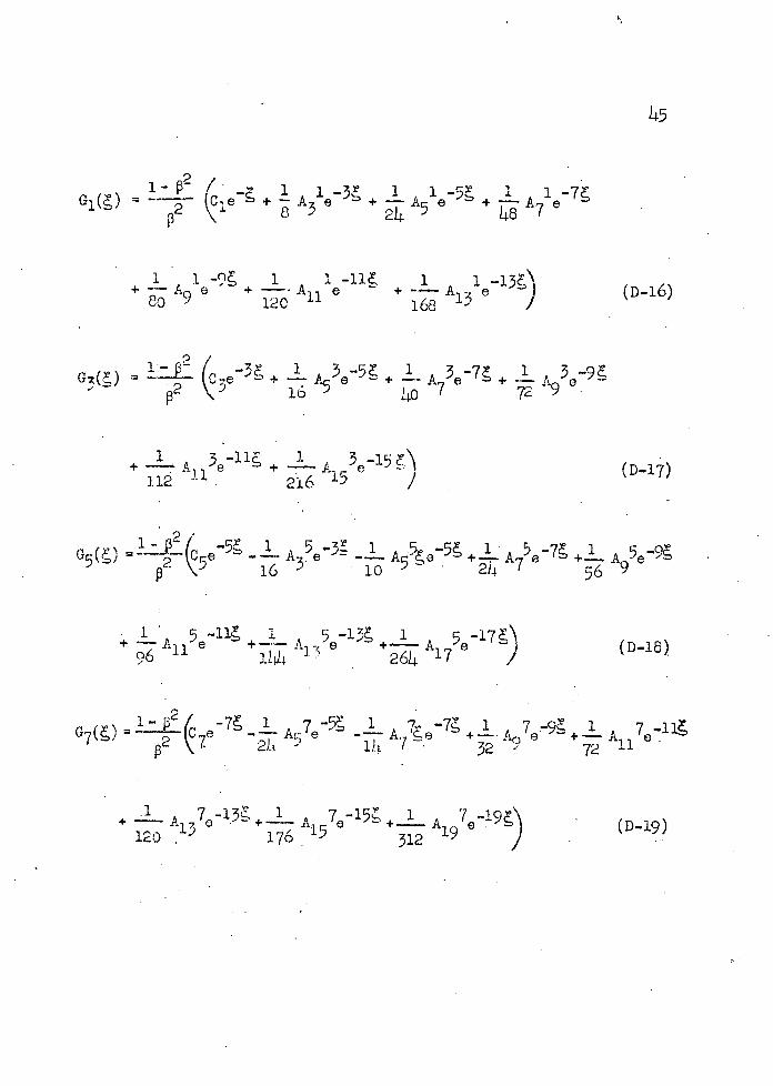
P2%/ I 1-7 -"- CeS + ! A31e 3 + -i-- A51e + - A7 e

24 48

1 1 -9 1 1 -11

+—A0 e +120

e + -- A13 e)

(D-16)

G) = (e3 + - + A + -i lb 729

Al I

3e h1 + 1 A 3e15 (D-17) 112 216 15 J

G5() f(5eS - A3 8 - Ae5 +

A75e + A95e9

+

96°A3 e 1

Ai75e17) (D-18)

G7() = 1(c77

+

+ A1 -13, ^_.L A 7 +J A1 . 7e_19 ) (D-19) 120 176 312

46

Cd I

Cd

0 Cd

+R N-

iJI U)co 0

0 0 C)

C)

C) 0N--

rI ° r4 C) + C) CH.

I 94_I)

f) tC\1

to 0

Lr'

a) C) 4-' 4)

C) F'C\ 0

C)

+ r1 + kfl Lf

I 4J)

Cd r-1 U) a)

Q)CO it

C)

I0

J)-s

.00 C)

I ,-41C0 ''i- N- 0 c-4

\-'P

9&f} ++ Cd

'-PN-

co 0

WNfl I

a) co0

'-0 I(I) 'IS..

+ 0

C)J)

r-C

94_I) (\J

a)

r4(\0,-i _1

94f)P

N-a)

0) I CO I co

+ I

94-i)94J)

•'-00) -P

P,0 0

P U

P

I___ _____ -Zr I

I 0) 4-' 94J) co

co 0

0) r-4CO

+0

a)

0

C) C)

+ + '0

I-P •r-1

I+

C)

- I(D 0

0P

P + r-IIC'J C) -4JO U) I P >-

+ \IcoC) I>

0 C) U)

1

IC\i

K-N 941) + 94-i) C)0 C) U) 0

+Cd Cd I

a)

0 0

+

Cd . C) :

CQ

C

0+ 941)

Cd +C4-4 co- C\J

I9ij) 0 +

to C U)

C)J I a:)-IC'J

a)j_QJ 'JCd U) P

C) r4

L ' tI C)

. 0 0 I Cd Cd 04 C) -P

II + + + C) j) + +

-'S 0)

co

E-4 0

0

+

s::.

)47

-S • '-S (J u_• (\J t) s-I 0

o 3 C.)

4-' '-5'-P t'C\ -H

o 9i.j)

Cu$c)

0 i-I 4-' CH CO C)

C)

00

-O9.4

0 + 9.. 0 '-4

s-i 94J0

o co 4.) '•&.Ic;- .0

4-i 1C) .04' ,oI'O a)

G)

N'-4 4.)o

CO -H

0

C)-P

4) 0-'. oC'j 94_f)

-H

o . S

4.' -4 C) I - -

C)4)

C) 4.'

J)

Cu -P

+ CO I

,- I

(1)

-P0

• -H+

4'

C) C) ai Po

04-'

Co. a) Cu

s- J_zt -H C) C)4

p

C.) r-4 (0 + + -P -HC)C)

'-.- ,iD -H

I 94_f)CO

94_i)'.0

ICo

I .-P 0

-H-' 0 14 CH

oCu

C) C) f

C)

-P

C) -H Co1+'

0-H

•1 I I Co CO4'O. Ey'

a) Cu

.

I al

'

C)

°-'Cu oa

I 4-' .-­4 ca

C) C) . H\0 s-I rH

0 . Lco•,-Il -t'.Q + CO

C)

-H Cu

+ + 94_ilC) 9..

.

d C)

o co.. J}

,

0)I

s-I -iIcj

-f- (1) 0) P'-I

+4- .

+ 9tfl . U\ - (\J + 94Jl 0 94_i)

cxs ... C)

94f)Cu

I 9-.-PO) '-4 Cu Cu CD 0 g 9 Co

4- . . I

I

0) s-ikU-4a)-d

Id

0

C)

0 -4ICu +19.i$.. OaG

0I

L0J-4 -H o .p f 9ij)

C)-.!_-'

4j) Co 0) C) 0 to

.La .•41Cu 0) 91 P 0

CuCO. Q

C) 9.. Co

co CO

I Cu . 00)4.)

Cd (\J s—I (\J C)

II .+ + + C') N- 94JI0)0)

0)94_f)

kfl

-H

-P+

0

0) '- 0 91C'J91

1't -s--I -P

(\jJ

06

c. c\J ,-

-1

1 '

HH ax

H+

^

/

'-

H

+

H J+

+ H

H Lrl\o + H

H I co

c\J

co - I __H

Cj

+

H :I, Cl-

++

C\j H -

H

H

HH H H

coIr-1

_

H

I+

HI

H H+

H +

a'

H

+H

r+

+

+

H H I + H

HI

Ht a'I +

+

H+

H

__:t +

+ ja)

aD Hf _H

Hf

+

+

Hf

H H

I+

+

+ H

+

IH I co +

I_

+

HaL

I +

H ('3

-H

N-

+HI

I o

H

CO

' CCL

C\jII

+

I H

rfN CL

+

-

+

oJ

+

H HH

I__

HH

c\j

_

HI

IC\J

o

01,

H H 1 H' H

HH

H ____

0

HI

0

LA HIN-

H

H

ir'U

C-)N- 00

LB

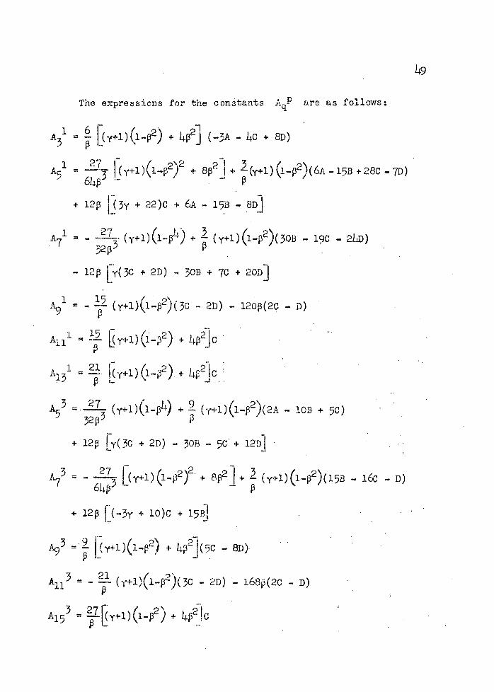
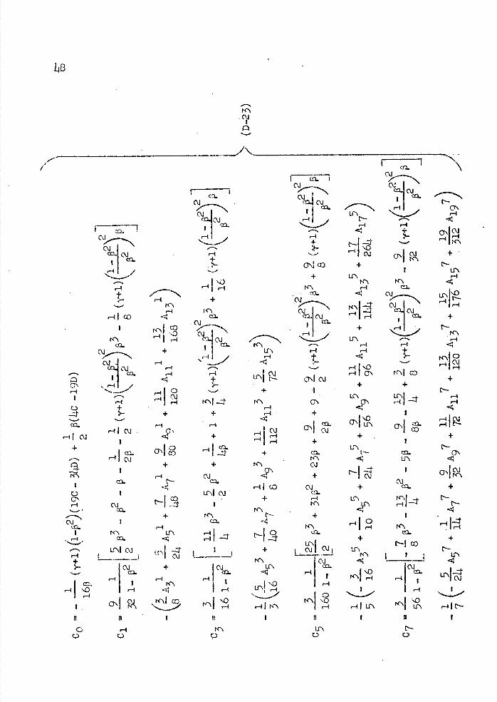
The expressions for the constants AqP are as follows:

A =+ 2] (-3A - + aD)

3 P

= I(y^1)(i_p2)2 + e 2 t + (y+1) (1_p2)(6A - 15B + 28C - 7D)

6t.p - p

+ 12 (3y + 22)C + 6A - 1513 - 8Dj

A71 - L 32 p3

(y+1)(1-p14) + (y+1)1_p2)(30B - 19C - 2L)

- 120 [(3c + 2D) -. 30B + 7C + 20Dj

= - 22 (Y+1)(1_32)(3c 2D) - 120p(2C - D)

[(Y+l)(i_p2) i4p2Jc

A131 = ky+ii- 2) + 4 lc

27 (+i)(i_p14) + 2 (+1)(1_p2)(2A - 103 + 50) 32P3 P

+ 12p Iy(3C + 2D) - 3013 - 50 + 1201

A - 27 f( i+l)(1_p2 )2 + 8p2 ]+ 2 (y+1)(lp2)(15B - 16c - 0) 614p p

+ 12 I(- + io)c + 15Bf

A 3 1R y+1)(1p2) + - 80)

A11 3 = - ! (yi-1)(1_p2)(3c - 2o) - 16813(20 - D)

A153 = L7 A15

+ 421c

149

1 P2

= - (y+1)12)(3A + - GD)

A5 5 - (y1) (i-. 2)c - [e+1) (i = 2 ) + 42 JD

A75 = - ^i (i 2) + (y+1)(i—)(9B -. D)

- 12112C + (2y - 23)D

A95 = - ! (y+i) (1_p2)(C - 2D) 25213C

A, 1 5 = y+i) i 2 ) + - 2D)

A1 - (y+1)(1-23c - 2D) - 216(2C - D)

A17 = +i) (i _2) i c

A5 7 (y+1) (_2)2 - (y+1)(12)(5B + 12C - 29D) + 12(2y + 1)D 64 3 0

A77 (y+1)(12)C - ky^1(1p2) + !2iD

= - 192(C - 2D)

A11 7 - [+i) (i2) - 12 1 C + (y+1)(12)D

A137 2J+1)(i2) + - 2D)

A157 = - j3(y+i)12) + 16P21c + ky+1)1 2) + 42jD

A197 y+1) (,_p2 +

51

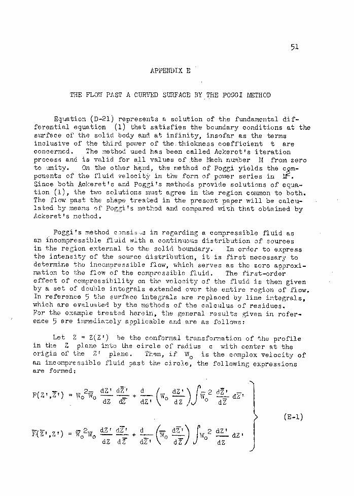
APPENDIX E

THE FLO7 PAST A CURVED SURFACE BY THE POGGI METHOD

Equation (D-21) represents a solution of the fundamental dif-ferential equation (1) that satisfies the boundary conditions at the surface of the solid body and at infinity, insofar as the terms inclusive of the third power of the-thickness coefficient t are concerned. The method used has been called Ackeret's iteration process and is valid for all values of the Mach number H from zero to unity. On the other hand, the method of Poggi yields the com- ponents of the fluid velocity in the form of power series in I.F. Since both Ackeret's and Poggi's methods provide solutions of equa-tion (1), the two solutions must agree in the region common to both. The flow past the shape treated in the present paper will be calcu-lated by means of Poggi s method and compared with that obtained by Acke ret 's method.

Poggi's method cjnsiss in regarding a compressible fluid as an incompressible fluid with a continuous distribution of sources in the region external to the solid boundary. In order to express the intensity of the source distribution, it is first necessary to determine the incompressible flow, which serves as the zero approxi-mation to the flow of the compressible fluid. The first-order effect of compressibility on the velocity of the fluid is then given by a set of double integrals extended over the entire region of flow. In reference 5 the surface integrals are replaced by line integrals, which are evaluated by the methods of the calculus of residues. For the example treated herein, the general results given in refer-ence 5 are immediately aoplicable and are as follows:

Let Z Z(Z') be the conformal transformation of the profile in the Z plane into the circle of radius c with center at the origin of the Z' plane. Then, if VT is the complex velocity of an incompressible fluid past the circle, the following expressions are formed:

= WQ2W0 + (Wc')J2 dP

dZ dZ dZ'\ dZ, ° dZ

(E-l)

= w 2 + =_ (w -;) Jw2 dZ' dZ dZ dZ' dZ dZ

52

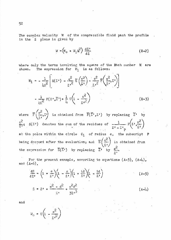
The complex velocity W of the compressible fluid past the profile in the Z plane is given by

= (w0 + wi ') dZI- (E-2) dZ

where only the terms involving the squere of the Mach number M are shown. The expression for is as follows:

-(- _2!_

z Z' \Z', Z! 2 Z

- - F(Z',')+- (E-3)

141J 1 \ 2'\

where Ft -,Z'I is obtained from F(Z',Z') by replacing Z' by

,2 ) \z'J /

; s(z') denotes the sum f the residues of _. F(Zt,E Zt -Z t \ L

at the poles within the circle C 1 of radius c, the subscript P

being dropped after the evaluation; and S( C2 —) is obtained from

2 the expression for () by replacing ' by Q.

For the present example, according to equations (A-3), (A-Q, and (A-6),

d' (1 _;)(i

^\)( _)

(A-3)

c2 -d2 c2d2 z = z' + + 7 (4)

2:' 3Z'

and

wo =

(1 - T)

C"C)

LNI +

Cu

C"

4)

4)

0

-1 0

C"

+

-Th

c'J

c'J

+

+

r1

+

C"

C"

rj

c\JC)

0 ('.1

C"C)

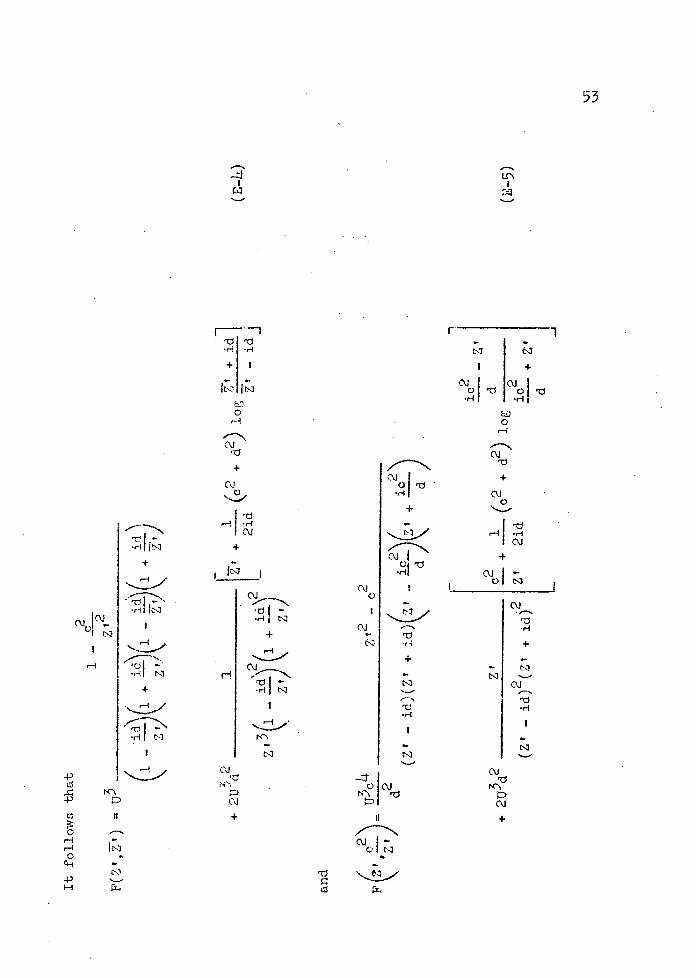
53

r.

r

• H •,1

+ I +

('J .1 0

r1

0C

oJrj

C" +

C"

+ c\J

0.

C"C)

+

cv

r_-, •,-f

rl cd

1

- d2 z'2 + d2(E-6)

54

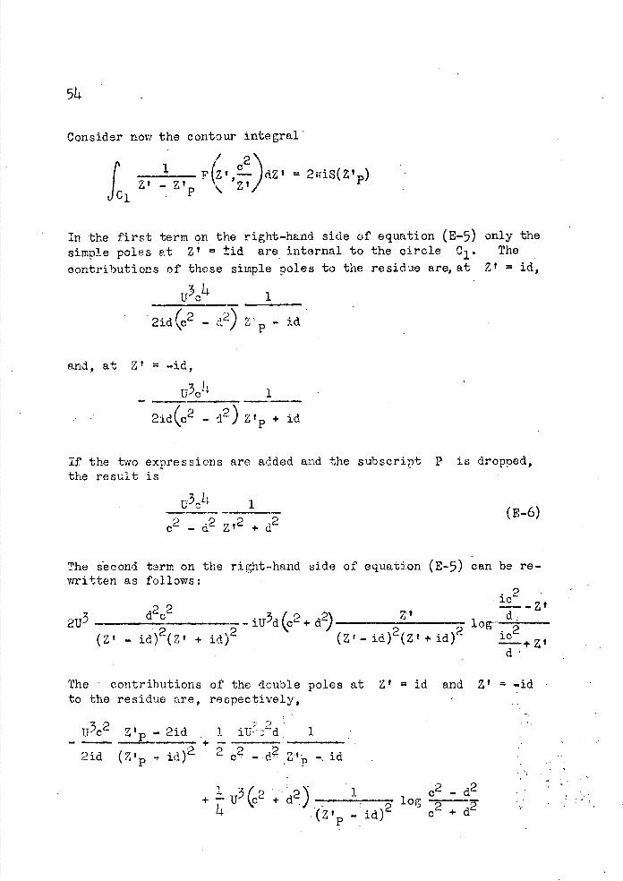
Consid er now the contour integral'

/ 2'

fc;

dZ' = 2TdS(Z')

1zP P( '\

ifl the first term on the right-hand side of equation (E-5) only the simple poles at Z' ±id are internal to the circle C l . The

contributions of those simple poles to the residue are, at Z' id,

U304 1

21d(02 - Z' - id

and, at Z' -id,

21d(C2 -i2) Z' + id

If the two expressions are added and the subscript P is dropped, the result is

The second torm on the right-hand side of equation (E-5) can be re-written as follows:

ic2

2U3 d2c __jUd(c2+d2)2

210 d (z' - id) (z' + id) (Zr- id(Z'+id)

d*

The contributions to the residue are,

173c2 Z' - 2id

2id (z' - Id)a

of the double poles at respectively,

1 iTJ-d 1 4. -2 ?_ d? Z' t -. id

Z' Id and 1' = -id

I 3' 2" •1 c2-d2

+Uc +d) , log 2 14 i - d) c +

0

ii'

55

and

U3c2 Zi p + 2id 1 iU3c2d 1

2 i ( zt + id )2 2 c2 - d2 Z' + id

+ + d2) 1 c2 - d2

•(z'+id)2 c2+d2

If the two expressions are added and the subscript P is dropped, the result is

2Uc2d2 U302d2 I

(t2+d2)2C2d27?2+d2

+ 1 u

2" Z?2 - 2 C2 - d - - + d ) log (E-7) 2(zt2+d2)

If the expressions (-6) and (E-7) are added, it follows that

c2+d2log 2 _a2\ Z,2 - d2 + - s(z') U3 c 2 (1

2c 2 C2 + d) z, 2 + d2)2 (E-8)

From equation (E-t),

- (z'2 2\Z 12T,2

Z 12 12 F(Z' 7t\ = /

+ d2)(T2 + 2)

I 2U-1d / c + d Z' + id

+ - ( Z'Z' + Z' log.— - (E-9) • + d2) '\ 2id ZI- id

If s(') is formed from equation (E-8) and Z' is replaced by

, it follows that

56

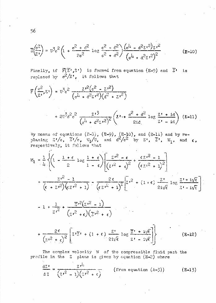
_/2\3 2( c2 + c2 - d\ - a2z,2)z,2

= U c+

logd2)(j. + d2Z?2)

(E-iO)

Finally, if V(,Z') is formed from equation (E-9) and Z' is replaced by 02/Z 1 , it follows that

( 2 ') z'2) 7, t- -c+ d2Z? 2)(d2 + 712)

+ 2U)d2c2 ZT3

22 + d2 log Z' + id\ (E-11)

+ d2Z'2) \\ 21d, - id)

By means of equations ( E-6 ) 1( B-9), (E-lO), and (E-li) and by re- placing z'/, 2v/c, r1/u, and d/c2 by Z, 7 1 , W and €,

respectively, it follows that

+ € i. + €Z, 2 - - i

W1 —<l - lo - - +

2 1 - €) L

+ )2 (€712 + 1)2

- 1 2€ 1 2 ____ Z'+i/

------------"-Z' +I+E ) — log

+ '1%, Z,2+ i) (€z2 + l)[ 2i

1 2(z2-1) - 1 +

+ ( ,2 + +)

+ (2 )2 I'' ^ (1 + €) 2iV

log+

(E-12)

The corimlex velocity W of the comDressible fluid past the Profile in the Z plane is given by equation (E2) where

dZ' 7J4-- =

--- (from equation (A-3)) (E-13) dZ (z t2 - l,)Z'

+ C)

57

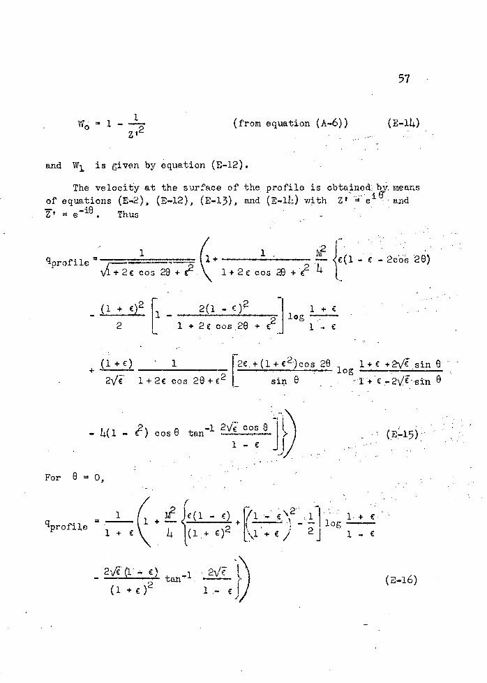
1 - - (from equation (A-6)) (E-lL.)

and WI, is given by equation (E-.12).

The velocity at the surface of the, profile is obtained: br. means of equations (E-2), (E-12), (E-13), and (E-lLi) with Z' ' e ' and

Thus -

profi1e

(+ 2€ + .2

c(l - -. 2cbs 29)

(1 + )2 [ 2(1 - 1 1 + c •, ' ' - l log ..

2 l+2€ cos 29+ € 1-c

L+ (l +c) 1 !2c.+(l+c2)cos 29 log +2Vi.sin 9"

2' 1+2c cos 2+E 2 sin 9. :"

€-2,/€ sjn 0

- (' - cos tan2 co: $

(E15)'

For O=o, . .

+

profiec

+ J(l

c(1€)

log

- 2(1 ) 2(E16)

(1 + 1 .- c I •1

58

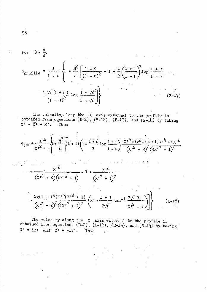
For 8=,

1 i+l(1iog+ €

profile- C 14 -c) 21

(l 'log ('L17)

The velocity along the. X. axis external to the profile is obtained from 'equations (E-2), (E-12), (E-13), and (E-114) by taking

= X'. Thus

r2

X l + €

14 •_ \ 2 1 - €)(x'2 + + 1)2

2 x,-. -1+

(x v2 +C)(x t2 +l) (xt2+c)2

2'c(l - + 1) ( +

2(E-15)

(x'2 + c) 2 (€x 2 + 1) 2 \\ 2'i - €) jJ

The velocity along the Y axis external to the profile is obtained from equations (E-2.), (E-12), (E-13), and (E-114) by taking

ly ' 'd' T, = -iY'. Thus

59

12 t +

___

_(l+)(l _±

1o g _

2 i_c,) ( - __- cyt2)2

Y t4 -

- '2)(i -€y'2) -1

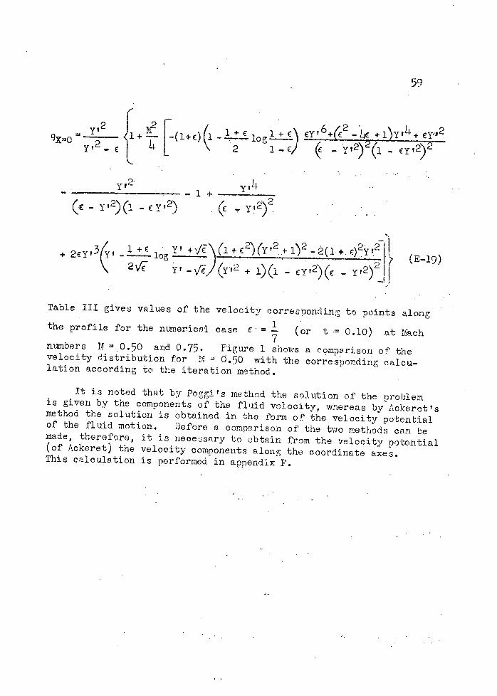
+ 2cYf3(Yt 1 + 1Y' +Vi(i+C2(Y?2+l2^(l;+r)2Y?2li (E-19) \ 2V€ + i)(i - cY v2)(c - y12 2

Table III gives values of the

the profile for the numerical

ntmibers M = 0.50 and 0.75. velocity distribution for L lation according to the itera-

velocity corre s ponding to points along

case = (or t •= 0.10) at Irjach

Figure 1 shows a comparison of the 0.50 with the corresponding calcu-

:ion method.

It is noted that by Pogo-i t s method the solution of the problem is given by the components of the fluid velocity, whereas by Ackeret's method the solution is obtained in the form of the velocity potential of the fluid motion. Before a comparison of the two methods can be made, therefore, it is necessary to obtain from the velocity potential (of Ackeret) the velocity components along the coordinate axes. This calculation is performed in appendix F.

60

APPENDIX F

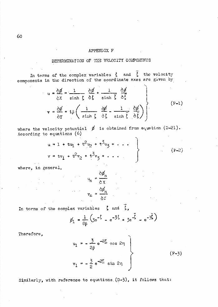
DETERMINATION OF THE VELOCITY COIONENTS

In terms of the complex variables t and i the velocity

components in the direction of the coordinate axes are given by,

• cj +' 1 U

oX

-

sinh O sinh

(p-i)

àY \ inh à sin àJ

where the velocity potential 0' is obtained from equation (D-21). According to equations (6)

ul+tu1 +t2 +t3U3 +. ...

-.

where, in general,

oø,n Ufl

vn:.

(F-2'

In terms of the complex variables and L

i - + 3e - e-3t)

Therefore,

3 -2, * - e cos 21j

2

Vi - e sin 2

Similarly, with reference to equations. (D-3), it follows that:

61,

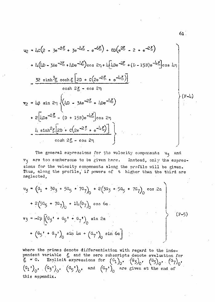
42 = c (2 - 3e 2 + 3e - e 6)

+ 8D (e2 2 + e 1 + L_3Ae 2 +L i e)cos 211^)4[)4De 2 +(D-l5B)ecos 4q1

32 sinh 3 cosh2D + C(2e*2 + e)I cosh 2, - cos 2 TI

72 sin 21 - 3Ae_2 + Le)

+ 2e_2 - (D + 15B)e'jcos 2n

sinh2D '+ C(2e + -)1 -cosh 2 - cos 21j J

The general expressions for the velocity ccmponents u3 and V3 are too cumbersome to be given here. Instead, only the expres-

sions for the velocity components along the profile will be given. Thus, along the profile, if powers of t higher than the third are neglected,

= (G1 + 3G3 + 5G5 + 7G7) + 2(3G3 +. 5G5 + 7G 7) cos 2a

+ 2(5G5 + 7G7) + 14(G7) cos 6a.

V3 -2 [(G3 ' + G5 ' ^G7 ') sin 2a I + (G5 1 + G

77t ) sin La + (G7 T ) sin 6aJ

where the primes denote differentiation with regard to the in-de- pendent variable , and the zero subscripts denote evaluation for

0. Explicit expressions for (c11 ) ' G3), (G5 , (G.7),

(GlO, (G3 i), (G5 t), and (G7 t ) are given at the end of

this appendix;

a)-

a, 4,4)

a,

hO Q)

tj -4

02 0

.0

-P

r—

N.

(U (5 N-

02 o 0

+

----'---' (_'

-p

(U

o

+

c'iI N- cJ +

+1 I

(3

+ +

O\

+i—_

+ _-.--_-r-r,

0_i

co.co.co. t.C\

(U01

++

c_S

-

+

'-I

L° I

NC'J

+

+

CU

<U

•CU -p

4.

I

<____-,

co. +

CO.

+

N-

\O (U

CO.

+

cu

('-I

".4 d

I t • 4.)

ci'IO\1', +

+I

0_i 4-)

+ . NZt C\J

4)

.IC\l

L,J;._ .J

1)

WN

4)

4.)(3

a)

-p + L

C.') u

4'+

a)(3

hO

+ -'-1

-p

+ 0

C)

C) +

0

C'J

-1

$4 "-4

+

-p

-p 0

C)

(I)

E

-P0

—I) C)

"-4 0

\I c0

+

a),

4) .-

U)

as 0 1 .r

63

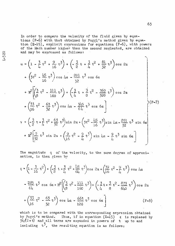
In order to compare the velocity of the fluid given by equa-tions (F-6) with that obtained by Poggi's method given by equa- tion (E-15), explicit expressions for equations (F-6), with powers of the Mach number higher than the second neglected, are obtained and may be expressed as follows:

u ( - t2 ++ t + + tcos 2a \ L. 16 / \

(_ 2 L1. 32

+(32

L1.5 3\\

t -----t ,cosLi.a_2!t 3 cos 6a 16' 32

+ 1/" t2 _!t 3)+ ^2 - tcos 2a369 3)

8 320 ,' 160

+ ( t2 - 32 ) cos ha - t3 \i6

cos 6a1(F-7)

J

2a.+(32 b5 3\ 201 v t+t2+ t3sin t - t )sin La-- t sin 6a 16 ,/ 32

+ 1t3 sin 2a +(2 sin ha -t 3 sin 6a 1 32 '\i6 L ,1

-J

The magnitude q of the velocity, to the same degree of approxi-mation, is then given by

t2) + (_ t + t2 + tcos 2a + ( t2 - t 3 ) cos ha 16 \2 b 64 \16

- t3 cos 6a+ 1( t - t+ t2- J) cos 2a 64 k8 160 / L. 8 6ho

+ (

33 t2 - 3'\ cos L - 663 3 cos 6a (F-a) 16 32 1 128 J

q -

which is to be compared with the corresponding expression obtained by Pogi t s method. Thus, if in equation (E-15) € is replaced by 3t/(2+t and all terms are expanded in powers of t up to and

including t 3 , the resulting equation is as follows;

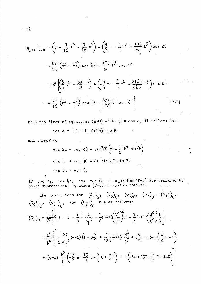
614

(3)

1)profi1e = + 16 l 2 14

cos

+ .L (t2 - o - t3 cos 68 16 "

+ IF t2 - + t +- 2163 cos 20

140 / 8 6140 1

+ 1 - t 3) cos 148 - . 405 t 3 cos 60 (F9) 1 .6 . 128

From the first of equations ( A-9) with X cos a, it follows that

cos a ( 1 - t sin2O) cos 0

and therefore

cos 2a = cos 20 - 81n228(t - t2 sin2e)

cos ij.a cos itO - 2t sin 140 sin 20

cos 6a = cos CO

If cos 2a, cos 14a, and cos Ca in equation (F-B) are replaced by these expressions, equation (F-9) is again obtained.

The expressions for G1 0 , (c)0, (G5)0, (), (G1?),

and @7')

are as follows: 0 0 0

(Gl)O T2 = - 1- - —., ) ^ I

IF 27+1)(lp14) + (Y + + 9 + C D) 567 128

+ (Y+l) A+ 15 B- C + 2 D) + 0 6A + 15B C + 14D

P (- 2 T- 8 2 2

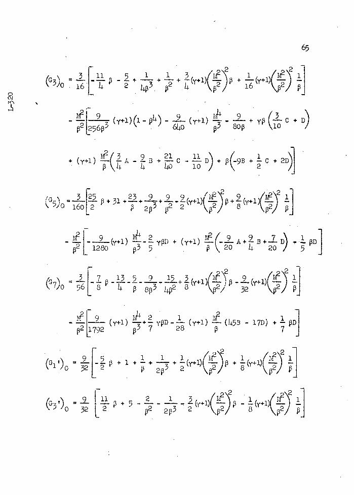
65

(G3) =E ++4+(i+1)() ^fr+i)(4)

- 2[2563 (y^i)(114) -

64o p

L (y+1) + D)

+ ( y+i ) A B +C D)+ P 9 +C +2D)1

2 (G\ 23 9 9 9 + 31 +-+-+

510 16o[2 2+1)()++1)()

(y+1)-yD + (y+1) (A+B+1D

L 1- 1280 3 s 20 14 20 / 5

= [-4+(Y+')(T)'(Y+')() *]

+ [7792

92(y+1) - 1) +

2 28— (Y+l) 7 D]

(G21 2 5 = L 3 + 1

1 1 1 + +-+ 1i)

L 2p _(Y+i)(> + (+i)(P^^)

@3')o = t L 20 2 2p3 2 ' ^,T) 8 (^2)

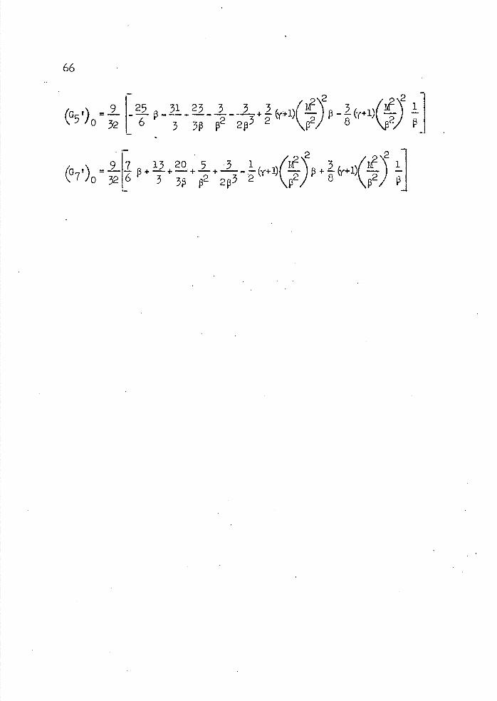
(G5t)=

[ 1

(G7?) = - - 6

13 20 5 •3'2 8 .(p2) 32 3 2 2p3

67

REFERENCES

Ri1. Taylor, G. I.: The Flow of Air at High Speeds past Curved

Surfaces. R. & N. No. 1381, British A.R.C., 1930-

2. Gdrtler, H.: Gasstrmungen mit Ubergang von Unterschall- zu Uberschallgeschwindigkeiton. Z.f.a.M.M., Bd. 20, Heft 5, Oct. l9L0, pp. 254-2.

3. von Krmn, Th.: Compressibility Effects in Aerodynamics. Jour.. Aero. Sci., vol. 8, no. 9, July 1 91.1, pp. 337-356.

Li.. Ackeret, J.: tTber LuftkrKfte bel sehr grosson Geschwiudigkeiten insbesondere hei ehonen StrSmunen. Helvetica Physica Acta, vcl. 1, fasc. 5, 1928, pp. 301-322.

5 . Kaplan, Carl: Or the Use of Residue Theory for Treating the Subsonic Flow of a Compressible Fluid. Rep. No. 728, NACA, 19L2.

68 TABLE I

VELOCITY AND PRESSURE DISTRIBUTIONS A!I' ThE SURFACE OF A BIJ1,1P, t 0.10

o X Y q Cp (deg) (Equation (A-9)) (Equation (A-9)) (Equation (A-b)) (Equation (A-li))

O 1.000 0 .8750 .2344 5 .9954 .0001 .8764 .2318

10 .9818 .0005 .8808 .2241 15 .9595 .0017 .8881 .2113 20 .9287 .0040 .8983 .1931 30 .8444 .0125 .9272 .1404 40 .7344 .0266 .9667 .0654 50 .6051 .0450 1.014 -.0292 60 .4625 .0650 1.068 -.1395 70 .3118 .0830 1.117 -.2476 80 .1568 .0955 1.15 -.3299 90 0 .1000 1.167 -.3611

TABLE II

VALUES FOR A, B, C, AND D OBTAINED FROM EQUATION (D-3)

M B A B C D

0 1 0.06250 -0.06250 0 0 .10 .99499 .06221 -.05285 .00095 0 .20 .97980 .06160 .06390 .00400 .00015 .30 .95394 .06169 -.06570 .00982 .00083 .40 .91652 .06499 -.03830 .01990 .00307 .50 .88603 .07786 -.07171 .03751 .00939 .60 .80000 .11322 -.07551 .07057 .02675 .70 .71414 .24561 -.07741 .14211 .07805 .75 .65144 .40177 -.07394 .21371 .13977 .80 .60000 .73343. m.06322 .34482 .26722 .83 .55776 1.11855 -.04583 .48400 .41460 .85 .52678 1.53475 -.02476 .62619 .57315 .90 .43589 4.07940 .12446 1.4241 1.5367 .92 .39192 6.81182 129917 2.2282 2.5674 .94 .34117 12.9343 .70926 3.9598 4.8722 .96 .28000 31.0576 1.97342 8.8910 11.683 .93 .19900 132.428

I9.30328 34.423 49.732

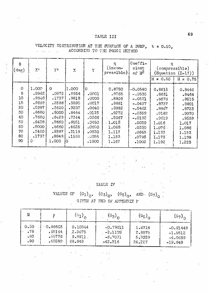
TABLE III 69

VELOCITY DISTRIBUTIOT AT TME SURFACE OF A BU, t 0.10, ACCORDI1G TO T:1E POGGI 1-11ETHOD

8 (dog)

q (incom-.

pressible)

Coeffi- dent of M2

q (compressible)

(Equation (E-17))

M = 0.50 Ill = 0.75

0 1.000 0 1.000 0 0.8750 -0.0540 0.8615 0.8446 5 .9962 .0872 .9954 .0001 .8765 -.0535 .8631 .8464

10 .9848 .1737 .9818 .0005 .8808 -.0521 .8678 .8515 15 .9659 .2588 .9595 .0017 .8881 -.0497 .8757 .8601 20 .0397 .3420 .9237 .0040 .8983 -.0462 .8867 .8723 30 .8660 .5000 .8444 .0125 .9272 -.0359 .9182 .9070 40 .7660 .6429 .7344 .0266 .9667 -.0192. .0610 50 .6428 .7660 .6051 .0450 .1.015 .0039 1.016 1.017 60 .5000 .8660 .4625 .0650 1.068 .0330 1.07 1.086 70 .3420 •93971 .3118 0830 1.117 .0645 1.133 1.153 80 .1737 .9848 .1563 u955 1.15:3 .0795 1.173 1.198 90 10 1.000 0 .1000 1.167 .1002 1.192 1.223

TABLB 111

VALUES OF (G1)0, .(03)0, (G5) 0 , AND (G7)0

GIYBU AT END OF APPENDIX F

(&i). (G3)0 (5)0 (G7)0

0.50 0.86603 0.10344 -0.79011 .1.6714 -0.91449 .75 .65144 .2.3075 -2.1139 2.8975 -1.9512 .83 .55776 9.8911 -6.7071 5.9329 -4.0650 .90 .43580 68.849 -42.316 26.227 -19.649

70 TABLE .V

VALUES OF a, a2 , AND a3 OBTAINED FROM EQUATIONS(14)

0.50 0.75 0.83 0.90

0 1.7321 2.3026 2,6893 3.4412 1 1.6974 2.2565 2.6355 3.3724 0 1.5935 2.1184 1 2.4742 3.1659

.3 1.4203 1.8881 2.2052 2.8218

.4 1.1778 1.5658 1.8287 2.3400

.5 .86603 1.1513 .1.3447 .. 1.7206

.6 .48497 .64473 .75301 .96355

.7 .03464 .04605 .05379 .06882

.8 . -.48497 . -04473 -.75301 1 -.96355 -1.0739 . -1.4273 -1.6674 -2.1336

.975 -1,5610 -2.0752 -2.4237 -3.1014 1.0 -1.7321 -2.3026 -2.6893 -3.4412

a2

0 2 i 2743 543501 10.136 19.268 - .1 2.0399 4.9892 9.3921 18.076 .2 1.3673 3.7088 7.2538 14.643 .3 I .34809 1.7641 4.0015 9.4302

-.86531 -.56063 .10228 3.1662 .5 -2.0593 -2.8678 -3.7900 -3.1035 .6 -2.9594 -4.6459 -6.8342 -8.0405 .7 -3.2325 -5.2746 -8.0105 -10,022 .8 -2.4744 -4.0011 -6.0811 -7.0773 .9 -.23520 .01270 .33212 2.9861 .975 2.7276 F4013 9.0381 16.723

1.0 4.0063 7.7376 12.825 22.708

a3

0 3.4379 21.877 72.397 47.84 .1 2.5124 18.507 63.333 386.94 .2 .07542 9.4933 38.871 251.93

3 -2.9313 -2.1171 6.6216 72.788 .4 -5.1915 -12.039 -22.646 -92.533

• .5 -5.3952 -15.937 -37034 -184.67 .6 -2.7710 -11.097 01.701 -164.59 .7 2.2311 1.4456 -5.9844 -41.555 .8 7.0916 14.256 22.646 92.580 .9 6.2552 10.459 14.506 23.206 .975 -.82172 -20.694 -56.978 -385.70

1.0 -10.033 -39.831 7101.38 1633.92

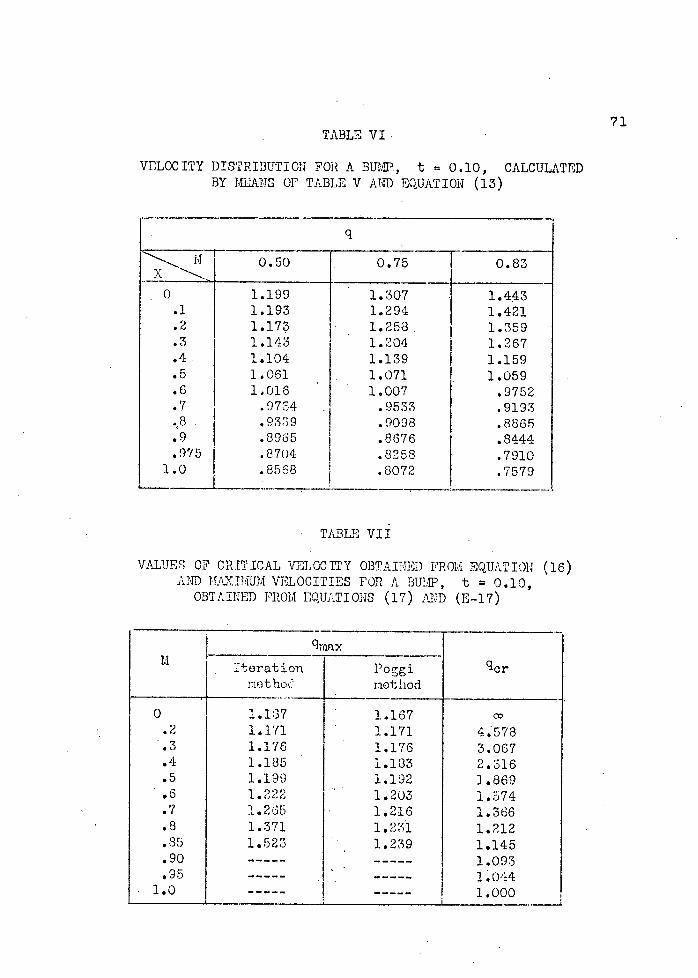
TABLE VI.

VELOCITY DISTRIBUTION FOR A BUTVU'., t 0.10, CALCULATED BY MANS OF TABLE V AND EQUATION (13)

q

1r0.50 . 0.75 1 0.83

0 1.199 1.307 1.443 .1 1.193 1.294 1.421 .2 1.173 1.258. 1.359 .3 1.143 1.204 1.267 .4 1.104 1.139 1.159 .5 1.051 . 1.071 1.059 .6 1.016 1.007 .9752 .7 .9734 .953 .3 .919 3

.9339 .9098 .8865 .9 .8965 .85'76 .8444 .975 .8704 .8258 .7910

1.0 .8568 .0072 .7579

TABLE VII

VALUES OF CRITICAL VELOCITY OBTAINED FROM EQUPT ION (is) AND NAXIMUM VELOCITIES FOR A BUMP, t = 0.10,

OBTAINED FROM EQUATI ois (17) AND (E-17)

qmaxq cr Iteration Poggi

!lot hoc riothod

0 1.157 1.167 cc .2 1.171 1.171 4.578 .3 1.176 1.176 3.067 .4 1.185 1.133 .2.316 .5 1.199 1.192 1.869 .6 1.222 1.203 1.574 .7 1.255 . 1.216 1.366 .8 1.371 1.231 1.212 .85 1.523 1.239 1.145 .90 1.093 .95 1.O't4

1.0 1.000

71

72 TABLE VIII

VALUES OF q/qcr FOR A BUMP, t 0.10, WITH Ii = 0.83

X

0 1.443 1.230 .1 1.421 1.211 .2 1.359 1.160 .3 1.267 1.080 .4 10159 .9881 .5 1.059 .9028 .6 .9752 .8314. .7 .9193 107837 .8

08865 .7558

.9 .8444 .7200

.975 .7910 .6744 1.0 .7579 .6461

TABLE IX

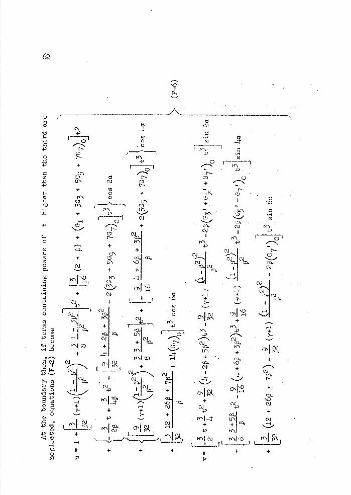
C0IARISON OF TIF, PRESSURE DISTRIBUTION AT TI SURFACE OF A BUIfl, t 0.10 FOR M 0.63 OBTAINED BY RANS ,OF,TI ITERAT ION, T1II PRA1mTL-GLAUERT,

AND T1Th VC)" KAPJ'IAN METHODS

Cp,M

Iteration Prandii- von Iarinan X method Glauert method • (Equation (o)) method

0 •. -0.9133 -0.6342 -0.7376 -0.3537 .1 I -.8677 -.6142 -.7107 -.3426 .2 -.7389 -.5558 -.6337 -.3100

• .3 -.5486 -.4665 -.5202 -.2602 .4 -.3294 -.3514 -.3810 -.1960 .5 -.1184 -.2150 -.2257 -.1199 .6 .0514 -.0647 -.0656 -.0361 .7 .1617 .0765 .0752 .0426 1 8 .2221 • .2062 .1972 .1150 .9 .2868 .3196 .2983 . .1783 .975 • .4048 • .3935.' .3620 .2195

1.0 .4708 • .......4163 •:3] .2322

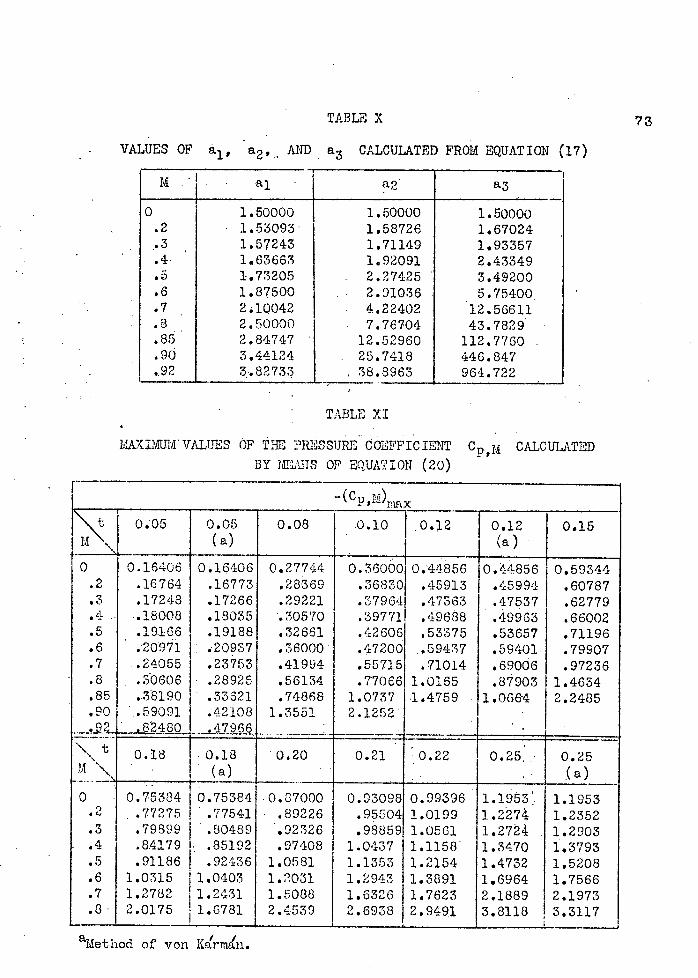
TABLE X 73

VALUES OF a, a2 , AND a3 CALCULATED FROM EQUATION (17)

.M.. . al a2. a3 -

O 1.50000 1.50000 1.50000 .2 1.53093 1,58726 1.67024 .3 1.57243 1.71149 1.93357 .4 1.63663 1.92091 2.43349 .5 1.73205 2.27425 3.49200 .6 1.87500 . 2.91036 5.75400. .7 . 210042 4.22402 12.56611 .8 2.50000 . 7.76704 43.7829 .85 2.84747 12.52960 112.7760 .90 3.44124 . 25.7418 446.847 .92 . - 3.82733 - 38.5963 964.722 -

TABLE XI

MAXIMUM VALUES OF TuE PRESSURE COEFFIC lENT C ,j CALCULATED BY JVflIUTS OF EQUATION (20)

t 0.05 0.05 0.08 .0.101 .0.12 J 0.12 0.15

(a)

0 0.16406 0e16406 0.27744 0.36000 0.44856 10.4,S856 0.59344 .2 .16764 .16773 .28369 .36830 .45913 .45994 .60787 .3 .17248 .17266 .29221 .37964 .47363 .47537 .62779 .4 ... .18008 .18035 .30570 .39771 .49688 .49963 .66002 .5 .19.166 .19188 .32661 !42606 .53375 .53657 .71196 .6 .20971 : 20937 .36000 .47200 .59437 .59401 .79907 .7 .24055 .23753 .41994 .55715 .71014 .69006 .97236 .8 . .30606 . .28925 .56134 .77066 1.0165 .87903 1.4634 .85 .38190 .74868 1.0737 .1.4759 . 1.066-4 2.2485 .90 .59091 .42108 1.3551 2.1252

2480

\ 018 . 0.18 0.20 0.21 0.22 0.25.. 0.25 IA \ . (a)

0 . 0.75384 0.75384 . 0.37000 0.03098 0.99396 1.1953. 1.1953 .2 . .77275 .77541 .89226 .95504 1.0199 1.2274 1.2352 .3 .79699 .80489 .92326 .98859 1.0561 1.2724 . 1.2903 .4 .84179 .. .85192 .97408 1.0437 1.3470 1.3793 .5 . 91186 .92436 1.0581 1.1353

11.1158* 1.2154 1.4732 1.5208

.6 1.0315 1.0403 1.2031 1.2943 11.31391 1,6964 1.7566

.7 1.2702 1.2431 1.5088 1.6326 1.7623 2.1889 2.1973

.8 2.0175 1.6781 2.4539 2.6938 2.9491 3.8118 I 3.3117

' aMetIod of von Karmfn.

74 TABLE XII

CRITICAL AND LIMITING VALUES OF IA AND CRITICAL VALUES OF Cp,M CALCULATED DY AEANS OF EQUATION (21)

M _(Cp,M)cr t -C Poe Mcr Mum

0.45 2.70639 . 0.05 0.16406 0.832 0.890 0.50 .50 2.0953 .08 .27744 .775 .855 .77 .55 1.65519 410. .36000 .742 .833 .92 .60 1.29190 .12 .4485 . .712 .815 1.09 .65 1.00661 .15 .59344 .670 .790 1.33 .70 477758 .18 .75384 .634 .760 1.58 .75 .59008 .20 .87000 .610 .743 1.74 .80 .4381 .21 . .93098 .598 .735 1.82 .85 .30124 .2. .99396 .587 .725. 1190 .90 .18605 .25 1.1953 .558 .698 2.15 .95 .08783

_1.00 0

TABLE XII I

VALUES OF ThE PRESSURE COEFFICIENT (Cp,M)abs CALCULATED

BY MEANS OF EUAT ION 1 22)

N -.(Cp,M)bS . M .

0.70 2.90508 .. 1.25 .91103 .75. . 2.53064 . 1.30 .84230 .80 2.22420 . 1.35 .78106 .85 1.97022 1.40 .72627 .90 1.75739 1.45 07705 095 1.57727 . 1.50 .63266

1.00 1.42349 1.55 .59250 1.05 1.29115 1.60 .55605 1.10 1.17644 1.65 .52286 1.15 1.07636 1.70 .49256 1.20

J.98853 1.75 .46481

uiauiiauiiuimusi uaiaiuuivaiO

EMiaauaa

MEMO M MEN ON MEM

UiiUIRUkUSIlIR

U. Iu.iiaiiiiaa ImI.Iu'vAmL'aR

• gi $

I. v iik 17 MEWS

I

iI_-___UIIiL AU.iIIvIIIiiIImIauuai

q

L.E

1.4

1.2

1.]

l.(

NACA

Fig.. 1

Y.

1.6

1.4

1.2

1.0

.8

.4

.2

0 0 .2 .4 .6 .8 1.0

x

Figure 1.- Velocity distribution at the surface of a bump, t = 0.10, for several values of the Mach number.

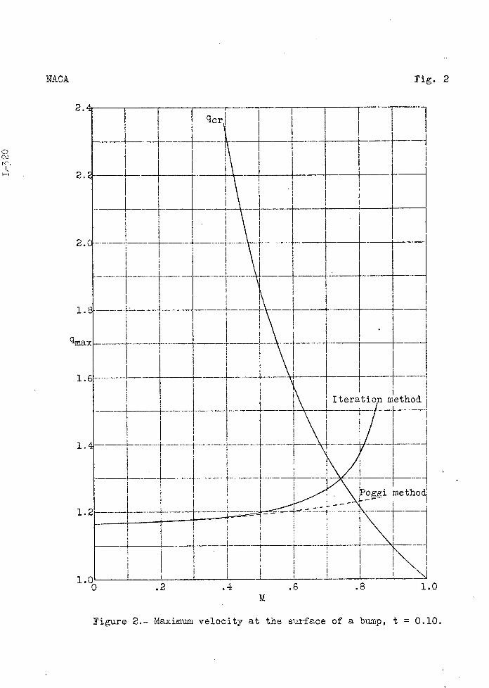
Figure 2.- Maximum velocity at the surface of a bump, t = 0.10.

NACA Fig. 2

.2.

.6 .8 1.0 M

C) (\1

2.

2.4

2.0

1.00

-El :1'-p IIi1 _ -- -\- --_ --H-- --4---- -- ---- Iteratio rn'ethod.

-

JPoggi method. ±tI:IIzITIEIII I

I

..-. •_•••••__•• - - - -- -

- -.- -

IIIIIIIIIIIIII: - tj

.--,--4

-- -

- on Krrnan method. -. -Prandtl-Glauert method teration method_

C? ,

-.6

-.'

[a

.<

.4

.6

NACA

C (\j

I

Fig. 3

0 .2 .4 .6 .8 1.0 1.2 1.4 1.6 A

Figure 3.- Pressure distribution at the surface of a bump, t 0.10, for M = .83.

ITACA 4

-2.E

-2. oJ

-.

-l.

-1.i

( Op , M) ma:

-1.

-1.

-1.

I _LJ_iI1I 1 J. r critical prs-sure coefficient at which (OM)abs I

- local fluid speed equals

-I

- --

I 1local speed of sound.

(cP,M) urn :: limiting - value of pressure coeffi - - -- -

i - - v Y") iim cient beyond which flow -without shock cannot - - -

.* exist.t t—IH

(

,M) abs: absolute

-_' ---•_•

i- / lirnitin pressure

. 22 ';___' coefficient; that is to a corresponding

-

/ \ vacuurn.j I J_ I . I \ _____ Results of present .18 paper Results-of von L---\J

:---- • xarman

III

II - B H1--- - 08

'

2.

T±IIIrI L... -•.- \r•-----+--- -

.0 .2 .4 .6 .8 1.0 1.2 1.4 1.6

M

Figure 4.- Maxinrm pressure coefficient as a function of the Mach number.