1188 ieee transactions on image processing, vol. 26, no. …big › publications ›...

1188 IEEE TRANSACTIONS ON IMAGE PROCESSING, VOL. 26, NO. 3, MARCH 2017

Multiresolution Subdivision SnakesAnaïs Badoual, Daniel Schmitter, Virginie Uhlmann, and Michael Unser

Abstract— We present a new family of snakes that satisfy theproperty of multiresolution by exploiting subdivision schemes. Weshow in a generic way how to construct such snakes based onan admissible subdivision mask. We derive the necessary energyformulations and provide the formulas for their efficient compu-tation. Depending on the choice of the mask, such models havethe ability to reproduce trigonometric or polynomial curves. Theycan also be designed to be interpolating, a property that is usefulin user-interactive applications. We provide explicit examples ofsubdivision snakes and illustrate their use for the segmentation ofbioimages. We show that they are robust in the presence of noiseand provide a multiresolution algorithm to enlarge their basinof attraction, which decreases their dependence on initializationcompared to singleresolution snakes. We show the advantages ofthe proposed model in terms of computation and segmentationof structures with different sizes.

Index Terms— Multiresolution, subdivision, snake, minimum-support, Deslauriers-Dubuc, segmentation, interpolation.

I. INTRODUCTION

ACTIVE contours, also called “snakes”, are popular mod-els for the segmentation of biomedical images [1]–[6].

They consist in an initial shape that evolves towards theboundary of the object of interest. The evolution is guidedby the choice of an appropriate energy term to be minimized.Different snake models have been proposed [7], [8]. They canbe categorized by the way their shape is described: eitherdiscretely or in the continuous domain. In particular, thereare point-snakes and parametric snakes. Point-snakes havea simple discrete representation. The shape is described bya set of ordered points [9]. However, they rely on a largenumber of parameters (i.e., the snake points), which requiresan internal regularization to enforce smooth boundaries andmakes the optimization more challenging. Parametric snakeshave a continuous representation by using basis functions.They require fewer parameters (i.e., control points), whichresults in a faster optimization and better robustness. They areusually built in a way that ensures continuity and smoothness.However, the shape that the snake can reproduce is limited byits parametrization. We propose in this paper a geometric rep-resentation that combines the advantages of point-snakes andparametric snakes. In our representation, the curve is driven bya discrete set of a few master points, called control points, that

Manuscript received April 27, 2016; revised September 28, 2016 andDecember 1, 2016; accepted December 13, 2016. Date of publication Decem-ber 21, 2016; date of current version January 20, 2017. This work wassupported by the Swiss National Science Foundation under Grant 200020-162343. The Associate Editor coordinating the review of this manuscript andapproving it for publication was Prof. Gustavo Kunde Rohde.

The authors are with the Biomedical Imaging Group, École PolytechniqueFédérale de Lausanne, 1015 Lausanne, Switzerland.

Color versions of one or more of the figures in this paper are availableonline at http://ieeexplore.ieee.org.

Digital Object Identifier 10.1109/TIP.2016.2644263

are the parameters of the model. Then, slave points describingthe curve are generated by specific iterative procedures. Theproperty that makes it possible is called subdivision [10]–[13].It is tightly linked to the theory of wavelets [14] and allowsone to describe a contour or a surface by an initial discreteand finite set of control points which, by the iterative appli-cation of refinement rules, becomes continuous in the limit.The discrete nature of the representation is convenient inpractical applications. At the same time, it implicitly yields acontinuously defined model whose smoothness depends on theparticular choice of the subdivision mask. The main benefitsof subdivision schemes are their simplicity of implementation,the possibility to control their order of approximation, andtheir multiresolution property, which allows for the contour ofa shape to be represented at varying resolutions.

The use of subdivisions for the construction of segmentationmodels was pioneered by [15] and [16] for Doo-Sabinsurfaces [17] and the DLG-scheme [18], respectively. In thefirst case, left ventricles are modeled whereas, in the secondcase, they improved editing semantics of traditional snakes.In this paper, we propose a general approach that remains validfor any subdivision scheme as we derive the construction ofa 2D subdivision snake in a generic way. The primary contri-butions of this work are: 1) a new geometrical representationbased on subdivision. A crucial aspect is the choice of thesubdivision mask that determines important properties of themodel such as its approximation properties, the capability ofreproducing circular, elliptical, or polynomial shapes [19], aswell as the possibility of being interpolatory [20], [21] or not;2) the derivation of associated energy functions such as region-and edge-based terms; 3) the presentation of an integratedstrategy where the snake is optimized in a coarse-to-finefashion. This multiscale approach is algorithmic and inherentlyrecursive: We increase the number of points describing thecurve as the algorithm progresses to the solution; at each step,the scale of the image feature (on which the optimization isperformed) is matched to the density of the point cloud. Thisspeeds up the computation and increases the robustness.

We give several examples of explicit constructions ofsubdivision snakes. We illustrate their use on real imagesas well as on test data simulating real biological conditions.We compare our proposed model to existing parametric snakesand measure its robustness and accuracy w.r.t. noise andinitialization. Specifically, we show that the proposed coarse-to-fine approach allows the optimizer to 1) have a largerbasin of attraction which makes it robust to initial conditions;2) escape some local optima; 3) be efficient by progressivelyincreasing the snake resolution; 4) delineate structures ofdifferent sizes contained within an image without having toadapt the initialization.

1057-7149 © 2016 IEEE. Personal use is permitted, but republication/redistribution requires IEEE permission.See http://www.ieee.org/publications_standards/publications/rights/index.html for more information.

BADOUAL et al.: MULTIRESOLUTION SUBDIVISION SNAKES 1189

A. Organization of the Article

In Section II, we introduce and describe the theory ofsubdivision that is relevant to the construction of curves.In Section III, we fully specify the construction of genericsubdivision snakes. We also describe the proposed multireso-lution algorithm for the optimization. In Section IV, we presentseveral types of multiresolution snakes where the subdivisionmasks possess various properties such as being interpolatory,having different sizes of support, and reproducing polynomi-als. In Section V, we show how subdivision schemes can beused to reproduce trigonometric functions for the constructionof elliptic and circular curves. In Section VI, we perform anextensive validation of subdivision snakes based on test datawhere the ground truth is known as well as on real biologicaldata. Finally, in Section VII, we discuss the choice of thesubdivision mask according to the application and we providea method to choose the parameters of the multiresolutionalgorithm.

II. CLOSED SUBDIVISION CURVES

A. Notations

We represent by p[·] a discrete sequence of points p[m] =(p1[m], p2[m]), indexed by m ∈ Z, where p1 and p2are the corresponding coordinates. We write p(k)[·] =(p1(k)[·], p2(k)[·]) to describe a (2k N0)-periodic sequence,k ≥ 0, with the property that p(k)[m + n2k N0] = p(k)[m],∀n ∈ Z. The discrete convolution of p(k)[·] with a scalar maskh[·] is defined as

(h ∗ p(k))[m] =+∞∑

n=−∞h[m − n]p(k)[n].

B. Subdivision Schemes

A subdivision scheme generates a continuously definedfunction as the limit of an iterative algorithm that is appliedto an initial set of N0 control points. A refinement rule isapplied repeatedly k times to double the number of points ateach iteration, ultimately yielding a set of 2k N0 points. Notethat, at each iteration, the new set of points does not necessarycontain the previous ones. The subdivision scheme is said to beconvergent when the set of points converges to the continuouscurve r = (r1, r2) with r1, r2 ∈ C0 as k → ∞.

A closed curve at resolution k is represented by a (2k N0)-periodized coordinate sequence p(k)[·]. The refinement rulefrom (k − 1) to k is defined by

p(k)[m] = h ∗ p(k−1)↑2[m], (1)

where h is the subdivision mask of the subdivision scheme [22]and ↑2 denotes an upsampling by a factor of 2, given by

p(k)↑2[m] =

{p(k)[n], m = 2n

0, otherwise.

In practice, the mask h has a finite number of non-zeroelements so that the infinite sum in (1) is often reduced toa finite one. Applying (1) iteratively, we can express therefinement rule as a function of the initial set of control

Fig. 1. Flowchart of a subdivision scheme. The periodic sequence p(k),associated to the subdivision points at iteration k, converges to the continuouscurve r; h is the subdivision mask and the sequence h0→k , defined by (3),allows one to obtain p(k) directly from the initial set of control points p(0).

points p(0). The subdivision points at the kth iteration (k ≥ 1)are thereby described by

p(k) = h0→k ∗ p(0)↑2k

, (2)

where

h0→k = h↑2k−1 ∗ h↑2k−2 ∗ · · · ∗ h↑2 ∗ h. (3)

The derivation of (2) is given in Appendix A. Note thateach set of points p(k) is encoded with the N0 control points{p(0)[m]}m∈[0...N0−1]. The subdivision scheme is illustrated inFigures 1 and 2.

In the following, the term control points designates the N0initial points {p(0)[m]}m∈[0...N0−1] and the term subdivisionpoints describes the 2k N0 points {p(k)[m]}m∈[0...2k N0−1] at thekth iteration (k ≥ 1).

C. Convergent Subdivision Schemes

Let h be a subdivision mask with z-transform1 H (z) =∑n∈Z

h[n]zn . A necessary condition for the correspondingsubdivision scheme to be convergent is that

∑n∈Z

h[2n] =∑n∈Z

h[2n + 1] = 1 [23]. The subdivision scheme thusreproduces constants and H (z) = (1 + z)B(z), where B(z) isa Laurent polynomial and B(1) = 1 [24].

For any convergent subdivision scheme, the points of thesequence p(k), as k → ∞, sample the limit curve r, in thesense that [24]–[26]

r(t)∣∣t= m

2k= p(k)[m]. (4)

When the coordinates function of the curve satisfy r1, r2 ∈ C1,the derivative r = dr

dt is also sampled by

r(t)∣∣t= m

2k= 2k(p(k)[m + 1] − p(k)[m]) (5)

in the limit case k → ∞ [25], [27]. The derivation of (5) isgiven in Appendix B. A necessary and sufficient condition fora subdivision scheme to converge uniformly to a continuouslimit function is [23], [27]

⎧⎪⎪⎨

⎪⎪⎩

H (1) = 2

H (−1) = 0

maxm

|h0→k[m + 1] − h0→k−1[m]| −→k→+∞ 0.

In practice, six iterations are enough to have satisfactoryconvergence (see Figure 2).

1This is the conventional definition of the z-transform used in subdivisiontheory.


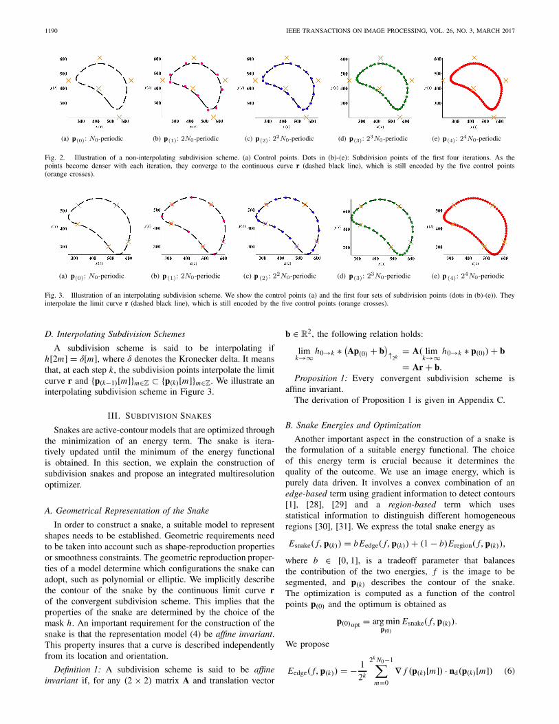
Fig. 2. Illustration of a non-interpolating subdivision scheme. (a) Control points. Dots in (b)-(e): Subdivision points of the first four iterations. As thepoints become denser with each iteration, they converge to the continuous curve r (dashed black line), which is still encoded by the five control points(orange crosses).

Fig. 3. Illustration of an interpolating subdivision scheme. We show the control points (a) and the first four sets of subdivision points (dots in (b)-(e)). Theyinterpolate the limit curve r (dashed black line), which is still encoded by the five control points (orange crosses).

D. Interpolating Subdivision Schemes

A subdivision scheme is said to be interpolating ifh[2m] = δ[m], where δ denotes the Kronecker delta. It meansthat, at each step k, the subdivision points interpolate the limitcurve r and {p(k−1)[m]}m∈Z ⊂ {p(k)[m]}m∈Z. We illustrate aninterpolating subdivision scheme in Figure 3.

III. SUBDIVISION SNAKES

Snakes are active-contour models that are optimized throughthe minimization of an energy term. The snake is itera-tively updated until the minimum of the energy functionalis obtained. In this section, we explain the construction ofsubdivision snakes and propose an integrated multiresolutionoptimizer.

A. Geometrical Representation of the Snake

In order to construct a snake, a suitable model to representshapes needs to be established. Geometric requirements needto be taken into account such as shape-reproduction propertiesor smoothness constraints. The geometric reproduction proper-ties of a model determine which configurations the snake canadopt, such as polynomial or elliptic. We implicitly describethe contour of the snake by the continuous limit curve rof the convergent subdivision scheme. This implies that theproperties of the snake are determined by the choice of themask h. An important requirement for the construction of thesnake is that the representation model (4) be affine invariant.This property insures that a curve is described independentlyfrom its location and orientation.

Definition 1: A subdivision scheme is said to be affineinvariant if, for any (2 × 2) matrix A and translation vector

b ∈ R2, the following relation holds:

limk→∞ h0→k ∗ (

Ap(0) + b)↑2k

= A( limk→∞ h0→k ∗ p(0)) + b

= Ar + b.Proposition 1: Every convergent subdivision scheme is

affine invariant.The derivation of Proposition 1 is given in Appendix C.

B. Snake Energies and Optimization

Another important aspect in the construction of a snake isthe formulation of a suitable energy functional. The choiceof this energy term is crucial because it determines thequality of the outcome. We use an image energy, which ispurely data driven. It involves a convex combination of anedge-based term using gradient information to detect contours[1], [28], [29] and a region-based term which usesstatistical information to distinguish different homogeneousregions [30], [31]. We express the total snake energy as

Esnake( f, p(k)) = bEedge( f, p(k)) + (1 − b)Eregion( f, p(k)),

where b ∈ [0, 1], is a tradeoff parameter that balancesthe contribution of the two energies, f is the image to besegmented, and p(k) describes the contour of the snake.The optimization is computed as a function of the controlpoints p(0) and the optimum is obtained as

p(0)opt = arg minp(0)

Esnake( f, p(k)).

We propose

Eedge( f, p(k)) = − 1

2k

2k N0−1∑

m=0

∇ f (p(k)[m]) · nd(p(k)[m]) (6)


as the edge-based energy, where p(k)[m] is the locationof the m-th subdivision point and where ∇ f (p(k)[m]) andnd(p(k)[m]) are the within-plane gradient of the image f andthe approximation of the normal vector, respectively. The

vector nd =(

nd,1nd,2

)is defined by

nd(p(k)[m]) =(

2k(p2(k)[m + 1] − p2(k)[m])−2k(p1(k)[m + 1] − p1(k)[m])

)

and converges to

nd(p(k)[m]) −→k→∞ n(r(t)

∣∣t= m

2k) =

⎛

⎝r2(t)

∣∣t= m

2k

−r1(t)∣∣t= m

2k

⎞

⎠, (7)

where n(r) is the vector normal to the curve r. The mainadvantage of using (6) instead of only using the imagegradient is that (6) incorporates information about thedirectionality in its expression through the vector nd. Thisallows the snake to discriminate on which side of an objectit is located (e.g., inside or outside of an object).

The region-based energy that we propose discriminates anobject from its background by building a curve rλ around thesnake r, obtained by dilating it by a factor

√2 with respect to

its center of gravity. Then, the contrast is maximized betweenthe intensity of the data averaged over the surface � enclosedby the curve r, and the intensity of the data averaged over theshell �λ\�, where �λ is the surface enclosed by the curve rλ.Note that � ⊂ �λ and |�λ| = 2|�|. The region-based energyis expressed as

Eregion( f, p(k)) = 1

2k |�(p(k))|

×(

22k N0−1∑

m=0

g1(p(k)[m])nd,1(p(k)[m])

−2k N0−1∑

m=0

g1(pλ(k)[m])nd,1(pλ(k)[m]))

,

(8)

where pλ(k) is the sequence of subdivision points that describesthe curve rλ and g1 is the pre-integrated image along thefirst dimension defined by g1(p1, p2) = ∫ p1

−∞ f (τ, p2)dτ . Wedefine �(p(k)) as

�(p(k)) = 1

2k

2k N0−1∑

m=0

p1(k)[m]nd,1(p(k)[m]). (9)

The image g1 is precomputed and stored in a lookuptable, which dramatically speeds up the computation of thealgorithm.

Proposition 2: As k → ∞, the energies defined by (6), (8),and (9) converge to

Eedge( f, p(k)) −→k→∞ −

∫ N0

0∇ f (r(t)) · n(r(t))dt

and

Eregion( f, p(k)) −→k→∞

1

|�|( ∫∫

�f (r)dr1dr2

−∫∫

�λ\�f (r)dr1dr2

),

with

�(p(k)) −→k→∞ � =

∫∫

�dr1dr2,

where � and �λ are the surfaces enclosed by the curve rand rλ, respectively, and � is the signed area enclosed by thecontour r.

These are the standard energies given in [32] and [33]. Theproof of Proposition 2 is given in Appendix D.

C. Multiresolution Approach

The segmentation outcome, when using active-contour mod-els, depends on the initialization of the snake. A largerbasin of attraction allows for a rougher initialization. Withcommon singleresolution segmentation algorithms, a tradeoffhas to be made between the desired accuracy and the amountof blurring one applies to an image. Blurring enlarges thebasin of attraction but also decreases the resolution of anobject, which in turn affects the quality of the delineation.Multiresolution approaches are powerful methods to speedup the optimization process and improve robustness. Existingmethods mainly rely on the construction of an image pyramid,where the active contour is upsampled from a coarse scale toa finer scale of the image [34]–[36]. One limitation of thosemethods is that the object to segment may not have the sametopology on the coarsest and finest images. In this section, wepresent a multiresolution approach which is inherent to theiterative process of subdivisions. The subdivision snake hasthe advantage that the resolution of the representation can beadapted to the resolution of the object to be segmented. Thenumber of subdivision points used to describe the snake and todetermine its energies according to Section III-B is controlledby the number k of subdivisions. If fewer points are used, theoptimization is faster. We exploit this multiresolution propertyboth to enlarge the basin of attraction and to accelerate theoptimization.

Algorithm: We apply k successive lowpass filters Gk to theoriginal image to obtain k smoothed images fk . The snake isfirst optimized on the coarsest image f1 that corresponds tothe lowest resolution and, hence, the structure of interest onlycontains few details. The initialization on f1 can be very roughbecause the blurring enlarges the basin of attraction. The snakeis optimized on f1 and is then used as initialization at the nextresolution level on f2. The process continues until the opti-mization reaches the finest resolution level that corresponds tothe original image f . Because the smoothed images containfewer details and less noise than the original one the snakeis more robust to initial conditions. The subdivision schemeallows us to adapt the number of subdivision points describingthe curve r to the level of detail in the image. Thus, we startwith few subdivision points (i.e., one subdivision step), whichallows for fast optimization. At each subsequent iteration of


TABLE I

MULTIRESOLUTION ALGORITHM

the multiresolution algorithm, we keep constant the numberof control points and increase the density of the subdivisionpoints. The pseudo-code in Table I describes this algorithm.Note that the position of the control points p(0) changesafter each optimization. We denote by p(0)opt,k the sequencedescribing the optimized control points at iteration k. Theimages fk and their pre-integrated versions are pre-computed,which accelerates the segmentation process and decreases thememory requirements.

IV. DESIGN OF SUBDIVISION SCHEMES

When choosing or designing a subdivision mask to constructthe active contour model, there are three important proper-ties to consider. The first defines its capability to perfectlyreproduce specific shapes, such as polynomial or trigonometriccurves. The second is whether the control points interpolatethe curve or not. The third is the support of the mask, givenby the number of its non-zero elements. This can affect theoptimization and, generally, a short mask is preferred overa large one. In practice, a tradeoff between the advantagesand limitations regarding these properties has to be made. Thepurpose of this section is to offer guidance on the choice ofthe subdivision mask. We discuss the two most interestingfamilies: the Deslauriers-Dubuc and the minimum-supportsubdivision schemes.

A. Generation of Polynomials

Proposition 3 gives a criterion that a subdivision schememust verify to generate polynomials.

Proposition 3: (Conti and Hormann [24, eq. (7)]) A subdi-vision scheme generates polynomials up to degree (L − 1) ifthe z-transform of the subdivision mask takes the form

H (z) = (1 + z)L B(z),

where B(z) is a Laurent polynomial with B(1) = 12L−1 .

B. Deslauriers-Dubuc Subdivision

The Deslauriers-Dubuc subdivision scheme is convergentand interpolating [37], [38]. It reproduces polynomials upto degree (L − 1) [14], [39], [40]. The mask has a support

of size 2(L − 1) + 1 and is computed by solving thesystem [19], [41]

{H (z) + H (−z) = 2

H (z) = R(z)Q(z),(10)

where R(z) = (1+ z)L and Q(z) is the shortest-possible poly-nomial. We solve (10) using Bézout’s theorem and we obtain

H (z) = (−1)L2 (1 − z2)Lz−L

( L∑

q=1

(−1)qaq

(z − 1)q

),

where {aq}q∈[1...L] are the coefficients of the simple-fractiondecomposition

2(−1)L2 zL

(z2 − 1)L =L∑

q=1

aq( 1

(z + 1)q + (−1)q

(z − 1)q

).

Example-Reproduction of Third-Degree Polynomials: Wenow focus on the particular case when L = 4. It corresponds tothe well-known subdivision scheme introduced by Deslauriersand Dubuc in [37] that reproduces polynomials up to degree 3.The corresponding subdivision mask h has a support of size 7and is defined by

h[m] =

⎧⎪⎪⎪⎪⎪⎪⎪⎪⎨

⎪⎪⎪⎪⎪⎪⎪⎪⎩

− 1

16, |m| = 3

0, |m| = 29

16, |m| = 1

1, m = 0

0, otherwise.

C. Minimum-Support Subdivision Scheme

The minimum-support subdivision scheme has the propertyto generate polynomials with the shortest mask. However, itis not interpolating, meaning that the control points do not lieon the limit curve, in which case it will be less intuitive forthe user to interact with the curve. The mask associated to thescheme that generates polynomials up to degree (L − 1) isdefined as

H (z) = 1

2L−1 (1 + z)L

and has a support of size L + 1 [42].

Example-Shortest Generation of Third-Degree Polynomials:In this example, we construct a minimum-support subdivisionscheme that generates polynomials up to degree 3. The corre-sponding mask is of size 5 and is defined by

H (z) = 1

8+ 1

2z + 3

4z2 + 1

2z3 + 1

8z4.

V. DESIGN OF NON-STATIONARY SUBDIVISION SCHEMES

The subdivision schemes that we have described so farare called stationary, meaning that the subdivision mask his the same at each iteration k. A subdivision scheme is callednon-stationary if the subdivision mask hk is different at eachiteration k, with the rest of the procedure being the sameas in Section II.B. Non-stationary subdivision schemes are


required to reproduce exponential polynomials, which allowsto construct trigonometric functions. The refinement rule isnow

p(k) = hk ∗ p(k−1)↑2,

where hk is the subdivision mask at the kth iteration. Therelation between the periodic sequence p(k) at the kth iterationand the control points p(0) is still defined by (2) but h0→k isnow computed by

h0→k = h1↑2k−1

∗ h2↑2k−2

∗ · · · ∗ hk−1↑2∗ hk .

If we set h = hk , we recover all the formulas of the stationaryscheme. Furthermore, every convergent stationary subdivisionscheme verifies the property of affine invariance stated inDefinition 1 (see Proposition 1). In the non-stationary setting,however, it must be verified case by case [24].

A. Generation of Exponential Polynomials

We define γ = (γ1, γ2, . . . , γL) and denote by Lm themultiplicity of the element γm ∈ γ , for m = 1, . . . , L.A non-stationary subdivision scheme is said to generateexponential polynomials if it generates the whole family{eγmt tn}n∈[0...Lm−1]. In this case, the subdivision mask at thekth iteration is characterized by γ k = γ

2k and its z-transformis denoted by H γ

k .

B. Generation of Trigonometric Functions

The generation of trigonometric functions allows one toefficiently construct a scheme that is capable of generatingcircles and ellipses which are useful structures in the contextof segmentation in bioimaging. We now present a criterion thata (non-stationary) subdivision scheme must verify to generatetrigonometric functions.

Proposition 4: (Romani [43, Proposition 2]) A non-stationary subdivision scheme perfectly generates ellipses ifthe z-transform of the subdivision mask at the kth iterationverifies

Hk(z) = (1 + z)(1 + ej2π

2k N0 z)(1 + e−j2π

2k N0 z)Qk(z),

where Qk(z) is a polynomial in z.That means that the subdivision scheme has to generate

exponential polynomials and that (0, j2πN0

, −j2πN0

) ⊂ γ . In thefollowing we provide two examples of ellipse-generating sub-division schemes: the non-stationary Deslauriers-Dubuc andthe non-stationary minimum-support subdivision schemes.

C. Non-Stationary Deslauriers-Dubuc Subdivision Scheme

The non-stationary Deslauriers-Dubuc subdivision schemeis interpolating and capable of reproducing the exponentialpolynomials defined in Section V-A [19], [41], [44]. As forthe stationary case, the mask at the kth iteration has a supportof size 2(L − 1) + 1 and is obtained by solving

{H γ

k (z) + H γk (−z) = 2

H γk (z) = Rγ k (z)Qk(z),

(11)

where Rγ (z) =L∏

m=1(1 + eγm z), γ k = γ

2k , and Qk(z) is a

polynomial in z. Vonesch et al. [41] extensively studied thisscheme and proposed simplified solutions to solve (11) byapplying Bézout’s identity

Ck(Z)Dk(Z) + Ck(−Z)Dk(−z) = 2,

where Z = z+z−1

2 , Ck(Z) = z− L2 Rγ k (z), and Dk(Z) =

zL2 Qk(z). The shortest polynomial Dk(Z) is given by

Dk(Z) =( K∑

q=1

Lq∑

s=1

(−1)saq,s

(Z + Zq)s

)Ck(−Z),

where K < L is the number of different elements of γ ,{Zq}q∈[1...K ] are the roots of Ck(Z) with multiplicity Lq ,and {aq,s}q∈[1...K ],s∈[1...Lq ] are the coefficients of the simple-fraction decomposition

2

Ck(−Z)Ck(Z)=

K∑

q=1

Lq∑

s=1

aq,s( 1

(Z − Zq)s+ (−1)s

(Z + Zq)s

).

Example-Ellipse-Reproducing Scheme: We construct anon-stationary Deslauriers-Dubuc subdivision scheme thatis capable of reproducing ellipses. Therefore, we want tobe able to construct trigonometric functions. According to

Proposition 4, (0, j2πN0

, −j2πN0

) ⊂ γ . Moreover, it was shownin [41] that the elements of γ must come in complex-conjugate pairs and that, if 0 is an element of γ , then it

must have even multiplicity. Hence, γ = (0, 0, 2jπN0

,− 2jπN0

).The mask at iteration k is of size 7. By solving (11), forN0 = 4, we obtain the scheme

hk[m] =

⎧⎪⎪⎪⎪⎪⎪⎪⎪⎨

⎪⎪⎪⎪⎪⎪⎪⎪⎩

−2k√−1

2(1 + 2k+1√−1)2(1 + 2k√−1), |m| = 3

(1 + 2k+1√−1 + 2k√−1)2

2(1 + 2k+1√−1)2(1 + 2k√−1), |m| = 1

1, m = 0

0, otherwise.

Note that, when k → ∞, the mask hk converges towards thestationary Deslauriers-Dubuc scheme given in Section IV-Bwhich reproduces polynomials of degree up to 3.

D. Non-Stationary Minimum-Support Subdivision Scheme

The non-stationary minimum-support subdivision schemegenerates exponential polynomials defined in Section V-A withthe shortest mask [45]. It has a support of size L + 1 and isgiven by

H γk (z) = 1

2L−1

L∏

m=1

(1 + eγm2k z).

Example-Shortest Ellipse-Generating Scheme: We constructa non-stationary minimum-support subdivision scheme that


Fig. 4. Comparison of the accuracy of the segmentation between the multiresolution subdivision snake and the parametric singleresolution snake. Both snakesgenerate polynomials of degree up to 2. (a) Evolution of the subdivision snake during the six-level multiresolution process. The last illustration shows thefinal segmentation on the original image. (b) Initialization. (c) Several segmentation results obtained with the parametric singleresolution snake for differentblurred versions of the original test image.

is capable of generate ellipses. Therefore, we choose

γ = (0, 2jπN0

,− 2jπN0

). By imposing the affine invariance ofDefinition 1, the subdivision mask at iteration k is of size4 and is given by sinc−2( 1

N0)H γ

k (z), where

H γk (z) = 1

4

(1 + (1 + e

−2jπ2k N0 + e

2jπ2k N0 )z

+ (1 + e−2jπ2k N0 + e

2jπ2k N0 )z2 + z3

).

VI. EXPERIMENTS AND VALIDATION

In this section, we compare the proposed multiresolutionsnake to parametric singleresolution snakes [29]. We first testthe robustness w.r.t. initial conditions and, in a second step,we measure its robustness w.r.t. noise as well as its abilityto segment objects of varying sizes in an image. Finally, weillustrate applications on real data where the ground truth is notavailable. For each experiment the optimization of the snakesis carried out by a Powell-like line-search method [46].

A. Accuracy and Robustness to Initial Conditions

We carry out two experiments in which we comparethe multiresolution subdivision snake to a parametricsingleresolution snake based on quadratic B-splines asdescribed in [29]. In order to compare snakes with the samereproduction properties, the subdivision snake is constructedwith a minimum-support subdivision scheme that generatespolynomials of degree up to 2 (see Section IV-C).

In the first experiment, we test the accuracy of thesegmentation. We use the Jaccard index to measure the overlapbetween the segmentation result and the ground truth. Fortwo sets A and B , it is defined as

J = |A ∩ B||A ∪ B| .

Clearly, 0 ≤ J ≤ 1, and the maximum overlap is describedby J = 1. We created a test image of 854 × 768 pixels that

TABLE II

JACCARD INDICES FOR SEGMENTATION OBTAINED WITH THESINGLERESOLUTION AND SUBDIVISION SNAKES, BOTH

GENERATING POLYNOMIALS OF DEGREE UP TO 2

simulates realistic conditions in fluorescence microscopy (seeFigure 4(b)), including noise. It shows a rod-shaped cell rep-resentative of a Schizosaccharomyces pombe (S. pombe) [47].We then blurred the test image with five Gaussian kernelshaving different standard deviations σ , which are given inthe first column of Table II. Four resulting images are shownin Figure 4(a). The higher the standard deviation, the fewerdetails are present in the filtered image. The initialization ofthe snakes was drawn manually with N0 = 8 control points(Figure 4(b)). Its overlap with the actual structure correspondsto the Jaccard index J = 0.544. First, we optimized the sub-division snake using the multiresolution algorithm describedin Section III-C. At each iteration we did one subdivision stepcorresponding to a multiplication by a factor of 2, startingwith 2N0 = 16 subdivision points. The curve evolves guidedby an edge energy. The optimized contours at different levelsof the multiresolution algorithm are shown in Figure 4(a). Wecompared the final segmentation to the ground truth of thesynthetic data; the corresponding Jaccard index is given inTable II. We consider that a snake succeeds in segmentingthe structure of interest if J ≥ 0.95. We then independentlyoptimized the singleresolution snake with an edge energy onthe six images (the five blurred images and the original one)using the same initialization. Results are shown in Figure 4(c)and the corresponding Jaccard indices are given in Table II.


Fig. 5. Comparison of the basin of attraction of the multiresolution subdivision snake versus the parametric singleresolution snake using an edge energy.Basins of attraction of the singleresolution snake ((a) and (b)) were obtained for the original image and for a blurred version (σ = 10). (c) Basin of attractionof the multiresolution subdivision snake obtained on the original image (d).

The segmentation succeeded only on the smoothed imagecorresponding to σ = 8. The singleresolution snake is ableto segment the structure of interest only on a smoothed imagebecause the basin of attraction is too narrow otherwise forthe edge energy. The variance of the Gaussian filter has tobe well-chosen according to the initialization. We concludethat the multiresolution approach improves the accuracy ofthe segmentation. This result is explained by the fact thatthe multiresolution is initialized on the coarsest image withreduced details and a large basin of attraction. By adaptingthe resolution of the subdivision snake to the image details,it is able to converge to the structure to segment on the originalimage.

In the second experiment, we evaluate the impact of themultiresolution approach on the robustness of the snake w.r.t.the initialization. For this experiment, we generated anothertest image (Figure 5(d)) of 854 × 768 pixels of a sicklecell [48] acquired through fluorescence microscopy. We com-pared the basin of attraction of both the singleresolution andthe multiresolution subdivision snakes using N0 = 6 controlpoints. Each basin of attraction was computed as follows: arough approximation of the goldstandard was constructed. Thisshape was rescaled to construct several initial positions ofthe snake. We optimized the snake using an edge energy. Foreach segmentation result, we computed the Jaccard index andassociated a grayscale value to J where white corresponds toJ = 0 and black to J = 1. We generated an image whereeach initialization was drawn with the color corresponding tothe Jaccard index of the corresponding segmentation result.For the singleresolution snake, we realized this experimentson two images: the original one and a smoothed version withσ = 10, where the results are shown in Figure 5(a) and (b),respectively. For the subdivision snake, we used the multires-olution approach on the original image. The result is givenin Figure 5(c). The white regions in the images showingthe basin of attraction correspond to positions that were notconsidered for initialization, including the boundary of theshape to segment. Note that the average Jaccard values insidethe shape to segment appear to be less uniform than outside.This can be attributed to the two following reasons: First,as seen on the original image (Figure 5(d)), the outside of theshape is completely uniform in intensity while the inside of theshape exhibits variations in pixel values. Snakes evolving from

TABLE III

JACCARD INDICES FOR THE SEGMENTATION OF NOISY DATA

outside of the object therefore encounter no risk of gettingdiverted from their target due to variations of pixel intensities.Snakes which start to deform from the inside of the shapeare, however, evolving on a nonuniform region and are morelikely to get trapped into local energy minima. Second, for agiven number of control points, smaller snakes tend to divergemore easily than larger ones. This effect is simply due to thefact that, if their number is fixed, control points are physicallycloser in smaller shapes. During the optimization process andas the control points are moved, it becomes therefore morelikely for the snake to get entangled. In the present experiment,initial shapes inside the object to segment are smaller thanthe ones outside the object, and optimization results tend toget more unstable due to the enhanced risk of entanglement.We observe that the singleresolution snake is very sensitive tothe initialization. On the contrary, the subdivision snake leadsto accurate segmentation even for initializations far from theobject to segment.

B. Robustness With Respect to Noise

As further test of robustness, we performed segmentationon data with different levels of additive white Gaussian noise.We used the multiresolution subdivision snake constructedwith the minimum-support subdivision scheme generatingpolynomials of degree up to 2 and N0 = 8 control points(Figure 6(b)). Signal-to-noise ratios (SNRs) correspondingto a given noise level and associated Jaccard indices werecomputed. We used a pixelwise SNR that compares the noisyimage and the ground truth image. The results for the testimage of Section VI-A are summarized in Table III andFigure 6(a). The initial overlap of the snake with the groundtruth corresponds to J = 0.593. For all cases, we obtainedJ > 0.95.


Fig. 6. Robustness w.r.t. noise of the multiresolution subdivision snake.(a) Top left: SNR= −7.83dB; top right: SNR = −13.80dB; bottom left:SNR = −16.60dB; bottom right: SNR = −17.82dB. (b) Initialization.(c) Close-up of a boundary region between the test rod-shape and itsbackground, SNR = −17.82dB.

Fig. 7. Segmentation of circles with different radii using the ellipse-reproducing Deslauriers-Dubuc subdivision scheme. Top: initializations;bottom: segmentation results.

C. Segmentation of Objects of Varying Sizes

The multiresolution algorithm for segmentation presentedin Section III-C suggests that the approach is very robust toinitialization. To verify this property, we created a test imageof size 5,500 × 2,700 pixels (Figure 7), which is composedof eight circular cells of different sizes. The initializationscorrespond to circles with a radius of 461 pixels centered ineach cell (Figure 7, top). By adjusting the variance of thelowpass filters to the smallest structure present in the image,we were able to segment all the cells. We used a multires-olution subdivision snake based on the ellipse-reproducingDeslauriers-Dubuc scheme presented in Section V-C. Resultsare shown in Figure 7 (bottom) and the corresponding Jaccardindices are presented in Table IV (first line). Each structurewas accurately segmented with J ≥ 0.95.

D. Real Data

We illustrate the behaviour of the proposed snake on realdata. In this context, the ground truth is unknown and we have

TABLE IV

JACCARD INDICES FOR THE SEGMENTATION OF CIRCLES OF VARIOUSSIZES OBTAINED WITH THE STATIONARY AND THE NON-STATIONARY

DESLAURIERS-DUBUC SCHEMES

to rely on qualitative assessments to validate the accuracy ofthe segmentation. We applied our multiresolution subdivisionsnake, constructed with the non-stationary minimum-supportsubdivision scheme that generates ellipses (Section V-D),to four microscopic images (Figure 8(b)). These imagesare challenging because of the presence of noise and ofobjects with different sizes. Moreover, shapes can be closeto each other. They represents elliptic cells (top left, invertedcontrast), rod-shaped cells of S. pombe (top right), circularcells (bottom left), and a sickle cell (bottom right). Theinitializations are shown in Figure 8(a). The qualitativeassessment of the segmentation yields satisfactory results. Weused both the edge and region energies and the average timeto delineate one cell was less than 0.2 seconds on a 1.7 GHZprocessor with 8 GB RAM.

Note that, as the principal motivation for our work is thesegmentation of biological images, it was important troughthose experiments to show that our model can reproduce circu-lar or elliptic shapes. However, the reproduction properties ofthe presented schemes are not restricted to those shapes. Morecomplex shapes can be segmented by increasing the numberof control points.

VII. DISCUSSION

A. Guidelines for the Choice of the Subdivision Scheme

Minimum-Support vs. Deslauriers-Dubuc SubdivisionSchemes: The computation of the snake energy and thespeed of the optimization algorithm is related to the lengthof the support N of the subdivision mask. More precisely,the complexity when calculating the subdivision points (2)is O((N − 1)k). Therefore, the fastest algorithm is obtainedusing minimum-support subdivision schemes. In return, theDeslauriers-Dubuc subdivision is interpolating. This canbe an advantage if user interaction is involved, because itfacilitates the editing of the curve. We present in Figure 9an intermediate stage in the segmentation of a dividing cell.User interaction makes it possible to improve the result bymoving the control points. However, the interaction is moreintuitive when they lie on the curve (Figure 9(b)). Otherwise,it is difficult to know which parameter controls the part ofthe curve that has to be modified (Figure 9(a)).

The choice of the subdivision mask ultimately dependson the application: for an automatic method, we suggestto use a minimum-support subdivision scheme; whereas,


Fig. 8. Segmentation of real data using multiresolution subdivision snakes constructed with the non-stationary minimum-support subdivision scheme thatgenerates ellipses. (a) Initial contours of the snakes. (b) Segmentation of: elliptic cells (top left); S. pombes (top right); circular cells (bottom left), and a sicklecell (bottom right).

Fig. 9. User-friendly interaction according to the interpolation property ofthe subdivision scheme. (a) Non-interpolating control points. (b) Interpolatingcontrol points. Blue crosses: control points; red curve: snake; green circles:control points for which it is difficult to know which part of the curve theycontrol. Source: http://www.cellimagelibrary.org/images/35450/.

when one would like to benefit from friendly user interactions,it is preferable to use a Deslauriers-Dubuc subdivision scheme.

Stationary vs. Non-Stationary Subdivision Schemes: Non-stationary subdivision schemes are somewhat more compli-cated than stationary ones because the subdivision mask isdifferent at each iteration. Their main advantage lies in theircapability to reproduce cosinus and sinus, which allows foran efficient construction of ellipses and circles. In biomedicalimaging, circular or elliptic structures are often encountered.It is therefore desirable for the snake to be able to repro-duce these shapes. The non-stationary schemes presented inSections V-C and V-D reproduce ellipses with the minimumnumber of control points N0 = 3, whereas the reproduction isonly approximated with the stationary schemes for N0 < +∞.As the speed of the algorithm scales with the number of controlpoints, it is preferable to use a non-stationary subdivisionschemes with few control points to segment elliptic struc-tures. To illustrate this property, we computed the error whenapproximating a circle as a function of N0 with the stationaryDeslauriers-Dubuc subdivision scheme. In Figure 10, we seethat the error decreases as N0 increases. However, a large

Fig. 10. Approximation of trigonometric curves with the stationary(blue solid line) and non-stationary (red dashed line) Deslauriers-Dubucsubdivision schemes. (a) Evolution of the approximation error as a functionof the control points. Approximated ellipses for N0 = 3 (b) and N0 = 20(c) are given for each scheme.

number of control points is needed to obtain an acceptableerror. Therefore, the segmentation of circular shapes with asmall number of control points p(0) is more accurate witha non-stationary scheme. To highlight this property, we per-formed the same experiment as the one presented in Figure 7,using the stationary Deslauriers-Dubuc scheme that reproducespolynomials of degree up to 3. We used the same initializationsand N0 = 4 control points. The results are shown in Figure 11.We computed the Jaccard indices and compared them tothe ones obtained previously with the non-stationary scheme(see Table IV). All the Jaccard indices are worse than 0.95,which is due to the fact that the stationary scheme does notapproximate well circles for N0 = 4.

To conclude, if the structure of interest has many details,that requires a high number of control points, then wesuggest the use of stationary schemes, thereby privilegingcomputation simplicity while preserving the accuracy of theresult; otherwise, one should use a non-stationary scheme.Note that, in the particular case where the basis functionsof classical parametric snakes are refinable [49], so calledscaling functions, there is a connection with the proposed


Fig. 11. Segmentation of circles of different sizes obtained with themultiresolution subdivision snake based on the stationary Deslauriers-Dubucscheme that reproduces polynomials of degree up to 3.

TABLE V

PROPERTIES OF THE DIFFERENT SUBDIVISION SCHEMES

work: the discrete filters of the scaling functions can be usedas subdivision masks for stationary schemes.

Summary: The properties and advantages of each subdivi-sion scheme presented in Sections IV and V are summarized inTable V. As in biomedical imaging we often deal with ellipticstructures and that biologists may need to interact with thesegmentation result, we preconize the use of the non-stationaryDeslauriers-Dubuc subdivision scheme.

B. Choice of the Multiresolution Parameters in Practice

Regarding the variance and the number of subdivision stepsat each level of the multiresolution algorithm, we found inpractice that six subdivision iterations are enough to obtainsatisfactory convergence. At each resolution level, we computeone subdivision step, so that the samples of the curve areupsampled by a factor 2. As smoothing is equivalent to adownsampling operation, we obtain the variance of the coarserlowpass filter by decreasing the resolution of the originalimage by a factor 2 at each iteration. Hence, we propose amultiresolution algorithm with 6 levels where the first one ischaracterized by σ = 25 and 2N0 subdivision points. At eachiteration, the value of σ is divided by two and one subdivisionstep is performed. The value of the parameters at each step aresummarized in Table VI. The choice of these parameters holdswhen the snake is initialized far from the object to segment.Otherwise, a smaller variance can be used for the coarsestlowpass filter but the convergence of the subdivision schemeis still required on the finest level.

VIII. CONCLUSION AND SUMMARY

We have presented the 2D generic construction of multires-olution snakes based on subdivision. The snakes approximateclosed curves with arbitrary precision by iteratively refininga set of control points. We have provided several exam-ples of explicit constructions of such snakes and discussed

TABLE VI

PARAMETERS OF THE MULTIRESOLUTION ALGORITHM

their properties. We have shown how they should be chosenaccording to desired properties that depend on the structuresto be segmented. We have also proposed a multiresolutionalgorithm to adapt the resolution of the curve to the level ofdetails in the image. We have compared our framework totraditional parametric singleresolution snakes and shown thatour snakes have a larger basin of attraction, which means thatthey are more robust w.r.t. initial conditions. Furthermore, themultiresolution property accelerates the optimization. We havevalidated our snakes on test data as well as on real bioimages.We have implemented the method described in this paper as auser-friendly open-source plugin available2 for the bioimagingplatform Icy [50]. This paper is a first step on the way ofdesigning subdivision active contours of higher dimensions.

APPENDIX

A. Derivation of p(k) = h0→k ∗ p(0)↑2k

Using (1), we have that

p(1)[m] =∑

n∈Z

h[m − 2n]p(0)[n] (12)

and

p(2)[m] =∑

n∈Z

h[m − 2n]p(1)[n]

=∑

n∈Z

h[m − 2n]∑

q∈Z

h[n − 2q]p(0)[q]

=∑

q∈Z

( ∑

u∈Z

h[m − 4q − 2u]h↑2[2u])

p(0)[q]

=∑

q∈Z

(h ∗ h↑2)︸︷︷︸h0→2

[m − 4q]p(0)[q]. (13)

Combining (1), (12), and (13), we recursively obtain

p(k)[m] =∑

n∈Z

h0→k[m − 2kn]p(0)[n],

where h0→k is given by (3).

B. Calculation of r[ m2k ]

r(t)∣∣t= m

2k= lim

ε→0

r(t + ε) − r(t)ε

∣∣∣∣t= m

2k

= limk→∞ 2k

(r(t + 1

2k) − r(t)

)∣∣∣∣t= m

2k

,

2The plugin will be available for Windows/Linux / Mac at http://bigwww.epfl.ch/algorithms.html.


where we used ε = 12k . Combining this result with (4), we

obtain

r(t)∣∣t= m

2k= lim

k→+∞ 2k(p(k)[m + 1] − p(k)[m]).

C. Proof of Proposition 1

For any convergent subdivision scheme, the z-transform ofthe subdivision mask verifies H (z) = (1+z)B(z), where B(z)is a Laurent polynomial with B(1) = 1 (see Section II-C). Werewrite (3) in the z domain and we obtain

H0→k(z) =( k−1∏

m=0

(1 + z2m)

)( k−1∏

m=0

B(z2m)

︸︷︷︸Qk(z)

)

=( 2k−1∑

m=0

zm)

Qk(z), ∀k > 0, (14)

where Qk is a Laurent polynomial with Qk(1) = 1.Equation (14) is equivalent to saying that the convergentsubdivision scheme associated to the subdivision mask h0→k

and with a refinement factor equal to 2k reproduces constants[24, eq. (7)]. Thus, we have that

∑

n∈Z

h0→k [m − 2kn] = 1, ∀m ∈ Z. (15)

Let A be a (2×2) matrix and b ∈ R2 be a translation vector.

We calculate(h0→k ∗ (Ap(0) + b)↑2k

)[m] =

(Ah0→k ∗ p(0)↑

2k

)[m]

+b∑

n∈Z

h0→k [m − 2kn]. (16)

We use (2) and (15) in (16) to obtain(

h0→k ∗ (Ap(0) + b)↑2k

)[m] = Ap(k)[m] + b. (17)

For k → +∞ in (17), we obtain

limk→∞

(h0→k ∗ (Ap(0) + b)↑2k

)[m] = Ar(t)

∣∣t= m

2k+ b

which corresponds to the condition on affine invariance.

D. Proof of Proposition 2

For this proof we first recall two theorems.

Theorem of the Riemann Sum: Let g : [a, b] → R be a realfunction that is Riemann-integrable on [a, b]. The Riemann

sum Rn is defined by Rn = b−an

n−1∑m=0

g(m b−an ) and converges

to limn→+∞ Rn = ∫ b

a g(t)dt .

Green’s Theorem: Let C be a positively oriented, piecewise-smooth, simple closed curve in a plane and let � be the regionbounded by C . If Q and M are functions of (r1, r2) definedon an open region containing � and have continuous partialderivatives there, then∮

C(Qdr1 + Mdr2) =

∫∫

�(∂M

∂r1− ∂ Q

∂r2)dr1dr2,

where the path of integration along C is counterclockwise.

For the edge energy, using (4), (6), and (7), we obtain

limk→∞ Eedge( f, p(k)) = − lim

k→∞1

2k

2k N0−1∑

m=0

g(m

2k)

︸︷︷︸E

,

where g(t) = ∇ f (r(t)) · n(r(t)) is Riemann-integrable on[0, N0] because f, r1, r2 ∈ C1. We use the theorem of theRiemann sum with a = 0, b = N0, and n = 2k N0 to obtain

E = −∫ N0

0∇ f (r(t)) · n(r(t))dt .

Likewise, we use (4), (7), (8), and the theorem of the Riemannsum with a = 0, b = N0, n = 2k N0, and g(t) = g1(r(t))r2(t),where g is Riemann-integrable on [0, N0] because f ∈ C1, toobtain lim

k→∞ Eregion( f, p(k)) = F , where F is defined by

F = 1

|�|(2

∫ N0

0g1(r(t))r2(t)dt −

∫ N0

0g1(rλ(t))rλ,2(t)dt

)

= 1

|�|(2

∮

Cg1(r)dr2 −

∮

Cλ

g1(rλ)drλ,2),

where C and Cλ are the positive oriented contours thatdescribe r and rλ = (rλ,1, rλ,2), respectively. We use Green’s

theorem with M = g1(r1, r2) =r1∫

−∞f (τ, r2)dτ and Q = 0.

We obtain

F = 1

|�|(

2∫∫

�f (r)dr1dr2 −

∫∫

�λ

f (rλ)drλ1drλ2

)

= 1

|�|( ∫∫

�f (r)dr1dr2 −

∫∫

�λ\�f (r)dr1dr2

).

For �(p(k)), we apply the same reasoning as previously,using first the theorem of the Riemann sum and then Green’stheorem, to obtain

�(p(k)) −→k→∞ � =

∫∫

�dr1dr2.

REFERENCES

[1] M. Kass, A. Witkin, and D. Terzopoulos, “Snakes: Active contourmodels,” Int. J. Comput. Vis., vol. 1, no. 4, pp. 321–331, Jan. 1987.

[2] A. Blake and M. Isard, Active Contours: The Application of TechniquesFrom Graphics, Vision, Control Theory and Statistics to Visual Trackingof Shapes in Motion, 1st ed. New York, NY, USA: Springer-Verlag, 1998.

[3] X. Bresson, S. Esedoglu, P. Vandergheynst, J.-P. Thiran, and S. Osher,“Fast global minimization of the active contour/snake model,” J. Math.Imag. Vis., vol. 28, no. 2, pp. 151–167, 2007.

[4] C. Zimmer and J. C. Olivo-Marin, “Coupled parametric active contours,”IEEE Trans. Pattern Anal. Mach. Intell., vol. 27, no. 11, pp. 1838–1842,Nov. 2005.

[5] A. Dufour, R. Thibeaux, E. Labruyere, N. Guillen, andJ.-C. Olivo-Marin, “3-D active meshes: Fast discrete deformablemodels for cell tracking in 3-D time-lapse microscopy,” IEEE Trans.Image Process., vol. 20, no. 7, pp. 1925–1937, Jul. 2011.

[6] J. Tang and S. T. Acton, “Vessel boundary tracking for intravitalmicroscopy via multiscale gradient vector flow snakes,” IEEE Trans.Biomed. Eng., vol. 51, no. 2, pp. 316–324, Feb. 2004.

[7] R. Delgado-Gonzalo, V. Uhlmann, D. Schmitter, and M. Unser, “Snakeson a plane: A perfect snap for bioimage analysis,” IEEE Signal Process.Mag., vol. 32, no. 1, pp. 41–48, Jan. 2015.

[8] B. Li and S. T. Acton, “Active contour external force using vectorfield convolution for image segmentation,” IEEE Trans. Image Process.,vol. 16, no. 8, pp. 2096–2106, Aug. 2007.


[9] J. Cardinale, G. Paul, and I. F. Sbalzarini, “Discrete region competi-tion for unknown numbers of connected regions,” IEEE Trans. ImageProcess., vol. 21, no. 8, pp. 3531–3545, Aug. 2012.

[10] N. Dyn and E. Farkhi, “Spline subdivision schemes for compact sets.A survey,” Serdica Math. J., vol. 28, no. 4, pp. 349–360, 2002.

[11] C. Conti and L. Romani, “Algebraic conditions on non-stationary sub-division symbols for exponential polynomial reproduction,” J. Comput.Appl. Math., vol. 236, no. 4, pp. 543–556, Sep. 2011.

[12] M. Charina, C. Conti, and L. Romani, “Reproduction of exponen-tial polynomials by multivariate non-stationary subdivision schemeswith a general dilation matrix,” Numerische Math., vol. 127, no. 2,pp. 223–254, Jun. 2014.

[13] P. Novara and L. Romani, “Building blocks for designing arbitrarilysmooth subdivision schemes with conic precision,” J. Comput. Appl.Math., vol. 279, pp. 67–79, May 2015.

[14] I. Daubechies, Ten Lectures on Wavelets. Philadelphia, PA, USA: SIAM,1992.

[15] F. Orderud and S. I. Rabben, “Real-time 3D segmentation of the leftventricle using deformable subdivision surfaces,” in Proc. Comput. Vis.Pattern Recognit., 2008, pp. 1–8.

[16] J. Hug, C. Brechbühler, and G. Székely, “Tamed snake: A particle systemfor robust semi-automatic segmentation,” in Proc. Int. Conf. Med. ImageComput. Comput.-Assist. Intervent., vol. 1679. 1999, pp. 106–115.

[17] D. Doo and M. Sabin, “Behaviour of recursive division surfacesnear extraordinary points,” Comput.-Aided Design, vol. 10, no. 6,pp. 356–360, 1978.

[18] N. Dyn, D. Levin, and J. A. Gregory, “A 4-point interpolatory subdivi-sion scheme for curve design,” Comput. Aided Geometric Design, vol. 4,no. 4, pp. 257–268, 1987.

[19] N. Dyn, D. Levin, and A. Luzzatto, “Exponentials reproducing subdi-vision schemes,” Found. Comput. Math., vol. 3, no. 2, pp. 187–206,May 2003.

[20] C. V. Beccari, G. Casciola, and L. Romani, “Construction and char-acterization of non-uniform local interpolating polynomial splines,”J. Comput. Appl. Math., vol. 240, pp. 5–19, Mar. 2013.

[21] M. Antonelli, C. V. Beccari, and G. Casciola, “A general framework forthe construction of piecewise-polynomial local interpolants of minimumdegree,” Adv. Comput. Math., vol. 40, no. 4, pp. 945–976, Aug. 2014.

[22] J. Warren and H. Weimer, Subdivision Methods for GeometricDesign: A Constructive Approach, 1st ed. San Francisco, CA, USA:Morgan Kaufmann, 2001.

[23] N. Dyn, “Subdivision schemes in CAGD,” Adv. Numer. Anal., vol. 2,pp. 36–104, 1992.

[24] C. Conti and K. Hormann, “Polynomial reproduction for univariatesubdivision schemes of any arity,” J. Approx. Theory, vol. 163, no. 4,pp. 413–437, Apr. 2011.

[25] N. Dyn, J. A. Gregory, and D. Levin, “Analysis of uniform binarysubdivision schemes for curve design,” Constructive Approx., vol. 7,no. 1, pp. 127–147, Dec. 1991.

[26] N. Dyn, D. Levin, and J. Yoon, “Analysis of univariate nonstationarysubdivision schemes with application to Gaussian-based interpolatoryschemes,” SIAM J. Math. Anal., vol. 39, no. 2, pp. 470–488, 2007.

[27] O. Rioul, “Simple regularity criteria for subdivision schemes,” SIAMJ. Math. Anal., vol. 23, no. 6, pp. 1544–1576, 1992.

[28] L. H. Staib and J. S. Duncan, “Boundary finding with parametricallydeformable models,” IEEE Trans. Pattern Anal. Mach. Intell., vol. 14,no. 11, pp. 1061–1075, Nov. 1992.

[29] P. Brigger, J. Hoeg, and M. Unser, “B-spline snakes: A flexible toolfor parametric contour detection,” IEEE Trans. Signal Process., vol. 9,no. 9, pp. 1484–1496, Sep. 2000.

[30] M. Jacob, T. Blu, and M. Unser, “A unifying approach and inter-face for spline-based snakes,” in Proc. Int. Symp. Med. Imag., Imag.Process. (MI), San Diego, CA, USA, Feb. 2001, pp. 340–347.

[31] M. A. T. Figueiredo, J. M. N. Leito, and A. K. Jain, “Unsupervisedcontour representation and estimation using B-splines and a minimumdescription length criterion,” IEEE Trans. Image Process., vol. 9, no. 6,pp. 1075–1087, Jun. 2000.

[32] M. Jacob, T. Blu, and M. Unser, “Efficient energies and algorithmsfor parametric snakes,” IEEE Trans. Image Process., vol. 13, no. 9,pp. 1231–1244, Sep. 2004.

[33] P. Thévenaz, R. Delgado-Gonzalo, and M. Unser, “The ovuscule,” IEEETrans. Pattern Anal. Mach. Intell., vol. 33, no. 2, pp. 382–393, Feb. 2011.

[34] N. Ray, B. Chanda, and J. Das, “A fast and flexible multiresolution snakewith a definite termination criterion,” Pattern Recognit., vol. 34, no. 7,pp. 1483–1490, 2001.

[35] P. Brigger and M. Unser, “Multi-scale B-spline snakes for generalcontour detection,” in Proc. Conf. Math. Imag., Wavelet Appl. SignalImage Process., vol. 3458. Jul. 1998, pp. 92–102.

[36] B. Leroy, I. L. Herlin, and L. D. Cohen, “Multi-resolution algorithmsfor active contour models,” in Proc. ICAOS, 1996, pp. 58–65.

[37] S. Dubuc and G. Deslauriers, “Symmetric iterative interpolationprocesses,” Constructive Approx., vol. 5, no. 1, pp. 49–68, 1989.

[38] C. Conti, L. Gemignani, and L. Romani, “From symmetric subdivisionmasks of Hurwitz type to interpolatory subdivision masks,” LinearAlgebra Appl., vol. 431, no. 10, pp. 1971–1987, 2009.

[39] N. Saito and G. Beylkin, “Multiresolution representations using theautocorrelation functions of compactly supported wavelets,” IEEE Trans.Signal Process., vol. 41, no. 12, pp. 3584–3590, Dec. 1993.

[40] I. Daubechies, “Orthonormal bases of compactly supported wavelets,”Commun. Pure Appl. Math., vol. 41, no. 7, pp. 909–996, 1988. [Online].Available: http://dx.doi.org/10.1002/cpa.3160410705

[41] C. Vonesch, T. Blu, and M. Unser, “Generalized Daubechies waveletfamilies,” IEEE Trans. Signal Process., vol. 55, no. 9, pp. 4415–4429,Sep. 2007.

[42] J. Lane and R. Riesenfeld, “A theoretical development for the computergeneration and display of piecewise polynomial surfaces,” IEEE Trans.Pattern Anal. Mach. Intell., vol. 2, no. 1, pp. 35–46, Jan. 1980.

[43] L. Romani, “From approximating subdivision schemes for exponentialsplines to high-performance interpolating algorithms,” J. Comput. Appl.Math., vol. 224, no. 1, pp. 383–396, Feb. 2009.

[44] C. Conti, L. Gemignani, and L. Romani, “From approximating to inter-polatory non-stationary subdivision schemes with the same generationproperties,” Adv. Comput. Math., vol. 35, nos. 2–4, pp. 217–241, 2011.

[45] M. Unser and T. Blu, “Cardinal exponential splines: Part I—Theoryand filtering algorithms,” IEEE Trans. Signal Process., vol. 53, no. 4,pp. 1425–1438, Apr. 2005.

[46] W. H. Press, S. A. Teukolsky, W. T. Vetterling, and B. P. Flannery,Numerical Recipes: The Art of Scientific Computing, 3rd ed. Cambridge,U.K.: Cambridge Univ. Press, 1986.

[47] P. G. Crichton, C. Affourtit, and A. L. Moore, “Identification of amitochondrial alcohol dehydrogenase in Schizosaccharomyces pombe:New insights into energy metabolism,” Biochem. J., vol. 401, no. 2,pp. 459–464, Jan. 2007.

[48] G. Serjeant and B. Serjeant, Sickle Cell Disease, 3rd ed. London, U.K.:Oxford Univ. Press, 2001.

[49] A. Badoual, D. Schmitter, and M. Unser, “Locally refinable parametricsnakes,” in Proc. IEEE Int. Conf. Image Process. (ICIP), Quebec City,QC, Canada, Sep. 2015, pp. 354–358, paper TEC-P21.2.

[50] F. de Chaumont et al., “Icy: An open bioimage informatics platformfor extended reproducible research,” Nature Methods, vol. 9, no. 7,pp. 690–696, Jul. 2012.

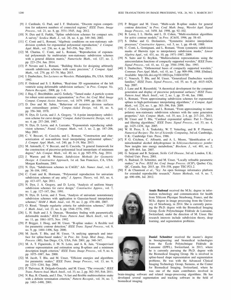
Anaïs Badoual received the M.Sc. degree in infor-mation technology and communication for healthfrom Télécom Physique Strasbourg, France, and theM.Sc. degree in image processing from the Univer-sity of Strasbourg, in 2014. She is currently pursu-ing the Ph.D. degree with the Biomedical ImagingGroup, École Polytechnique Fédérale de Lausanne,Switzerland, under the direction of M. Unser. Herresearch interests include subdivision theory, deeplearning, and segmentation problems.

Daniel Schmitter received the master’s degreein bioengineering and biomedical technologiesfrom the École Polytechnique Fédérale deLausanne (EPFL), Switzerland, in 2013, wherehe is currently pursuing the Ph.D. degree withthe Biomedical Imaging Group. He is involved inspline-based shape representation and segmentationproblems. He was with the Advanced ClinicalImaging Technology Group, Siemens, at the Centerfor Biomedical Imaging, Switzerland, where hewas one of the main contributors involved in

brain-imaging software and related image-processing algorithms. He hasdeveloped several segmentation and tracking software in the field ofbiomedical imaging.


Virginie Uhlmann received the M.Sc. degree in bio-engineering from the École Polytechnique Fédéralede Lausanne (EPFL), Switzerland, in 2012, whereshe is currently pursuing the Ph.D. degree withthe Biomedical Imaging Group, under the directionof M. Unser. She completed her master’s thesisin the Imaging Platform with the Broad Institute,Cambridge, MA, USA, under the supervision ofA. Carpenter. She is involved in applied problemrelated to image segmentation and tracking, andon approximation and spline theory. Her research

interests include image processing, computer vision, machine learning, andlife sciences.

She received the competitive Excellence Fellowship at the master’s levelfrom EPFL, in 2011 and 2012, and was awarded the Best Student PaperAward from the 2014 IEEE International Conference on Image Processing(ICIP’14). She also received a Best Student Paper Award nomination at theIEEE International Symposium on Biomedical Imaging in 2015.

Michael Unser (M’89–SM’94–F’99) was withthe Biomedical Engineering and InstrumentationProgram, National Institutes of Health, Bethesda,USA, conducting research on bioimaging, from1985 to 1997. He is currently a Professor andDirector of the Biomedical Imaging Group withthe École Polytechnique Fédérale de Lausanne,Switzerland. He has published over 250 journalpapers in his research fields. He is the author withP. Tafti of the book titled An Introduction to SparseStochastic Processes (Cambridge University Press,

2014). His primary area of investigation is biomedical image processing. Heis internationally recognized for his research contributions to sampling theory,wavelets, the use of splines for image processing, stochastic processes, andcomputational bioimaging.

Prof. Unser is an EURASIP Fellow (2009), and a member of the SwissAcademy of Engineering Sciences. He is the recipient of several internationalprizes, including three IEEE-SPS Best Paper Awards and two TechnicalAchievement Awards from the IEEE (2008 SPS and EMBS 2010). Hewas an Associate Editor-in-Chief (2003–2005) of the IEEE TRANSACTIONS

ON MEDICAL IMAGING. He is currently a member of the editorial boardsof the SIAM J. Imaging Sciences, the IEEE J. Selected Topics in SignalProcessing, and the Foundations and Trends in Signal Processing. He isthe Founding Chair of the Technical Committee on Bio Imaging and SignalProcessing (BISP) of the IEEE Signal Processing Society.

1188 ieee transactions on image processing, vol. 26, no. …big › publications ›...

Documents