1

12.1 Source: Foundations of Computer Science Cengage Learning

12

Abstract

Data Types

12.2

Define the concept of an abstract data type (ADT).

Define a stack, the basic operations on stacks, their applications

and how they can be implemented.

Define a queue, the basic operations on queues, their

applications and how they can be implemented.

Define a general linear list, the basic operations on lists, their

applications and how they can be implemented.

Define a general tree and its application.

Define a binary tree—a special kind of tree—and its

applications.

Define a binary search tree (BST) and its applications.

Define a graph and its applications.

Objectives After studying this chapter, the student should be able to:

2

12.3

12-1 BACKGROUND

Problem solving with a computer means processing data.

To process data, we need to define the data type and the

operation to be performed on the data. The definition

of the data type and the definition of the operation to be

applied to the data is part of the idea behind an abstract

data type (ADT) —to hide how the operation is

performed on the data. In other words, the user of an

ADT needs only to know that a set of operations are

available for the data type, but does not need to know

how they are applied.

12.4

Simple ADTs

Many programming languages already define some simple

ADTs as integral parts of the language. For example, the C

language defines a simple ADT as an integer. The type of

this ADT is an integer with predefined ranges. C also defines

several operations that can be applied to this data type

(addition, subtraction, multiplication, division and so on).

C explicitly defines these operations on integers and what we

expect as the results. A programmer who writes a C program

to add two integers should know about the integer ADT and

the operations that can be applied to it.

3

12.5

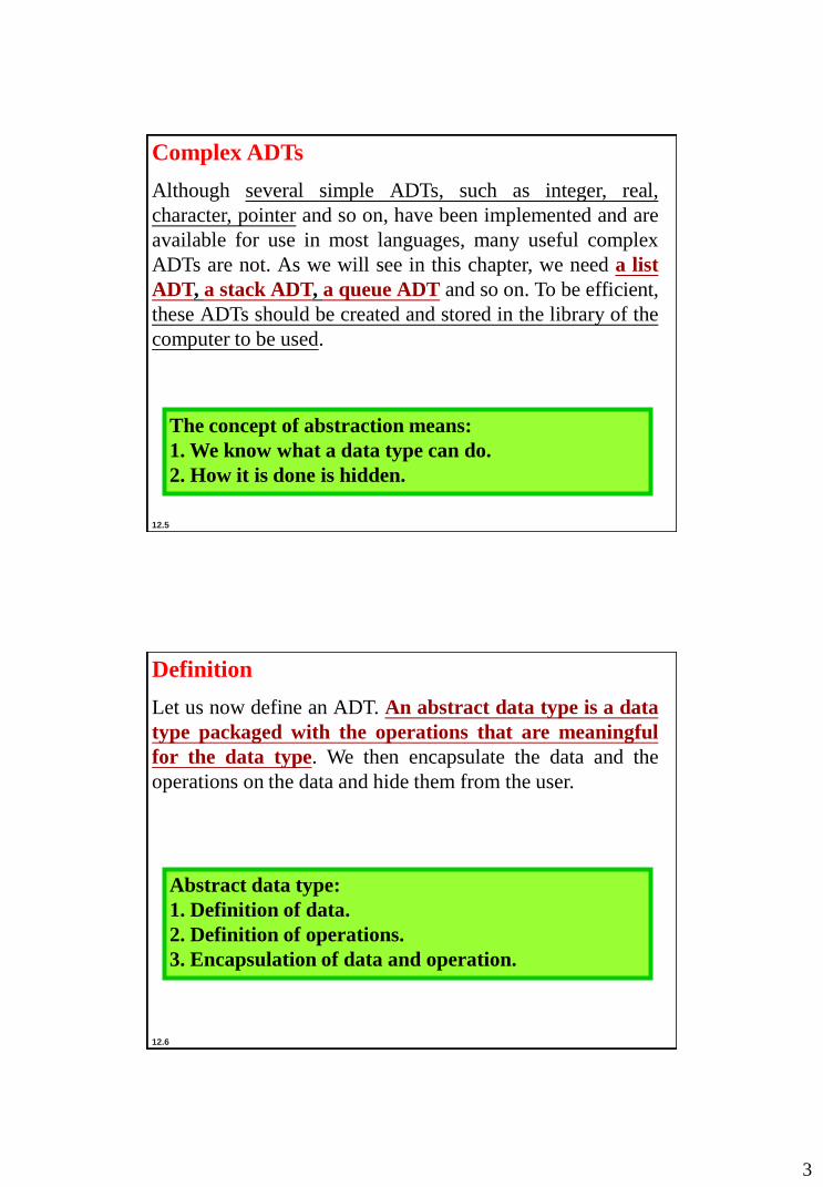
Complex ADTs

Although several simple ADTs, such as integer, real,

character, pointer and so on, have been implemented and are

available for use in most languages, many useful complex

ADTs are not. As we will see in this chapter, we need a list

ADT, a stack ADT, a queue ADT and so on. To be efficient,

these ADTs should be created and stored in the library of the

computer to be used.

The concept of abstraction means:

1. We know what a data type can do.

2. How it is done is hidden.

12.6

Definition

Let us now define an ADT. An abstract data type is a data

type packaged with the operations that are meaningful

for the data type. We then encapsulate the data and the

operations on the data and hide them from the user.

Abstract data type:

1. Definition of data.

2. Definition of operations.

3. Encapsulation of data and operation.

4

12.7

Model for an abstract data type

The ADT model is shown in Figure 12.1. Inside the ADT are

two different parts of the model: data structure and

operations (public and private).

Figure 12.1 The model for an ADT

12.8

Implementation

Computer languages do not provide complex ADT packages.

To create a complex ADT, it is first implemented and kept in

a library. The main purpose of this chapter is to introduce

some common user-defined ADTs and their applications.

However, we also give a brief discussion of each ADT

implementation for the interested reader. We offer the

pseudocode algorithms of the implementations as

challenging exercises.

5

12.9

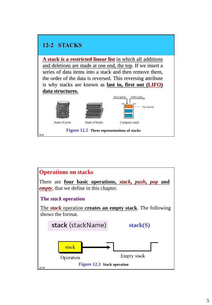
12-2 STACKS

A stack is a restricted linear list in which all additions

and deletions are made at one end, the top. If we insert a

series of data items into a stack and then remove them,

the order of the data is reversed. This reversing attribute

is why stacks are known as last in, first out (LIFO)

data structures.

Figure 12.2 Three representations of stacks

12.10

Operations on stacks

There are four basic operations, stack, push, pop and

empty, that we define in this chapter.

The stack operation

The stack operation creates an empty stack. The following

shows the format.

Figure 12.3 Stack operation

stack(S)

6

12.11

The push operation

The push operation inserts an item at the top of the stack.

The following shows the format.

Figure 12.4 Push operation

push(S,20)

push(S,78)

push(S,30) push (S,num)

{ top = top +1;

S[top] = num;

}

12.12

The pop operation

The pop operation deletes the item at the top of the stack.

The following shows the format.

Figure 12.5 Pop operation

pop(S,x); // x=30

pop (S)

{ num = S[top];

top = top -1;

return num;

}

7

12.13

The empty operation

The empty operation checks the status of the stack. The

following shows the format.

This operation returns true if the stack is empty and false if

the stack is not empty.

If empty(S)

12.14

Stack ADT

We define a stack as an ADT as shown below:

8

12.15

Give a stack S as below,

find Top = and S[top]= after Pop(S),

Push(S,25), Push(S,33), Pop(S), Pop(S), and Pop(S).

Top

3 4 5 6 7 8 9 1 2

43 68 92 14 28 75 56 S

12.16

Example 12.1

Figure 12.6 shows a segment of an algorithm that applies the

previously defined operations on a stack S.

Figure 12.6 Example 12.1

9

12.17

Stack applications

Stack applications can be classified into four broad

categories: reversing data, pairing data, postponing data

usage and backtracking steps. We discuss the first two in

the sections that follow.

Reversing data items

Reversing data items requires that a given set of data items

be reordered so that the first and last items are exchanged,

with all of the positions between the first and last also being

relatively exchanged.

For example,

the list (2, 4, 7, 1, 6, 8) becomes (8, 6, 1, 7, 4, 2).

12.18

Example 12.2

Convert a decimal integer to binary and print the results

10

12.19

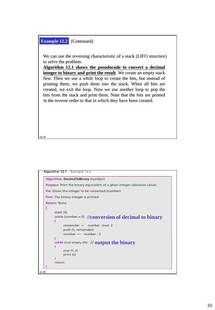
Example 12.2

We can use the reversing characteristic of a stack (LIFO structure)

to solve the problem.

Algorithm 12.1 shows the pseudocode to convert a decimal

integer to binary and print the result. We create an empty stack

first. Then we use a while loop to create the bits, but instead of

printing them, we push them into the stack. When all bits are

created, we exit the loop. Now we use another loop to pop the

bits from the stack and print them. Note that the bits are printed

in the reverse order to that in which they have been created.

(Continued)

12.20

//conversion of decimal to binary

// output the binary

11

12.21

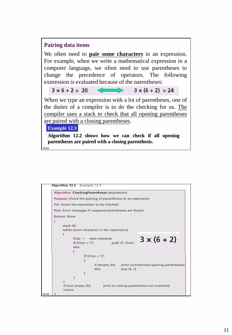
Pairing data items

We often need to pair some characters in an expression.

For example, when we write a mathematical expression in a

computer language, we often need to use parentheses to

change the precedence of operators. The following

expression is evaluated because of the parentheses:

When we type an expression with a lot of parentheses, one of

the duties of a compiler is to do the checking for us. The

compiler uses a stack to check that all opening parentheses

are paired with a closing parentheses.

Example 12.3

Algorithm 12.2 shows how we can check if all opening

parentheses are paired with a closing parenthesis.

12.22

12

12.23

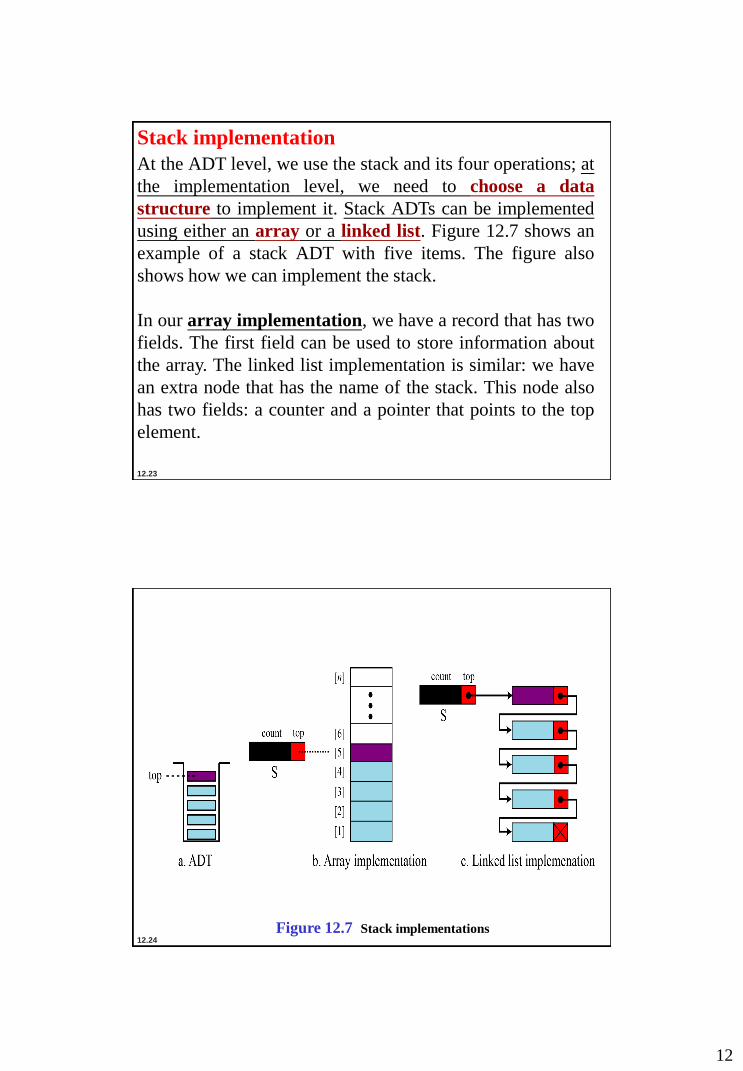
Stack implementation

At the ADT level, we use the stack and its four operations; at

the implementation level, we need to choose a data

structure to implement it. Stack ADTs can be implemented

using either an array or a linked list. Figure 12.7 shows an

example of a stack ADT with five items. The figure also

shows how we can implement the stack.

In our array implementation, we have a record that has two

fields. The first field can be used to store information about

the array. The linked list implementation is similar: we have

an extra node that has the name of the stack. This node also

has two fields: a counter and a pointer that points to the top

element.

12.24

Figure 12.7 Stack implementations

13

12.25

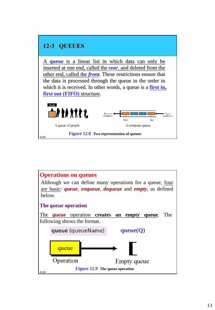
12-3 QUEUES

A queue is a linear list in which data can only be

inserted at one end, called the rear, and deleted from the

other end, called the front. These restrictions ensure that

the data is processed through the queue in the order in

which it is received. In other words, a queue is a first in,

first out (FIFO) structure.

Figure 12.8 Two representation of queues

12.26

Operations on queues

Although we can define many operations for a queue, four

are basic: queue, enqueue, dequeue and empty, as defined

below.

The queue operation

The queue operation creates an empty queue. The

following shows the format.

Figure 12.9 The queue operation

queue(Q)

14

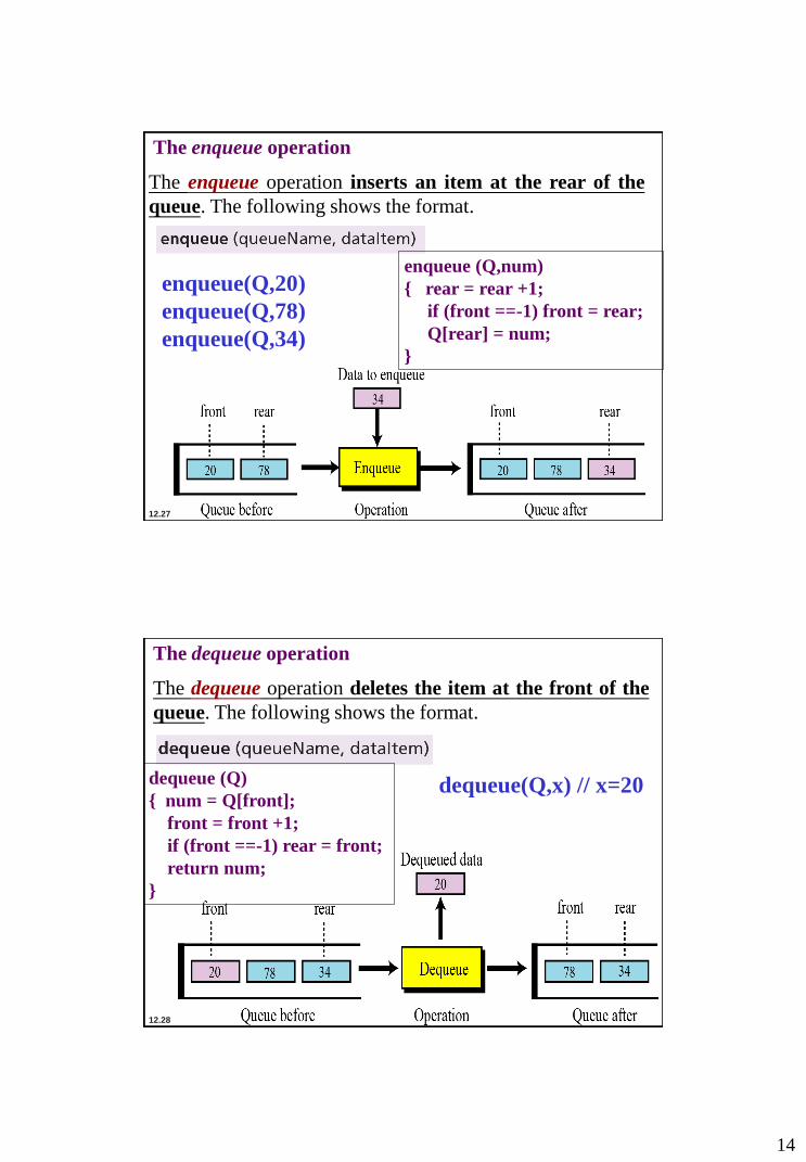
12.27

The enqueue operation

The enqueue operation inserts an item at the rear of the

queue. The following shows the format.

enqueue(Q,20)

enqueue(Q,78)

enqueue(Q,34)

enqueue (Q,num)

{ rear = rear +1;

if (front ==-1) front = rear;

Q[rear] = num;

}

12.28

The dequeue operation

The dequeue operation deletes the item at the front of the

queue. The following shows the format.

dequeue(Q,x) // x=20 dequeue (Q)

{ num = Q[front];

front = front +1;

if (front ==-1) rear = front;

return num;

}

15

12.29

The empty operation

The empty operation checks the status of the queue. The

following shows the format.

This operation returns true if the queue is empty and false if

the queue is not empty.

if empty(Q)

12.30

Queue ADT

We define a queue as an ADT as shown below:

16

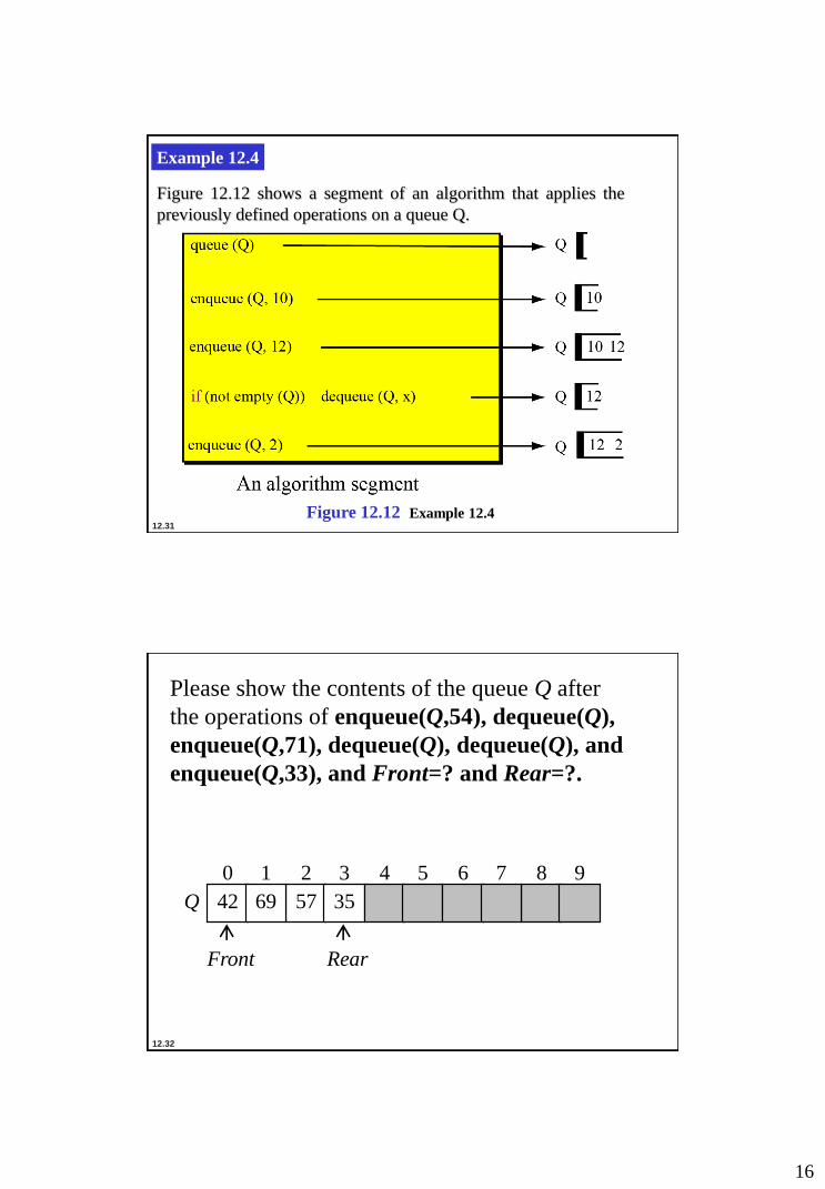
12.31

Example 12.4

Figure 12.12 shows a segment of an algorithm that applies the

previously defined operations on a queue Q.

Figure 12.12 Example 12.4

12.32

Please show the contents of the queue Q after

the operations of enqueue(Q,54), dequeue(Q),

enqueue(Q,71), dequeue(Q), dequeue(Q), and

enqueue(Q,33), and Front=? and Rear=?.

2 3 4 5 6 7 8 9 0 1

57 35 42 69 Q

Rear

Front

17

12.33

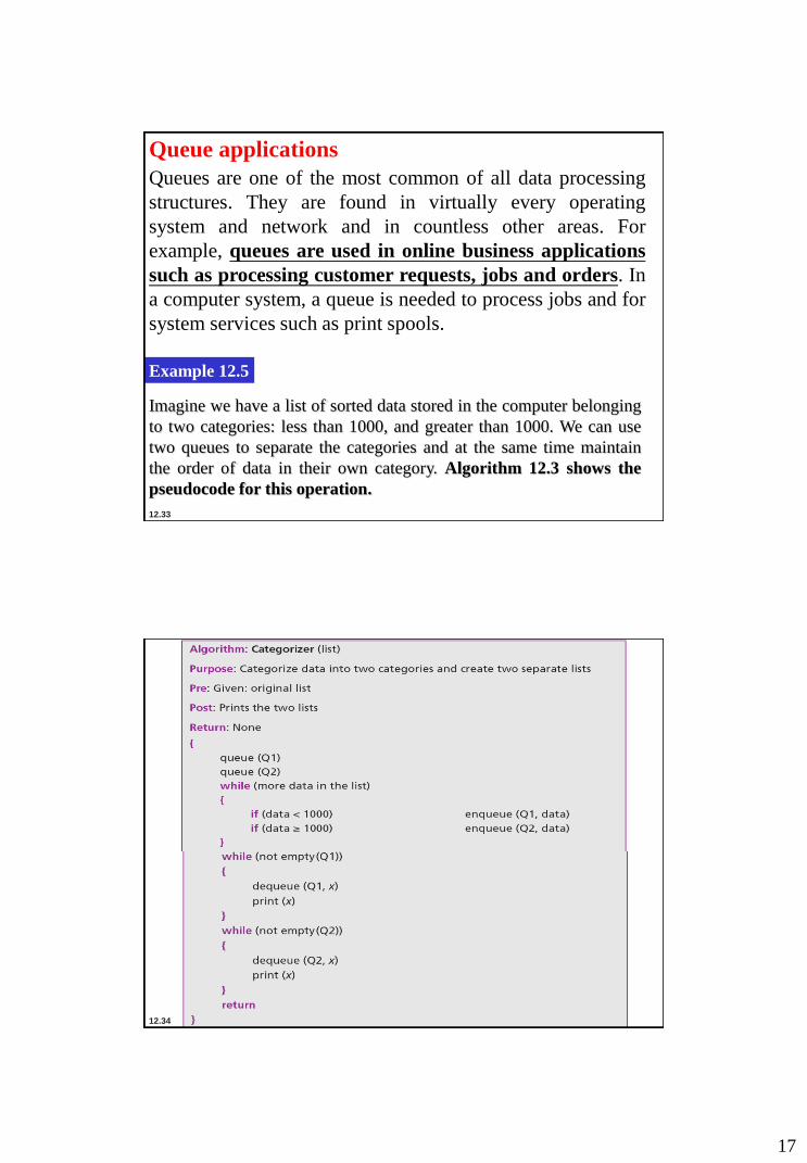
Queue applications

Queues are one of the most common of all data processing

structures. They are found in virtually every operating

system and network and in countless other areas. For

example, queues are used in online business applications

such as processing customer requests, jobs and orders. In

a computer system, a queue is needed to process jobs and for

system services such as print spools.

Example 12.5

Imagine we have a list of sorted data stored in the computer belonging

to two categories: less than 1000, and greater than 1000. We can use

two queues to separate the categories and at the same time maintain

the order of data in their own category. Algorithm 12.3 shows the

pseudocode for this operation.

12.34

18

12.35

Example 12.6

Another common application of a queue is to adjust and create

a balance between a fast producer of data and a slow

consumer of data. For example, assume that a CPU is connected

to a printer. The speed of a printer is not comparable with the

speed of a CPU. If the CPU waits for the printer to print some

data created by the CPU, the CPU would be idle for a long time.

The solution is a queue. The CPU creates as many chunks of data

as the queue can hold and sends them to the queue. The CPU is

now free to do other jobs. The chunks are dequeued slowly and

printed by the printer. The queue used for this purpose is

normally referred to as a spool queue.

12.36

Queue implementation

At the ADT level, we use the queue and its four operations at

the implementation level. We need to choose a data structure

to implement it. A queue ADT can be implemented using

either an array or a linked list. Figure 12.13 on page 329

shows an example of a queue ADT with five items. The

figure also shows how we can implement it. In the array

implementation we have a record with three fields. The first

field can be used to store information about the queue.

The linked list implementation is similar: we have an extra

node that has the name of the queue. This node also has three

fields: a count, a pointer that points to the front element and

a pointer that points to the rear element.

19

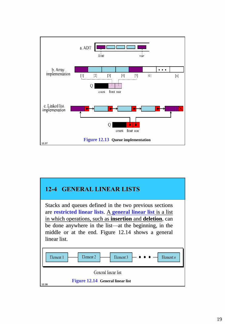
12.37

Figure 12.13 Queue implementation

12.38

12-4 GENERAL LINEAR LISTS

Stacks and queues defined in the two previous sections

are restricted linear lists. A general linear list is a list

in which operations, such as insertion and deletion, can

be done anywhere in the list—at the beginning, in the

middle or at the end. Figure 12.14 shows a general

linear list.

Figure 12.14 General linear list

20

12.39

Operations on general linear lists

Although we can define many operations on a general linear

list, we discuss only six common operations in this chapter:

list, insert, delete, retrieve, traverse and empty.

The list operation

The list operation creates an empty list. The following

shows the format:

12.40

The insert operation

Since we assume that data in a general linear list is sorted,

insertion must be done in such a way that the ordering of

the elements is maintained. To determine where the

element is to be placed, searching is needed. However,

searching is done at the implementation level, not at the ADT

level.

Figure 12.15 The insert operation

21

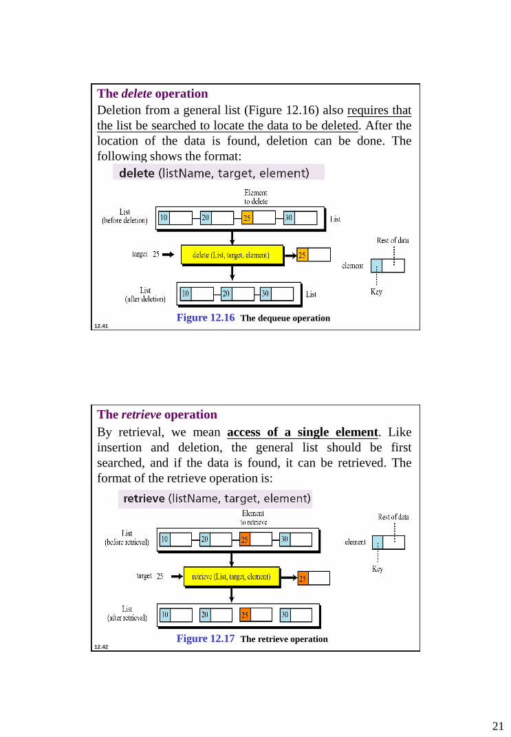
12.41

The delete operation

Deletion from a general list (Figure 12.16) also requires that

the list be searched to locate the data to be deleted. After the

location of the data is found, deletion can be done. The

following shows the format:

Figure 12.16 The dequeue operation

12.42

The retrieve operation

By retrieval, we mean access of a single element. Like

insertion and deletion, the general list should be first

searched, and if the data is found, it can be retrieved. The

format of the retrieve operation is:

Figure 12.17 The retrieve operation

22

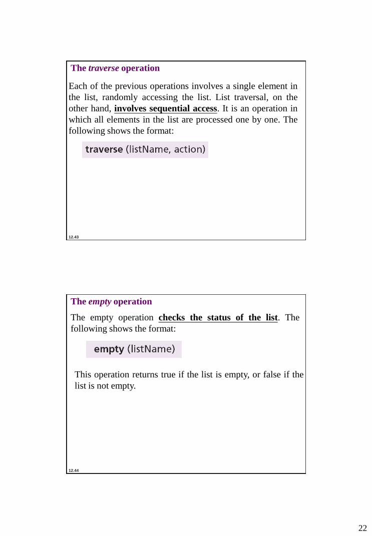
12.43

The traverse operation

Each of the previous operations involves a single element in

the list, randomly accessing the list. List traversal, on the

other hand, involves sequential access. It is an operation in

which all elements in the list are processed one by one. The

following shows the format:

12.44

The empty operation

The empty operation checks the status of the list. The

following shows the format:

This operation returns true if the list is empty, or false if the

list is not empty.

23

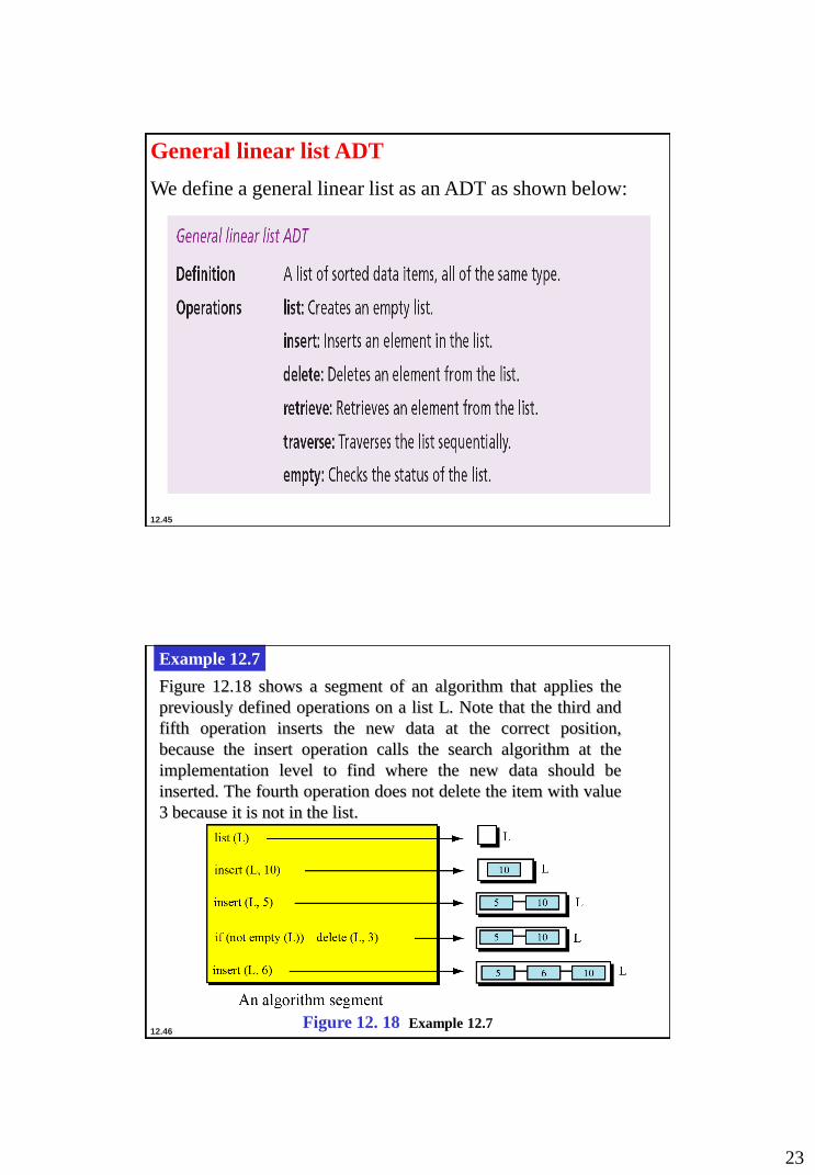
12.45

General linear list ADT

We define a general linear list as an ADT as shown below:

12.46

Example 12.7

Figure 12.18 shows a segment of an algorithm that applies the

previously defined operations on a list L. Note that the third and

fifth operation inserts the new data at the correct position,

because the insert operation calls the search algorithm at the

implementation level to find where the new data should be

inserted. The fourth operation does not delete the item with value

3 because it is not in the list.

Figure 12. 18 Example 12.7

24

12.47

General linear list applications

General linear lists are used in situations in which the

elements are accessed randomly or sequentially. For

example, in a college a linear list can be used to store

information about students who are enrolled in each

semester.

12.48

Example 12.8

A college has a general linear list that holds information about the

students and that each data element is a record with three fields: ID,

Name and Grade. Algorithm 12.4 shows an algorithm that helps a

professor to change the grade for a student. The delete operation

removes an element from the list, but makes it available to the program

to allow the grade to be changed. The insert operation inserts the

changed element back into the list. The element holds the whole record

for the student, and the target is the ID used to search the list.

25

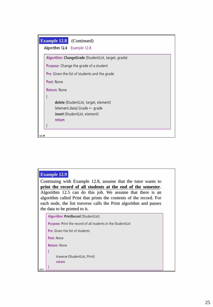
12.49

Example 12.8 (Continued)

12.50

Example 12.9

Continuing with Example 12.8, assume that the tutor wants to

print the record of all students at the end of the semester.

Algorithm 12.5 can do this job. We assume that there is an

algorithm called Print that prints the contents of the record. For

each node, the list traverse calls the Print algorithm and passes

the data to be printed to it.

26

12.51

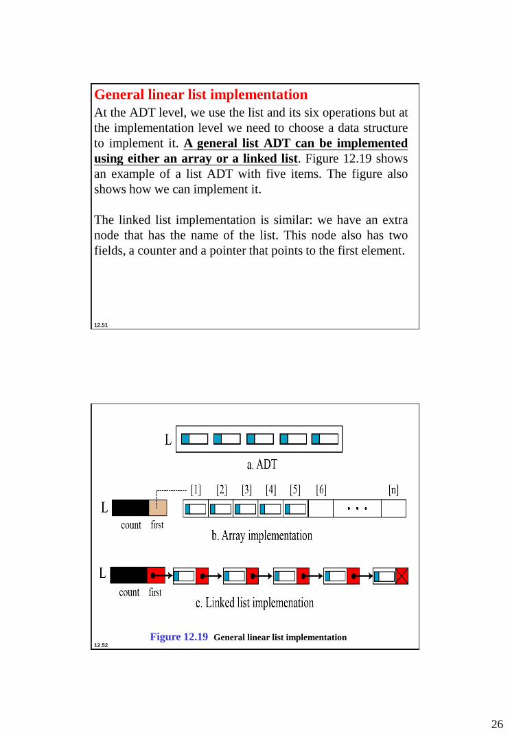
General linear list implementation

At the ADT level, we use the list and its six operations but at

the implementation level we need to choose a data structure

to implement it. A general list ADT can be implemented

using either an array or a linked list. Figure 12.19 shows

an example of a list ADT with five items. The figure also

shows how we can implement it.

The linked list implementation is similar: we have an extra

node that has the name of the list. This node also has two

fields, a counter and a pointer that points to the first element.

12.52

Figure 12.19 General linear list implementation

27

12.53

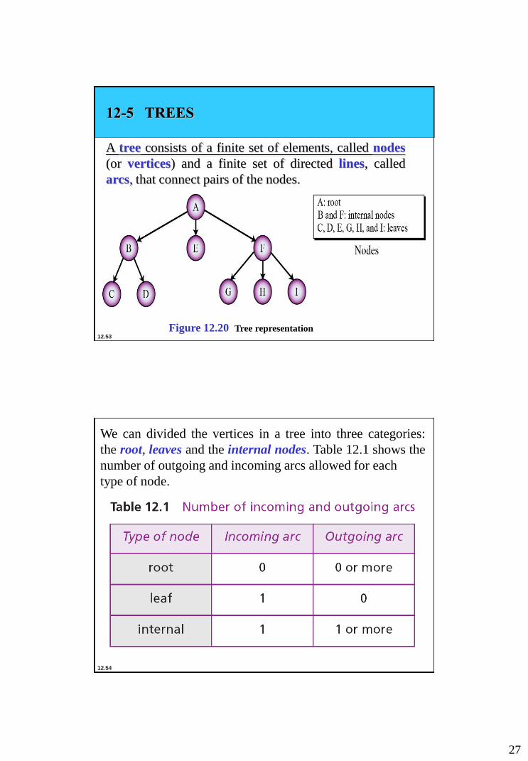
12-5 TREES

A tree consists of a finite set of elements, called nodes

(or vertices) and a finite set of directed lines, called

arcs, that connect pairs of the nodes.

Figure 12.20 Tree representation

12.54

We can divided the vertices in a tree into three categories:

the root, leaves and the internal nodes. Table 12.1 shows the

number of outgoing and incoming arcs allowed for each

type of node.

28

12.55

Each node in a tree may have a subtree. The subtree of each

node includes one of its children and all descendents of that

child. Figure 12.21 shows all subtrees for the tree in Figure

12.20.

Figure 12.21 Subtrees

12.56

Physical structure of a tree, each node includes one of its

children and all descendents of that child.

John

Mary Rom

Pat Ton Jessy

Root

29

12.57

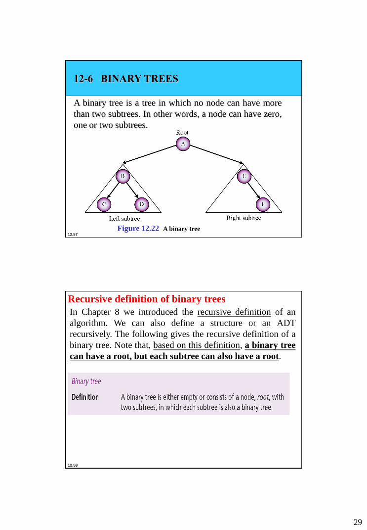
12-6 BINARY TREES

A binary tree is a tree in which no node can have more

than two subtrees. In other words, a node can have zero,

one or two subtrees.

Figure 12.22 A binary tree

12.58

Recursive definition of binary trees

In Chapter 8 we introduced the recursive definition of an

algorithm. We can also define a structure or an ADT

recursively. The following gives the recursive definition of a

binary tree. Note that, based on this definition, a binary tree

can have a root, but each subtree can also have a root.

30

12.59

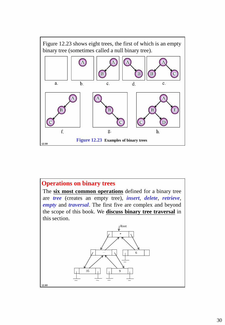
Figure 12.23 shows eight trees, the first of which is an empty

binary tree (sometimes called a null binary tree).

Figure 12.23 Examples of binary trees

12.60

Operations on binary trees

The six most common operations defined for a binary tree

are tree (creates an empty tree), insert, delete, retrieve,

empty and traversal. The first five are complex and beyond

the scope of this book. We discuss binary tree traversal in

this section.

*

－ 6

35 9

Root

31

12.61

Binary tree traversals

A binary tree traversal requires that each node of the tree

be processed once and only once in a predetermined

sequence. The two general approaches to the traversal

sequence are depth-first and breadth-first traversal.

Figure 12.24 Depth-first traversal of a binary tree

12.62

Example 12.10

Figure 12.25 shows how we visit each node in a tree using preorder

traversal. The figure also shows the walking order. In preorder

traversal we visit a node when we pass from its left side. The nodes

are visited in this order: A, B, C, D, E, F.

Figure 12.25 Example 12.10

32

12.63

Example 12.11

Figure 12.26 shows how we visit each node in a tree using breadth-

first traversal. The figure also shows the walking order. The traversal

order is A, B, E, C, D, F.

Figure 12.26 Example 12.11

12.64

Binary tree applications

Binary trees have many applications in computer science. In

this section we mention only two of them: Huffman coding

and expression trees.

Huffman coding

Huffman coding is a compression technique that uses

binary trees to generate a variable length binary code from

a string of symbols. We discuss Huffman coding in detail in

Chapter 15.

33

12.65

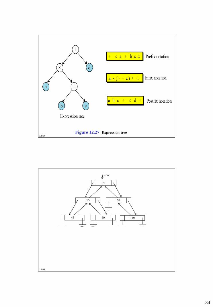
Expression trees

An arithmetic expression can be represented in three

different formats: infix, postfix and prefix. In an infix

notation, the operator comes between the two operands. In

postfix notation, the operator comes after its two operands,

and in prefix notation it comes before the two operands.

These formats are shown below for addition of two operands

A and B.

Prefix: +AB

Infix: A+B

Postfix: AB+

+

A B

Root

12.66

*

－ 6

35 9

Root

34

12.67

Figure 12.27 Expression tree

12.68

78

55 92

119 42 60

Root

35

12.69

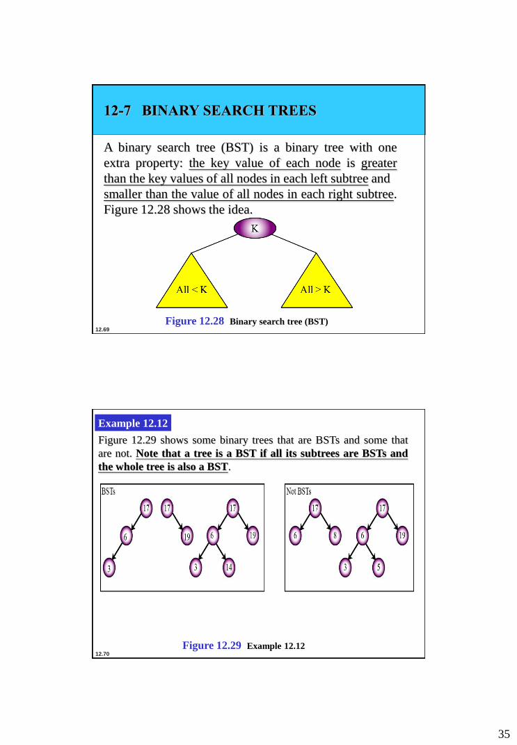
12-7 BINARY SEARCH TREES

A binary search tree (BST) is a binary tree with one

extra property: the key value of each node is greater

than the key values of all nodes in each left subtree and

smaller than the value of all nodes in each right subtree.

Figure 12.28 shows the idea.

Figure 12.28 Binary search tree (BST)

12.70

Example 12.12

Figure 12.29 shows some binary trees that are BSTs and some that

are not. Note that a tree is a BST if all its subtrees are BSTs and

the whole tree is also a BST.

Figure 12.29 Example 12.12

36

12.71

A very interesting property of a BST is that if we apply the

inorder traversal of a binary tree, the elements that are visited

are sorted in ascending order. For example, the three BSTs in

Figure 12.29, when traversed in order, give the lists

(3, 6, 17), (17, 19) and (3, 6, 14, 17, 19).

An inorder traversal of a BST creates a list that is

sorted in ascending order.

12.72

Another feature that makes a BST interesting is that we can

use a version of the binary search we used in Chapter 8 for a

binary search tree. Figure 12.30 shows the UML for a BST

search.

Figure 12.30 Inorder traversal of a binary search tree

37

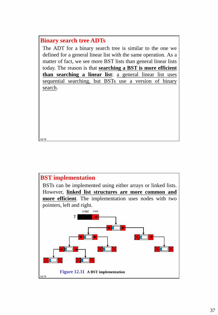
12.73

Binary search tree ADTs

The ADT for a binary search tree is similar to the one we

defined for a general linear list with the same operation. As a

matter of fact, we see more BST lists than general linear lists

today. The reason is that searching a BST is more efficient

than searching a linear list: a general linear list uses

sequential searching, but BSTs use a version of binary

search.

12.74

BST implementation

BSTs can be implemented using either arrays or linked lists.

However, linked list structures are more common and

more efficient. The implementation uses nodes with two

pointers, left and right.

Figure 12.31 A BST implementation

38

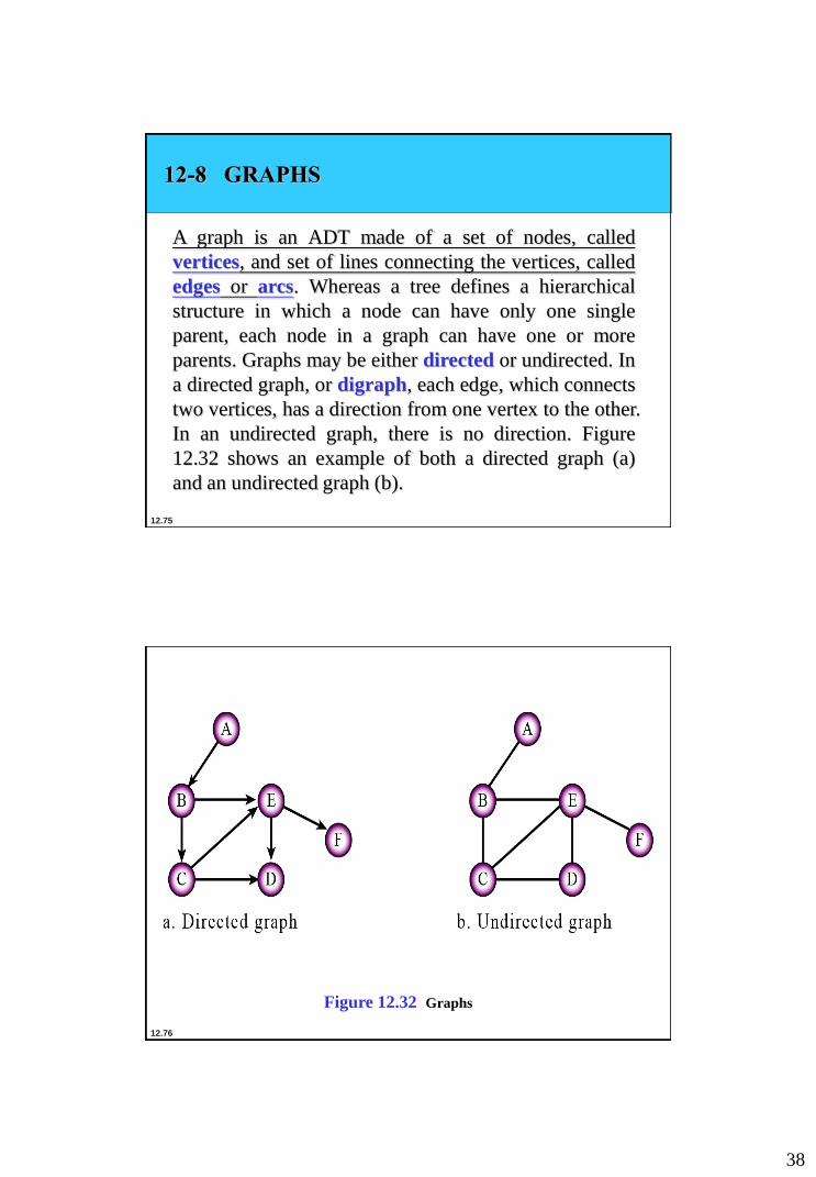
12.75

12-8 GRAPHS

A graph is an ADT made of a set of nodes, called

vertices, and set of lines connecting the vertices, called

edges or arcs. Whereas a tree defines a hierarchical

structure in which a node can have only one single

parent, each node in a graph can have one or more

parents. Graphs may be either directed or undirected. In

a directed graph, or digraph, each edge, which connects

two vertices, has a direction from one vertex to the other.

In an undirected graph, there is no direction. Figure

12.32 shows an example of both a directed graph (a)

and an undirected graph (b).

12.76

Figure 12.32 Graphs

39

12.77

Example 12.13

A map of cities and the roads connecting the cities can be

represented in a computer using an undirected graph. The cities

are vertices and the undirected edges are the roads that connect them.

If we want to show the distances between the cities, we can use

weighted graphs, in which each edge has a weight that represents

the distance between two cities connected by that edge.

Example 12.14

Another application of graphs is in computer networks (Chapter 6).

The vertices can represent the nodes or hubs, the edges can

represent the route. Each edge can have a weight that defines the

cost of reaching from one hub to an adjacent hub. A router can use

graph algorithms to find the shortest path between itself and the

final destination of a packet.