1234 transformation of general binary mrf … ieee transactions on pattern analysis and machine...

1234 IEEE TRANSACTIONS ON PATTERN ANALYSIS AND MACHINE INTELLIGENCE, VOL. 33, NO. 6, JUNE 2011

Transformation of General Binary MRFMinimization to the First-Order Case

Hiroshi Ishikawa, Member, IEEE

Abstract—We introduce a transformation of general higher-order Markov random field with binary labels into a first-order one thathas the same minima as the original. Moreover, we formalize a framework for approximately minimizing higher-order multilabel MRFenergies that combines the new reduction with the fusion-move and QPBO algorithms. While many computer vision problems todayare formulated as energy minimization problems, they have mostly been limited to using first-order energies, which consist of unaryand pairwise clique potentials, with a few exceptions that consider triples. This is because of the lack of efficient algorithms to optimizeenergies with higher-order interactions. Our algorithm challenges this restriction that limits the representational power of the models sothat higher-order energies can be used to capture the rich statistics of natural scenes. We also show that some minimization methodscan be considered special cases of the present framework, as well as comparing the new method experimentally with other suchtechniques.

Index Terms—Energy minimization, pseudo-Boolean function, higher order MRFs, graph cuts.

F

1 INTRODUCTION

M ANY problems in computer vision, such as segmenta-tion, stereo, and image restoration, are formulated as

optimization problems involving inference of the maximum aposteriori (MAP) solution of a Markov Random Field (MRF).Such optimization schemes have become quite popular, largelyowing to the success of optimization techniques such asgraph cuts [4], [10], [17], belief propagation [6], [25], andtree-reweighted message passing [16]. However, because ofthe lack of efficient algorithms to optimize energies withhigher-order interactions, most are represented in terms ofunary and pairwise clique potentials, with a few exceptionsthat consider triples [5], [17], [36]. This limitation severelyrestricts the representational power of the models: The richstatistics of natural scenes cannot be captured by such limitedpotentials [25]. Higher-order cliques can model more complexinteractions and reflect the natural statistics better. There arealso other reasons, such as enforcing connectivity [35] orhistogram [32] in segmentation, for the need of optimizinghigher-order energies.

This has long been realized [13], [27], [30], but with therecent success of the new energy optimization methods, thereis a renewed emphasis on the effort to find an efficientway to optimize MRFs of higher order. For instance, beliefpropagation variants [21], [28] have been introduced to doinference based on higher-order clique potentials. In graphcuts, Kolmogorov and Zabih [17] introduced a reduction thatcan reduce second-order binary-label potentials into pairwise

• The author is with the Department of Computer Science and Engineering,Waseda University, Tokyo 169-8555, Japan. E-mail: .

Manuscript received 25 Aug. 2009; revised 28 Dec. 2009; accepted 5 Mar.2010; published online 31 Mar. 2010.Recommended for acceptance by N. Paraqios.For information on obtaining reprints of this article, please send e-mail to:[email protected], and reference IEEECS Log NumberTPAMI-2009-08-0556.Digital Object Identifier no. 10.1109/TPAMI.2010.91.

ones, followed by an algebraic simplification by Freedmanand Drineas [7]. Kohli et al. [15], [14] extended the classof energies for which the optimal α-expansion and α-β -swap moves can be computed in polynomial time. Komodakisand Paragios [19] employed a master-slave decompositionframework to solve a dual relaxation to the MRF problem.Rother et al. [33] used a soft-pattern-based representation ofhigher-order functions that may for some energies lead tovery compact first-order functions with a small number ofnonsubmodular terms, as well as addressing the problem oftransforming general multilabel functions into quadratic ones.

In our approach, higher-order energies are approximatelyminimized by iterative “move-making,” in which higher-orderbinary energies are reduced to first-order ones and minimized.

Two recent advances in graph cuts made it possible. First,there is a generalization of the popular α-expansion algorithm[4] called the fusion move by Lempitsky et al. [22], [23].Second, a recent innovation allows optimization of first-ordernonsubmodular functions of binary variables. This method byBoros, Hammer, and their coworkers [1], [3], [8] is variouslycalled QPBO [18] or roof-duality [31]. This has a crucialimpact on the move-making algorithms since the choice ofthe move in each iteration depends on binary-label optimiza-tion. In the context of optimizing higher-order potentials, itmeans that some limitations that prevented the use of move-making algorithms for higher-order functions can possibly beovercome. As we mentioned, second-order potentials on binaryvariables can be reduced into pairwise ones [17]. However, therequirement that the result of reduction must be submodularmade its actual use quite rare. Thanks to the QPBO technique,now we can think of reducing higher-order potentials intopairwise ones, with a hope that at least part of the solutioncan be found. Woodford et al. [36] used this strategy verysuccessfully.

So far, the second-order case has remained the only casethat could be solved using this group of techniques because

0162–8828/11/$26.00 c⃝ 2011 IEEE Published by the IEEE Computer Society

ISHIKAWA: TRANSFORMATION OF GENERAL BINARY MARKOV RANDOM FIELD MINIMIZATION TO THE FIRST-ORDER CASE 1235

the reduction we mention above is only applicable in that case.To be sure, a totally different reduction technique that canreduce binary energies of any order has been known for a longtime [29]; however, to our knowledge it has never been usedsuccessfully in practice for orders higher than two. This seemsto be because, even though it can reduce any function into apairwise clique potential, the result is always nonsubmodularand hard to optimize in practice. We discuss it in Sections 3.2and 3.3, as well as experimentally investigating it in Section8.3.4.

In this paper, we introduce a new reduction techniquealong the lines of the Kolmogorov-Zabih reduction that canreduce any higher-order minimization problem of Markovrandom fields with binary labels into an equivalent first-orderproblem. Then, we combine it with fusion move and QPBOto approximately minimize higher-order multilabel energies.It also turns out that some of the known higher-order energyminimization techniques can be considered special cases of thenew framework. We demonstrate its effectiveness by testing iton a third-order potential, an image restoration problem thathas been used to test two BP algorithms [21], [28] capable ofoptimizing higher-order energies.

Part of this paper previously appeared as [11]. This extendedversion contains a new generalization of the reduction, discus-sions on the polynomial-time minimizability of the reducedenergy and necessary number of auxiliary variables, and aninvestigation of relations between the new algorithm and otherknown methods.

Organization of the Paper. In the next section, we providethe notation and definition for higher-order energy mini-mization. In Section 3, we briefly describe the two knownreductions of higher-order binary MRFs into first-order onesand discuss their limitations. In Section 4, we introduce thenew reduction in its simplest form. In Section 5, we generalizethe new reduction and discuss its various aspects. In Section 6,we describe the higher-order fusion-move algorithm using thenew reduction. In Section 7, we investigate the relations ofthe new method with other known methods. In Section 8,we report the results of our experiments. We conclude inSection 9.

2 PRELIMINARIES

In this section, we provide some notations and definitionspertinent to the areas of Markov random fields and higher-order energy minimization.

2.1 Markov Random Fields and Energy MinimizationProblemWe denote the set {0,1} of binary labels by B and the setof real numbers by R. The energy minimization problemconsidered here is as follows:

Let V be a set of pixels1 and L a set of labels, both finite sets.Also, let C be a set of subsets of V . We call an element of C a

1. Sometimes also called sites, they need not necessarily represent actualpixels, though they often do; consider it as just a name for the elements of afinite set.

clique. The cliques define a form of generalized neighborhoodstructure. In the case where all cliques consist of one or twopixels, it can be thought of as an undirected graph, where theset of cliques is divided into the set of all singleton subsetsand that of pairs, i.e., edges. In the general case, the pair (V,C)can be thought of as a hypergraph.

Let us denote by LV the set of labelings X : V → L, i.e.,assignments of a label Xv ∈ L to each pixel v∈V . In particular,the set of binary labelings is denoted by BV .

The energy E(X) is a real-valued function defined on thisset:

E : LV → R.

A crucial assumption is that E(X) is decomposable into asum

E(X) =∑C∈C

fC(XC), (1)

Here, for a clique C ∈ C, fC(XC) is a function that dependsonly on labels XC assigned by X to the pixels in C. We denotethe set of labelings on the clique C by LC; thus XC ∈ LC andfC : LC → R.

Supposing a random variable that takes values in L at eachpixel, the labeling X can be thought of as the system of randomvariables. Such a system, along with the energy, is called aMarkov random field (MRF).

The order of an MRF and its energy is defined to be thenumber of pixels in the largest clique minus one. Thus, anMRF of first order is of the form

E(X) =∑{v}∈C

f{v}(X{v})+∑

{u,v}∈C

f{u,v}(X{u,v}),

which is usually written as

E(X) =∑v∈V

fv(Xv)+∑

(u,v)∈E

fuv(Xu,Xv). (2)

Similarly, a second-order MRF can have cliques containingthree pixels and an energy of the form

E(X)=∑{v}∈C

f{v}(X{v})+∑

{u,v}∈C

f{u,v}(X{u,v})+∑

{u,v,w}∈C

f{u,v,w}(X{u,v,w}).

If we have a labeling X ∈ LV , we denote its restriction to asubset U ⊂V by X |U :

X |U ∈ LU , (X |U )v = Xv,v ∈U. (3)

2.2 Conditional Random FieldAn undirected graphical stochastic model that contains boththe hidden and the observed variables is sometimes calleda conditional random field (CRF) [20]. When the observedvariables are fixed, the rest of the model on the hiddenvariables is an MRF. The notion recently emerged from thearea of machine learning, where the observed data is often notfixed, and is instead used to learn the model itself.

In the vision literature, the term CRF is increasingly usedwhere the term MRF would have been used before, even wheresuch notions as learning are not used. Traditionally, MRFsused in the area tend to have the form where observed dataare associated with individual pixels, and the dependence of


the variable at a pixel on the observation only comes from thedata associated with that pixel. Perhaps because of this, theterm CRF is sometimes used to mean that a variable dependson the observed data associated with more than one pixel,even if the problem fixes the data at the beginning, making iteffectively an MRF problem.

In the context of energy minimization, the two terms MRFand CRF are used almost interchangeably since, at that levelwhere the optimization problem is already well-separatedfrom the context of stochastic modeling, there is no usefuldifference. One caveat, though, is that it can be confusingwhen the order of the random field is discussed. The order ofan MRF has long been defined as the number of the pixels inthe maximum clique in the energy minus one whereas, in thecase of the CRF, it is the same as the size of the maximumclique. Thus, a CRF of order k is an MRF of order k−1, whenthe observed variables are fixed.

2.3 Pseudo-Boolean FunctionsAn MRF energy that has labels in B is a function ofbinary variables: f : Bn → R, where n is the number ofpixels/variables. Such functions are called pseudo-Booleanfunctions (PBFs).

Any PBF can be uniquely represented as a polynomial ofthe form

f (x1, . . . ,xn) =∑S⊂V

cS∏i∈S

xi,

where V = {1, . . . ,n} and cS ∈ R. We refer the readers to [2],[9] for proof.

Combined with the definition of the order, this implies thatany binary-labeled MRF of order d−1 can be represented as apolynomial of degree d. Thus, the problem of reducing higher-order binary-labeled MRFs to first order is equivalent to that ofreducing general pseudo-Boolean functions to quadratic ones.

2.4 Minimization of PBFsA first-order binary energy (2) is said to be submodular if

fuv(0,0)+ fuv(1,1) ≤ fuv(0,1)+ fuv(1,0)

holds for every pairwise potential fuv for (u,v)∈E. First-orderbinary energies that are submodular can be minimized exactlyby an s-t-mincut algorithm [17]. The following well-knownproposition gives a convenient criterion for submodularitywhen the energy is given as a quadratic polynomial in binaryvariables:

Proposition 1. A quadratic pseudo-Boolean function

E(x1, . . . ,xn) =∑i, j

ai jxix j +∑

i

aixi +a

is submodular if and only if ai j ≤ 0 for all i, j.

Proof: The proposition follows directly from Proposition3.5 in Nemhauser et al. [26].

In this paper, we rely on the QPBO algorithm to minimizebinary-labeled energies. The algorithm returns a partial solu-tion assigning either 0 or 1 to some of the pixels, leaving

the rest unlabeled. Thus, if we run QPBO on a binary energyE(x) defined on BV , we obtain a partial labeling z∈BV ′

, whereV ′ ⊂V . The algorithm guarantees that the partial labeling is apart of a globally optimal one. That is, there exists a labelingy′ ∈BV that attains the global minimum and such that y′|V ′ = z.If the energy is submodular, QPBO labels all pixels, finding aglobal minimum.

Crucially for our purpose, QPBO has an “autarky” property[2], [3], [18]: If we take any labeling and “overwrite” it with apartial labeling obtained by QPBO, the energy for the resultinglabeling is not higher than that for the original labeling. Lety ∈BV be an arbitrary binary labeling and z ∈BV ′

the result ofrunning QPBO on an energy E(x), with V ′ ⊂V . Let us denoteby y▹ z ∈ BV the labeling obtained by overwriting y by z:

(y▹ z)v =

{zv, if v ∈V ′

yv, otherwise.(4)

Then, the autarky property means E(y▹ z) ≤ E(y).

3 KNOWN REDUCTIONS

There are a couple of known methods to reduce a higher-order function of binary variables to first-order one so thatthe minima of the reduced function can be translated easilyto those for the original function. Here, we outline the twoknown reduction methods and then discuss their limitations.

3.1 Reduction by Minimum SelectionKolmogorov and Zabih [17] first proposed this reduction inthe context of graph-cut optimization. Later, Freedman andDrineas [7] recast it into an algebraic formula.

Consider a cubic pseudo-Boolean function of x,y,z ∈ B

f (x,y,z) = axyz.

The reduction is based on the following identity:

xyz = maxw∈B

w(x+ y+ z−2). (5)

Let a < 0 be a real number. Then

axyz = minw∈B

aw(x+ y+ z−2).

Thus, whenever axyz appears in a minimization problem witha < 0, it can be replaced by aw(x+ y+ z−2).

If a > 0, we flip the variables (i.e., replace x by 1−x, y by1− y, and z by 1− z) of (5) and consider

(1− x)(1− y)(1− z) = maxw∈B

w(1− x+1− y+1− z−2).

This is simplified to

xyz = minw∈B

w(x+y+z−1)+(xy+yz+zx)−(x+y+z)+1. (6)

Therefore, if axyz appears in a minimization problem witha > 0, it can be replaced by

a{w(x+ y+ z−1)+(xy+ yz+ zx)− (x+ y+ z)+1}.

Thus, in either case, the cubic term can be replaced byquadratic terms. As we mentioned in Section 2.3, any binaryMRF of second order can be written as a cubic polynomial.


Then, each cubic monomial in the polynomial can be con-verted to a quadratic polynomial using one of the formulasabove, making the whole energy quadratic.

This reduction only works with cubic terms. For quarticterm axyzt, the same trick works if a < 0:

xyzt = maxw∈B

w(x+ y+ z+ t −3),

axyzt = minw∈B

aw(x+ y+ z+ t −3).

However, if a > 0,

(1− x)(1− y)(1− z)(1− t) = maxw∈B

w(−x− y− z− t +1)

becomes

xyzt = maxw∈B

w(−x− y− z− t +1)+(xyz+ xyt + xzt + yzt)

− (xy+ yz+ zx+ xt + yt + zt)+(x+ y+ z+ t)−1.

Unlike the cubic case, the maximization problem is not turnedinto a minimization. Similarly, this does not work with anyterm of even degree. This poses a severe restriction for whichfunction this reduction can be used in the case of degreeshigher than three.

In this paper, we remove this limitation in two ways. First,we introduce in Section 4 a new transformation that can beused for higher-degree terms with positive coefficients. In thequartic case, it gives:

xyzt = minw∈B

w(−2(x+y+z+t)+3)+xy+yz+zx+tx+ty+tz,

which expresses the quartic term as a minimum of a quadraticexpression, making it suitable for reduction of terms withpositive coefficients.

Also, we introduce in Section 5 a generalization of both theminimum selection and the new transformation that gives evenmore different ways of converting higher-order energies intofirst-order ones. This is accomplished by flipping some of thevariables before and after transforming the higher-order termto a minimum or maximum. For instance, another reductionfor the quartic term can be obtained using the technique: ifwe define x = 1− x, we have xyzt = (1− x)yzt = yzt − xyzt.The right-hand side consists of a cubic term and a quarticterm with a negative coefficient, which can be reduced usingthe minimum-selection technique (see equation (19) in Section5.4.) This generalization gives rise to an exponential number(in terms of occurrences of variables in the function) ofpossible reductions such that choosing which reduction touse is a whole new nontrivial problem. Although we cannotaddress the new problem thoroughly in this paper, we discusssome aspects of it in Section 5 and compare some specificreductions experimentally in Section 8.

3.2 Reduction by SubstitutionHowever, it has long since been known that the optimizationof pseudo-Boolean function of any degree can always be re-duced to an equivalent problem for quadratic pseudo-Booleanfunction. The method was proposed by Rosenberg [29] andhas since been recalled by Boros and Hammer [2].

In this reduction, the product xy of two variables x,y in thefunction is replaced by a new variable z, which is forced tohave the same value as xy at any minimum of the functionby adding penalty terms that would have a very large value ifthey do not have the same value.

More concretely, assume that x,y,z ∈ B and define

D(x,y,z) = xy−2xz−2yz+3z. (7)

Then, it is easy to check, by trying all eight possibilities, thatD(x,y,z) = 0 if xy = z and D(x,y,z) > 0 if xy = z. Consider anexample pseudo-Boolean function

f (x,y,w) = xyw+ xy+ y.

The reduction replaces xy by z and add MD(x,y,z):

f (x,y,w,z) = zw+ z+ y+MD(x,y,z), (8)

which has one more variable and is of one less degree than theoriginal function f . Here, M is chosen to be a large positivenumber so that, whenever xy = z and thus D(x,y,z) > 0, it isimpossible for f to take the minimum.

By repeating the above reduction, any higher-order func-tion can be reduced to a quadratic function with additionalvariables; for any minimum-energy value assignment for thenew function, the same assignment of values to the originalvariables gives the minimum energy to the original function.

3.3 The Problem with Reduction by Substitution

Reduction by substitution has not been used very often inpractice because, we suspect, it is difficult to make it work inpractice.

Note that, according to (7),

MD(x,y,z) = Mxy−2Mxz−2Myz+3Mz

in (8). The first term, Mxy, is a quadratic term with a verylarge positive coefficient, which in all cases makes the resultof the reduction nonsubmodular, according to Proposition 1.Though in using QPBO submodularity is not the only factor(see Section 5.2), it seems that such an energy cannot beminimized very well even with QPBO: in our experiments(Section 8.3) with this reduction, most variables were notassigned labels, leaving the move-making algorithm almostcompletely stalled.

4 THE NEW REDUCTION

In this section, we introduce a new reduction of higher-orderPBFs into quadratic ones. It is an extension of the reductionby minimum selection that we described in Section 3.1.

4.1 Quartic Case

Let us look at the quartic case. We would like to generalize (5)and (6) to higher degrees. Upon examination of these formulas,one notices that they are symmetric in the three variables x,y,and z. This suggests that any quadratic polynomial reduced


from xyzt should also be symmetric in the four variables.2

That is, if a generalized formula exists, it should look like

xyzt =minw

w(linear symmetric polynomial)

+(quadratic symmetric polynomial).

It is known that any symmetric polynomial can be written asa polynomial expression in the elementary symmetric polyno-mials. There is one elementary symmetric polynomial of eachdegree; the ones we need are:

s1 = x+ y+ z+ t,

s2 = xy+ yz+ zx+ tx+ ty+ tz.

Also, when the variables only take values in B, the squareof a variable is the same as itself. Thus, we have s1

2 = s1 +2s2, implying that any quadratic symmetric polynomial canbe written as a linear combination of s1,s2, and 1. Thus, theformula should be of the form:

xyzt = minw∈B

w(as1 +b)+ cs2 +ds1 + e.

An exhaustive search for integers a,b,c,d, and e that makesthe right-hand side positive only when x = y = z = t = 1 and0 otherwise yields:

xyzt = minw∈B

w(−2s1 +3)+ s2.

A similar search fails in finding a quintic formula, but increas-ing the number of auxiliary variables, we obtain:

xyztu = min(v,w)∈B2

{v(−2r1 +3)+w(−r1 +3)}+ r2,

where r1 and r2 are the first and second-degree elementarysymmetric polynomials in x,y,z, t, and u. In the same way,similar formulas for degrees six and seven can be found, fromwhich the general formula can be conjectured.

4.2 General CaseNow, we introduce similar reductions for general degree.Consider a monomial ax1 · · ·xd of degree d. We define theelementary symmetric polynomials in these variables as:

S1 =d∑

i=1

xi, S2 =d−1∑i=1

d∑j=i+1

xix j =S1(S1 −1)

2.

Case: a < 0. It is simple if a < 0:

ax1 · · ·xd = minw∈B

aw{S1 − (d −1)} , (9)

as given by Freedman and Drineas [7].

Case: a > 0. This case is our contribution:

ax1 · · ·xd = a minw1,...,wnd ∈B

nd∑i=1

wi(ci,d(−S1 +2i)−1

)+aS2,

(10)which follows from the following theorem:

2. Actually, the symmetry as a polynomial is not necessary. It has to besymmetric only on B4. See equation (19) in Section 5.4.

Theorem 1. For x1, . . . ,xd in B,

x1 · · ·xd = minw1,...,wnd ∈B

nd∑i=1

wi(ci,d(−S1 +2i)−1

)+S2, (11)

where

nd =⌊

d −12

⌋, ci,d =

{1, if d is odd and i = nd ,

2, otherwise.

Proof: Let us suppose that k of the d variables x1, . . . ,xdare 1 and the rest are 0. Then, it follows

S1 = k, S2 =k(k−1)

2.

Let us also define

l =⌊

k2

⌋, md =

⌊d −2

2

⌋, N = min(l,md),

A = minw1,...,wnd ∈B

md∑i=1

wi(−2S1 +4i−1)+S2.

Since the variables wi can take values independently,

A =md∑i=1

min(0,−2k +4i−1)+k(k−1)

2

If k is even (k = 2l), we have

−2k +4i−1 < 0 ⇐⇒ 4i < 4l +1 ⇐⇒ i ≤ l,

and if k is odd (k = 2l +1)

−2k +4i−1 < 0 ⇐⇒ 4i < 4l +3 ⇐⇒ i ≤ l.

Thus,

A =N∑

i=1

(−2k+4i−1)+k(k−1)

2= 2N2−N(2k−1)+

k(k−1)2

.

(12)We note that A = 0 if k ≤ d − 2. This can be seen by

checking the cases k = 2l and k = 2l + 1 in (12), noting thatl ≤ md and thus N = l.

Now, consider the even-degree case of (11). Since, in thatcase, nd = md and ci,d = 2, the right-hand side equals A. Thus,both sides are 0 if k ≤ d −2.

If k = d −1, A = 0 similarly follows from N = l = md .If k = d, then md = l −1. Thus, substituting N = l −1 and

k = 2l in (12), we have

A = 2(l −1)2 − (l −1)(4l −1)+ l(2l −1) = 1,

which completes the proof in the even-degree case.When d is odd, we have md = nd − 1 and the right-hand

side of (11) is

A+min(0,−S1 +2nd −1).

Since d = 2nd +1,

−S1 +2nd −1 ≥ 0 ⇐⇒ k ≤ d −2.

If k ≤ d −2, then A = 0 and −S1 +2nd −1 ≥ 0; thus, bothsides of (11) are 0.


If k = d −1, then

−S1 +2nd −1 = −k + k−1 = −1.

Also, since md = l − 1, using N = l − 1, k = 2l in (12), itfollows that

A = 2(l −1)2 − (l −1)(4l −1)+ l(2l −1) = 1,

showing that the both sides of (11) are 0.Finally, if k = d, we have

−S1 +2nd −1 = −k + k−1−1 = −2,

and from N = md = l −1,k = 2l +1, and (12),

A = 2(l −1)2 − (l −1)(4l +1)+ l(2l +1) = 3,

which shows that both sides of (11) are 1.Note that the cubic case of (11) is different from (6) and

simpler.As we mentioned above, any pseudo-Boolean function can

be written uniquely as a polynomial in binary variables. Sinceeach monomial in the polynomial can be reduced to a quadraticpolynomial using (9) or (10), depending on the sign of thecoefficient and the degree of the monomial, the whole functioncan be reduced to a quadratic polynomial that is equivalent tothe original function in the sense that, if any assignment ofvalues to the variables in the reduced polynomial achieves itsminimum, the assignment restricted to the original variablesachieves a minimum of the original function. Note that thereduction is valid whether the function is submodular or not.

5 GENERALIZATION AND RAMIFICATION

In this section, we introduce the “γ-flipped” version of thetransformation given in the previous section. By γ-flipping, weobtain many different reductions. So many, in fact, that anyserious comparison of different reductions, experimentally ortheoretically, will have to be left for future work. Comparinga few different reductions would not offer much information,as it would be akin to comparing the energy of a few labelingsin an MRF. Rather, we will need some algorithm or at leasta heuristic to guide the selection of which reduction to use.Nevertheless, we discuss some aspects of the transformationin this section, as well as testing the most obvious variantsexperimentally in Sections 8.3.3 and 8.3.5.

For b ∈ B, let us denote the negation of b, or 1−b, by b.When we allow the negations, the same PBF can be writtenin many different ways:

xyzt = (1− x)yzt = yzt − xyzt

= yzt − xzt + xyzt = zt − yzt − xzt + xyzt.

Let us call this manipulation flipping. By flipping some of thevariables before reducing to quadratic and then flipping themback after, we obtain many more reduction formulas.

An important caveat is that when the energy is minimized,variables x and x are not independent. Before using anyalgorithm, such as QPBO, that assumes independence of allvariables, we need to make sure that only one of x or x appearsin the energy for each variable x.

5.1 γ-Flipping Variables and FormulasThe monomial ax1 · · ·xd that we gave the reduction formulas(9) and (10) is a function that has a nonzero value onlywhen all the variables are 1. We generalize this to arbitrarycombinations of 0s and 1s.

For an arbitrary binary vector γ = (γ1, . . . ,γd) ∈ Bd , let usdefine

I0γ = {i |γi = 0}, I1

γ = {i |γi = 1}. (13)

Let x(γ) = (x(γ)1 , . . . ,x(γ)

d ) be a vector of variables defined fromγ and another vector x = (x1, . . . ,xd) of variables by

x(γ)i = γixi + γixi =

{xi, if γi = 1,

xi, if γi = 0.

We call x(γ) the γ-flipped version of the variable vector x.Then, the monomial ax(γ)

1 · · ·x(γ)d has a nonzero value a if and

only if x = γ:

ax(γ)1 · · ·x(γ)

d =

{a if x = γ,

0 otherwise.(14)

Let us define the γ-flipped elementary symmetric polyno-mials of degree one and two:

S(γ)1 =

d∑i=1

x(γ)i =

∑i∈I1

γ

xi +∑i∈I0

γ

(1− xi) = −d∑

i=1

(−1)γi xi +∣∣I0

γ∣∣ ,

S(γ)2 =

d−1∑i=1

d∑j=i+1

x(γ)i x(γ)

j =S(γ)

1 (S(γ)1 −1)2

.

Then the generalized reduction can be stated as follows:

Theorem 2. For x1, . . . ,xd in B, if a < 0,

ax(γ)1 · · ·x(γ)

d = minw∈B

aw{

S(γ)1 − (d −1)

}= min

w∈Baw

{−

d∑i=1

(−1)γi xi −∣∣I1

γ∣∣+1

}, (15)

and if a > 0

ax(γ)1 · · ·x(γ)

d = a minw1,...,wnd ∈B

nd∑i=1

wi

(ci,d(−S(γ)

1 +2i)−1)

+aS(γ)2 .

(16)

Proof: It directly follows from (9) or (10), depending onthe sign of a.

5.2 Polynomial-time Minimizability of the ReducedFunctionLooking at the generalized reduction (15) and (16) in viewof Proposition 1, we must conclude that there seems to be noobvious and general characterization for submodularity of theresulting quadratic polynomial.

In general, the right-hand side of (15) and (16) is not sub-modular. However, submodularity is not a necessary conditionfor the function to be globally minimizable in polynomial time.


For instance, flipping variables can make a nonsubmodularfunction into a submodular one.

The problem occurs when there is frustration, i.e., when itis not possible to consistently flip or not flip each variableso that coefficients of all quadratic terms are negative. Forinstance, we can make the coefficients of any two of the threequadratic terms negative in

xy+ yz+ zx = y− xy+ yz+ z− zx

= x− xy+ z− yz+ zx

= xy+ y− yz+ x− zx,

but not all three. If we only look at the term xy, we canmake it submodular in terms of variables x,y. But if thereare other occurrences of x in the energy as a whole, that maymake other terms nonsubmodular, as happens in the aboveexample. If the form of the clique potentials is such that thereis a way of flipping variables so that all quadratic monomialsbecome submodular, the energy would be globally minimiz-able in polynomial time using graph cuts, which happens inminimizing Pn Potts model with α-β -swap (Section 7.2.1.)

Guaranteed Cases. There are special forms of potentialsfor which we can guarantee that the reduced polynomial isminimizable in polynomial time using graph cuts.

The first case is when the term is of the form ax1 · · ·xd witha negative coefficients a, i.e., when γ = (1, . . . ,1) in (15). Thisfunction takes the value a when all of x1, . . . ,xd are 1, and 0otherwise. By the reduction, we have

ax1 · · ·xd = minw∈B

aw{S1 − (d −1)} ,

in which all of the quadratic monomials in awS1 have negativecoefficients, making it submodular according to Proposition 1.

Another case is the opposite, i.e., when the term is of theform ax1 · · · xd with a negative coefficient a, i.e., when γ =(0, . . . ,0) in (15). By the reduction, we have

ax1 · · · xd = minw∈B

aw{−S1 +1} ,

in which all of the quadratic monomials in −awS1 havepositive coefficients. This makes the potential supermodular.However, we can flip the auxiliary variable w so that thequadratic monomials in

−awS1 = minw∈B

(−a(1− w)S1)

have negative coefficients. This can be done without influenc-ing other parts of the energy since w appears nowhere else. Ifwe use the QPBO algorithm, this is automatically taken careof and no explicit flipping is necessary.

These two cases are hidden in the minimization of Pn Pottsmodel with α-expansion (Section 7.2.2).

5.3 γ-Flipped Representation of PBFsLet f : Bd →R be a pseudo-Boolean function. Then, from (14)it follows that

f (x) =∑γ∈Bd

f (γ)x(γ)1 · · ·x(γ)

d .

Moreover, for any λ ∈ R,

f (x) = λ +∑γ∈Bd

( f (γ)−λ )x(γ)1 · · ·x(γ)

d . (17)

In particular, by taking

λ = minγ∈Bd

f (γ),

we can make all of the coefficients in the sum (17) nonnega-tive. This is an example of the posiform representation of thePBF (See [2]).

Similarly, by taking

λ = maxγ∈Bd

f (γ), (18)

we can make all of the coefficients in (17) nonpositive. Thus,any PBF can be transformed to a quadratic PBF using only(15), by making all nonzero coefficients negative first. This isessentially what is done in the binary reduction by Rother etal. [33]. See Section 7.1 for more discussion.

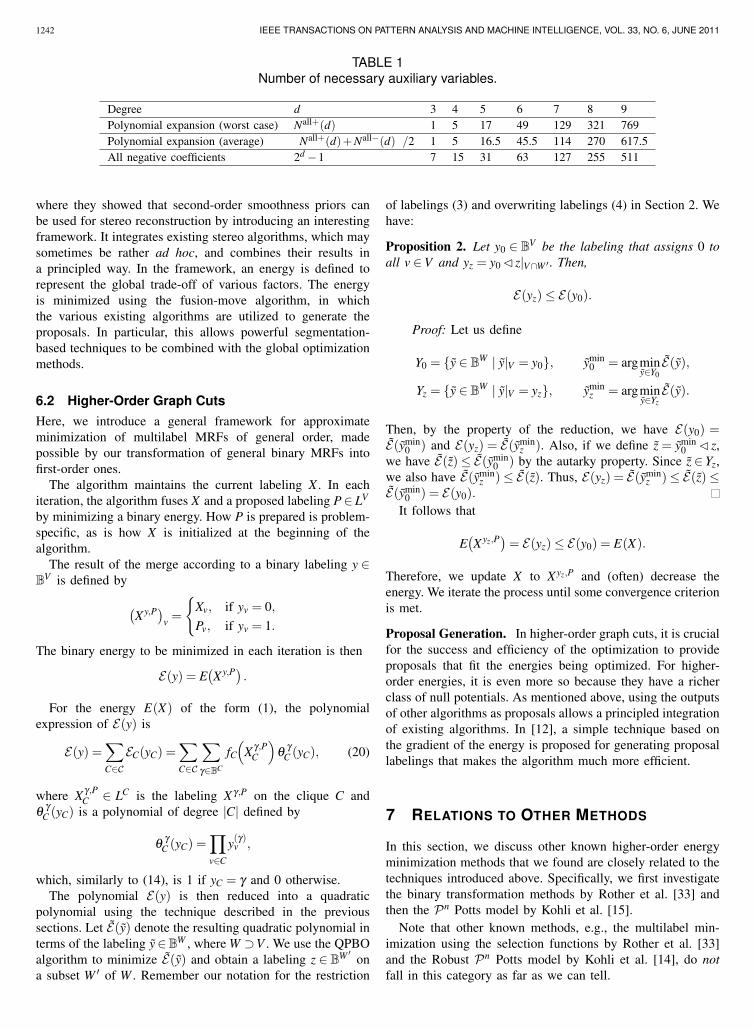
5.4 The Number of Necessary Auxiliary VariablesIn our reduction, the number of additional variables per cliquein the worst case is exponential in terms of the degree. Thisis because there are not only the highest-degree terms butalso lower-degree terms, each of which needs its own newvariables.

The exponential growth in the number of monomials in thegeneral case is in a sense unavoidable. Any PBF of d variablescan be represented as a polynomial of degree d, which has 2d

coefficients. For almost all such functions, all coefficients arenonzero. Since the reduction needs at least one variable foreach monomial with three or higher degree, the number ofextra variables must also increase exponentially as the orderof the energy increases.

As mentioned above, we can make one coefficient in thesum (17) zero and all other coefficients nonpositive by settingλ by (18). Since the transformation (15) in the negative caserequires only one new variable for converting each term, aminimization problem of any function of d binary variablescan be translated into the quadratic case by adding at most2d −1 auxiliary variables.

On the other hand, if we expand the function as a poly-nomial as in the previous section, there are at most

(di

)nonzero monomials of degree i. In the worst case, where eachmonomial has a positive coefficient, the number of auxiliaryvariables needed for using the transformation (10) is

Nall+(d) =d∑

i=3

(di

)⌊i−1

2

⌋= 2d−2(d −3)+1,

which is less than 2d − 1 when d ≤ 6. If the coefficients areall negative, the number is:

Nall−(d) =d∑

i=3

(di

)= 2d −1− d(d +1)

2,

which is the best case. In the average case, where one halfof the coefficients are negative and the other half positive, we


are better off in this respect using the polynomial expansionwhen d ≤ 7 (Table 1).

Note that in a clique potential, which generally wouldconsist of one or more monomials, each monomial can have adifferent mix of variables xi and their negations xi. Thus, forinstance, the monomial xyzt can be flipped and reduced:

minx,y,z,t∈B

xyzt = minx,y,z,t∈B

{−xyzt − yzt + zt}

= minx,y,z,t,u,w∈B

{−u(x+ y+ z+ t −3)−w(y+ z+ t −2)+ zt}

= minx,y,z,t,u,w∈B

{−u(−x+ y+ z+ t −2)−w(−y+ z+ t −1)+ zt} .

(19)

Although this particular example increases the number ofextra variables compared to simply using (10), in generalthe combination of variables and their negations to minimizethe number of auxiliary variables in the whole energy woulddepend on that particular energy.

Since there is an exponential number—not just in termsof the degree, but in terms of the number of occurrences ofthe variables in the whole energy—of possible combinations,finding the combination with the minimum number of neces-sary auxiliary variables seems a nontrivial problem. It may bean interesting direction for future research, especially if weallow an error tolerance for the energy value to deviate fromthe given exact value in favor of less auxiliary variables.

6 HIGHER-ORDER GRAPH CUTSTurning our attention to higher-order MRFs with more thantwo labels, in this section we formalize a framework forapproximately minimizing higher-order multilabel MRFs thatcombines the new reduction with the fusion-move and QPBOalgorithms.

6.1 Graph Cuts and Move-Making AlgorithmsCurrently, one of the most popular optimization techniquesin vision is α-expansion [4]. Here, we explain it and otheralgorithms to which the framework is directly related.

6.1.1 α-Expansion and α-β -SwapThe α-expansion and α-β -swap algorithms keep a currentlabeling and iteratively make a move, i.e., a change of labeling.In one iteration, the algorithms change the current labelingso that the energy becomes smaller or, at least, stays thesame. Such algorithms in general are called the move-makingalgorithms.

In the α-expansion algorithm, a label α ∈ L is chosen ateach iteration. The move is decided by either keeping theoriginal label or replacing it with α at each pixel. Thus,the “area” labeled α can only expand; hence the name α-expansion.

The choice of whether changing the label or not at eachpixel defines a binary labeling. The labeling after the movefrom X ∈ LV according to a binary labeling y ∈ BV is definedby:

(Xy,α)v =

{Xv, if yv = 0,

α , if yv = 1,

so that yv = 0 means that Xv stays the same and yv = 1 thatXv is changed to α .

An energy E(y) for the binary labeling y is defined byE(y) = E(Xy,α) as the multilabel energy after the move corre-sponding to binary labeling. By minimizing this binary energy,the move that reduces the energy most is chosen. When thebinary problem is submodular, it can be solved globally by ans-t mincut algorithm. By visiting all labels α in some orderand repeating it, E(X) is approximately minimized.

In the case of α-β -swap, allowed moves are defined as thosethat, at each pixel, keep the current label or swap the two fixedlabels α and β .

This was all done assuming that the energy E(X) is a first-order MRF. The algorithm has a guarantee on how close itcan approach the global minima in that case. Kohli et al.[15] investigated the case when E(X) is of higher order, andcharacterized the class of higher-order energies for which theglobally optimal α-expansion and α-β -swap moves can becomputed in polynomial time.

6.1.2 Fusion MovesThe fusion move [22], [23] is a simple generalization of α-expansion: in each iteration, define the binary problem as thepixelwise choice between two arbitrary labelings, instead ofbetween the current label and the fixed label α . Especiallyimportant to us is the variation where we maintain a currentlabeling X ∈ LV as in α-expansion and iteratively merge itwith a “proposal” labeling P ∈ LV by arbitrarily choosing oneof the two labelings to take the label from at each pixel.For instance, in the α-expansion algorithm, the proposal isa constant labeling that assigns the label α ∈ L to all pixels.Here, P can be any labeling.

It seems so simple and elegant that one may wonder whythe move-making algorithm was not formulated this way fromthe beginning. The answer is simple: it is because fusionmoves are nonsubmodular in general, whereas in the case ofα-expansion and α-β -swap moves, the submodularity can beguaranteed by some simple criteria. It is only because of theemergence of the QPBO/roof-duality optimization that we cannow consider the general fusion move.

6.1.3 Combining Fusion Moves and QPBOThe development of fusion moves and QPBO has an importantimplication in the optimization of higher-order energies. Aswe mentioned, the reduction in Section 3.1 has been knownfor some time. However, for the result of the reduction to beminimized with the popular techniques such as graph cuts, itmust be submodular. This requirement has kept its actual usequite rare. In combination with the QPBO algorithm, higher-order potentials may be approximately minimized by move-making algorithms. The derived binary energy, which wouldbe of the same order, can be reduced into pairwise one andthen at least a part of the solution may be found by QPBO,improving the current labeling iteratively. This is done bychanging the labels only at the nodes that were labeled byQPBO, which was proposed by Rother et al. [31].

The combination, which we might call the higher-ordergraph cuts, was first introduced by Woodford et al. [36],


TABLE 1Number of necessary auxiliary variables.

Degree d 3 4 5 6 7 8 9Polynomial expansion (worst case) Nall+(d) 1 5 17 49 129 321 769Polynomial expansion (average)

�Nall+(d)+Nall−(d)

�/2 1 5 16.5 45.5 114 270 617.5

All negative coefficients 2d −1 7 15 31 63 127 255 511

where they showed that second-order smoothness priors canbe used for stereo reconstruction by introducing an interestingframework. It integrates existing stereo algorithms, which maysometimes be rather ad hoc, and combines their results ina principled way. In the framework, an energy is defined torepresent the global trade-off of various factors. The energyis minimized using the fusion-move algorithm, in whichthe various existing algorithms are utilized to generate theproposals. In particular, this allows powerful segmentation-based techniques to be combined with the global optimizationmethods.

6.2 Higher-Order Graph CutsHere, we introduce a general framework for approximateminimization of multilabel MRFs of general order, madepossible by our transformation of general binary MRFs intofirst-order ones.

The algorithm maintains the current labeling X . In eachiteration, the algorithm fuses X and a proposed labeling P∈ LV

by minimizing a binary energy. How P is prepared is problem-specific, as is how X is initialized at the beginning of thealgorithm.

The result of the merge according to a binary labeling y ∈BV is defined by

(Xy,P)

v =

{Xv, if yv = 0,

Pv, if yv = 1.

The binary energy to be minimized in each iteration is then

E(y) = E(Xy,P) .

For the energy E(X) of the form (1), the polynomialexpression of E(y) is

E(y) =∑C∈C

EC(yC) =∑C∈C

∑γ∈BC

fC(

X γ,PC

)θ γ

C (yC), (20)

where X γ,PC ∈ LC is the labeling X γ ,P on the clique C and

θ γC (yC) is a polynomial of degree |C| defined by

θ γC (yC) =

∏v∈C

y(γ)v ,

which, similarly to (14), is 1 if yC = γ and 0 otherwise.The polynomial E(y) is then reduced into a quadratic

polynomial using the technique described in the previoussections. Let E(y) denote the resulting quadratic polynomial interms of the labeling y∈BW , where W ⊃V . We use the QPBOalgorithm to minimize E(y) and obtain a labeling z ∈ BW ′

ona subset W ′ of W . Remember our notation for the restriction

of labelings (3) and overwriting labelings (4) in Section 2. Wehave:

Proposition 2. Let y0 ∈ BV be the labeling that assigns 0 toall v ∈V and yz = y0 ▹ z|V∩W ′ . Then,

E(yz) ≤ E(y0).

Proof: Let us define

Y0 = {y ∈ BW | y|V = y0}, ymin0 = argmin

y∈Y0E(y),

Yz = {y ∈ BW | y|V = yz}, yminz = argmin

y∈YzE(y).

Then, by the property of the reduction, we have E(y0) =E(ymin

0 ) and E(yz) = E(yminz ). Also, if we define z = ymin

0 ▹ z,we have E(z) ≤ E(ymin

0 ) by the autarky property. Since z ∈Yz,we also have E(ymin

z ) ≤ E(z). Thus, E(yz) = E(yminz ) ≤ E(z) ≤

E(ymin0 ) = E(y0).

It follows that

E(Xyz,P

)= E(yz) ≤ E(y0) = E(X).

Therefore, we update X to Xyz,P and (often) decrease theenergy. We iterate the process until some convergence criterionis met.

Proposal Generation. In higher-order graph cuts, it is crucialfor the success and efficiency of the optimization to provideproposals that fit the energies being optimized. For higher-order energies, it is even more so because they have a richerclass of null potentials. As mentioned above, using the outputsof other algorithms as proposals allows a principled integrationof existing algorithms. In [12], a simple technique based onthe gradient of the energy is proposed for generating proposallabelings that makes the algorithm much more efficient.

7 RELATIONS TO OTHER METHODS

In this section, we discuss other known higher-order energyminimization methods that we found are closely related to thetechniques introduced above. Specifically, we first investigatethe binary transformation methods by Rother et al. [33] andthen the Pn Potts model by Kohli et al. [15].

Note that other known methods, e.g., the multilabel min-imization using the selection functions by Rother et al. [33]and the Robust Pn Potts model by Kohli et al. [14], do notfall in this category as far as we can tell.


7.1 Type-I and Type-II Transformation by Rother etal.

As we mentioned in Section 5.3, by taking

λ = maxγ∈Bd

f (γ),

we can make all nonzero coefficients in the sum (17) nonpos-itive. Thus, any PBF can be transformed to a quadratic PBFusing only the transformation (15), by making all coefficientsnonpositive first. It turns out that is essentially the same aswhat are called the Type-I and Type-II transformations inRother et al. [33].

Let θ > 0,γ ∈ Bd and define ψ(x) by:

ψ(x) =

{0, if x = γ,

θ , otherwise.

7.1.1 Type-I Transformation

Using (15), ψ(x) = θ −θx(γ)1 · · ·x(γ)

d is reduced to

ψ(x) = θ +θ minw∈B

w

{d∑

i=1

(−1)γi xi +∣∣I1

γ∣∣−1

}

= θ +θ minw∈B

w

∑i∈I0

γ

xi +∑i∈I1

γ

(1− xi)−1

= θ min

w∈B

1+ vw+(1− v)∑i∈I0

γ

xi +w

∑i∈I1

γ

(1− xi)−1

,

where we define v = w = 1−w. Note that vw = 0 and also thedefinition (13).

For x ∈ Bd ,v ∈ B, and w ∈ B, let us define

φ(x,v,w) = 1+ vw+(1− v)∑i∈I0

γ

xi +w

∑i∈I1

γ

(1− xi)−1

.

Then, we have

φ(x,0,0) = 1+∑i∈I0

γ

xi ≥ 1 = φ(x,1,0)

and

φ(x,1,1) = 1+∑i∈I1

γ

(1− xi) ≥ 1 = φ(x,1,0).

This implies that the minimum of φ(x,v,w) can always beachieved with v and w opposite. That is, having two variablesv and w does not improve the minimization; freeing themachieves at best the same minima as in the case when wefix v = w. Thus, we have

ψ(x) = θ minw∈B

φ(x, w,w) = θ minv,w∈B

φ(x,v,w).

The last expression is the same as what is called the Type-Itransformation in [33], which is given in the paper as:

ψ(x) =

minv,w∈B

θ

v+(1−w)− v(1−w)+∑i∈I0

γ

(1− v)xi +∑i∈I1

γ

w(1− xi)

.

7.1.2 Type-II TransformationIn [33], the Type-II transformation is defined as:

ψ(x) = θ +θ2

minw∈B

w(d −2)+w

∑i∈I1

γ

(1− xi)−∑i∈I0

γ

(1− xi)

+(1−w)

∑i∈I1

γ

xi −∑i∈I0

γ

xi

+∑i∈I0

γ

xi −∑i∈I1

γ

xi

,

which can be rewritten as

ψ(x) = θ +θ2

minw∈B

w

{d −2+

d∑i=1

(−1)γi (2xi −1)

}. (21)

Using (15), ψ(x) = θ −θx(γ)1 · · ·x(γ)

d can also be written as

ψ(x) = θ +θ minw∈B

w

{d∑

i=1

(−1)γi xi +∣∣I1

γ∣∣−1

}

= θ +θ2

minw∈B

w

{d∑

i=1

(−1)γi ·2xi +∣∣I1

γ∣∣+ (d −

∣∣I0γ∣∣)−2

}

= θ +θ2

minw∈B

w

{d∑

i=1

(−1)γi(2xi −1)+d −2

},

which coincides with (21).

To summarize, both Type-I and Type-II transformations in[33] are equivalent to (15), which is the γ-flipped version of thehigher-order transformation (9) based on those by Kolmogorovand Zabih [17] and Freedman and Drineas [7].

7.2 Pn Potts Model by Kohli et al.In [15], Kohli et al. define the class of the following form ofclique potential and call it the Pn Potts model:

fC(XC) =

{νl , if Xv = l for all v ∈C,

νmax, otherwise,(22)

where νl ∈ R is defined for each l ∈ L so that νmax ≥ νl .We consider minimizing the energy (1) with the higher-

order clique potential (22), using the higher-order graph-cutalgorithm in Section 6, where the proposals emulate α-β -swapand α-expansion. In the following, we ignore the constant andlinear energy terms.


7.2.1 α-β -SwapThe α-β -swap algorithm can be emulated as follows. Assumethat we are in an iteration in the algorithm with the currentlabeling X ∈ LV and let α,β ∈ L,α = β . Let us denote

Cl = {v ∈C |Xv = l}, for l ∈ L,

Cγ = {v ∈C |γv = 1}, Cγ = {v ∈C |γv = 0}.

We define the proposal labeling by

Pv =

α, if v ∈Cβ ,

β , if v ∈Cα ,

Xv, otherwise.

Let us consider the binary clique potential fC(

X γ,PC

)for

clique C and binary labeling γ ∈ BC.1. If Cα ∪Cβ = C,

fC(

X γ,PC

)=

να , if Cγ = Cα and Cγ = Cβ ,

νβ , if Cγ = Cα and Cγ = Cβ ,

νmax, otherwise.

2. If C = Cl , where l = α, l = β , then

fC(

X γ,PC

)= νl ,

since Pv = Xv = l for all v ∈C.3. Otherwise, there is no way the whole clique would have

the same label after an α-β -swap. Hence,

fC(

X γ,PC

)= νmax.

Remember the PBF E(y) in (20). We only have to considerthe nonconstant case 1), when

EC(yC) = νmax +δα∏

v∈Cα

yv∏

v∈Cβ

yv +δβ∏

v∈Cα

yv∏

v∈Cβ

yv,

where δα = να −νmax and δβ = νβ −νmax.Since δα ≤ 0 and δβ ≤ 0, the energy can be reduced by (15)

as

δα∏

v∈Cα

yv∏

v∈Cβ

yv = minuC∈B

δα uC

1−|Cβ |−∑v∈Cα

yv +∑v∈Cβ

yv

,

(23)

δβ∏

v∈Cα

yv∏

v∈Cβ

yv = minwC∈B

δβ wC

1−|Cα |+∑v∈Cα

yv −∑v∈Cβ

yv

.

(24)

The transformation adds new variables up to twice the numberof cliques. In practice, many cliques would be in cases 2)or 3) above and have the constant νl or νmax as their binaryclique potential, reducing the number of variables in the binaryminimization problem.

Unless C = Cα or C = Cβ , neither (23) nor (24) falls in thespecial cases that allow polynomial-time global minimization,which we discussed in Section 5.2. However, for this particularenergy, we can systematically flip variables so that the wholeenergy becomes globally optimizable. For instance, we can flip

all variables in Cβ , i.e., consider yv as the variable instead ofyv for all v ∈V such that Xv = β . Then, the same variables areflipped regardless of which clique they appear in. The energythen becomes

EC(yC) = νmax + minuC∈B

δα uC

1−∑v∈Cα

yv −∑v∈Cβ

yv

+ min

wC∈Bδβ wC

1−|C|+∑v∈Cα

yv +∑v∈Cβ

yv

,

and, as we discussed in Section 5.2, this form of energy canbe globally minimized with graph cuts.

7.2.2 α-ExpansionLet us next consider using the proposal emulating α-expansion, i.e.,

Pv = α for all v ∈V,

where α ∈ L. Let us also denote

Cα = {v ∈C |Xv = α}.

Assume that we are in an iteration in the algorithm, withcurrent labeling X ∈ LV . Then the clique potential for thebinary labeling γ ∈ BC would be:

fC(

X γ,PC

)=

ν , if γv = 0 for all v ∈C,

να , if γv = 1 for all v ∈Cα ,

νmax, otherwise,

where ν depends on the current labeling XC on the clique C:

ν =

{νl , if Xv = l for all v ∈C,

νmax, otherwise.

Let us define δ = ν − νmax and δα = να − νmax. Thepotential function EC(yC) in (20) would be:

EC(yC) = νmax +δ∏v∈C

yv +δα∏

v∈Cα

yv.

Since δ ≤ 0 and δα ≤ 0, the energy can be reduced by (15) as

δ∏v∈C

yv = minuC∈B

δuC

(1−∑v∈C

yv

), (25)

δα∏v∈C

yv = minwC∈B

δα wC

∑v∈Cα

yv +1−|Cα |

. (26)

Thus, the transformation adds new variables twice the numberof cliques. In practice, the (25) part in E(y) vanishes for allbut those cliques where the current labeling assigns the samelabel to all of the pixels in the clique.

Note also that (25) and (26) are the two special cases wediscussed in Section 5.2 that allow polynomial-time globalminimization.

Thus, we have reproduced the results described in Kohli etal. [15], Section 4.3. That is, in optimizing the Pn Potts model(22) with α-β -swap and α-expansion, the binary energy ineach iteration can be solved globally using graph cuts.


8 EXPERIMENTS

As we discussed above, the Pn Potts model can be minimizedusing the higher-order graph cuts. Moreover, since the con-struction in Kohli et al. [15] and our algorithm both minimizethe binary energy exactly, the results should be the same,except for the rare cases where there is more than one globalminima. Since their experiments in texture-based segmentationuses the Pn Potts model, we can expect almost exactly thesame results if we used the same energy in our algorithm.

Here, we report the results of comparing with other al-gorithms. The higher-order BP variants by Lan et al. [21]and Potetz [28] were both tested using a particular higher-order image restoration problem. We use the same problemto compare the effectiveness of the higher-order graph-cutalgorithm with them.

8.1 Image Denoising with Fields of Experts

The image restoration scheme uses the recent image statisticalmodel called the Fields of Experts (FoE) [30], which capturescomplex natural image statistics beyond pairwise interactionsby providing a way to learn an image model from naturalscenes. FoE has been shown to be highly effective, performingwell at image denoising and image inpainting using a gradientdescent algorithm.

The FoE model represents the prior probability of an imageX as the product of several Student’s t-distributions:

p(X) ∝∏C

K∏i=1

(1+

12(Ji ·XC)2

)−αi

, (27)

where C runs over the set of all n×n patches in the image, andJi is an n×n filter. The parameters Ji and αi are learned from adatabase of natural images. In both [21] and [28], 2×2 patcheswere used to show that 2 × 2 FoE improves over pairwisemodels significantly.

We are given the noisy image N ∈ LV and find the maximuma posteriori solution given the prior model (27). The prior givesrise to a third-order MRF, with clique potentials that dependon up to four pixels. Since the purpose of the experimentsis not the image restoration per se, but a comparison ofthe optimization algorithms, we use exactly the same simplemodel as in the two predecessors.

It is an inference problem with a simple likelihood term:image denoising with a known additive noise. We assumethat the images have been contaminated with an i. i. d.Gaussian noise that has a known standard deviation σ . Thus,the likelihood of noisy image N given the true image X isassumed to satisfy

p(N|X) ∝∏v∈V

exp(− (Nv −Xv)2

2σ2

). (28)

To maximize the a posteriori probability p(X |N) given thenoisy image N, we have to maximize p(N|X)p(X), the productof the likelihood and the prior probability.

8.2 Minimization Algorithm

We use the higher-order graph-cut algorithm described inSection 6 with the following ingredients.

Initialization. We initialize X by N, the given noisy image.

Convergence Criterion. We iterate until the energy decreaseover 20 iterations drops below a convergence threshold θc. Weused the values θc = 8 for σ = 10 and θc = 100 for σ = 20.

Proposal Generation. For proposal P, we use the followingtwo in alternating iterations:1. A uniform random image created each iteration.2. A blurred image, which is made every 30 iterations by

blurring the current image X with a Gaussian kernel (σ =0.5625).

For comparison, we also test the α-expansion proposal, i.e., aconstant image that gives the same value α everywhere.

Cliques. We consider the set C of cliques C = C1∪C4, whereC1 = {{v}|v ∈V} is the set of singleton cliques and C4 is theset of all 2×2 patches in the image.

Energy. The local energy fC(XC) in (1) is defined by

f{v}(X{v}) =(Nv −Xv)2

2σ2 , ({v} ∈ C1)

fC(XC) =K∑

i=1

αi log(

1+12(Ji ·XC)2

). (C ∈ C4)

These are negative logarithm of the clique potentials in thelikelihood (28) and the prior (27), respectively. Minimizingthis energy is the same as maximizing the a posteriori prob-ability p(X |N) given the data N.

QPBO. For the QPBO algorithm, we used the C++ codemade publicly available by Vladimir Kolmogorov. We alsoused the variations of QPBO included in the code.

8.3 Results

8.3.1 Qualitative DifferenceFig. 1 shows the qualitative difference between the denoisingresults using first-order and third-order energies. Images inFigs. 1a and 1b show the original image and the image withnoise added at σ = 20, respectively. All images in this figureare 160× 240-pixel 8-bit grayscale images. Images in Figs.1c and 1d show the result of denoising using α-expansion byfirst-order energy

E(X) =∑v∈V

(Nv −Xv)2 +λ

∑(u,v)

Potts(Xu,Xv), (29)

where the pairwise Potts potential is defined for vertical andhorizontal neighbors u,v ∈V so that Potts(Xu,Xv) is 1 if Xu =Xv and 0 otherwise; and λ = 250 for Fig. 1c and λ = 400 forFig. 1d. The image in Fig. 1e shows the result of denoisingby first-order total-variation energy:

E(X) =∑v∈V

(Nv −Xv)2 +λ

∑(u,v)

|Xu −Xv|. (30)


The energy was globally minimized using the technique in [10]with λ = 10. Finally, the image in Fig. 1f shows the result ofdenoising by the FoE energy described above.

The Potts model favors piecewise-constant images, whichcan be clearly seen in the results. If λ is small, much noiseremains, as in Fig. 1c. If we make λ larger, the result becomestoo flat, as in Fig. 1d. The total variation does a better job (asin Fig. 1e), but the same dilemma as with the Potts model stillremains. The result (as in Fig. 1f) by the third-order energyclearly is the best qualitatively.

Some more denoising examples are shown in Fig. 2.

8.3.2 Quantitative Comparison

For quantitative comparison, we measured the mean energyand the mean peak signal-to-noise ratio (PSNR) for denoisingresults over the same set of 10 images that were also usedin both [21] and [28]. The images are from the Berkeleysegmentation database [24], grayscaled and reduced in size,as well as with the added Gaussian noise with σ = 10,20.Here, PSNR = 20log10(255/

√MSE), where MSE is the mean

squared error. The test images and the FoE model were kindlyprovided by Stefan Roth, one of the authors of [21], [30]. BrianPotetz also obliged by providing us with his results.

The PSNR and energy numbers are listed in Table 2. Forcomparison, we also included the result by simple gradientdescent by [30]. The energy results show that the higher-ordergraph cuts using the third-order energy outperforms the bothBP variants optimizing the same energy. The PSNR is alsocomparable to [28] and better than [21]. Our algorithm takes6-10 minutes (250−280 iterations) to converge on a 2.93 GHzXeon E5570 processor. By comparison, according to [28], ittook 30-60 minutes on a 2.2 GHz Opteron 275, while thealgorithm in [21] takes 8 hours on a 3 GHz Xeon. Thus,our algorithm outperforms the two predecessors in qualityand speed, though BP is considered to be substantially moreparallelizable than graph cuts.

8.3.3 Comparison by Reductions, Proposals, andQPBO Variations

Fig. 3 shows the behavior of some numbers during theoptimization when σ = 20. The three graphs show energy,PSNR, and the ratio of pixels that is labeled by QPBO.

First, compare the solid dark-red diamonds and the solidpurple squares. They represent the two ways of handlingpositive-coefficient terms in binary energy reduction, bothusing the blur and random proposal and the QPBO algorithm.Shown as the dark-red diamonds, using (11) in Theorem1 is a little slower in this particular case. Flipping onevariable in a positive-coefficient term before reducing it bythe Kolmogorov-Zabih technique and then flipping the variableback (see, for example, (19)) yields the purple square plot. Itis a little faster, due to the higher ratio of pixels labeled bythe QPBO algorithm, although it uses more memory because itneeds more (about 4.4 percent in this case) auxiliary variables.

Next, compare the two dark-red plots marked by hollow andsolid diamonds in each graph. These compare the blur andrandom proposal (solid diamond) and α-expansion proposal,

using the QPBO algorithm. The result suggests that for higher-order energies, α-expansion does not work very well. Theenergy never reached the same level as the result using the blurand random proposal. In the case of σ = 10, α-expansion didgo down to about the same energy level, but took significantlylonger. In the experiments using the blur and random proposal,the average percentage of the pixels labeled by the QPBOalgorithm over two consecutive steps (blur step and randomstep) starts around 50 percent and almost steadily goes up toabout 80 percent when σ = 20, and from 80 percent to almost100 percent when σ = 10. The plot shows the zigzag shapebecause in blur steps the ratio is consistently lower than therandom step. Using the α-expansion proposal, the ratio of thelabeled pixels is always less than 20 percent, resulting in aslow decrease of energy that does not reach the same level asthe blur and random proposal.

Finally, disregard the α-expansion plot. The rest of the plots(with solid marks) all use the same blur and random pro-posal. They use different variations of the QPBO algorithmsintroduced by Rother et al. [31]. Besides the plain QPBO, theextended algorithms we tried are QPBOP and QPBOI. QPBOPtries to label more pixels while preserving the global optimal-ity. QPBOI goes further trying to approximate the solution.The result shows that, while QPBOP tends to decrease energythe most in a single step, in overall performance, QPBOIworks best because QPBOP takes more time at each step.

8.3.4 Comparison with Reduction by SubstitutionWhen we use the “reduction by substitution” method explainedin Section 3.2, the percentage of labeled pixels stays at almostzero percent, with averages 0.00018 percent and 0.091 percentover 100 iterations for σ = 20 and 10, respectively, with almostno energy reduction.

8.3.5 Comparison with Type-I and -II TransformationsWe also tried the reduction we showed equivalent to the Type-I and -II transformations by Rother et al. The percentage oflabeled pixels was very low (at most 2 percent), and mostof those labeled were labeled 0, leading to almost no energyreduction. Perhaps this is not too surprising since, at degreefour, 15 extra variables are needed (compared to five in thecase of the new reduction) for each 4-pixel clique, as we listedin Table 1.

9 CONCLUSIONS

In this paper, we have introduced a new transformation ofminimization problem of general Markov random fields withbinary labels into an equivalent first-order problem. In com-bination with the fusion-move and QPBO algorithms, it canbe used to approximately minimize higher-order energies evenwith more than two labels.

We have validated the technique by minimizing a third-order potential for image denoising. The results show thatthe algorithm exceeds the preceding BP algorithms in bothoptimization capability and speed.

We have also investigated the relations between our methodand two similar methods. The binary energy reduction by


TABLE 2PSNR and Energy, averaged over 10 images using the same FoE model and different optimizations

Noise level Roth&Black [30] Lan et al. [21] Potetz [28] Our result

σ = 10 30.53 / 49068 30.36 / 40236 31.54 / 36765 31.44 / 35896

σ = 20 26.09 / 61284 27.05 / 33053 27.25 / 31801 27.43 / 30858

(a) (b) (c)

(d) (e) (f)

Fig. 1. Qualitative difference of denoising using cliques of different orders. (a) Original image. 160× 240 pixel 8-bitgrayscale. (b) Noise-added image (Gaussian i. i. d., σ = 20, PSNR = 22.31). (c)(d) Denoised using first-order Pottsmodel (29) and α-expansion with two smoothing factors (c) λ = 250 (PSNR = 23.55), (d) λ = 400 (PSNR = 23.66). (e)Denoised using first-order Total Variation model (30) (PSNR = 25.67). (f) Denoised using third-order FoE model (PSNR= 26.32).


Fig. 2. More image restoration results. (Left column) Original images. The size is 240× 160 pixels. (Middle column)Noisy images (σ = 20). PSNR=22.63 and 22.09 from top to bottom. (Right column) Restored images. PSNR=30.92and 28.29 from top to bottom.

QPBOI

blur & random

QPBO QPBOP

E (×1000)

time (sec.)

QPBO

-expansion

PSNR

time (sec.)

labeled (%)

time (sec.)

20

40

60

80

100

120

0 50 100 150 200

22

23

24

25

26

0 50 100 150 200

0

20

40

60

80

100

0 50 100 150 200

Flip QPBO

Fig. 3. Comparison of reduction and proposal methods and QPBO variations. Plots during the restoration of theexample image in Fig. 1.

Rother et al. [33] turned out to be the same as a special caseof our generalized binary reduction. The Pn Potts model byKohli et al. [15] can also be approximately minimized withinour framework by finding exactly the optimal move in eachiteration.

Although we presented the transformation of binary energymainly in relation with the iterative algorithm that we call thehigher-order graph cuts, the transformation may be used incombination with other algorithms. For instance, Ramalingamet al. [34] give a transformation that can convert higher-ordermultilabel MRF into a higher-order binary-label one. Then,they use what we call the reduction by substitution to furtherreduce the energy to first order. If the result of our experimentswith that reduction is any indication, our reduction should alsowork better with their algorithm.

ACKNOWLEDGMENTS

The author thanks Stefan Roth for providing the test im-ages and the FoE models, Brian Potetz for providing hisresults, and Vladimir Kolmogorov for making his QPBOcode publicly available. This work was partially supported bythe Kayamori Foundation and the Grant-in-Aid for ScientificResearch 19650065 from the Japan Society for the Promotionof Science.

REFERENCES

[1] E. Boros, P. L. Hammer, R. Sun, and G. Tavares, “A Max-FlowApproach to Improved Lower Bounds for Quadratic UnconstrainedBinary Optimization (QUBO),” Discrete Optimization, vol. 5, no. 2, pp.501-529, 2008.

[2] E. Boros and P. L. Hammer, “Pseudo-Boolean Optimization,” DiscreteAppl. Math., vol. 123, nos. 1-3, pp. 155-225, 2002.


[3] E. Boros, P. L. Hammer, and G. Tavares, “Preprocessing of Uncon-strained Quadratic Binary Optimization,” RUTCOR Research Report10-2006, Rutgers Center for Operations Research, Rutgers Univ., Apr.2006.

[4] Y. Boykov, O. Veksler, and R. Zabih, “Fast Approximate Energy Min-imization via Graph Cuts,” IEEE Trans. Pattern Analysis and MachineIntelligence, vol. 23, no. 11, pp. 1222-1239, Nov. 2001.

[5] D. Cremers and L. Grady, “Statistical Priors for Efficient CombinatorialOptimization via Graph Cuts,” Proc. European Conf. Computer Vision,vol. 3, pp. 263-274, 2006.

[6] P. Felzenszwalb and D. Huttenlocher, “Efficient Belief Propagation forEarly Vision,” Int’l. J. Computer Vision, vol. 70, pp.41-54, 2006.

[7] D. Freedman and P. Drineas, “Energy minimization via Graph Cuts:Settling What Is Possible,” Proc. IEEE CS Conf. Computer Vision andPattern Recognition, vol. 2, pp. 939-946, 2005.

[8] P. L. Hammer, P. Hansen, and B. Simeone, “Roof Duality, Com-plementation and Persistency in Quadratic 0-1 Optimization,” Math.Programming, vol. 28, pp. 121-155, 1984.

[9] P. L. Hammer and S. Rudeanu, Boolean Methods in Operations Researchand Related Areas, Springer-Verlag, 1968.

[10] H. Ishikawa, “Exact Optimization for Markov Random Fields withConvex Priors,” IEEE Trans. Pattern Analysis and Machine Intelligence,vol. 25, no. 10, pp. 1333-1336, Oct. 2003.

[11] H. Ishikawa, “Higher-Order Clique Reduction in Binary Graph Cut,”Proc. IEEE CS Conf. Computer Vision and Pattern Recognition, pp.2993-3000, 2009.

[12] H. Ishikawa, “Higher-Order Gradient Descent by Fusion-Move GraphCut,” Proc. IEEE Int’l Conf. Computer Vision, pp. 568-574, 2009.

[13] H. Ishikawa and D. Geiger, “Rethinking the Prior Model for Stereo,”Proc. European Conf. Computer Vision, vol. 3, pp. 526-537, 2006.

[14] P. Kohli, L. Ladicky, and P. H. S. Torr, “Robust Higher Order Potentialsfor Enforcing Label Consistency,” Int’l. J. Computer Vision, vol. 82, no.3, pp. 302-324, 2009.

[15] P. Kohli, M. P. Kumar, and P. H. S. Torr, “P3 & Beyond: Move MakingAlgorithms for Solving Higher Order Functions,” IEEE Trans. PatternAnalysis and Machine Intelligence, vol. 31, no. 9, pp. 1645-1656, 2009.

[16] V. Kolmogorov, “Convergent Tree-Reweighted Message Passing forEnergy Minimization,” IEEE Trans. Pattern Analysis and MachineIntelligence, vol. 28, no. 10, pp. 1568–1583, Oct. 2006.

[17] V. Kolmogorov and R. Zabih, “What Energy Functions Can Be Min-imized via Graph Cuts?” IEEE Trans. Pattern Analysis and MachineIntelligence, vol. 26, no. 2, pp. 147-159, Feb. 2004.

[18] V. Kolmogorov and C. Rother, “Minimizing Non-submodular Functionswith Graph Cuts—A Review,” IEEE Trans. Pattern Analysis and Ma-chine Intelligence, vol. 29, no. 7, pp. 1274–1279, Jul. 2007.

[19] N. Komodakis and N. Paragios, “Beyond Pairwise Energies: EfficientOptimization for Higher-Order MRFs,” Proc. IEEE CS Conf. ComputerVision and Pattern Recognition, 2009.

[20] J. D. Lafferty, A. McCallum, and F. Pereira, “Conditional RandomFields: Probabilistic Models for Segmenting and Labeling SequenceData,” Proc. Int’l Conf. Machine Learning, pp. 282–289, 2001.

[21] X. Lan, S. Roth, D. P. Huttenlocher, and M. J. Black, “Efficient BeliefPropagation with Learned Higher-Order Markov Random Fields,” Proc.European Conf. Computer Vision, vol. 2, pp. 269-282, 2006.

[22] V. Lempitsky, C. Rother, and A. Blake, “LogCut—Efficient GraphCut Optimization for Markov Random Fields,” Proc. IEEE Int’l Conf.Computer Vision, 2007.

[23] V. Lempitsky, S. Roth, and C. Rother, “FusionFlow: Discrete-ContinuousOptimization for Optical Flow Estimation,” in Proc. IEEE CS Conf.Computer Vision and Pattern Recognition, 2008.

[24] D. Martin, C. Fowlkes, D. Tal, and J. Malik, “A Database of HumanSegmented Natural Images and its Application to Evaluating Segmenta-tion Algorithms and Measuring Ecological Statistics,” Proc. IEEE Int’lConf. Computer Vision, pp. 416-423, 2001.

[25] T. Meltzer, C. Yanover, and Y. Weiss, “Globally Optimal Solutionsfor Energy Minimization in Stereo Vision Using Reweighted BeliefPropagation,” Proc. IEEE Int’l Conf. Comp. Vision, pp. 428-435, 2005.

[26] G. L. Nemhauser, L. A. Wolsey, and M. L. Fisher, “An Analysisof Approximations for Maximizing Submodular Set Functions,” Math.Programming, vol. 14, no. 1, pp. 265-294, 1978.

[27] R. Paget and I. D. Longstaff, “Texture Synthesis via a NoncausalNonparametric Multiscale Markov Random Field,” IEEE Trans. ImageProcessing, vol. 7, no. 6, pp. 925-931, 1998.

[28] B. Potetz, “Efficient Belief Propagation for Vision Using Linear Con-straint Nodes,” Proc. IEEE CS Conf. Computer Vision and PatternRecognition, 2007.

[29] I. G. Rosenberg, “Reduction of Bivalent Maximization to the QuadraticCase,” Cahiers du Centre d’Etudes de Recherche Operationnelle, vol.17, pp. 71-74, 1975.

[30] S. Roth and M. J. Black, “Fields of Experts: A Framework for LearningImage Priors,” Proc. IEEE CS Conf. Computer Vision and PatternRecognition, vol. 2, pp. 860-867, 2005.

[31] C. Rother, V. Kolmogorov, V. Lempitsky, and M. Szummer, “OptimizingBinary MRFs via Extended Roof Duality,” Proc. IEEE CS Conf.Computer Vision and Pattern Recognition, 2007.

[32] C. Rother, V. Kolmogorov, T. Minka, and A. Blake, “Cosegmentationof Image Pairs by Histogram Matching—Incorporating a Global Con-straint into MRFs,” Proc. IEEE CS Conf. Computer Vision and PatternRecognition, pp. 993-1000, 2006.

[33] C. Rother, P. Kohli, W. Feng, and J. Jia, “Minimizing Sparse HigherOrder Energy Functions of Discrete Variables,” Proc. IEEE CS Conf.Computer Vision and Pattern Recognition, 2009.

[34] S. Ramalingam, P. Kohli, K. Alahari, and P. H. S. Torr, “Exact Inferencein Multi-label CRFs with Higher Order Cliques,” Proc. IEEE CS Conf.Computer Vision and Pattern Recognition, 2008.

[35] S. Vicente, V. Kolmogorov, and C. Rother, “Graph Cut Based ImageSegmentation with Connectivity Priors,” Proc. IEEE CS Conf. ComputerVision and Pattern Recognition, 2008.

[36] O. J. Woodford, P. H. S. Torr, I. D. Reid, and A. W. Fitzgibbon, “GlobalStereo Reconstruction under Second Order Smoothness Priors,” Proc.IEEE CS Conf. Computer Vision and Pattern Recognition, 2008.

Hiroshi Ishikawa received the BS and MS de-grees in mathematics from Kyoto University in1991 and 1993, respectively. In 2000, he re-ceived the PhD degree in computer science aswell as the Harold Grad Memorial Prize fromthe Courant Institute of Mathematical Sciences,New York University. He worked as an associateresearch scientist at the Courant Institute until2001, after which he cofounded Nhega, LLC,in New York City. In 2004, he joined the De-partment of Information and Biological Sciences,

Nagoya City University, as an assistant professor. In 2010, he movedto the Department of Computer Science and Engineering, WasedaUniversity, Tokyo, as a professor. Currently, he is also a SakigakeResearcher in the JST Mathematics Program at the Japan Science andTechnology Agency. Dr. Ishikawa has also received the IEEE ComputerSociety Japan Chapter Young Author Award in 2006 and the MIRUNagao Award in 2009. He is a member of the IEEE.

1234 transformation of general binary mrf … ieee transactions on pattern analysis and machine...

Documents