13 amortized analysis
TRANSCRIPT
Analysis of Algorithms
Amortized Analysis
Andres Mendez-Vazquez
October 24, 2015
1 / 79
Outline
1 Introduction
2 What is this all about amortized analysis?
3 The Aggregate Method
4 The Accounting MethodBinary Counter
5 The Potential MethodStack Operations
6 Real Life ExamplesMove-To-Front (MTF)Dynamic Tables
Table Expansion
Aggegated Analysis
Potential Method
Table Expansions and Contractions
2 / 79

History
Long Ago in a Faraway Land... too much The Hobbit
Aho, Ullman and Hopcroft in their book �Data Structures and Algorithms�(1983)
They described a new complex analysis technique based in looking atthe sequence of operations in a given data structure.
They used it for describing the set operations under a binary tree datastructure.
Robert Tarjan
Later on in the paper �Amortized Computational Complexity,� RobertTrajan formalized the accounting and potential techniques of amortizedanalysis.
3 / 79
The Methods
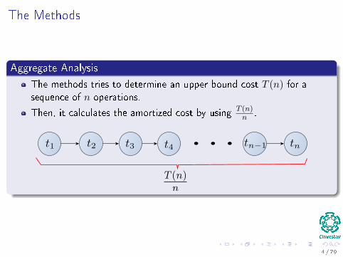
Aggregate Analysis
The methods tries to determine an upper bound cost T (n) for asequence of n operations.
Then, it calculates the amortized cost by using T (n)n .
4 / 79
The Methods
Aggregate Analysis
The methods tries to determine an upper bound cost T (n) for asequence of n operations.
Then, it calculates the amortized cost by using T (n)n .
4 / 79
The Methods
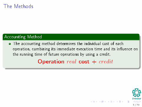
Accounting Method
The accounting method determines the individual cost of eachoperation, combining its immediate execution time and its in�uence onthe running time of future operations by using a credit.
Operation real cost + credit
5 / 79
The Methods
Accounting Method
The accounting method determines the individual cost of eachoperation, combining its immediate execution time and its in�uence onthe running time of future operations by using a credit.
Operation real cost + credit
5 / 79
The Methods
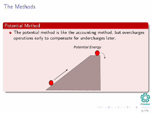
Potential Method
The potential method is like the accounting method, but overchargesoperations early to compensate for undercharges later.
Potential Energy
6 / 79
Aggregate Analysis
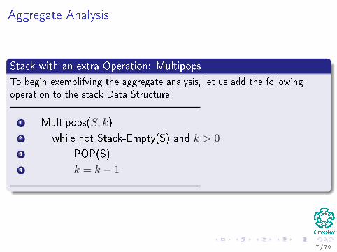
Stack with an extra Operation: Multipops
To begin exemplifying the aggregate analysis, let us add the followingoperation to the stack Data Structure.
1 Multipops(S, k)
2 while not Stack-Empty(S) and k > 0
3 POP(S)
4 k = k − 1
7 / 79
Aggregate Analysis
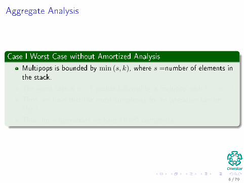
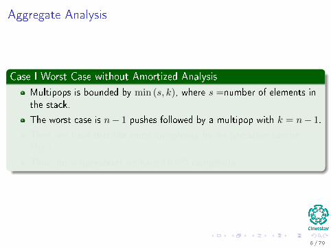
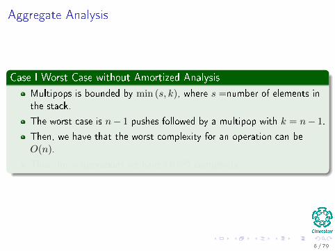
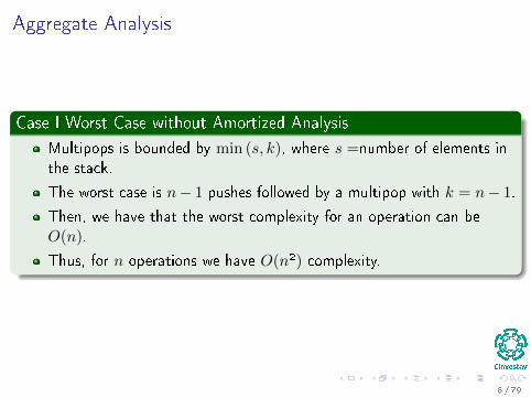
Case I Worst Case without Amortized Analysis
Multipops is bounded by min (s, k), where s =number of elements inthe stack.
The worst case is n− 1 pushes followed by a multipop with k = n− 1.
Then, we have that the worst complexity for an operation can beO(n).
Thus, for n operations we have O(n²) complexity.
8 / 79
Aggregate Analysis
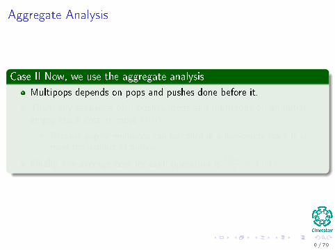
Case II Now, we use the aggregate analysis
Multipops depends on pops and pushes done before it.
Then, any sequence of n pushes, pops and multipops on an initialempty stack cost at most O(n)
I Because pop or multipops can be called in a non-empty stack is atmost the number of pushes.
Finally, the average cost for each operation is O(n)n = O(1).
9 / 79
Aggregate Analysis
Case II Now, we use the aggregate analysis
Multipops depends on pops and pushes done before it.
Then, any sequence of n pushes, pops and multipops on an initialempty stack cost at most O(n)
I Because pop or multipops can be called in a non-empty stack is atmost the number of pushes.
Finally, the average cost for each operation is O(n)n = O(1).
9 / 79
Example Binary Counter
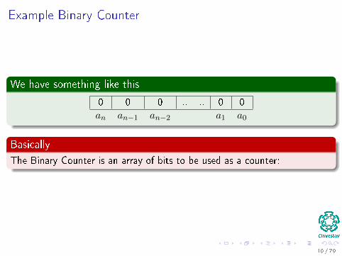
We have something like this
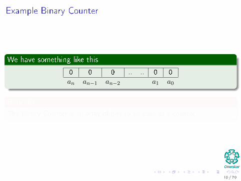
0 0 0 .. .. 0 0
an an−1 an−2 a1 a0
Basically
The Binary Counter is an array of bits to be used as a counter:
10 / 79
Example Binary Counter
We have something like this
0 0 0 .. .. 0 0
an an−1 an−2 a1 a0
Basically
The Binary Counter is an array of bits to be used as a counter:
10 / 79
Example Binary Counter
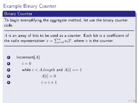
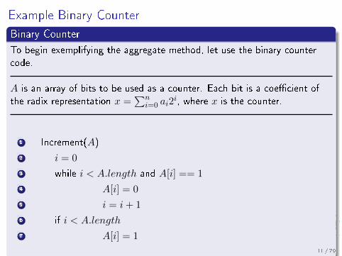
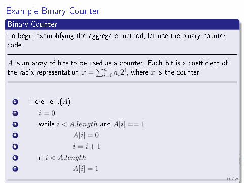
Binary Counter
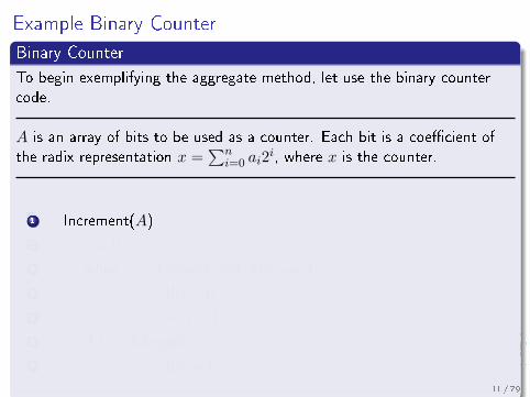
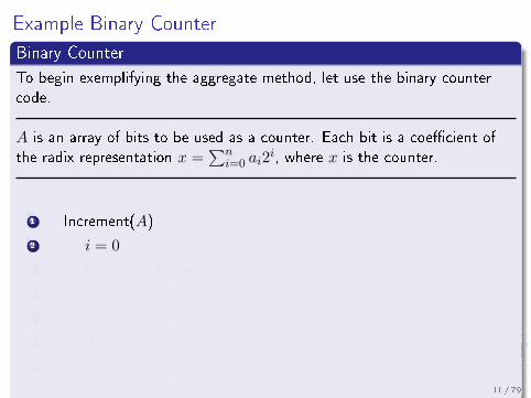
To begin exemplifying the aggregate method, let use the binary countercode.
A is an array of bits to be used as a counter. Each bit is a coe�cient ofthe radix representation x =
∑ni=0 ai2
i, where x is the counter.
1 Increment(A)
2 i = 0
3 while i < A.length and A[i] == 1
4 A[i] = 0
5 i = i+ 1
6 if i < A.length
7 A[i] = 1
11 / 79
Example Binary Counter
Binary Counter
To begin exemplifying the aggregate method, let use the binary countercode.
A is an array of bits to be used as a counter. Each bit is a coe�cient ofthe radix representation x =
∑ni=0 ai2
i, where x is the counter.
1 Increment(A)
2 i = 0
3 while i < A.length and A[i] == 1
4 A[i] = 0
5 i = i+ 1
6 if i < A.length
7 A[i] = 1
11 / 79
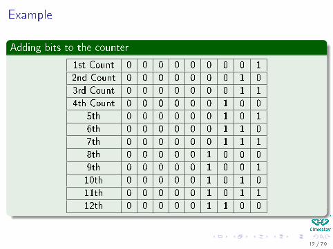
Example
Adding bits to the counter
1st Count 0 0 0 0 0 0 0 0 1
2nd Count 0 0 0 0 0 0 0 1 0
3rd Count 0 0 0 0 0 0 0 1 1
4th Count 0 0 0 0 0 0 1 0 0
5th 0 0 0 0 0 0 1 0 1
6th 0 0 0 0 0 0 1 1 0
7th 0 0 0 0 0 0 1 1 1
8th 0 0 0 0 0 1 0 0 0
9th 0 0 0 0 0 1 0 0 1
10th 0 0 0 0 0 1 0 1 0
11th 0 0 0 0 0 1 0 1 1
12th 0 0 0 0 0 1 1 0 0
12 / 79
Operations
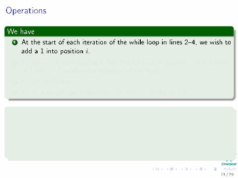
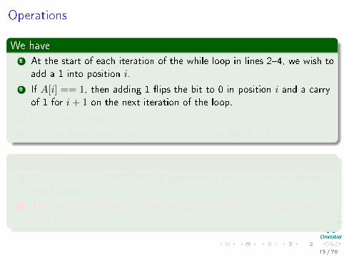
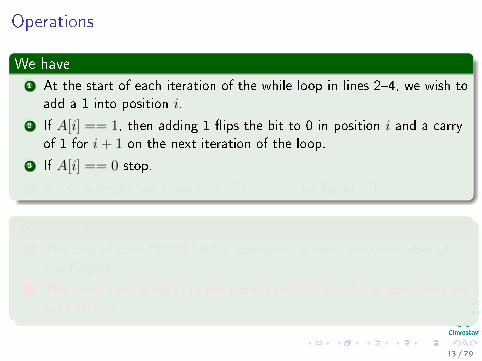
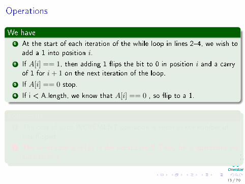
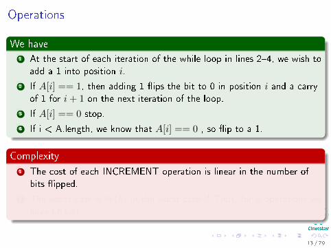
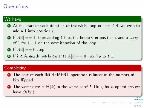
We have1 At the start of each iteration of the while loop in lines 2�4, we wish to
add a 1 into position i.
2 If A[i] == 1, then adding 1 �ips the bit to 0 in position i and a carryof 1 for i+ 1 on the next iteration of the loop.
3 If A[i] == 0 stop.
4 If i < A.length, we know that A[i] == 0 , so �ip to a 1.
Complexity
1 The cost of each INCREMENT operation is linear in the number ofbits �ipped.
2 The worst case is Θ (k) in the worst case!!! Thus, for n operations wehave O(kn).
13 / 79
Operations
We have1 At the start of each iteration of the while loop in lines 2�4, we wish to
add a 1 into position i.
2 If A[i] == 1, then adding 1 �ips the bit to 0 in position i and a carryof 1 for i+ 1 on the next iteration of the loop.
3 If A[i] == 0 stop.
4 If i < A.length, we know that A[i] == 0 , so �ip to a 1.
Complexity
1 The cost of each INCREMENT operation is linear in the number ofbits �ipped.
2 The worst case is Θ (k) in the worst case!!! Thus, for n operations wehave O(kn).
13 / 79
Better Analysis
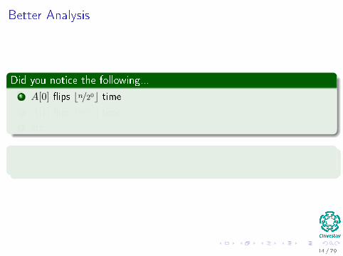
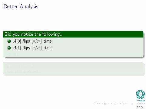
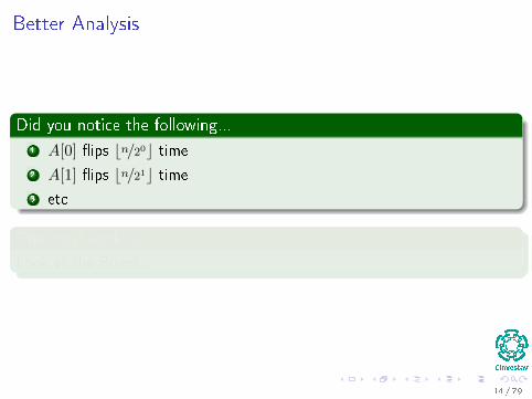
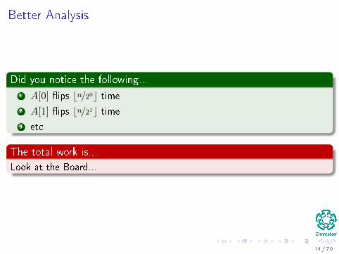
Did you notice the following...
1 A[0] �ips bn/20c time
2 A[1] �ips bn/21c time
3 etc
The total work is...
Look at the Board...
14 / 79
Better Analysis
Did you notice the following...
1 A[0] �ips bn/20c time
2 A[1] �ips bn/21c time
3 etc
The total work is...
Look at the Board...
14 / 79
Better Analysis
Did you notice the following...
1 A[0] �ips bn/20c time
2 A[1] �ips bn/21c time
3 etc
The total work is...
Look at the Board...
14 / 79
Better Analysis
Did you notice the following...
1 A[0] �ips bn/20c time
2 A[1] �ips bn/21c time
3 etc
The total work is...
Look at the Board...
14 / 79
Accounting Method
The use of credit
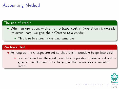
When an operation, with an amortized cost ci (operation i), exceedsits actual cost, we give the di�erence to a credit.
I This is to be stored in the data structure.
We have that
As long as the charges are set so that it is impossible to go into debt.
I one can show that there will never be an operation whose actual cost isgreater than the sum of its charge plus the previously accumulatedcredit.
15 / 79
Accounting Method
The use of credit
When an operation, with an amortized cost ci (operation i), exceedsits actual cost, we give the di�erence to a credit.
I This is to be stored in the data structure.
We have that
As long as the charges are set so that it is impossible to go into debt.
I one can show that there will never be an operation whose actual cost isgreater than the sum of its charge plus the previously accumulatedcredit.
15 / 79
More Formally
Something Notable
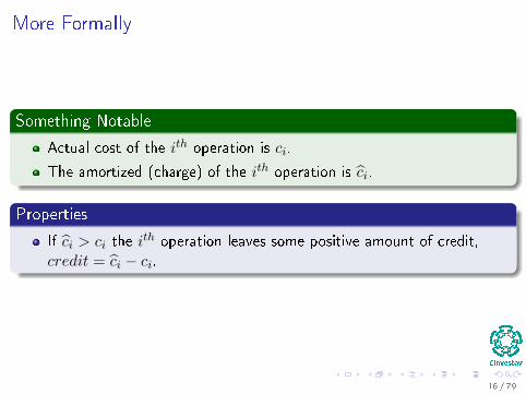
Actual cost of the ith operation is ci.
The amortized (charge) of the ith operation is ci.
Properties
If ci > ci the ith operation leaves some positive amount of credit,
credit = ci − ci.
16 / 79
More Formally
Something Notable
Actual cost of the ith operation is ci.
The amortized (charge) of the ith operation is ci.
Properties
If ci > ci the ith operation leaves some positive amount of credit,
credit = ci − ci.
16 / 79
More Formally
Something Notable
Actual cost of the ith operation is ci.
The amortized (charge) of the ith operation is ci.
Properties
If ci > ci the ith operation leaves some positive amount of credit,
credit = ci − ci.
16 / 79
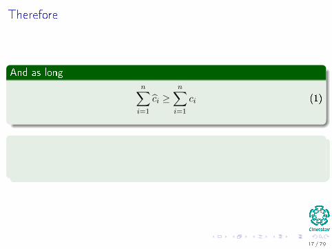
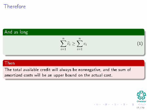
Therefore
And as longn∑
i=1
ci ≥n∑
i=1
ci (1)
Then
The total available credit will always be nonnegative, and the sum ofamortized costs will be an upper bound on the actual cost.
17 / 79
Therefore
And as longn∑
i=1
ci ≥n∑
i=1
ci (1)
Then
The total available credit will always be nonnegative, and the sum ofamortized costs will be an upper bound on the actual cost.
17 / 79
Outline
1 Introduction
2 What is this all about amortized analysis?
3 The Aggregate Method
4 The Accounting MethodBinary Counter
5 The Potential MethodStack Operations
6 Real Life ExamplesMove-To-Front (MTF)Dynamic Tables
Table Expansion
Aggegated Analysis
Potential Method
Table Expansions and Contractions
18 / 79
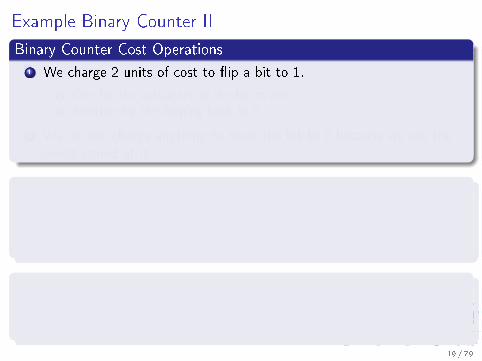
Example Binary Counter II
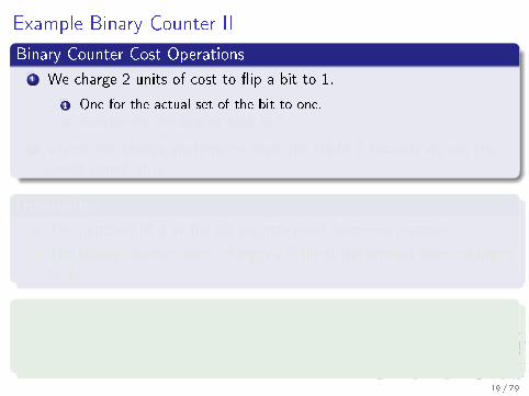
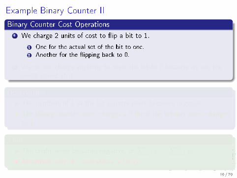
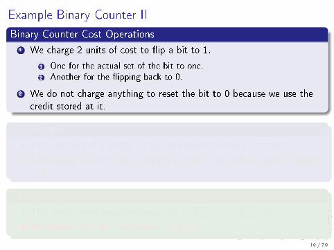
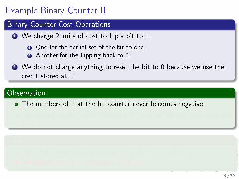
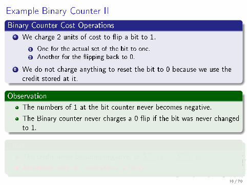
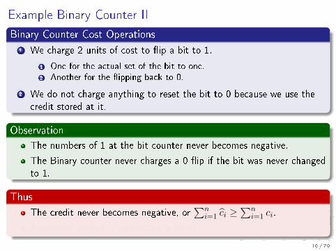
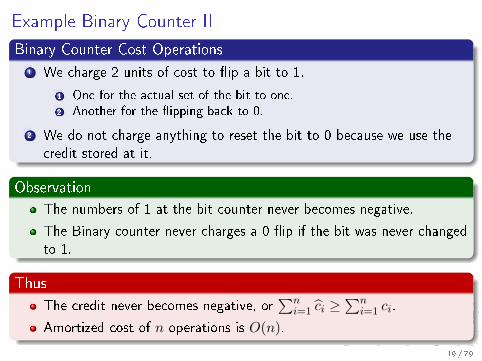
Binary Counter Cost Operations
1 We charge 2 units of cost to �ip a bit to 1.
1 One for the actual set of the bit to one.2 Another for the �ipping back to 0.
2 We do not charge anything to reset the bit to 0 because we use thecredit stored at it.
Observation
The numbers of 1 at the bit counter never becomes negative.
The Binary counter never charges a 0 �ip if the bit was never changedto 1.
Thus
The credit never becomes negative, or∑n
i=1 ci ≥∑n
i=1 ci.
Amortized cost of n operations is O(n).
19 / 79
Example Binary Counter II
Binary Counter Cost Operations
1 We charge 2 units of cost to �ip a bit to 1.
1 One for the actual set of the bit to one.2 Another for the �ipping back to 0.
2 We do not charge anything to reset the bit to 0 because we use thecredit stored at it.
Observation
The numbers of 1 at the bit counter never becomes negative.
The Binary counter never charges a 0 �ip if the bit was never changedto 1.
Thus
The credit never becomes negative, or∑n
i=1 ci ≥∑n
i=1 ci.
Amortized cost of n operations is O(n).
19 / 79
The Potential Method
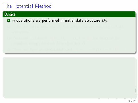
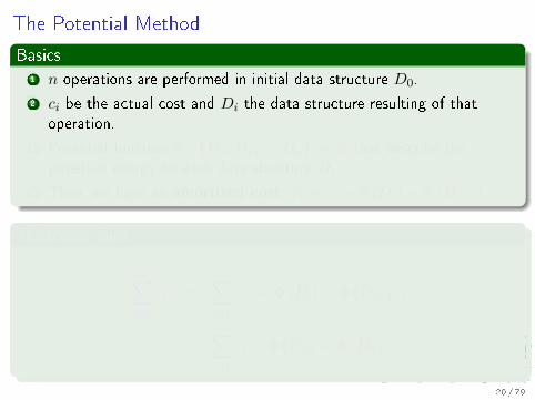
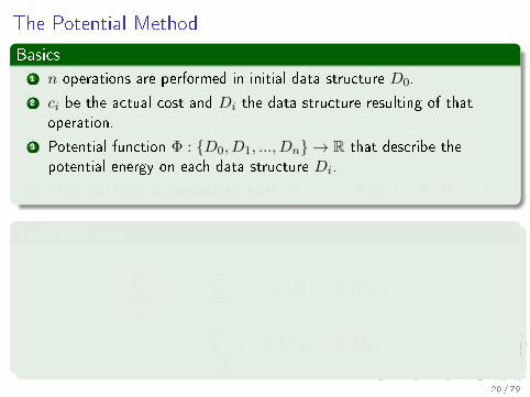
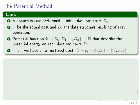
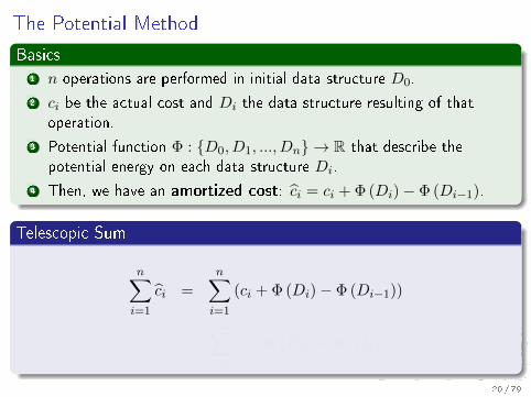
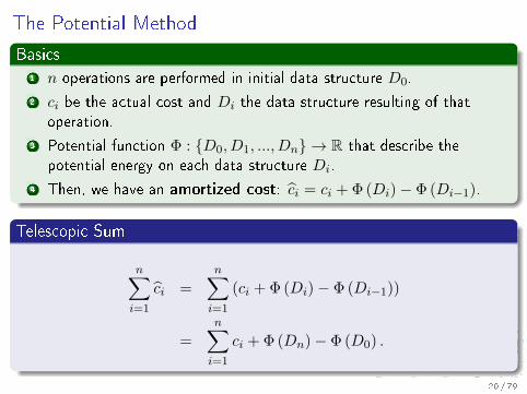
Basics1 n operations are performed in initial data structure D0.
2 ci be the actual cost and Di the data structure resulting of thatoperation.
3 Potential function Φ : {D0, D1, ..., Dn} → R that describe thepotential energy on each data structure Di.
4 Then, we have an amortized cost: ci = ci + Φ (Di)− Φ (Di−1).
Telescopic Sum
n∑i=1
ci =
n∑i=1
(ci + Φ (Di)− Φ (Di−1))
=
n∑i=1
ci + Φ (Dn)− Φ (D0) .
20 / 79
The Potential Method
Basics1 n operations are performed in initial data structure D0.
2 ci be the actual cost and Di the data structure resulting of thatoperation.
3 Potential function Φ : {D0, D1, ..., Dn} → R that describe thepotential energy on each data structure Di.
4 Then, we have an amortized cost: ci = ci + Φ (Di)− Φ (Di−1).
Telescopic Sum
n∑i=1
ci =
n∑i=1
(ci + Φ (Di)− Φ (Di−1))
=
n∑i=1
ci + Φ (Dn)− Φ (D0) .
20 / 79
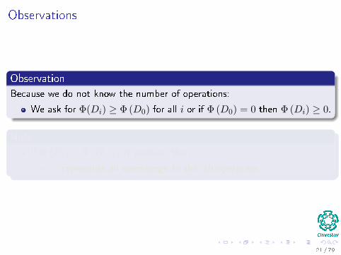
Observations
Observation
Because we do not know the number of operations:
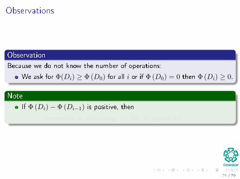
We ask for Φ(Di) ≥ Φ (D0) for all i or if Φ (D0) = 0 then Φ (Di) ≥ 0.
Note
If Φ (Di)− Φ (Di−1) is positive, then
I ci represents an overcharge to the ith operation.
21 / 79
Observations
Observation
Because we do not know the number of operations:
We ask for Φ(Di) ≥ Φ (D0) for all i or if Φ (D0) = 0 then Φ (Di) ≥ 0.
Note
If Φ (Di)− Φ (Di−1) is positive, then
I ci represents an overcharge to the ith operation.
21 / 79
Observations
Observation
Because we do not know the number of operations:
We ask for Φ(Di) ≥ Φ (D0) for all i or if Φ (D0) = 0 then Φ (Di) ≥ 0.
Note
If Φ (Di)− Φ (Di−1) is positive, then
I ci represents an overcharge to the ith operation.
21 / 79
Observations
Observation
Because we do not know the number of operations:
We ask for Φ(Di) ≥ Φ (D0) for all i or if Φ (D0) = 0 then Φ (Di) ≥ 0.
Note
If Φ (Di)− Φ (Di−1) is positive, then
I ci represents an overcharge to the ith operation.
21 / 79
Outline
1 Introduction
2 What is this all about amortized analysis?
3 The Aggregate Method
4 The Accounting MethodBinary Counter
5 The Potential MethodStack Operations
6 Real Life ExamplesMove-To-Front (MTF)Dynamic Tables
Table Expansion
Aggegated Analysis
Potential Method
Table Expansions and Contractions
22 / 79
Example Stack Operations I
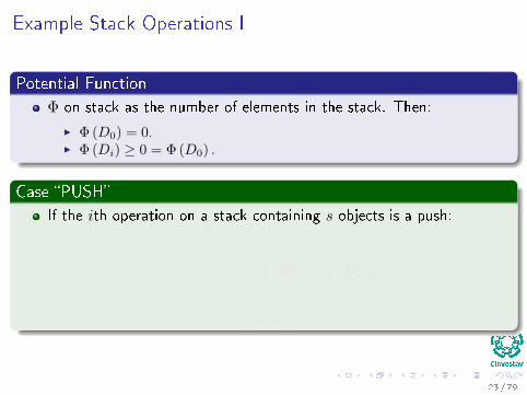
Potential Function
Φ on stack as the number of elements in the stack. Then:
I Φ (D0) = 0.I Φ (Di) ≥ 0 = Φ (D0) .
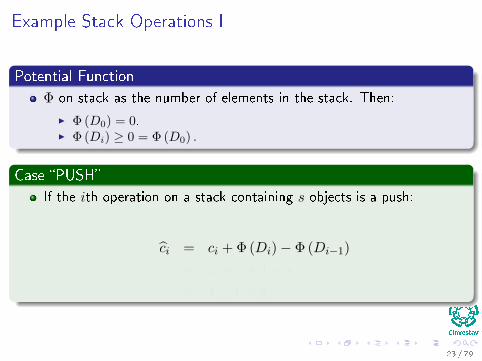
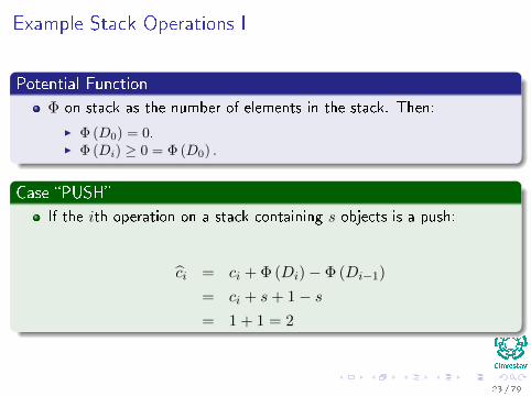
Case �PUSH�
If the ith operation on a stack containing s objects is a push:
ci = ci + Φ (Di)− Φ (Di−1)
= ci + s+ 1− s= 1 + 1 = 2
23 / 79
Example Stack Operations I
Potential Function
Φ on stack as the number of elements in the stack. Then:
I Φ (D0) = 0.I Φ (Di) ≥ 0 = Φ (D0) .
Case �PUSH�
If the ith operation on a stack containing s objects is a push:
ci = ci + Φ (Di)− Φ (Di−1)
= ci + s+ 1− s= 1 + 1 = 2
23 / 79
Example Stack Operations I
Potential Function
Φ on stack as the number of elements in the stack. Then:
I Φ (D0) = 0.I Φ (Di) ≥ 0 = Φ (D0) .
Case �PUSH�
If the ith operation on a stack containing s objects is a push:
ci = ci + Φ (Di)− Φ (Di−1)
= ci + s+ 1− s= 1 + 1 = 2
23 / 79
Example Stack Operations I
Potential Function
Φ on stack as the number of elements in the stack. Then:
I Φ (D0) = 0.I Φ (Di) ≥ 0 = Φ (D0) .
Case �PUSH�
If the ith operation on a stack containing s objects is a push:
ci = ci + Φ (Di)− Φ (Di−1)
= ci + s+ 1− s= 1 + 1 = 2
23 / 79

Example Stack Operations I
Potential Function
Φ on stack as the number of elements in the stack. Then:
I Φ (D0) = 0.I Φ (Di) ≥ 0 = Φ (D0) .
Case �PUSH�
If the ith operation on a stack containing s objects is a push:
ci = ci + Φ (Di)− Φ (Di−1)
= ci + s+ 1− s= 1 + 1 = 2
23 / 79
Example Stack Operations I
Potential Function
Φ on stack as the number of elements in the stack. Then:
I Φ (D0) = 0.I Φ (Di) ≥ 0 = Φ (D0) .
Case �PUSH�
If the ith operation on a stack containing s objects is a push:
ci = ci + Φ (Di)− Φ (Di−1)
= ci + s+ 1− s= 1 + 1 = 2
23 / 79
Example Stack Operations II
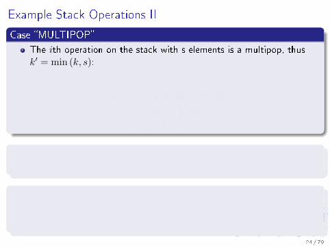
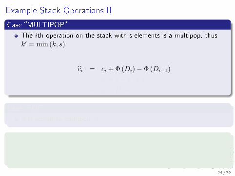
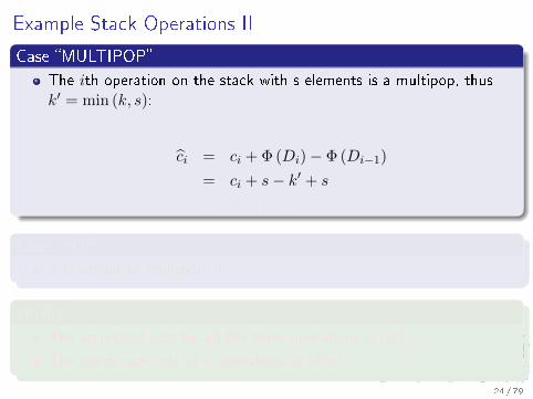
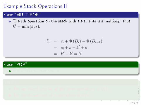
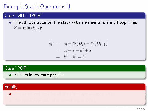
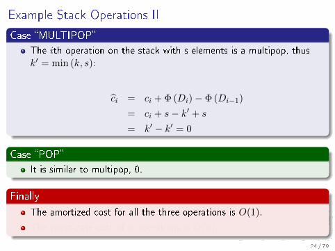
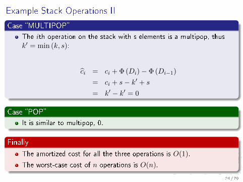
Case �MULTIPOP�
The ith operation on the stack with s elements is a multipop, thusk′ = min (k, s):
ci = ci + Φ (Di)− Φ (Di−1)
= ci + s− k′ + s
= k′ − k′ = 0
Case �POP�
It is similar to multipop, 0.
Finally
The amortized cost for all the three operations is O(1).
The worst-case cost of n operations is O(n).
24 / 79
Example Stack Operations II
Case �MULTIPOP�
The ith operation on the stack with s elements is a multipop, thusk′ = min (k, s):
ci = ci + Φ (Di)− Φ (Di−1)
= ci + s− k′ + s
= k′ − k′ = 0
Case �POP�
It is similar to multipop, 0.
Finally
The amortized cost for all the three operations is O(1).
The worst-case cost of n operations is O(n).
24 / 79
Outline
1 Introduction
2 What is this all about amortized analysis?
3 The Aggregate Method
4 The Accounting MethodBinary Counter
5 The Potential MethodStack Operations
6 Real Life ExamplesMove-To-Front (MTF)Dynamic Tables
Table Expansion
Aggegated Analysis
Potential Method
Table Expansions and Contractions
25 / 79
We have the following
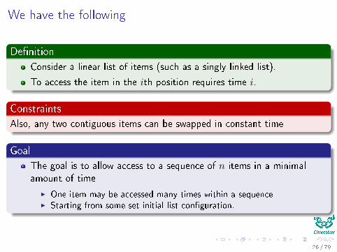
De�nition
Consider a linear list of items (such as a singly-linked list).
To access the item in the ith position requires time i.
Constraints
Also, any two contiguous items can be swapped in constant time
Goal
The goal is to allow access to a sequence of n items in a minimalamount of time
I One item may be accessed many times within a sequenceI Starting from some set initial list con�guration.
26 / 79
We have the following
De�nition
Consider a linear list of items (such as a singly-linked list).
To access the item in the ith position requires time i.
Constraints
Also, any two contiguous items can be swapped in constant time
Goal
The goal is to allow access to a sequence of n items in a minimalamount of time
I One item may be accessed many times within a sequenceI Starting from some set initial list con�guration.
26 / 79
Thus, we have two cases
First
If the sequence of accesses is known in advance, one can design an optimalalgorithm for swapping items to rearrange the list according to how oftenitems are accessed, and when.
Second
However, if the sequence is not known in advance, a heuristic method forswapping items may be desirable.
27 / 79
MTF Heuristic
Reality!!!
If item i is accessed at time t, it is likely to be accessed again soon aftertime t (i.e., there is locality of reference).
28 / 79
MTF Heuristic Example
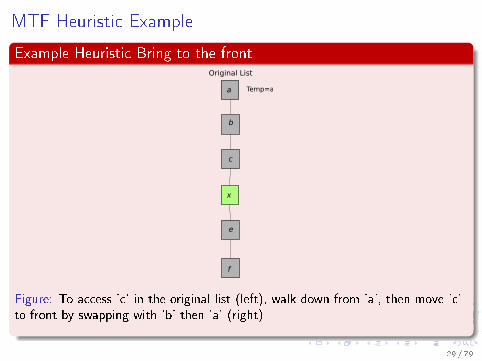
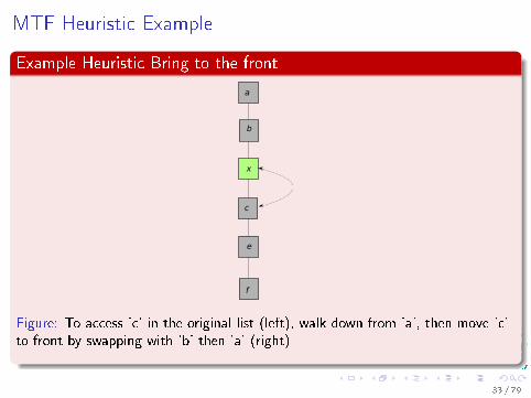
Example Heuristic Bring to the front
a
b
c
x
e
f
Original List
Temp=a
Figure: To access 'c' in the original list (left), walk down from 'a', then move 'c'to front by swapping with 'b' then 'a' (right)
29 / 79
MTF Heuristic Example
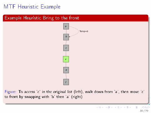
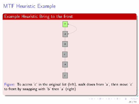
Example Heuristic Bring to the front
a
b
c
x
e
f
Temp=b
Figure: To access 'c' in the original list (left), walk down from 'a', then move 'c'to front by swapping with 'b' then 'a' (right)
30 / 79
MTF Heuristic Example
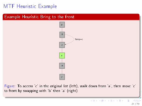
Example Heuristic Bring to the front
a
b
c
x
e
f
Temp=c
Figure: To access 'c' in the original list (left), walk down from 'a', then move 'c'to front by swapping with 'b' then 'a' (right)
31 / 79
MTF Heuristic Example
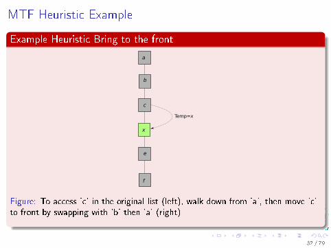
Example Heuristic Bring to the front
a
b
c
x
e
f
Temp=x
Figure: To access 'c' in the original list (left), walk down from 'a', then move 'c'to front by swapping with 'b' then 'a' (right)
32 / 79
MTF Heuristic Example
Example Heuristic Bring to the front
a
b
c
x
e
f
Figure: To access 'c' in the original list (left), walk down from 'a', then move 'c'to front by swapping with 'b' then 'a' (right)
33 / 79

MTF Heuristic Example
Example Heuristic Bring to the front
a
b
c
x
e
f
Figure: To access 'c' in the original list (left), walk down from 'a', then move 'c'to front by swapping with 'b' then 'a' (right)
34 / 79
MTF Heuristic Example
Example Heuristic Bring to the front
a
b
c
x
e
f
Figure: To access 'c' in the original list (left), walk down from 'a', then move 'c'to front by swapping with 'b' then 'a' (right)
35 / 79
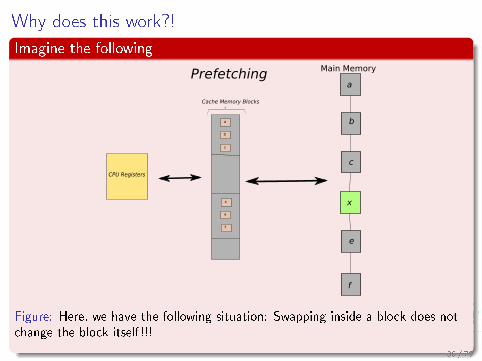
Why does this work?!
Imagine the following
a
b
c
x
e
f
Main Memory
a
b
c
x
e
f
CPU Registers
Cache Memory Blocks
Prefetching
Figure: Here, we have the following situation: Swapping inside a block does notchange the block itself!!!
36 / 79
Complexity of the Heuristic
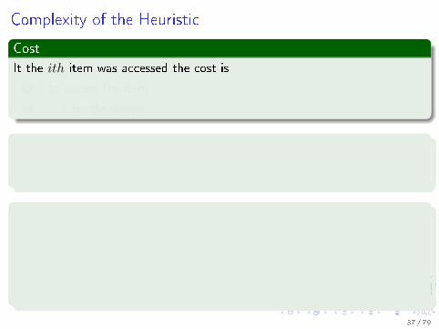
Cost
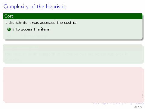
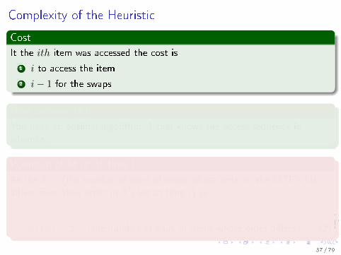
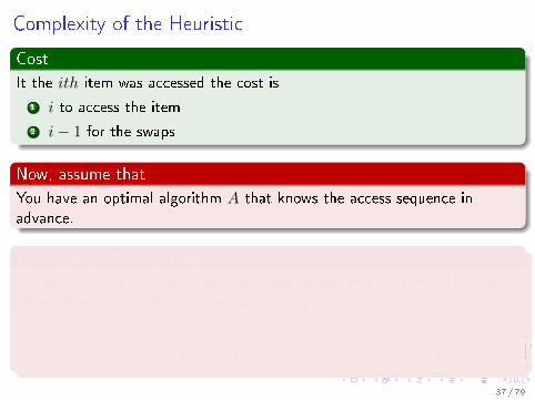
It the ith item was accessed the cost is
1 i to access the item
2 i− 1 for the swaps
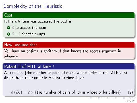
Now, assume that
You have an optimal algorithm A that knows the access sequence inadvance.
Potential of MTF at time t
As the 2 × {the number of pairs of items whose order in the MTF's listdi�ers from their order in A's list at time t} or
φ (Dt) = 2× {the number of pairs of items whose order di�ers} (2)
37 / 79
Complexity of the Heuristic
Cost
It the ith item was accessed the cost is
1 i to access the item
2 i− 1 for the swaps
Now, assume that
You have an optimal algorithm A that knows the access sequence inadvance.
Potential of MTF at time t
As the 2 × {the number of pairs of items whose order in the MTF's listdi�ers from their order in A's list at time t} or
φ (Dt) = 2× {the number of pairs of items whose order di�ers} (2)
37 / 79
Complexity of the Heuristic
For example
For example, if MTF's list is ordered (a, b, c, e, d) and A's list is ordered (a,b, c, d, e), then the potential for MTF will be equal to 2, because one pairof items (d and e) di�er in their ordering between A's list and MTF's list.
In addition
The potential at t = 0 is 0, as both algorithms begin with the samelist by de�nition.
Also, it is impossible for the potential to be negative.
38 / 79
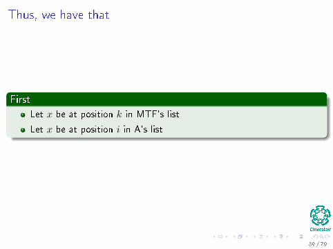
Thus, we have that
First
Let x be at position k in MTF's list
Let x be at position i in A's list
39 / 79
Thus, we have that
First
Let x be at position k in MTF's list
Let x be at position i in A's list
39 / 79
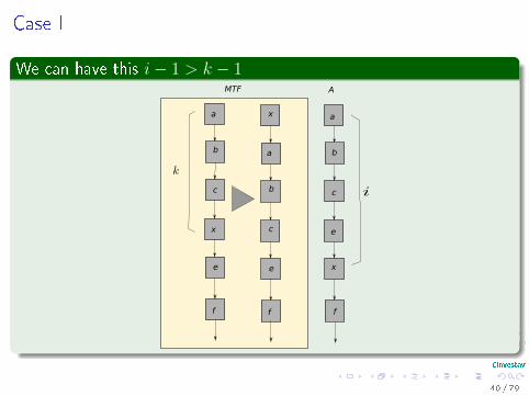
Case I
We can have this i− 1 > k − 1
a
b
c
x
xe
f
a
b
c
e
f
MTF A
a
b
c
x
e
f
40 / 79
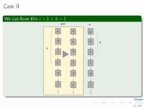
Case II
We can have this i− 1 < k − 1
a
b
c
x
x
e
f
a
b
c
e
f
MTF A
a
b
c
x
e
f
41 / 79
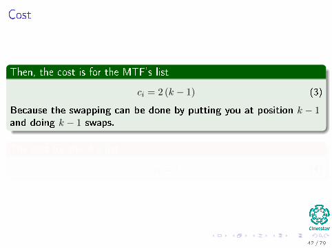
Cost
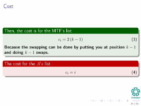
Then, the cost is for the MTF's list
ci = 2 (k − 1) (3)
Because the swapping can be done by putting you at position k − 1and doing k − 1 swaps.
The cost for the A′s list
ci = i (4)
42 / 79
Cost
Then, the cost is for the MTF's list
ci = 2 (k − 1) (3)
Because the swapping can be done by putting you at position k − 1and doing k − 1 swaps.
The cost for the A′s list
ci = i (4)
42 / 79
Then
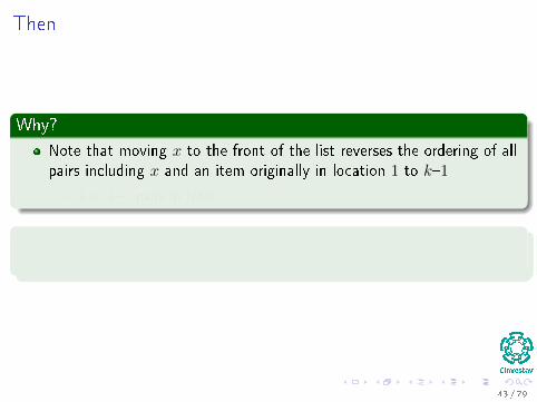
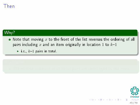
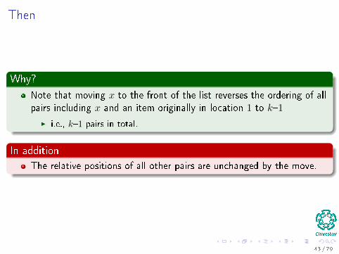
Why?
Note that moving x to the front of the list reverses the ordering of allpairs including x and an item originally in location 1 to k�1
I i.e., k�1 pairs in total.
In addition
The relative positions of all other pairs are unchanged by the move.
43 / 79
Then
Why?
Note that moving x to the front of the list reverses the ordering of allpairs including x and an item originally in location 1 to k�1
I i.e., k�1 pairs in total.
In addition
The relative positions of all other pairs are unchanged by the move.
43 / 79
Then
Why?
Note that moving x to the front of the list reverses the ordering of allpairs including x and an item originally in location 1 to k�1
I i.e., k�1 pairs in total.
In addition
The relative positions of all other pairs are unchanged by the move.
43 / 79
What is φ (Dt)− φ (Dt−1)?
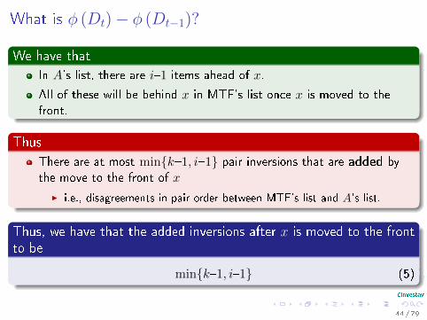
We have that
In A's list, there are i�1 items ahead of x.
All of these will be behind x in MTF's list once x is moved to thefront.
Thus
There are at most min{k�1, i�1} pair inversions that are added bythe move to the front of x
I i.e., disagreements in pair order between MTF's list and A's list.
Thus, we have that the added inversions after x is moved to the frontto be
min{k�1, i�1} (5)
44 / 79
What is φ (Dt)− φ (Dt−1)?
We have that
In A's list, there are i�1 items ahead of x.
All of these will be behind x in MTF's list once x is moved to thefront.
Thus
There are at most min{k�1, i�1} pair inversions that are added bythe move to the front of x
I i.e., disagreements in pair order between MTF's list and A's list.
Thus, we have that the added inversions after x is moved to the frontto be
min{k�1, i�1} (5)
44 / 79
Now, What about ?
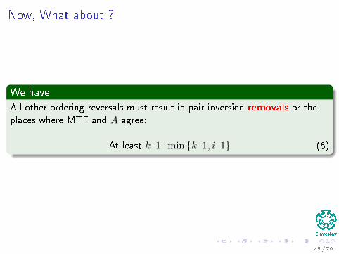
We have
All other ordering reversals must result in pair inversion removals or theplaces where MTF and A agree:
At least k�1�min {k�1, i�1} (6)
45 / 79
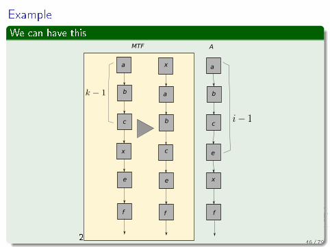
Example
We can have this
2
a
b
c
x
xe
f
a
b
c
e
f
MTF A
a
b
c
x
e
f
46 / 79
Then
We have that
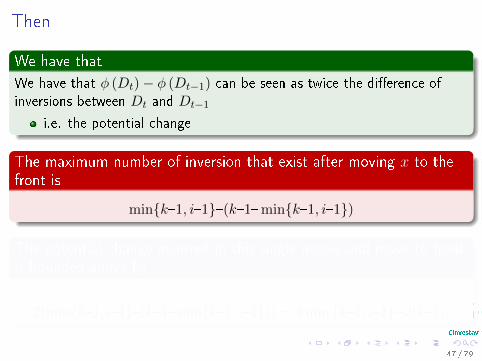
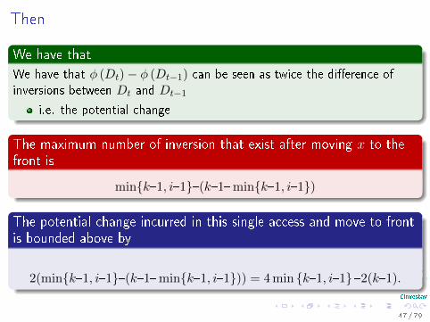
We have that φ (Dt)− φ (Dt−1) can be seen as twice the di�erence ofinversions between Dt and Dt−1
i.e. the potential change
The maximum number of inversion that exist after moving x to thefront is
min{k�1, i�1}�(k�1�min{k�1, i�1})
The potential change incurred in this single access and move to frontis bounded above by
2(min{k�1, i�1}�(k�1�min{k�1, i�1})) = 4 min {k�1, i�1} �2(k�1).
47 / 79
Then
We have that
We have that φ (Dt)− φ (Dt−1) can be seen as twice the di�erence ofinversions between Dt and Dt−1
i.e. the potential change
The maximum number of inversion that exist after moving x to thefront is
min{k�1, i�1}�(k�1�min{k�1, i�1})
The potential change incurred in this single access and move to frontis bounded above by
2(min{k�1, i�1}�(k�1�min{k�1, i�1})) = 4 min {k�1, i�1} �2(k�1).
47 / 79
Using the Upper Bound of the Potential Change
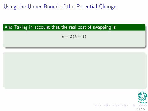
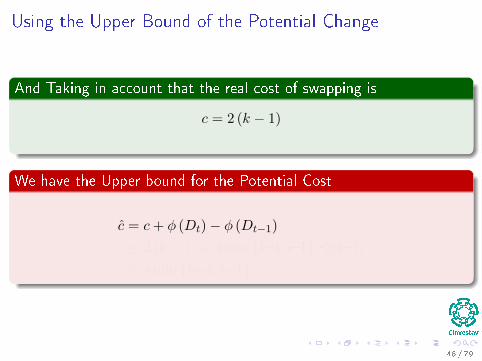
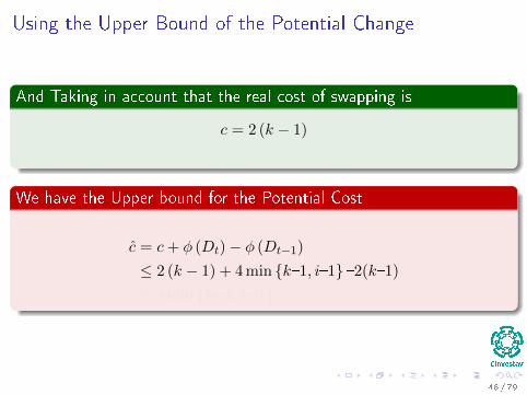
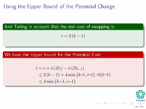
And Taking in account that the real cost of swapping is
c = 2 (k − 1)
We have the Upper bound for the Potential Cost
c = c+ φ (Dt)− φ (Dt−1)
≤ 2 (k − 1) + 4 min {k�1, i�1} �2(k�1)
≤ 4 min {k=1, i=1}
48 / 79
Using the Upper Bound of the Potential Change
And Taking in account that the real cost of swapping is
c = 2 (k − 1)
We have the Upper bound for the Potential Cost
c = c+ φ (Dt)− φ (Dt−1)
≤ 2 (k − 1) + 4 min {k�1, i�1} �2(k�1)
≤ 4 min {k=1, i=1}
48 / 79
Using the Upper Bound of the Potential Change
And Taking in account that the real cost of swapping is
c = 2 (k − 1)
We have the Upper bound for the Potential Cost
c = c+ φ (Dt)− φ (Dt−1)
≤ 2 (k − 1) + 4 min {k�1, i�1} �2(k�1)
≤ 4 min {k=1, i=1}
48 / 79
Using the Upper Bound of the Potential Change
And Taking in account that the real cost of swapping is
c = 2 (k − 1)
We have the Upper bound for the Potential Cost
c = c+ φ (Dt)− φ (Dt−1)
≤ 2 (k − 1) + 4 min {k�1, i�1} �2(k�1)
≤ 4 min {k=1, i=1}
48 / 79
Potential Change
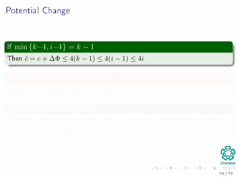
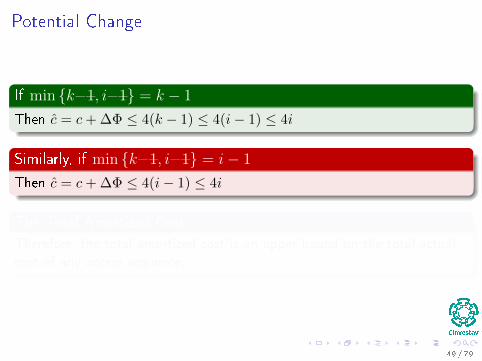
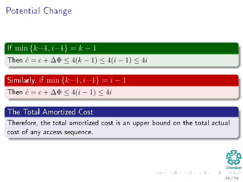
If min {k=1, i=1} = k − 1
Then c = c+ ∆Φ ≤ 4(k − 1) ≤ 4(i− 1) ≤ 4i
Similarly, if min {k=1, i=1} = i− 1
Then c = c+ ∆Φ ≤ 4(i− 1) ≤ 4i
The Total Amortized Cost
Therefore, the total amortized cost is an upper bound on the total actualcost of any access sequence.
49 / 79
Potential Change
If min {k=1, i=1} = k − 1
Then c = c+ ∆Φ ≤ 4(k − 1) ≤ 4(i− 1) ≤ 4i
Similarly, if min {k=1, i=1} = i− 1
Then c = c+ ∆Φ ≤ 4(i− 1) ≤ 4i
The Total Amortized Cost
Therefore, the total amortized cost is an upper bound on the total actualcost of any access sequence.
49 / 79
Potential Change
If min {k=1, i=1} = k − 1
Then c = c+ ∆Φ ≤ 4(k − 1) ≤ 4(i− 1) ≤ 4i
Similarly, if min {k=1, i=1} = i− 1
Then c = c+ ∆Φ ≤ 4(i− 1) ≤ 4i
The Total Amortized Cost
Therefore, the total amortized cost is an upper bound on the total actualcost of any access sequence.
49 / 79
Finally
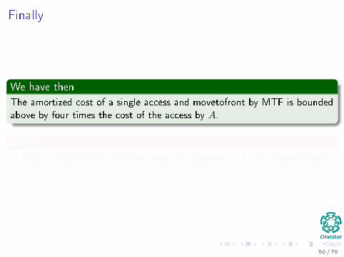
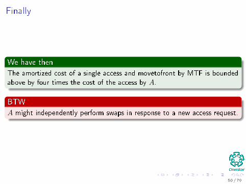
We have then
The amortized cost of a single access and movetofront by MTF is boundedabove by four times the cost of the access by A.
BTW
A might independently perform swaps in response to a new access request.
50 / 79
Finally
We have then
The amortized cost of a single access and movetofront by MTF is boundedabove by four times the cost of the access by A.
BTW
A might independently perform swaps in response to a new access request.
50 / 79
For example
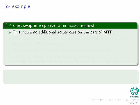
If A does swap in response to an access request.
This incurs no additional actual cost on the part of MTF.
But it will increase or decrease the new potential by 2 and the costaccess of A will increase by 1.
The bound on MTF's amortized cost still holds because
I The amortized cost is increased by at most 2I but the bound is increased by 4 (Remember the multiplication by 2)
Not only that
This is true no matter how many swap operations A performs.
51 / 79
For example
If A does swap in response to an access request.
This incurs no additional actual cost on the part of MTF.
But it will increase or decrease the new potential by 2 and the costaccess of A will increase by 1.
The bound on MTF's amortized cost still holds because
I The amortized cost is increased by at most 2I but the bound is increased by 4 (Remember the multiplication by 2)
Not only that
This is true no matter how many swap operations A performs.
51 / 79
Final words
Using a MTF is more e�cient
Because in order to device A, it will require complex statisticestimators
Against a simple MTF algorithm...
52 / 79
Final words
Using a MTF is more e�cient
Because in order to device A, it will require complex statisticestimators
Against a simple MTF algorithm...
52 / 79

Outline
1 Introduction
2 What is this all about amortized analysis?
3 The Aggregate Method
4 The Accounting MethodBinary Counter
5 The Potential MethodStack Operations
6 Real Life ExamplesMove-To-Front (MTF)Dynamic Tables
Table Expansion
Aggegated Analysis
Potential Method
Table Expansions and Contractions
53 / 79
Dynamic Tables
De�nition
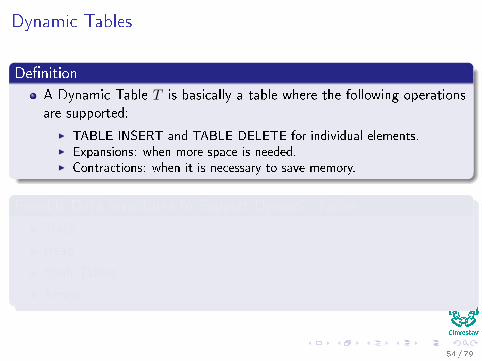
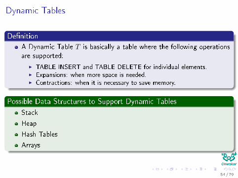
A Dynamic Table T is basically a table where the following operationsare supported:
I TABLE-INSERT and TABLE-DELETE for individual elements.I Expansions: when more space is needed.I Contractions: when it is necessary to save memory.
Possible Data Structures to Support Dynamic Tables
Stack
Heap
Hash Tables
Arrays
54 / 79
Dynamic Tables
De�nition
A Dynamic Table T is basically a table where the following operationsare supported:
I TABLE-INSERT and TABLE-DELETE for individual elements.I Expansions: when more space is needed.I Contractions: when it is necessary to save memory.
Possible Data Structures to Support Dynamic Tables
Stack
Heap
Hash Tables
Arrays
54 / 79
Dynamic Tables
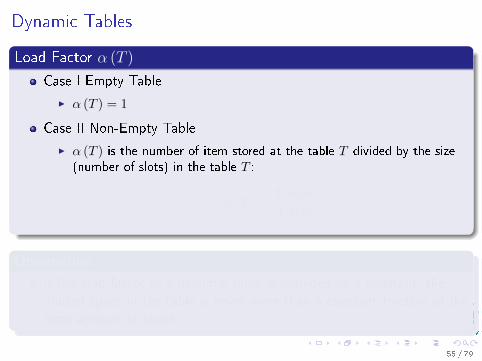
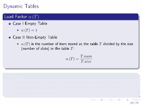
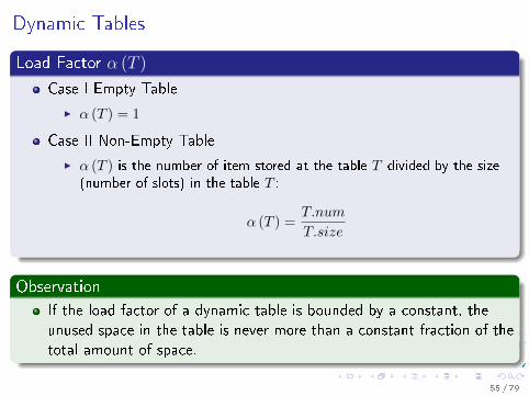
Load Factor α (T )
Case I Empty Table
I α (T ) = 1
Case II Non-Empty Table
I α (T ) is the number of item stored at the table T divided by the size(number of slots) in the table T :
α (T ) =T.num
T.size
Observation
If the load factor of a dynamic table is bounded by a constant, theunused space in the table is never more than a constant fraction of thetotal amount of space.
55 / 79
Dynamic Tables
Load Factor α (T )
Case I Empty Table
I α (T ) = 1
Case II Non-Empty Table
I α (T ) is the number of item stored at the table T divided by the size(number of slots) in the table T :
α (T ) =T.num
T.size
Observation
If the load factor of a dynamic table is bounded by a constant, theunused space in the table is never more than a constant fraction of thetotal amount of space.
55 / 79
Table Expansion
Heuristic
Allocate a new table with twice the size when T.num = T.size.
We have only insertions:
I The Load Factor is always ≥ 12 .
I Wasted space is never more than half the space.
CodeTable-Insert(T, x)
1 if T.size == 0
2 allocate T.table with 1 slot
3 T.size = 1
4 if T.size == T.num
5 allocate new − table with 2 · T.size slots
6 insert items in T.table into new − table
7 free T.table, T.table = new − table and T.size = 2 · T.size8 insert x into T.table
9 T.num = T.num+ 1 56 / 79
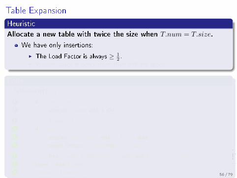
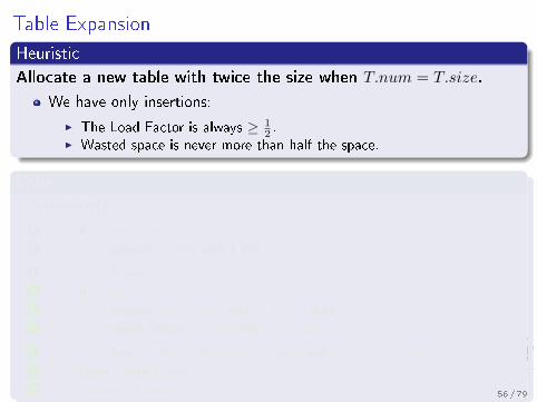
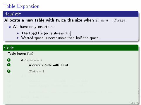
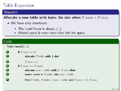
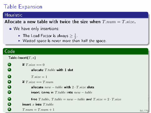
Aggregated Analysis
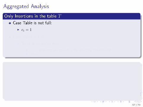
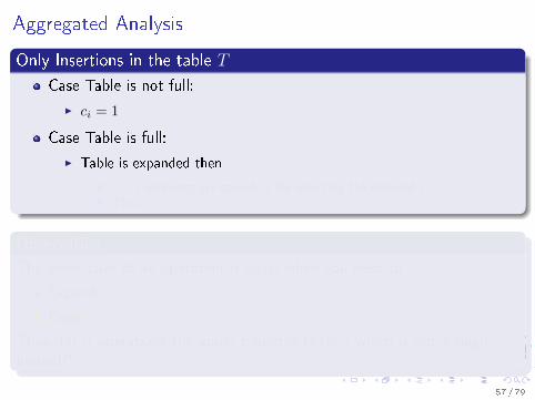
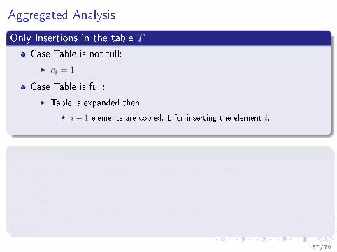
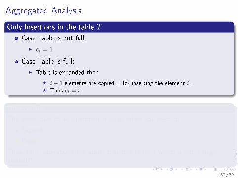
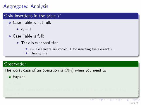
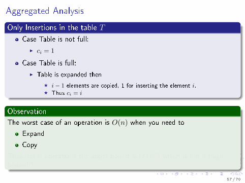
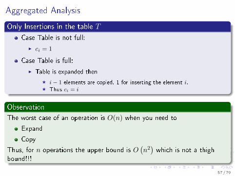
Only Insertions in the table T
Case Table is not full:
I ci = 1
Case Table is full:
I Table is expanded then
F i− 1 elements are copied, 1 for inserting the element i.F Thus ci = i
Observation
The worst case of an operation is O(n) when you need to
Expand
Copy
Thus, for n operations the upper bound is O(n2)which is not a thigh
bound!!!
57 / 79
Aggregated Analysis
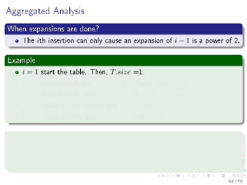
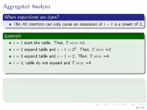
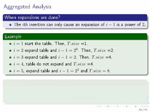
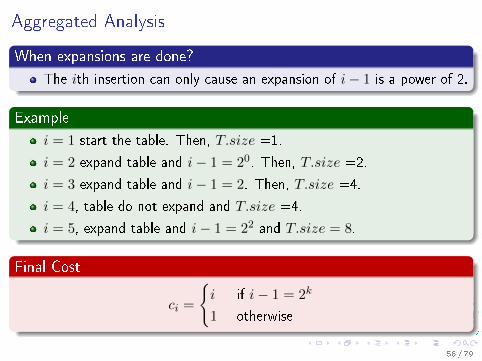
When expansions are done?
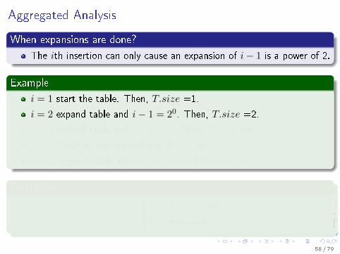
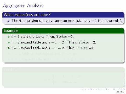
The ith insertion can only cause an expansion of i− 1 is a power of 2.
Example
i = 1 start the table. Then, T.size =1.
i = 2 expand table and i− 1 = 20. Then, T.size =2.
i = 3 expand table and i− 1 = 2. Then, T.size =4.
i = 4, table do not expand and T.size =4.
i = 5, expand table and i− 1 = 22 and T.size = 8.
Final Cost
ci =
{i if i− 1 = 2k
1 otherwise
58 / 79
Aggregated Analysis
When expansions are done?
The ith insertion can only cause an expansion of i− 1 is a power of 2.
Example
i = 1 start the table. Then, T.size =1.
i = 2 expand table and i− 1 = 20. Then, T.size =2.
i = 3 expand table and i− 1 = 2. Then, T.size =4.
i = 4, table do not expand and T.size =4.
i = 5, expand table and i− 1 = 22 and T.size = 8.
Final Cost
ci =
{i if i− 1 = 2k
1 otherwise
58 / 79
Aggregated Analysis
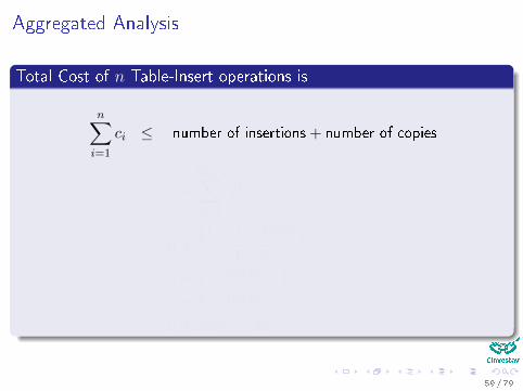
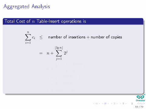
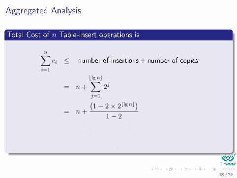
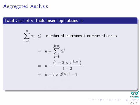
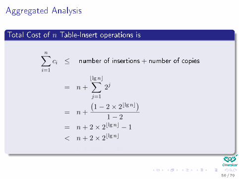
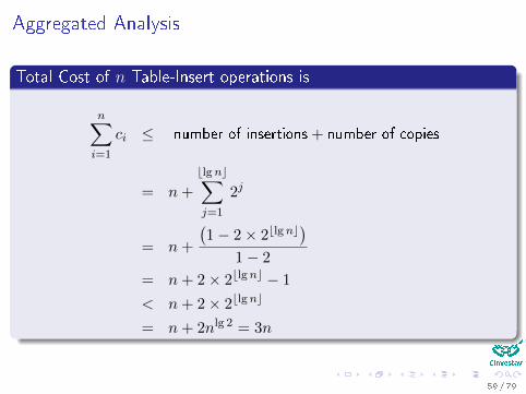
Total Cost of n Table-Insert operations is
n∑i=1
ci ≤ number of insertions + number of copies
= n+
blgnc∑j=1
2j
= n+
(1− 2× 2blgnc
)1− 2
= n+ 2× 2blgnc − 1
< n+ 2× 2blgnc
= n+ 2nlg 2 = 3n
59 / 79
Aggregated Analysis
Total Cost of n Table-Insert operations is
n∑i=1
ci ≤ number of insertions + number of copies
= n+
blgnc∑j=1
2j
= n+
(1− 2× 2blgnc
)1− 2
= n+ 2× 2blgnc − 1
< n+ 2× 2blgnc
= n+ 2nlg 2 = 3n
59 / 79
Aggregated Analysis
Total Cost of n Table-Insert operations is
n∑i=1
ci ≤ number of insertions + number of copies
= n+
blgnc∑j=1
2j
= n+
(1− 2× 2blgnc
)1− 2
= n+ 2× 2blgnc − 1
< n+ 2× 2blgnc
= n+ 2nlg 2 = 3n
59 / 79
Aggregated Analysis
Total Cost of n Table-Insert operations is
n∑i=1
ci ≤ number of insertions + number of copies
= n+
blgnc∑j=1
2j
= n+
(1− 2× 2blgnc
)1− 2
= n+ 2× 2blgnc − 1
< n+ 2× 2blgnc
= n+ 2nlg 2 = 3n
59 / 79
Aggregated Analysis
Total Cost of n Table-Insert operations is
n∑i=1
ci ≤ number of insertions + number of copies
= n+
blgnc∑j=1
2j
= n+
(1− 2× 2blgnc
)1− 2
= n+ 2× 2blgnc − 1
< n+ 2× 2blgnc
= n+ 2nlg 2 = 3n
59 / 79
Aggregated Analysis
Total Cost of n Table-Insert operations is
n∑i=1
ci ≤ number of insertions + number of copies
= n+
blgnc∑j=1
2j
= n+
(1− 2× 2blgnc
)1− 2
= n+ 2× 2blgnc − 1
< n+ 2× 2blgnc
= n+ 2nlg 2 = 3n
59 / 79
Potential Method
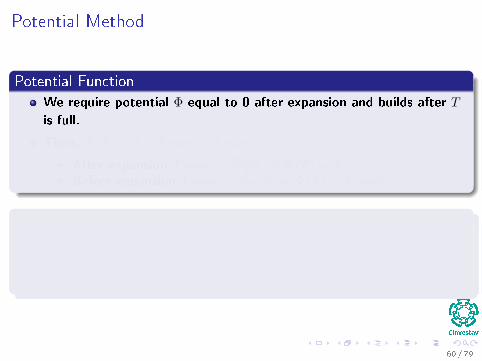
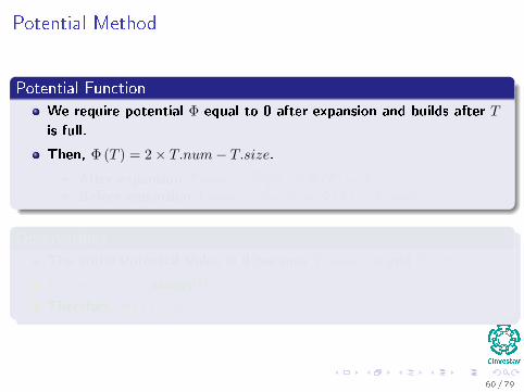
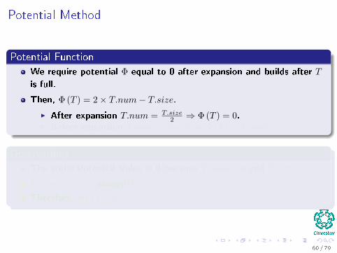
Potential Function
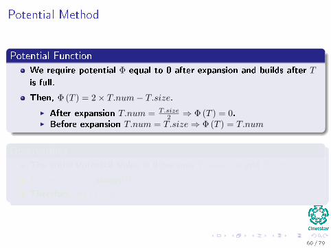
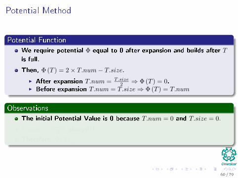
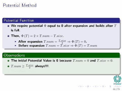
We require potential Φ equal to 0 after expansion and builds after T
is full.
Then, Φ (T ) = 2× T.num− T.size.I After expansion T.num = T.size
2 ⇒ Φ (T ) = 0.I Before expansion T.num = T.size⇒ Φ (T ) = T.num
Observations
The initial Potential Value is 0 because T.num = 0 and T.size = 0.
T.num ≥ T.size2 always!!!.
Therefore, Φ (T ) ≥ 0
60 / 79
Potential Method
Potential Function
We require potential Φ equal to 0 after expansion and builds after T
is full.
Then, Φ (T ) = 2× T.num− T.size.I After expansion T.num = T.size
2 ⇒ Φ (T ) = 0.I Before expansion T.num = T.size⇒ Φ (T ) = T.num
Observations
The initial Potential Value is 0 because T.num = 0 and T.size = 0.
T.num ≥ T.size2 always!!!.
Therefore, Φ (T ) ≥ 0
60 / 79
Potential Method
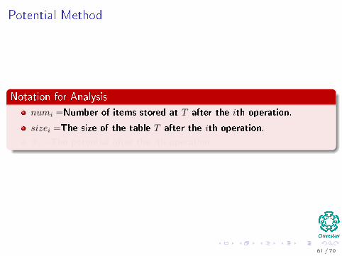
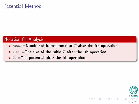
Notation for Analysis
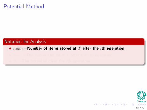
numi =Number of items stored at T after the ith operation.
sizei =The size of the table T after the ith operation.
Φi =The potential after the ith operation.
61 / 79
Potential Method
Notation for Analysis
numi =Number of items stored at T after the ith operation.
sizei =The size of the table T after the ith operation.
Φi =The potential after the ith operation.
61 / 79
Potential Method
Notation for Analysis
numi =Number of items stored at T after the ith operation.
sizei =The size of the table T after the ith operation.
Φi =The potential after the ith operation.
61 / 79
Potential Method
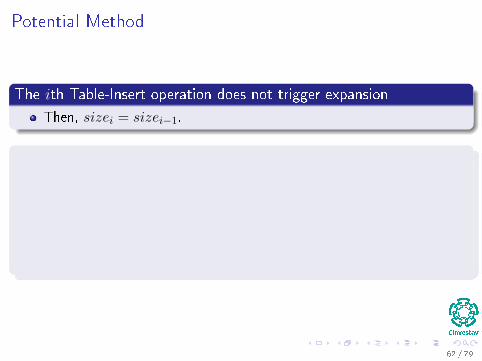
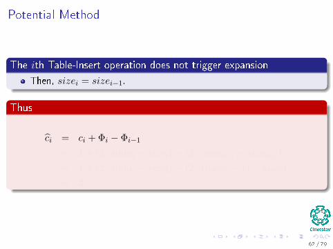
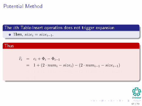
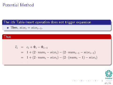
The ith Table-Insert operation does not trigger expansion
Then, sizei = sizei−1.
Thus
ci = ci + Φi − Φi−1
= 1 + (2 · numi − sizei)− (2 · numi−1 − sizei−1)= 1 + (2 · numi − sizei)− (2 · (numi − 1)− sizei)= 3
62 / 79
Potential Method
The ith Table-Insert operation does not trigger expansion
Then, sizei = sizei−1.
Thus
ci = ci + Φi − Φi−1
= 1 + (2 · numi − sizei)− (2 · numi−1 − sizei−1)= 1 + (2 · numi − sizei)− (2 · (numi − 1)− sizei)= 3
62 / 79
Potential Method
The ith Table-Insert operation does not trigger expansion
Then, sizei = sizei−1.
Thus
ci = ci + Φi − Φi−1
= 1 + (2 · numi − sizei)− (2 · numi−1 − sizei−1)= 1 + (2 · numi − sizei)− (2 · (numi − 1)− sizei)= 3
62 / 79
Potential Method
The ith Table-Insert operation does not trigger expansion
Then, sizei = sizei−1.
Thus
ci = ci + Φi − Φi−1
= 1 + (2 · numi − sizei)− (2 · numi−1 − sizei−1)= 1 + (2 · numi − sizei)− (2 · (numi − 1)− sizei)= 3
62 / 79

Potential Method
The ith Table-Insert operation does not trigger expansion
Then, sizei = sizei−1.
Thus
ci = ci + Φi − Φi−1
= 1 + (2 · numi − sizei)− (2 · numi−1 − sizei−1)= 1 + (2 · numi − sizei)− (2 · (numi − 1)− sizei)= 3
62 / 79
Potential Method
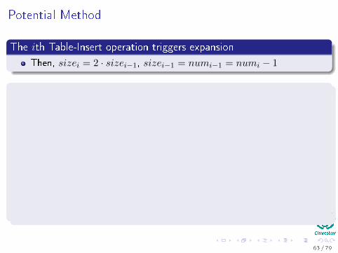
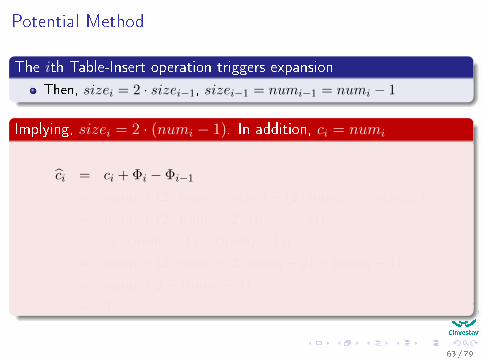
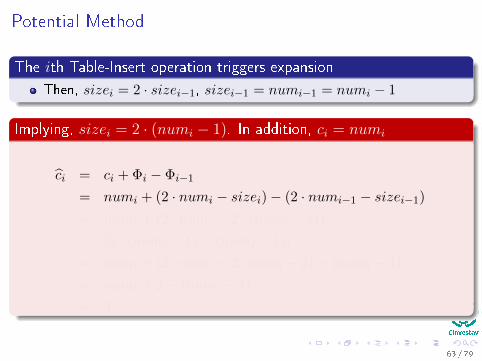
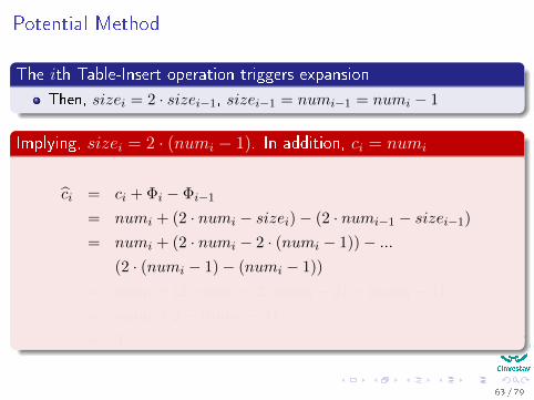
The ith Table-Insert operation triggers expansion
Then, sizei = 2 · sizei−1, sizei−1 = numi−1 = numi − 1
Implying, sizei = 2 · (numi − 1). In addition, ci = numi
ci = ci + Φi − Φi−1
= numi + (2 · numi − sizei)− (2 · numi−1 − sizei−1)= numi + (2 · numi − 2 · (numi − 1))− ...
(2 · (numi − 1)− (numi − 1))
= numi + (2 · numi − 2 · numi − 2)− (numi − 1)
= numi + 2− (numi − 1)
= 3
63 / 79
Potential Method
The ith Table-Insert operation triggers expansion
Then, sizei = 2 · sizei−1, sizei−1 = numi−1 = numi − 1
Implying, sizei = 2 · (numi − 1). In addition, ci = numi
ci = ci + Φi − Φi−1
= numi + (2 · numi − sizei)− (2 · numi−1 − sizei−1)= numi + (2 · numi − 2 · (numi − 1))− ...
(2 · (numi − 1)− (numi − 1))
= numi + (2 · numi − 2 · numi − 2)− (numi − 1)
= numi + 2− (numi − 1)
= 3
63 / 79
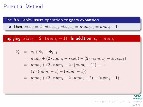
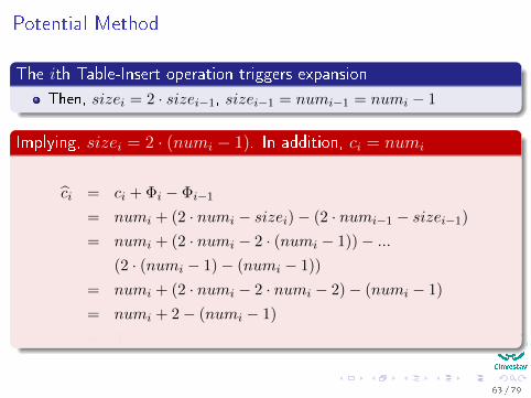
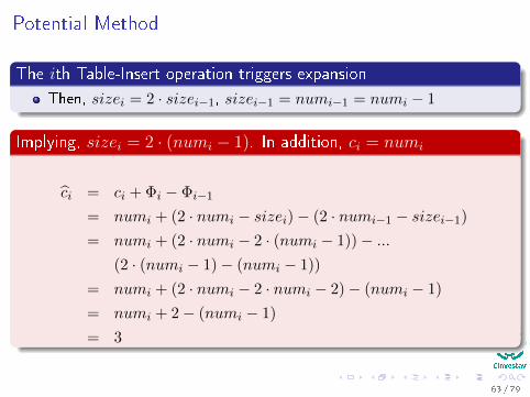
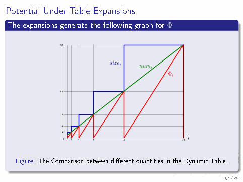
Potential Under Table Expansions
The expansions generate the following graph for Φ
2
2 4 8 16
4
8
16
32
1 320
Figure: The Comparison between di�erent quantities in the Dynamic Table.
64 / 79
Table Expansions and Contractions
Properties to be maintained
The load factor of the dynamic table is bounded below by a positiveconstant.
The amortized cost of a table operation is bounded above by aconstant.
Possible Heuristic, but not the correct one
You double the table when inserting an item into a full table.
You halve the table size, when deleting an item causes the table tobecome less than half full.
65 / 79
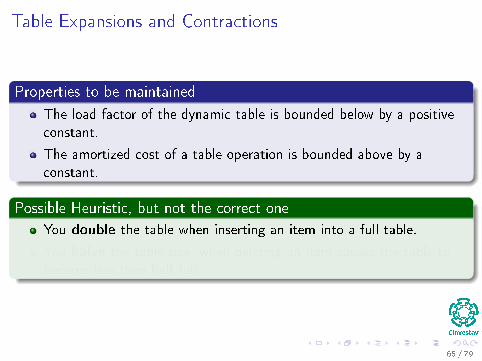
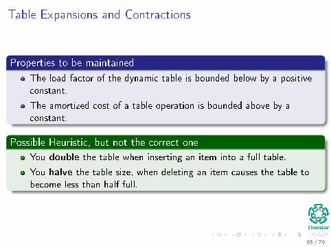
Table Expansions and Contractions
Problem!!!
You could have n = 2t insertions and deletions in a sequence in thefollowing sequence:
First n2 operations are insertions, thus T.num = T.size = n
2 .
66 / 79
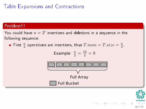
Table Expansions and Contractions
Problem!!!
You could have n = 2t insertions and deletions in a sequence in thefollowing sequence:
First n2 operations are insertions, thus T.num = T.size = n
2 .
Example
Full Array
Full Bucket
66 / 79
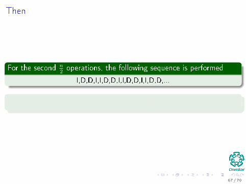
Then
For the second n2operations, the following sequence is performed
I,D,D,I,I,D,D,I,I,D,D,I,I,D,D,...
Thus, the �rst insertion cause a expansion to T.size = n
67 / 79
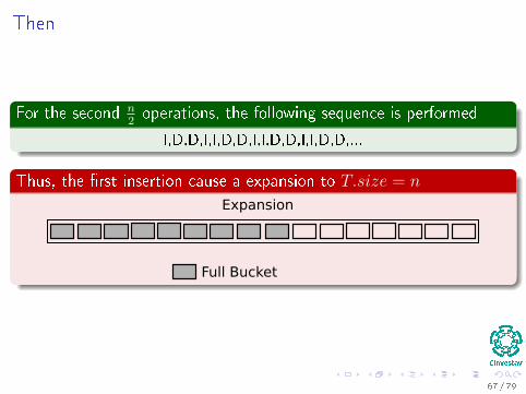
Then
For the second n2operations, the following sequence is performed
I,D,D,I,I,D,D,I,I,D,D,I,I,D,D,...
Thus, the �rst insertion cause a expansion to T.size = n
Expansion
Full Bucket
67 / 79
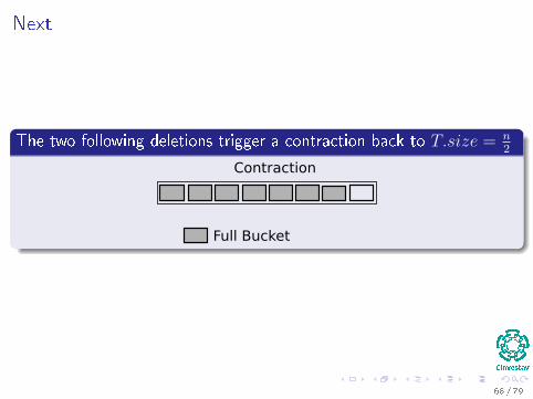
Next
The two following deletions trigger a contraction back to T.size = n2
Contraction
Full Bucket
68 / 79
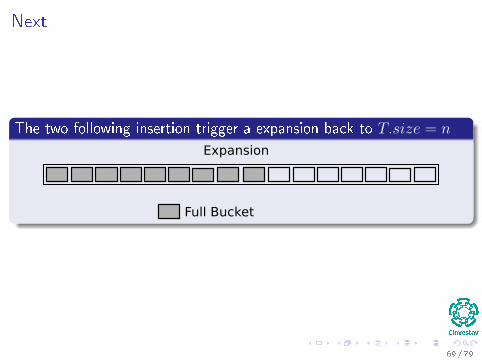
Next
The two following insertion trigger a expansion back to T.size = n
Expansion
Full Bucket
69 / 79
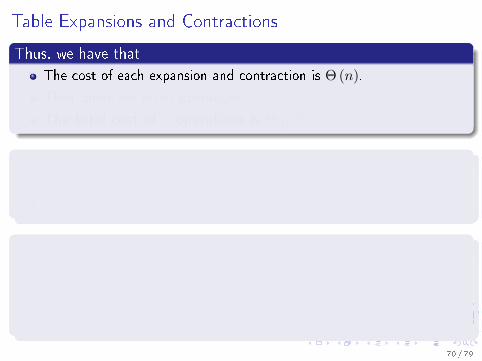
Table Expansions and Contractions
Thus, we have that
The cost of each expansion and contraction is Θ (n).
Then, there are Θ (n) operations.
The total cost of n operations is Θ(n2).
Improvement
You double the table when inserting an item into a full table.
You halve the table when deleting an item makes α (T ) < 14 .
Potential Analysis
Potential Function:
I We require to have a function Φ that is 0 immediately after anexpansion or contradiction.
I Builds potential as the load factors increases to 1 or decreases to 14 .
70 / 79
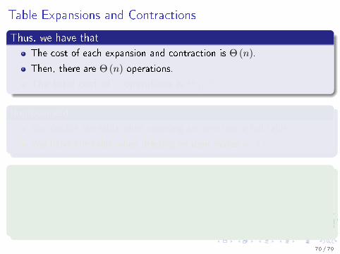
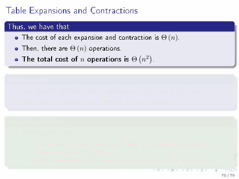
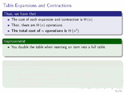
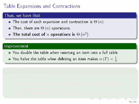
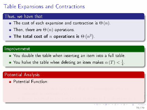
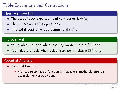
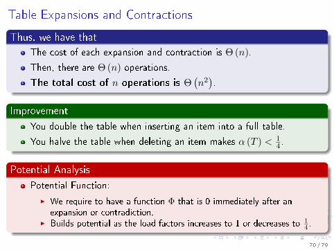
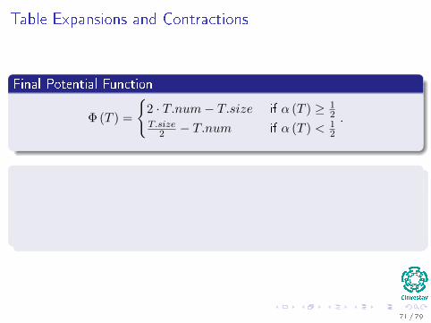
Table Expansions and Contractions
Final Potential Function
Φ (T ) =
{2 · T.num− T.size if α (T ) ≥ 1
2T.size
2 − T.num if α (T ) < 12
.
Properties of this Function
Empty table T.num = T.size = 0, we have that α(T ) = 1.
Then, for an empty or not empty table
I we always have T.num = α (T ) · T.size.
71 / 79
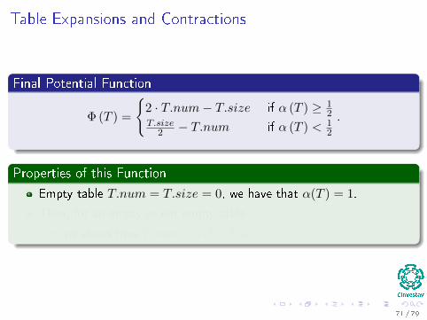
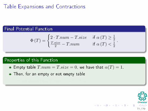
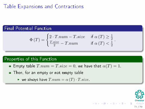
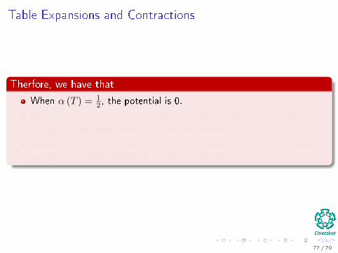
Table Expansions and Contractions
Therfore, we have that
When α (T ) = 12 , the potential is 0.
When α (T ) = 1, we have T.size = T.num⇒ Φ (T ) = T.num. Itcan pay for an expansion, if an item is inserted.
When α (T ) = 14 , we have T.size = 4 · T.num⇒ Φ (T ) = T.num. It
can pay for a contraction, if an item is deleted.
72 / 79
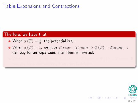
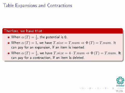
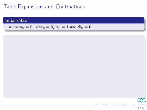
Table Expansions and Contractions
Initialization
num0 = 0, size0 = 0, α0 = 1 and Φ0 = 0.
Case ith operation is a Table-Insert
If αi−1 ≥ 12 , if the table expand or not ci = 3.
If αi <12 , then
ci = ci + Φi − Φi−1
= 1 +
(sizei
2− numi
)−(sizei−1
2− numi−1
)= 1 +
(sizei
2− numi
)−(sizei
2− (numi − 1)
)= 0
73 / 79
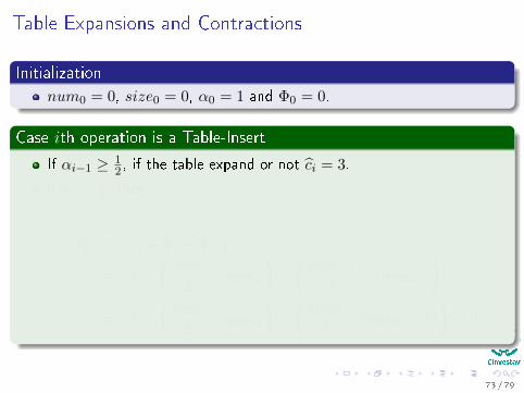
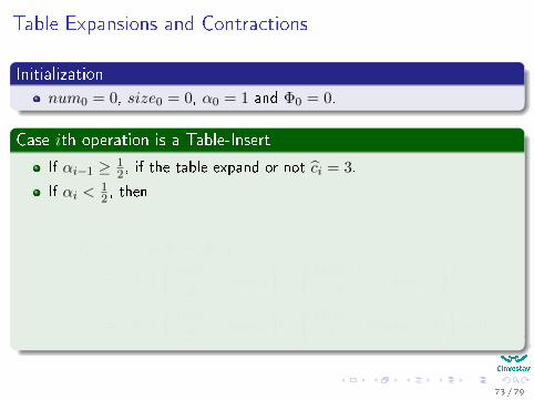
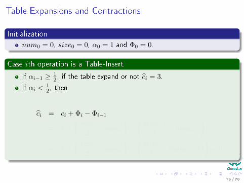
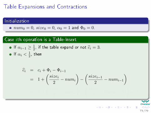
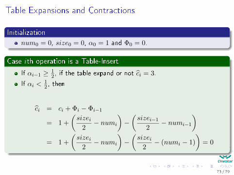
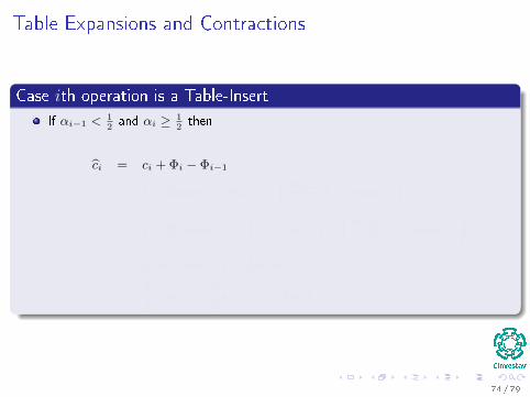
Table Expansions and Contractions
Case ith operation is a Table-Insert
If αi−1 <12and αi ≥ 1
2then
ci = ci + Φi − Φi−1
= 1 + (2numi − sizei) −(sizei−1
2− numi−1
)= 1 + (2 (numi−1 + 1) − sizei−1) −
(sizei−1
2− numi−1
)= 3 · αi−1sizei−1 −
3
2sizei−1 + 3
<3
2sizei−1 −
3
2sizei−1 + 3 = 3
74 / 79
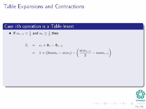
Table Expansions and Contractions
Case ith operation is a Table-Insert
If αi−1 <12and αi ≥ 1
2then
ci = ci + Φi − Φi−1
= 1 + (2numi − sizei) −(sizei−1
2− numi−1
)= 1 + (2 (numi−1 + 1) − sizei−1) −
(sizei−1
2− numi−1
)= 3 · αi−1sizei−1 −
3
2sizei−1 + 3
<3
2sizei−1 −
3
2sizei−1 + 3 = 3
74 / 79

Table Expansions and Contractions
Case ith operation is a Table-Insert
If αi−1 <12and αi ≥ 1
2then
ci = ci + Φi − Φi−1
= 1 + (2numi − sizei) −(sizei−1
2− numi−1
)= 1 + (2 (numi−1 + 1) − sizei−1) −
(sizei−1
2− numi−1
)= 3 · αi−1sizei−1 −
3
2sizei−1 + 3
<3
2sizei−1 −
3
2sizei−1 + 3 = 3
74 / 79
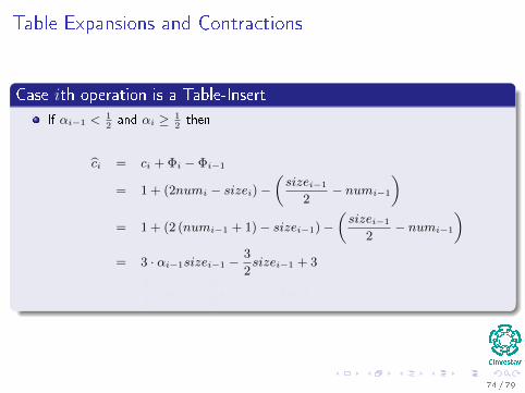
Table Expansions and Contractions
Case ith operation is a Table-Insert
If αi−1 <12and αi ≥ 1
2then
ci = ci + Φi − Φi−1
= 1 + (2numi − sizei) −(sizei−1
2− numi−1
)= 1 + (2 (numi−1 + 1) − sizei−1) −
(sizei−1
2− numi−1
)= 3 · αi−1sizei−1 −
3
2sizei−1 + 3
<3
2sizei−1 −
3
2sizei−1 + 3 = 3
74 / 79
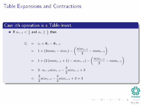
Table Expansions and Contractions
Case ith operation is a Table-Insert
If αi−1 <12and αi ≥ 1
2then
ci = ci + Φi − Φi−1
= 1 + (2numi − sizei) −(sizei−1
2− numi−1
)= 1 + (2 (numi−1 + 1) − sizei−1) −
(sizei−1
2− numi−1
)= 3 · αi−1sizei−1 −
3
2sizei−1 + 3
<3
2sizei−1 −
3
2sizei−1 + 3 = 3
74 / 79
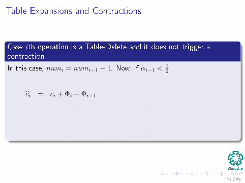
Table Expansions and Contractions
Case ith operation is a Table-Delete and it does not trigger acontraction
In this case, numi = numi−1 − 1. Now, if αi−1 <12
ci = ci + Φi − Φi−1
= 1 +
(sizei
2− numi
)−(sizei−1
2− numi−1
)= 1 +
(sizei
2− numi
)−(sizei−1
2− (numi + 1)
)= 2
75 / 79
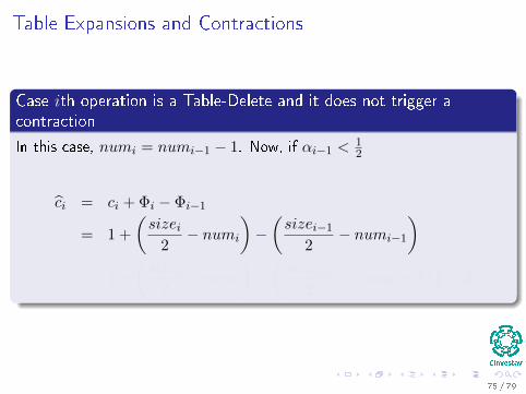
Table Expansions and Contractions
Case ith operation is a Table-Delete and it does not trigger acontraction
In this case, numi = numi−1 − 1. Now, if αi−1 <12
ci = ci + Φi − Φi−1
= 1 +
(sizei
2− numi
)−(sizei−1
2− numi−1
)= 1 +
(sizei
2− numi
)−(sizei−1
2− (numi + 1)
)= 2
75 / 79
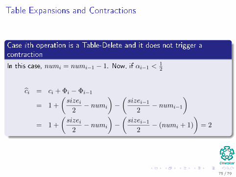
Table Expansions and Contractions
Case ith operation is a Table-Delete and it does not trigger acontraction
In this case, numi = numi−1 − 1. Now, if αi−1 <12
ci = ci + Φi − Φi−1
= 1 +
(sizei
2− numi
)−(sizei−1
2− numi−1
)= 1 +
(sizei
2− numi
)−(sizei−1
2− (numi + 1)
)= 2
75 / 79
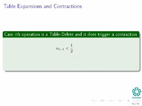
Table Expansions and Contractions
Case ith operation is a Table-Delete and it does trigger a contraction
αi−1 <1
2ci = numi + 1
sizei2
=sizei−1
4= numi−1 = numi + 1
76 / 79

Table Expansions and Contractions
Case ith operation is a Table-Delete and it does trigger a contraction
αi−1 <1
2ci = numi + 1
sizei2
=sizei−1
4= numi−1 = numi + 1
76 / 79
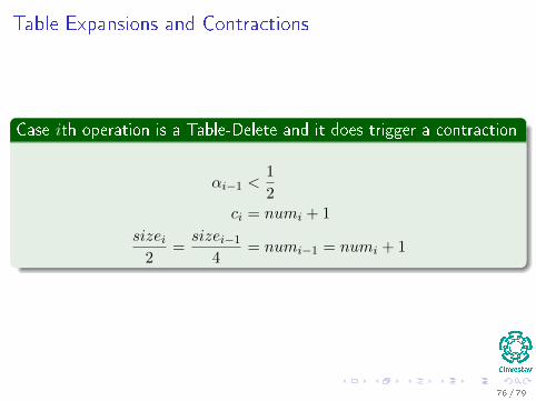
Table Expansions and Contractions
Case ith operation is a Table-Delete and it does trigger a contraction
αi−1 <1
2ci = numi + 1
sizei2
=sizei−1
4= numi−1 = numi + 1
76 / 79
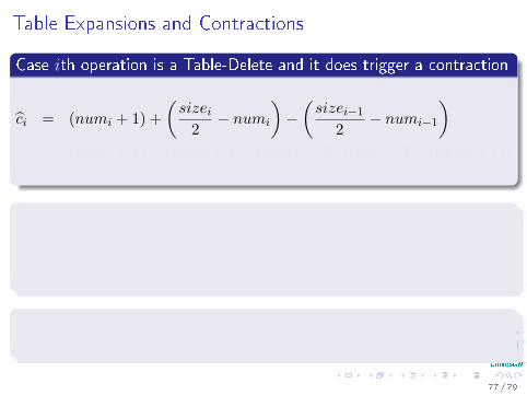
Table Expansions and Contractions
Case ith operation is a Table-Delete and it does trigger a contraction
ci = (numi + 1) +
(sizei
2− numi
)−(sizei−1
2− numi−1
)= (numi + 1) + (numi + 1− numi)− (2 · numi + 2− (numi + 1))
= 1
Case ith operation is a Table-Delete
For αi−1 ≥ 12 .
You can do an analysis and the amortized cost is bounded by aconstant.
Therfore, we have that
The Time for any sequence of n operations on a Dynamic Table is O(n).
77 / 79
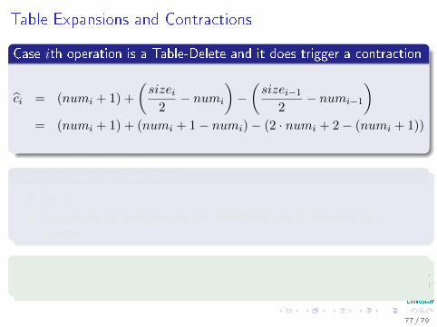
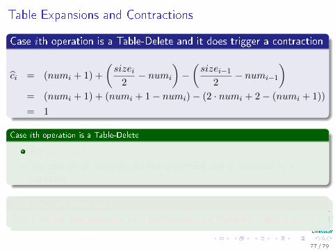
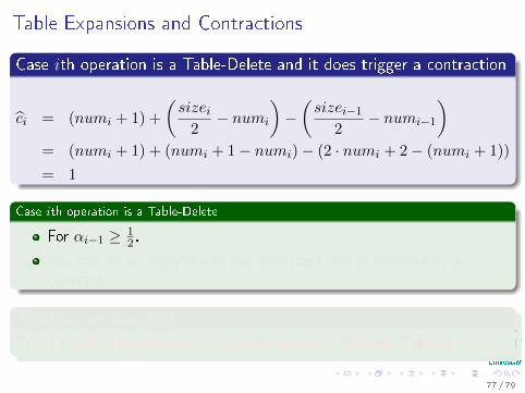
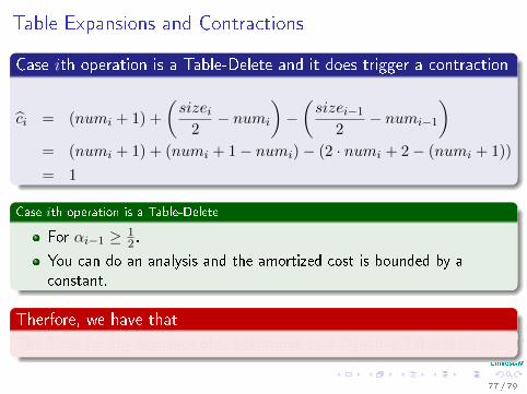
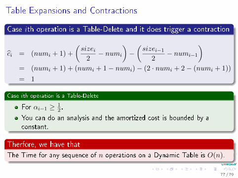
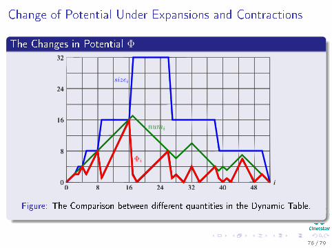
Change of Potential Under Expansions and Contractions
The Changes in Potential Φ
Figure: The Comparison between di�erent quantities in the Dynamic Table.
78 / 79
Exercises
17.1-1
17.1-2
17.1-3
17.2-1
17.2-2
17.2-3
17.3-1
17.3-2
17.3-3
17.3-4
17.3-5
17.3-6
17.3-7
79 / 79