14 artificial intelligence...
TRANSCRIPT

14
Artificial Intelligence Techniques
Si al cabo de tres partidas depoquer no sabes todavıa quien esel tonto, es que el tonto eres tu.
Manuel Vicent
The training program of an ar-tificial intelligence can certainlyinclude an informant, whether ornot children receive negative in-stances.
E. Mark Gold, in [Gol67]
In the different combinatorial methods described in the previous chapters
the main engine to the generalisation process is something like:
‘If nothing tells me not to generalise, do it.’
For example, in the case where we are learning from an informant, the
negative data is providing us with the reason for which one should not
generalise (which is usually performed by merging two states). In the case
of learning from text, the limitations exercised by the extra bias on the
grammar class are what avoids over-generalisation.
But as a principle, the ‘do it if you are allowed’ idea is surely not the
soundest. Since identification in the limit is achieved through elimination
of alternatives, and an alternative can only be eliminated if there are facts
that prohibit it, the principle is mathematically sound but defies common
sense.
There are going to be both advantages and risks to consider a less opti-
mistic point of view, which could be expressed somehow like:
331

332 Artificial Intelligence Techniques
‘If there are good reasons to generalise, then do it.’
On one hand, generalisations will be justified through the fact that there
is some positive ground, some good reason to make them. But on the other
hand we will most often lose the mathematical performance guarantees. It
will then be a matter of expertise to decide if some extra bias has been
added to the system, and then to know if this bias is desired or not.
Let us discuss this point a little further. Suppose the task is learning
Dfa from text, and the algorithm takes as starting point the prefix tree
acceptor, then performs different merges between states whenever this seems
like a good idea. In this case the ‘good idea’ might be something like ‘if it
contributes to diminish the size of the automaton’. Then you will have
added such a heavy bias that your learning algorithm will return always
the universal automaton that recognises any string! Obviously this is a
simple example that would not fool anyone for long. But if we follow on
with the idea, it is not difficult to come up with algorithms whose task is
to learn context-free grammars, but whose construction rules are such that
only grammars that generate regular languages can be effectively learnt!
As, when dealing with these heuristics, the option of identification does
not make sense, it is going to be remarkably difficult to decide when a given
algorithm has such a hidden bias or not.
On the other hand, there are a number of reasons for which researchers in
artificial intelligence have worked thoroughly in searching for new heuristics
for grammatical inference problems:
- The sheer size of the search spaces makes the task of interest. When
describing the set of admissible solutions as a partition lattice (see Sec-
tion 6.3.4), the size of this lattice increased in a dramatic way (defined by
the Bell formula) with the size of the positive data.
- We also saw in Chapter 6 that the basic operations related with the differ-
ent classes of grammars and automata were intractable: the equivalence
problem, the ‘smallest consistent’ problem.
- Furthermore the challenging nature of the associated NP-hard problems
is also something to be taken into account. Even if NP is in theory
a unique class, there are degrees of approximation that can be different
from problem to problem, and it is well known by scientists working on
the effective resolution of NP-hard problems that some can be tackled
easier than others, at least on particular instances, or that the size of
the tractable instances of the problem may vary from one problem to
another. In the case of learning Dfa, the central problem concerns solving

14.1 A survey of some artificial intelligence ideas 333
‘minimum consistent Dfa’, a problem for which only small instances seem
to be tractable by exhaustive algorithms, ‘small’ corresponding to less
than about thirty states in the target.
- A fourth reason is that the point of view we have defended since the begin-
ning, that there is a target language to be found, can in many situations
not be perfectly adapted: In the case where we are given a sample and
the problem is to find the smallest consistent grammar, this corresponds
to trying to solve an intractable but combinatorially well defined prob-
lem; there are finally cases where the data is noisy or where the target is
moving.
The number of possible heuristics is very large, and we will only survey
here some of the main ideas that have been tried in the field.
14.1 A survey of some artificial intelligence ideas
We will comment at the end of the chapter that more techniques could be
tested; indeed one could almost systematically take an artificial intelligence
text-book and choose some meta-heuristic method for solving hard problems,
and then try to adapt it to the task of learning grammars or automata. We
only give the flavour of some of the better studied ideas here. In the next
sections we will describe the use of the following techniques in grammatical
inference:
- genetic algorithms,
- Tabu search,
- using the Mdl principle,
- heuristic greedy search,
- constraint satisfaction.
We aim here to recall the key ideas of the technique and to show, in each case,
through a very brief example, how the technique can be used in grammatical
inference. The goal is certainly not to be technical nor to explain the finer
tuning explanations necessary in practice, but only to give the idea and to
point, in the bibliographical section, to further work with the technique.
14.2 Genetic Algorithms
The principle of genetic algorithms is to simulate biological modifications
of genes and hope that via evolutionary mechanisms, nature increases the
quality of its population. The fact that both bio-computing and grammatical

334 Artificial Intelligence Techniques
inference deal with languages and strings adds a specific flavour to this
approach here.
14.2.1 Genetic algorithms: general approach
Genetic algorithms maintain a population of strings that each encode a
given solution to the learning problem, then by defining the specific genetic
operators allowing this population to evolute and better itself (through an
adequacy to a given fitness function).
In the case where the population is made of grammars or automata sup-
posed to somehow better describe a learning sample, a certain number of
issues should be addressed:
(i) What is the search space? Does it comprise all strings describing
grammars or only those that correspond to correct ones?
(ii) How do we build the first generation?
(iii) What are the genetic operators? Typically some sort of mutation
should exist: A symbol in the string can mutate into another symbol.
Also a crossing-over operator is usually necessary: This operation
takes two strings, mixes them together in some way to obtain the
siblings for the next generation.
(iv) What happens when, after an evolution, the given string does not
encode a solution any more? One may consider having stopping se-
quences in the string so that non-encoding bits can be blocked be-
tween these special sequences. This is quite a nice idea leading to
interesting interpretations about what is known as junk Dna.
(v) What fitness function should be used? How do we compare the qual-
ity of two solutions?
There are also many other parameters that need tuning, such as the num-
ber of generations, the number of elements of a generation that should be
kept, quantities of genetic operations that should take place etc.
Mechanisms of evolution are essentially of two types (gene level): mutation
and crossing-over.
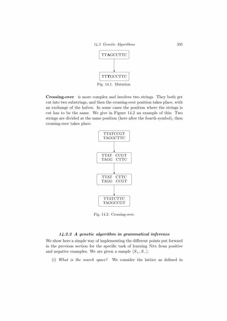
Mutation consists in taking a string and letting one of the letters be mod-
ified. For example, in Figure 14.1, the third symbol is substituted. When
implemented, the operation consists in randomly selecting a position, and
(again randomly) modifying this symbol.
14.2 Genetic Algorithms 335
TTAGCCTTC
TTTGCCTTC
Fig. 14.1. Mutation.
Crossing-over is more complex and involves two strings. They both get
cut into two substrings, and then the crossing-over position takes place, with
an exchange of the halves. In some cases the position where the strings is
cut has to be the same. We give in Figure 14.2 an example of this: Two
strings are divided at the same position (here after the fourth symbol), then
crossing-over takes place.
TTATCCGTTAGGCTTC
TTAT CCGTTAGG CTTC
TTAT CTTCTAGG CCGT
TTATCTTCTAGGCCGT
Fig. 14.2. Crossing-over.
14.2.2 A genetic algorithm in grammatical inference
We show here a simple way of implementing the different points put forward
in the previous section for the specific task of learning Nfa from positive
and negative examples. We are given a sample 〈S+, S−〉.
(i) What is the search space? We consider the lattice as defined in
336 Artificial Intelligence Techniques
Section 6.3, containing all Nfa strongly structurally complete with
〈S+, S−〉. Each Nfa can therefore be represented by a partition of the
states over Mca(S+). There are several ways to represent partitions
as strings. We use the following formalism: let |E| = n, and Π be a
partition, Π = {B1, B2, . . . , Bk} of E. We associate with partition Π
the string wΠ : wΠ(j) = m ⇐⇒ j ∈ Bm.
For example, partition {{1, 2, 6}, {3, 7, 9, 10}, {4, 8, 12}, {5}, {11}}is encoded by the string wΠ=(112341232253).
(ii) How do we generate the first generation? We randomly start from
Mca(S+) (see Definition 6.3.2, page 144), make a certain number of
merges, obtaining in that way a population of Nfa, all in the lattice
and all (weakly) structurally complete.
(iii) What are the genetic operators? Structural operators are structural
mutation and structural crossing-over over the strings wΠ. We illus-
trate this in Example 14.2.1.
(iv) What happens when, after an evolution, the given string does not
encode a grammar any more? This problem does not arise here, as
the operators are built to remain inside the lattice.
(v) What fitness function should be used? Here the two key issues are
the number of strings from S− accepted and the size of the Nfa. We
obviously want both as low as possible. One possibility is even to
discard any Nfa such that L(A) ∩ S− 6= ∅.
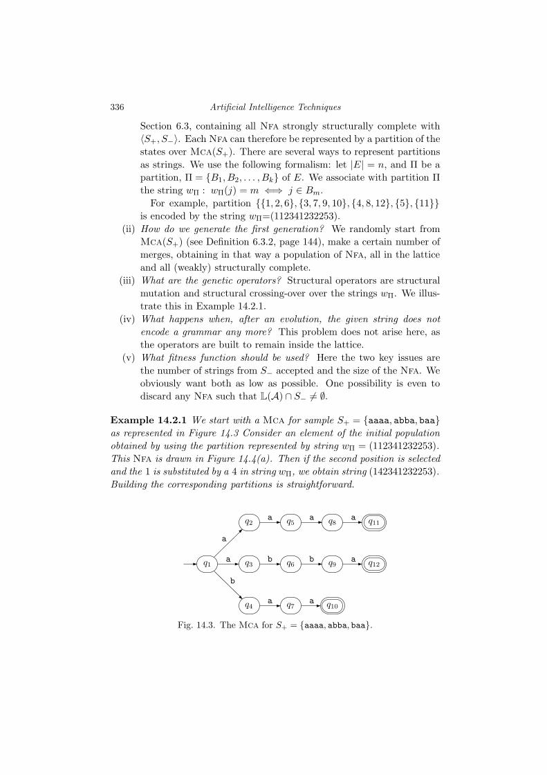
Example 14.2.1 We start with a Mca for sample S+ = {aaaa, abba, baa}as represented in Figure 14.3 Consider an element of the initial population
obtained by using the partition represented by string wΠ = (112341232253).
This Nfa is drawn in Figure 14.4(a). Then if the second position is selected
and the 1 is substituted by a 4 in string wΠ, we obtain string (142341232253).
Building the corresponding partitions is straightforward.
q1
q2
q3
q4
q5
q6
q7
q8
q9
q10
q11
q12
a
a
b
a
b
a
a
b
a
a
a
Fig. 14.3. The Mca for S+ = {aaaa, abba, baa}.

14.2 Genetic Algorithms 337
q1 q2
q3q4
q5
a
a, b
ba
ba
a
aa
a
(a) The Nfa for wΠ =(112341232253).
q1 q2
q3q4
q5
b
ba, b aa
a
a
a a
(b) The Nfa after the muta-tion of 1 to 4 in position 2.
Fig. 14.4. General title.
Now a crossing-over between two partitions is described in Figure 14.5.
The partitions are encoded as strings, which are cut and mixed, resulting in
two different partitions.
{{1, 2, 6}, {3, 7, 9, 10}, {4, 8, 12}, {5}, {11}}{{1, 3, 5}, {2}, {4, 6, 7, 8, 12}, {9, 10, 11}}
(112341232253)(121313334443)
(11234123+2253)(12131333+4443)
(11234123+4443)(12131333+2253)
{{1, 2, 6}, {3, 7}, {4, 8, 12}, {5, 9, 10, 11}}{{1, 3, 5}, {2, 9, 10}, {4, 6, 7, 8, 12}, {11}}
Fig. 14.5. Crossing-over with partitions.

338 Artificial Intelligence Techniques
14.3 Tabu search
When searching in large spaces, hill-climbing techniques try to explore the
space progressively from a starting point to a local optimum, where quality
is measured through a fitness function. As the optimum is only local, to try
to visit further the space, different ideas have been proposed, one of which
corresponds to using Tabu lists, or lists of operations that are forbidden, at
least for a while.
14.3.1 What is Tabu search?
Tabu search also requires the definition of a search space, then the definition
of some local operators to move around this space: Each solution has neigh-
bours and all these neighbours should be measured, the best (for a given
fitness function) being kept for the next iteration. The idea is to iteratively
try to find a neighbour of the current solution, that betters it. In order to
avoid going through the same elements over and over, and getting out of a
local optimum, a Tabu list of the last few moves is kept, and the algorithm
chooses an element outside this list.
There is obviously an issue in reaching a local optimum for the fitness
function. To get out of this situation (i.e. all the neighbours are worse than
the current solution) some sort of major change has to be made.
This sort of heuristic depends strongly on the tuning of a number of
parameters. We will not discuss these here as they require to take into
account a large number of factors (size of the alphabet, the target,. . . ).
14.3.2 A Tabu search algorithm for grammatical inference
The goal is to learn regular languages, defined here by Nfa, from an infor-
mant. An inductive bias is proposed: The number of states in the automaton
(or at least an upper bound of this number) is fixed. The search space is
the set of all Nfa with n states, and the neighbour relation is given by the
fact that from one Nfa to another, the addition or the removal of just one
transition.
(i) What is the search space? The search space is made of λ-Nfa with
n states out of which one (qA) is accepting and all the others are
rejecting. Furthermore qA is reachable by λ-transitions only, and λ-
transitions can only be used for this. There is no transition from qA.
An element in this space is represented in Figure 14.6.
(ii) What are the local operators? Adding and removing a transition.

14.4 Mdl principle in grammatical inference 339
If a transition is added it has to comply with the above rules. For
example, in the automaton represented in Figure 14.6, any of the
transitions could be removed, and transitions could be added con-
necting states q1, q2 and q2, or λ-transitions leading to state qA.
(iii) What fitness function should be used? We count here the number of
strings in S correctly labelled by the Nfa. Function v will therefore
just parse the sample and return the number of errors.
(iv) How do we initialise? In theory, any n state automaton complying
with the imposed rules would be acceptable.
q1
q2
q3
qA
a
b
λ
λ
ab
Fig. 14.6. A Tabu automaton.
We denote by :
- A∗ is the best solution reached so far;
- T is the Tabu list of transitions that have been added or removed in the
last m moves;
- kmax is an integer bounding the number of iterations of the algorithm;
- Q is a set of n− 1 states, qA 6∈ Q is the unique accepting state;
- we denote the rules by triples: R = Q×Σ×Q∪Q×{λ}×{qA}. Therefore
(q, a, q′) ∈ R ⇐⇒ q′ ∈ δN (q, a).
14.4 Mdl principle in grammatical inference
The minimum description length principle states that the best solution is
one that minimises the combination of the encoding of the grammar and the
encoding of the data when parsed by the grammar.
But the principle obeys to some very strict rules. To be more exact the way
both the grammar and the data should be encoded depends on a universal
Turing machine, and has to be handled carefully.

340 Artificial Intelligence Techniques
Algorithm 14.1: Tabu.
Input: a sample S = 〈S+, S−〉, a fitness function v, an integer kmax,
an initial Nfa AOutput: an Nfa
k ← 0;
T ← ∅;
A∗ ← A;
while k 6= kmax dobuild R the set of admissible transitions that can be added or
removed;
select r in R \ T , such that the addition or deletion of r to or from
A realizes the maximum of v on S;
add or delete r from A;
if v(A) > v(A∗) then A∗ ← A;
Tabu-Update(T , r);
k ← k + 1end
return A∗
Algorithm 14.2: Tabu-Update(T , r).
Input: the Tabu list T , its maximal size m, the new element r
Output: T
if card(T ) = m then delete its last element;
Add r as the first element of T ;
return T
14.4.1 What is the Mdl principle?
The Mdl principle is a refinement of the Occam principle: Remember that
the Occam principle tells us that between various hypothesis, one should
choose the simplest. The notion of ‘simplest’ here refers to some fixed no-
tation system. The Mdl principle adds the fact that simplicity should be
measured also in the way the data is explained by the hypothesis. That
means that the simplicity of a hypothesis (with respect to some data S) is
the sum between the size of the encoding of the hypothesis and the size of
the encoding of the data where the encoding of the data can be dependent
of the hypothesis.
As a motivating example take the case of a sample containing strings abaa,
abaaabaa, and abaaabaaabaaabaa. A learning algorithm may come up with

14.4 Mdl principle in grammatical inference 341
either of the two automata depicted in Figure 14.7. Obviously the left-hand
side one (Figure 14.7(a)) is easier to encode than the right-hand side one
(Figure 14.7(b)). But on the other hand the first automaton does not help
us reduce the size of the encoding of the data, whereas using the second
one, the data can easily be encoded as something like {1, 2, 4}, denoting the
number of cycles one should make to generate each string.
qλ
a, b
(a) A very simple Dfa.
qλ
qa
qab
qaba
a b
aa
(b) A more complex one.
Fig. 14.7. Two candidates for sample S+ = {abaa, abaaabaa, abaaabaaabaaabaa}.
14.4.2 A simple Mdl algorithm for grammatical inference
To illustrate these ideas let us try to learn a Dfa from text. We are given
a positive sample S+.
Let us define the score of an automaton as the number of states of the Dfa
multiplied by the size of the alphabet. This is of course questionable, and
should only be considered for a first approach; Since this size is supposed to
be compared with the size of the data, it is essential that the size is fairly
computed. Ideally, the size should be that of the smallest Turing machine
whose output is the automaton. . .
Then, given a string w and a Dfa A, we can encode the string w de-
pending on the number of choices we have at each stage. For example,
using the arguments discussed above for the automata from Figure 14.7,
we just have to encode a string by the numbers of its choices every time
a choice has to be made. We therefore associate with each state of A the
value ch(q)=log(
|{a ∈ Σ : δ(q, a) is defined}|)
if q 6∈ FA. If q ∈ FA then
ch(q)=log(
1 + |{a ∈ Σ : δ(q, a) is defined}|)
, since one more choice is pos-
sible. The value ch corresponds to the size of the encoding of the choices
a parser would have in that state. So in the automaton 14.7(b), we have
ch(qλ)=log 2, ch(qa)=ch(qab)=ch(qaba)=log 1=0. The fact that no cost is
counted corresponds to the idea that no choice has to be made and is also
consistent with log 1 = 0.

342 Artificial Intelligence Techniques
Algorithm 14.3: Mdl.
Input: S+ function Choose
Output: A = 〈Σ, Q, qλ, FA, FR, δ〉A ← Build-PTA(S+);
Red← {qλ};current score ←∞;
Blue← {qa : a ∈ Σ and S+ ∩ aΣ⋆ 6= ∅};while Blue 6= ∅ do
qb ← Choose(Blue);
Blue← Blue \ {qb};if ∃qr ∈ Red : sc(Merge(qr, qb,A),S+)<current score then
A ←Merge(qr, qb,A);
current score ← sc(A,S+)else
A ← Promote(qb,A)
end
end
for qr ∈ Red do
if L(Aqr) ∩ S+ 6= ∅) then FA ← FA ∪ {qr}
end
return A
From this we define the associated value ch(w)=ch(qλ, w) which de-
termines the size of the encoding of the path followed to parse string w,
which depends on the recursive definition: ch(q, λ)= ch(qλ) and ch(q, a ·w)=
ch(q)+ch(δA(q, a), w).
We can now, given a sample S+ and a Dfa A, measure the score sc of A
and S+, (denoted by sc(A, S+)) as ‖A‖ · |Σ| +∑
w∈S+ch(w), where ‖A‖ is
the number of states of A.
We can build a simple state merging algorithm (Algorithm Mdl, 14.3)
which will merge states until it can no longer lower the score. The operations
Merge and Promote are as in Chapter 12.
The training sample is S+ = {a, a2, b2, a3, b2a, a4, ab2a, b4}. From this
we build Pta(S+), depicted in Figure 14.8. We compute the score of the
running solution and we get 13 log(2) + 8 log(3) for the derivations, and 26
for the Pta. The total is therefore sc(A, S+)=39 + 8 log(3) ≈ 51.68.
The exact computations of the ch(x) can be found in Table 14.1.
Merge qa with qλ is tested; This requires recursive merging (for determin-
isation). The resulting automaton is represented in Figure 14.9. The new

14.4 Mdl principle in grammatical inference 343
‖A‖ a a2 b2 a3
12 1+log 3 2+log 3 1+log 3 3+log 3
6 2 log 3 3 log 3 2 log 3 4 log 3
2 2 log 3 3 log 3 2 log 3 4 log 3
1 2 3 3 4
‖A‖ b2a a4 ab2a b4
12 1+log 3 3+log 3 1+log 3 1+log 3
6 2 log 3 5 log 3 3 log 3 2 log 3
2 3 log 3 5 log 3 4 log 3 3 log 3
1 4 5 5 5
Table 14.1. Computations of all the ch(x), for the Pta and the different
automata
qλ
qa
qb
qa2
qab
qb2
qa3
qab2
qb2a
qb3
qa4
qab2a
qb3
a
b
a
b
b
a
b
a
bb
a
a
Fig. 14.8. Pta(S+) where S+ = {a, a2, b2, a3, b2a, a4, ab2a, b4}.
automaton has values ch(qλ)=ch(qb2)=log 3, and ch(qb)=ch(q
b2a)=ch(q
b3)=
ch(qb4)=log 1=0. So sc(A, S+) can be computed as:
6 · 2 + 23 log(3) < 36 + 11 log(3) (roughly 48.45 against 51.68), the merge
is accepted.
qλ qb qb2
qb2a
qb3 qb4
a
bb
a
bb
Fig. 14.9. We merge qa with qλ.
We try to merge qb with qλ and obtain the universal automaton whose
score is 2 for the Dfa + 31 log(3). This gives a score of 51.13, which is

344 Artificial Intelligence Techniques
more than the score of our current solution (with 6 states). Therefore the
merge is rejected. qb is promoted and we test merging qab with qλ. After
determinisations we obtain the 2 state automaton depicted in Figure 14.10.
The score of this Dfa is 43.68, which is better than the current best. Since
no more merges are possible the algorithm halts with this Dfa as solution.
qλ qb
a
b
b
Fig. 14.10. The returned solution.
Note that by taking a different scoring scheme, the result would have been
very different (see Exercises 14.7 and 14.8).
14.5 Heuristic Greedy State Merging
When we described Rpni (Section 12.4), we presented it as a deterministic
algorithm. Basically, the order in which the compatibilities are checked is
defined right from the start. Moreover, as soon as two states are mergeable
these are merged. This is clearly an optimistic point of view, and there may
be another, based on choosing the best merge.
But one should remember that Rpni identifies in the limit. This may well
no longer be the case if we use a heuristic to define the best possible merge:
One can usually imagine a (luckily counter-intuitive) distribution that will
make us explore the lattice the wrong way.
14.5.1 How do greedy state merging algorithms work?
The general idea of a greedy state merging algorithm is as follows:
- choose two states,
- perform a cascade of forced merges until the automaton is deterministic,
- if this automaton accepts some sentences from S−, backtrack and choose
another couple,
- if not, loop until no merging is still possible.
Now how are the moves chosen? Consider the current automaton for
which Rpni has to make a decision: What moves are allowed?
There are two possibilities:
14.5 Heuristic Greedy State Merging 345
- merging a Blue with a Red,
- promoting a Blue to Red and changing all its successors that are not
Red to Blue.
Promotion takes place when a Blue state can be merged with no Red
state. This means that this event (similar to having a row obviously different
in Gold’s algorithm) has to be systematically checked.
But once there are no possible promotions, the idea is to do better than
Rpni and, instead of greedily checking in order to find the first admissible
merge, to check all possible legal merges between a Blue state and a Red
state, compute a score for each merge, and then choose the merge with
highest score.
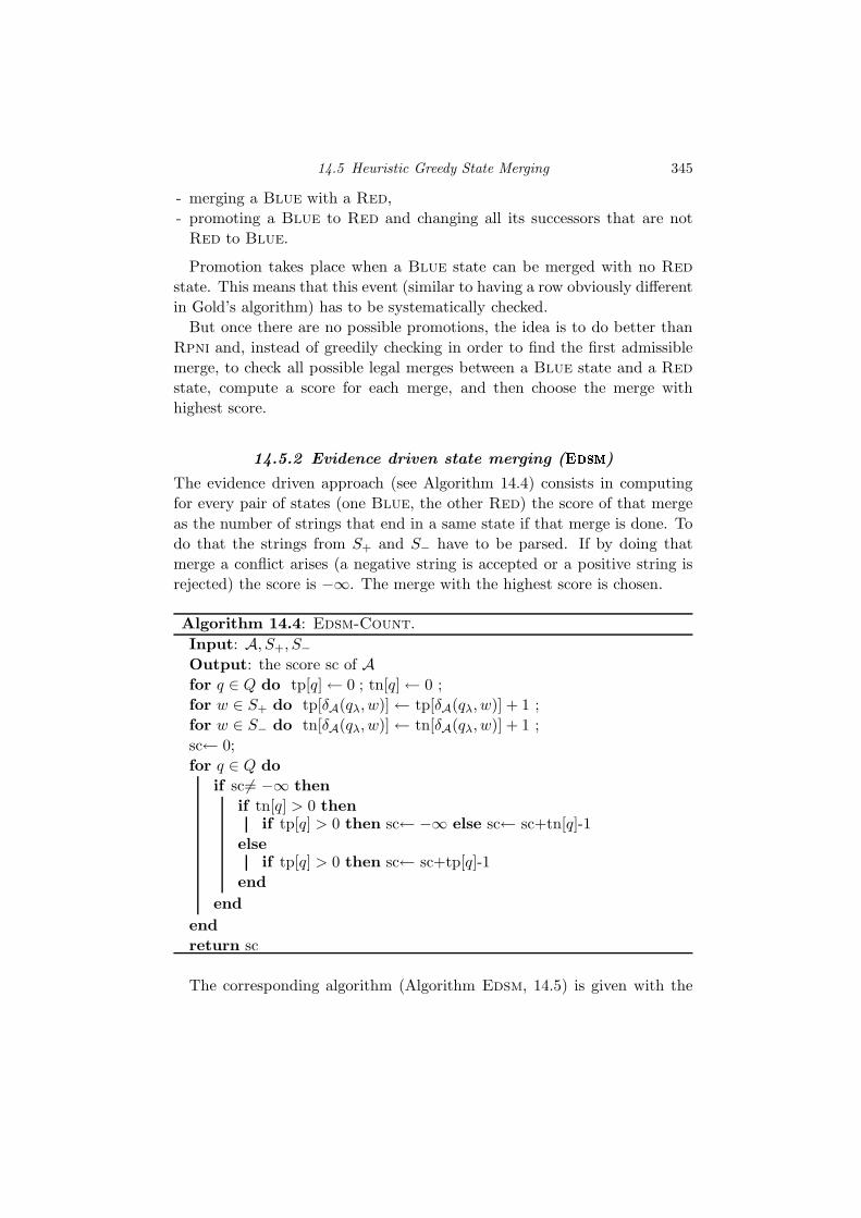
14.5.2 Evidence driven state merging (Edsm)
The evidence driven approach (see Algorithm 14.4) consists in computing
for every pair of states (one Blue, the other Red) the score of that merge
as the number of strings that end in a same state if that merge is done. To
do that the strings from S+ and S− have to be parsed. If by doing that
merge a conflict arises (a negative string is accepted or a positive string is
rejected) the score is −∞. The merge with the highest score is chosen.
Algorithm 14.4: Edsm-Count.
Input: A, S+, S−
Output: the score sc of Afor q ∈ Q do tp[q]← 0 ; tn[q]← 0 ;
for w ∈ S+ do tp[δA(qλ, w)]← tp[δA(qλ, w)] + 1 ;
for w ∈ S− do tn[δA(qλ, w)]← tn[δA(qλ, w)] + 1 ;
sc← 0;
for q ∈ Q do
if sc6= −∞ then
if tn[q] > 0 then
if tp[q] > 0 then sc← −∞ else sc← sc+tn[q]-1
else
if tp[q] > 0 then sc← sc+tp[q]-1
end
end
end
return sc
The corresponding algorithm (Algorithm Edsm, 14.5) is given with the

346 Artificial Intelligence Techniques
specific counting scheme (Algorithm Edsm-Count, 14.4). The merging
function is exactly the one (Algorithm 12.11) introduced in Section 12.4.
Algorithm 14.5: Edsm A.
Input: S = 〈S+, S−〉, functions Compatible, Choose
Output: A = 〈Σ, Q, qλ, FA, FR, δ〉A ← Build-Pta(S+); Red← {qλ}; Blue← {qa : a ∈ Σ and
S+ ∩ aΣ⋆ 6= ∅};
while Blue 6= ∅ dopromotion← false;
for qb ∈ Blue do
if not promotion thenbs← −∞;
atleastonemerge← false;
for qr ∈ Red do
s←Edsm-Count(Merge(qr, qb,A),S+, S− );
if s > −∞ then atleastonemerge← true
if s > bs then bs← s; qr ← qr; qb ← qb
end
if not atleastonemerge then /* no merge is possible */Promote(qb,A); promotion← true;
end
end
end
if not promotion then /* we can merge */Blue← Blue \ {qb}; A ←Merge(qr, qb,A)
end
end
for x ∈ S+ do FA ← FA ∪ {δ(qλ, x)};for x ∈ S− do FR ← FR ∪ {δ(qλ, x)};
return A
Example 14.5.1
S+ = {a, aaa, bba, abab}
S− = {ab, bb}
Consider the Dfa represented in Figure 14.11. States qλ and qa are Red,
whereas states qb and qab are Blue. We compute the different scores for the
sample, if we suppose that the Blue state selected for merging is qb:

14.5 Heuristic Greedy State Merging 347
In both cases the merge is actually tested, and counting (via Algorithm
Edsm-Count (14.4) is done.
S+ = {a, aaa, aba, bba, abab}
S− = {ab, bb}
State qab is now selected and the counts are computed:
qλ
qa
aa
qbb
qab
b
qbb
b
qabaa
qbbaa
qabab
b
Fig. 14.11. The Dfa before attempting a merge.
• Edsm-Count(Merge(qλ, qab,A))=−∞, because this consists in merg-
ing qab with qabab.
• Edsm-Count(Merge(qa, qab,A))=−∞, because this consists in merg-
ing qa with qab.
Therefore a promotion takes place: Since we have a Blue which can be
merged, the Dfa is updated with state qab promoted to Red (see Figure
14.12).
qλ
qa
aa
qbb
qab
b
qbb
b
qabaa
qbbaa
qabab
b
Fig. 14.12. The Dfa after the promotion of qab.
Suppose instead state b was selected. The counts are now different
• Edsm-Count(Merge(qλ, qb,A))=2
• Edsm-Count(Merge(qa, qb,A))=3
In this case, the merge between qa and qb would be selected.

348 Artificial Intelligence Techniques
There are different ways to perform the possible operations but what
characterises the evidence driven state merging techniques is that one should
be careful to always check first if some promotion is possible.
A different idea is to use a heuristic to decide before testing consistency
in what order the merges should be checked. This is of course cheaper,
but the problem is that promotion is then hard to detect. In practice this
approach (called data driven) has not proven to be successful, at least in
the deterministic setting. When trying to learn probabilistic automata, it
seems that data driven state merging is a good option.
14.6 Graph colouring and constraint satisfaction
The Pta can be seen as a graph for which the goal is to obtain a colouring
of the nodes respecting a certain number of conditions. These conditions
can be described as constraints, and again the nodes of the graph have to
be valued in a way satisfying a set of constraints. Alas these constraints are
dynamic (some constraints will depend on others).
There are too many options to mention them all here, we just describe
briefly how we can convert the problem of learning a Dfa from an informed
sample 〈S+, S−〉 into a constraint satisfaction question.
We first build the complete prefix tree acceptor Pta(S+, S−) using Algo-
rithm 12.1, page 281. Let us suppose the Pta has m states.
Now consider the graph whose nodes are the states of the Pta and where
there is an edge between two nodes/states q and q′ if they are incompatible,
i.e. they cannot be merged. Then the problem is to find a colouring of the
graph (no two adjacent nodes can take the same colour) with a minimum
number of colours.
An alternative problem whose resolution can provide us with a partition
is that of building cliques in the graph of consistency.
Technically things are a little more complex, since the constraints are
dynamic: Choosing to colour two nodes with a given colour corresponds to
merging the states, with the usual problems relating to determinism.
Nevertheless there are many heuristics that have been tested for these
particular and well known problems.
Let us model further the problem. We consider (given the Pta) m vari-
ables X1, . . . ,Xm, and n possible values 1,. . . , n, corresponding to the n
states of the target automaton (which supposes we take an initial gamble
on the size of the intended target).
One can describe three types of constraints:

14.7 Exercises 349
- global constraints: qi ∈ FA, qj ∈ FR =⇒ Xi 6= Xj ;
- propagation constraints: Xk 6= Xl∧ δ(qi, a) = qk∧ δ(qj , a) = ql =⇒ Xi 6=Xj ;
- deterministic constraints: δ(qi, a) = qj ∧ δ(qk, a) = ql =⇒[
Xi = Xk =⇒Xj = Xl
]
.
Note that the deterministic constraints are dynamic: They will only be
used when the algorithm starts deciding to effectively colour some states.
Between the different systems used to solve such constraints, conflict di-
agnosis (using intelligent backtracking) has been used.
Example 14.6.1 Consider the Pta represented in Figure 14.13. Then a
qλ
qa
qb
qaa
qab
qbb
qaba
qbba
qabab
a
b
a
b
b
a b
a
Fig. 14.13. Pta({(aa, 1) (aba, 0) (bba, 1) (ab, 0) (abab, 1)}).
certain number of initial global constraints can be established. If we denote
by 〈Xi,Xj〉 the constraint: “qi and qj cannot be merged”, we have by taking
all pairs of states, one being accepting and the other rejecting:
Initial constraints: 〈Xaa,Xab〉, 〈Xaa,Xaba〉, 〈Xabab,Xab〉, 〈Xabab,Xaba〉,〈Xbba,Xab〉, 〈Xbba,Xaba〉.
We can now represent some of the propagation constraints, where we use
the rule 〈Xua,Xva〉 =⇒ 〈Xu,Xv〉.
〈Xua,Xva〉 =⇒ 〈Xu,Xv〉
This, when propagated, gives us 〈Xa,Xab〉, 〈Xab,Xbb〉, 〈Xa,Xb〉, 〈Xa, qaba〉,
〈Xλ,Xab〉.
14.7 Exercises
14.1 Write the different missing algorithms for the genetic algorithms.
14.2 Find a difficult language to identify with a genetic algorithm.
14.3 The definition of the value function v for the Tabu search method is
very naive. Can we do better?
14.4 Find a difficult language to identify with the Tabu search algorithm,
using a fixed k.

350 Artificial Intelligence Techniques
14.5 If the target is a complete automaton, then the Mdl algorithm will
perform poorly. Why?
14.6 What would be a good class of Dfa that for the Mdl algorithm?
Hint: one may want to have large alphabets but only very few tran-
sitions. A definition in the spirit of Definition 4.4.1 (page 96 may be
a good idea.
14.7 Using the same data as in Section 14.4, run the Mdl algorithm
with a score function that ignores the size of the alphabet, i.e.
sc(A, S+))=‖A‖+∑
w∈S+ch(w).
14.8 Conversely, let us suppose we intend to represent the automaton as a
table with three entries (one for the alphabet and two for the states).
Therefore we could choose sc(A, S+))=‖A‖2 · |Σ|+∑
w∈S+ch(w)
14.9 In Algorithm Edsm, the computation of the scores is very expensive.
Can we combine the data driven and the evidence driven approaches
in order to not have to compute all the scores but to be able to
discover the promotion situations?
14.10 In Algorithm Edsm, once sc(q,q′,A) is computed as −∞, does it
need to be recomputed? Is there any way to avoid such expensive
recomputations?
14.11 Build the set of constraints corresponding to the Pta represented in
Figure 14.14
qλ
qa
qb
qaa
qab
qbb
qaab
qbba
qabab
a
b
a
b
b
a
b
a
Fig. 14.14. Pta({(aa, 1) (aab, 0) (bba, 0) (ab, 0) (abab, 1)}).
14.8 Conclusions of the chapter and further reading
14.8.1 Bibliographical background
Some of the key ideas presented in the first section of this chapter have been
discussed in [dlH06a].
The question of the size of the Dfa is a real issue. Whereas following
on the line of the Abbadingo competition [LP97], many authors were keen
on finding algorithms working with targets of a few hundred states, there

14.8 Conclusions of the chapter and further reading 351
has been also a group of researchers intersected in considering the purely
combinatoric problem of finding the smallest Dfa and coming up with some
heuristics for this case [dOS01].
Presentation of Section 14.2 on genetic algorithms is based on work by
many researchers but specially [Dup94, SK99, SM00]. Research in this area
has taken place both from the grammatical inference perspective and from
the genetic algorithms one. It is therefore essential, when wanting to study
this particular topic, to look at the bibliography from both areas. An at-
tempts to use genetic algorithms (using the term coevolutionary learning)
in an active setting was made by Josh Bongard and Hod Lipson [BL05].
The Mdl principle is known under different names [WB68, Ris78]. In
grammatical inference some key ideas were introduced by Gerard Wolff
[Wol78]. More recently his work was pursued by Pat Langley and Sean
Stromstean [Lan95, LS00], George Petasis et al.[PPK+04]. New ideas, in
the case of learning Dfa with Mdl are by Pieter Adriaans and Ceriel Ja-
cobs [AJ06].
Presentation of Section 14.3, concerning Tabu search, is based on work by
Jean-Yves Giordano [Gio96]. A more general presentation of Tabu search,
can be found in Fred Glover’s book [GL97].
The main results concerning algorithm Edsm correspond to work done by
Nick Price, Hugues Juille and Kevin Lang during or after the Abbadingo
competition [LPP98, Lan99]. The cheaper (but also worse) data driven
approach was used by Colin de la Higuera et al. [dlHOV96]
Presentation of Section 14.6 is based on work by Alan Biermann [Bie71],
Arlindo de Oliveira and Joao Marques Silva[dOS98], Francois Coste [CN98b,
CN98a].
Pure heuristics are problematic in that they can introduce an unwanted,
undeclared added bias. Typically if the intended class of grammars is dif-
ferent from the one that is really going to be learnt, something is wrong.
An interesting alternative is to base a heuristic on a provably convergent
algorithm. There is still the necessity to study what is really happening in
this case, but a prudent guess is that somehow one is keeping control of the
bias.
14.8.2 Some alternative lines of research
- A very different approach to learn context-free grammars has been fol-
lowed in system Synapse by Katsuhiko Nakamura and his colleagues
[NM05]: The goal there is to learn directly and inductively the Cky
parser. The system is in part incremental. Along similar lines have

352 Artificial Intelligence Techniques
been tried genetic algorithms, with the same goal of learning the parser
[SK99, SM00].
- Neural networks have been used in grammatical inference with varying
degrees of success. Among the best known papers are those by Rene
Alquezar and Alberto Sanfeliu, Lee Giles, Mikel Forcada, and their col-
leagues [AS94, CFS96, GLT01]. In some cases a mixture of numerical
and symbolic techniques were used: The symbolic grammatical inference
allowing to better find the parameters for the recurrent network and con-
versely the network allowing to decide compatibility of states. An im-
portant question is that of extracting an automaton from a learnt neural
network, so as to avoid the black-box effect. In this case, we can be facing
an interesting task of interactive learning in which the neural network can
play the part of the Oracle.
14.8.3 Open problems and possible new lines of research
There is obviously a lot of work possible, once the limits of provable meth-
ods are well understood. Let us discuss a certain number of elements of
reflection:
- The Gold algorithm gives an interesting basis for learning as it redefines
the search space. This should be considered as a good place to start from.
Moreover, the complexity of the algorithm can be considerably reduced
through a careful use of good data structures.
- Use of semantic information in real tasks should be encouraged. This
semantic information needs to be translated into syntactic constraints
that in turn could improve the algorithms.
- Edsm is a good example of what should be done: The basis is a provable
algorithm (Rpni) in which the greediness is controlled by a common sense
function instead of by an arbitrary order.