1482 ieee transactions on pattern analysis and … · voting (cftv), which is applicable to the...

A Closed-Form Solution to Tensor Voting:Theory and Applications

Tai-Pang Wu, Member, IEEE Computer Society, Sai-Kit Yeung, Member, IEEE Computer Society,

Jiaya Jia, Senior Member, IEEE, Chi-Keung Tang, Senior Member, IEEE, and

Gerard Medioni, Fellow, IEEE

Abstract—We prove a closed-form solution to tensor voting (CFTV): Given a point set in any dimensions, our closed-form solution

provides an exact, continuous, and efficient algorithm for computing a structure-aware tensor that simultaneously achieves salient

structure detection and outlier attenuation. Using CFTV, we prove the convergence of tensor voting on a Markov random field (MRF),

thus termed as MRFTV, where the structure-aware tensor at each input site reaches a stationary state upon convergence in structure

propagation. We then embed structure-aware tensor into expectation maximization (EM) for optimizing a single linear structure to

achieve efficient and robust parameter estimation. Specifically, our EMTV algorithm optimizes both the tensor and fitting parameters

and does not require random sampling consensus typically used in existing robust statistical techniques. We performed quantitative

evaluation on its accuracy and robustness, showing that EMTV performs better than the original TV and other state-of-the-art

techniques in fundamental matrix estimation for multiview stereo matching. The extensions of CFTV and EMTV for extracting multiple

and nonlinear structures are underway.

Index Terms—Tensor voting, closed-form solution, structure inference, parameter estimation, multiview stereo.

Ç

1 INTRODUCTION

THIS paper reinvents tensor voting (TV) [19] for robustcomputer vision by proving a closed-form solution to

computing an exact structure-aware tensor after data commu-nication in a feature space of any dimensions, where the goalis salient structure inference from noisy and corrupted data.

To infer structures from noisy data corrupted by outliers,in tensor voting, input points communicate among them-selves subject to proximity and continuity constraints.Consequently, each point is aware of its structure saliencyvia a structure-aware tensor. Structure refers to surfaces,curves, or junctions if the feature space is three dimensionalwhere a structure-aware tensor can be visualized as anellipsoid: If a point belongs to a smooth surface, theresulting ellipsoid after data communication resembles a

stick pointing along the surface normal; if a point lies on acurve the tensor resembles a plate where the curve tangentis perpendicular to the plate tensor; if it is a point junctionwhere surfaces intersect, the tensor will be like a ball. Anoutlier is characterized by a set of inconsistent votes itreceives after data communication.

We develop in this paper a closed-form solution to tensorvoting (CFTV), which is applicable to the special as well asgeneral theory of tensor voting. This paper focuses on thespecial theory, where the above data communication is datadriven without using constraints other than proximity andcontinuity. The special theory, sometimes coined “first votingpass,” is applied to process raw input data to detect structuresand outliers. In addition to structure detection and outlierattenuation, in the general theory of tensor voting tensor votesare propagated along preferred directions to achieve datacommunication when such directions are available, typicallyafter the first pass, such that useful tensor votes arereinforced, whereas irrelevant ones are suppressed.

Expressing tensor voting in a single and compact equa-tion, or a closed-form solution, offers many advantages: Notonly can an exact and efficient solution be achieved with lessimplementation effort for salient structure detection andoutlier attenuation, formal and useful mathematical opera-tions such as differential calculus can be applied, which isotherwise impossible using the original tensor votingprocedure. Notably, we can prove the convergence of tensorvoting on Markov random fields (MRFTV), where astructure-aware tensor at each input site achieves a stationarystate upon convergence.

Using CFTV, we contribute a mathematical derivationbased on expectation maximization (EM) that applies theexact tensor solution for extracting the most salient linearstructure, despite the fact that the input data are highlycorrupted. Our algorithm is called EMTV, which optimizes

1482 IEEE TRANSACTIONS ON PATTERN ANALYSIS AND MACHINE INTELLIGENCE, VOL. 34, NO. 8, AUGUST 2012

. T.-P. Wu is with the Enterprise and Consumer Electronics (ECE) Group,Hong Kong Applied Science and Technology Research Institute (ASTRI)Co. Ltd., 3/F, Bio-informatics Centre, 2 Science Park West Avenue, HongKong Science Park, Shatin, Hong Kong. E-mail: [email protected].

. S.-K. Yeung is with the Pillar of Information Systems Technology andDesign, The Singapore University of Technology and Design, 20 DoverDrive, Singapore 128805. E-mail: [email protected].

. J. Jia is with the Department of Computer Science and Engineering, TheChinese University of Hong Kong, Shatin, Hong Kong.E-mail: [email protected].

. C.-K. Tang is with the Department of Computer Science and Engineering,The Hong Kong University of Science and Technology, Clear Water Bay,Hong Kong. E-mail: [email protected].

. G. Medioni is with the Institute for Robotics and Intelligent Systems,University of Southern California, PHE 204, MC-2073, Los Angeles, CA90089-0273. E-mail: [email protected].

Manuscript received 13 July 2010; revised 31 Jan. 2011; accepted 6 Nov. 2011;published online 13 Dec. 2011.Recommended for acceptance by C. Stewart.For information on obtaining reprints of this article, please send e-mail to:[email protected], and reference IEEECS Log NumberTPAMI-2010-07-0529.Digital Object Identifier no. 10.1109/TPAMI.2011.250.

0162-8828/12/$31.00 � 2012 IEEE Published by the IEEE Computer Society

both the tensor and fitting parameters upon convergenceand does not require random sampling consensus(RANSAC) typical of existing robust statistical techniques.The extension to extract salient multiple and nonlinearstructures is underway.

While the mathematical derivation may seem involved,our main results for CFTV, MRFTV, and EMTV, that is, (11),(12), (18), (19), (26), and (30), have rigorous mathematicalfoundations, are applicable to any dimensions, producemore robust and accurate results, as demonstrated in ourqualitative and quantitative evaluation using challengingsynthetic and real data, but, on the other hand, are easier toimplement. The source codes accompanying this paper areavailable in the supplemental material, which can be foundiat http://www.cs.ust.hi/!cktang/tv_code.zip.

2 RELATED WORK

While this paper is mainly concerned with tensor voting,we provide a concise review on robust estimation andexpectation maximization.

Robust estimators. Robust techniques are widely usedand an excellent review of the theoretical foundations ofrobust methods in the context of computer vision can befound in [20].

The Hough transform [13] is a robust voting-basedtechnique operating in a parameter space capable ofextracting multiple models from noisy data. StatisticalHough transform [6] can be used for high-dimensionalspaces with sparse observations. Mean shift [5] has beenwidely used since its introduction to computer vision forrobust feature space analysis. The Adaptive Mean Shift [11]with variable bandwidth in high dimensions was intro-duced in texture classification and has since been applied toother vision tasks. Another popular robust method incomputer vision is in the class of random samplingconsensus procedures [7], which have spawned a lot offollow-up work (e.g., optimal randomized RANSAC [4]).

Like RANSAC [7], robust estimators, including theLMedS [22] and the M-estimator [14], adopted a statisticalapproach. The LMedS, RANSAC, and the Hough transformcan be expressed as M-estimators with auxiliary scale [20].The choice of scales and parameters related to the noiselevel are major issues. Existing works on robust scaleestimation use random sampling [26] or operate ondifferent assumptions (e.g., more than 50 percent of thedata should be inliers [23]; inliers have a Gaussiandistribution [15]). Among them, the Adaptive Scale SampleConsensus (ASSC) estimator [28] has shown the bestperformance where the estimation process requires no free

parameter as input. Rather than using a Gaussian distribu-tion to model inliers, the authors of [28] proposed to use atwo-step scale estimator (TSSE) to refine the model scale:First, a non-Gaussian distribution is used to model inlierswhere local peaks of density are found by mean shift [5];second, the scale parameter is estimated by a median scaleestimator with the estimated peaks and valleys. On theother hand, the projection-based M-estimator (pbM) [3], animprovement made on the M-estimator, uses a Parzenwindow for scale estimation, so the scale parameter isautomatically found by searching for the normal direction(projection direction) that maximizes the sharpest peak ofthe density. This does not require an input scale from theuser. While these recent methods can tolerate more outliers,most of them still rely on or are based on RANSAC and anumber of random sampling trials is required to achieve thedesired robustness.

To reject outliers, a multipass method using L1-normswas proposed to successively detect outliers which arecharacterized by maximum errors [24].

Expectation maximization. EM has been used in hand-ling missing data and identifying outliers in robustcomputer vision [8], and its convergence properties werestudied [18]. In essence, EM consists of two steps [2], [18]:

1. E-Step. Computing an expected value for thecomplete data set using incomplete data and thecurrent estimates of the parameters.

2. M-Step. Maximizing the complete data log likelihoodusing the expected value computed in the E-step.

EM is a powerful inference algorithm, but it is also wellknown from [8] that: 1) Initialization is an issue because EMcan get stuck in poor local minima, and 2) treatment of datapoints with small expected weights requires great care.They should not be regarded as negligible, as theiraggregate effect can be quite significant. In this paper, weinitialize EMTV using structure-aware tensors obtained byCFTV. As we will demonstrate, such initialization not onlyallows the EMTV algorithm to converge quickly (typicallywithin 20 iterations) but also produces accurate and robustsolution in parameter estimation and outlier rejection.

3 DATA COMMUNICATION

In the tensor voting framework, a data point, or voter,communicates with another data point, or vote receiver,subject to proximity and continuity constraints, resulting ina tensor vote cast from the voter to the vote receiver (Fig. 1).In the following, we use n to denote a unit voting sticktensor, v to denote a stick tensor vote received. Stick tensor

WU ET AL.: A CLOSED-FORM SOLUTION TO TENSOR VOTING: THEORY AND APPLICATIONS 1483

Fig. 1. Inlier/outlier and tensor inverse illustration. (a) The normal votes received at a surface point cast by points in x’s neighborhood. Three salientoutliers are present. (b) For a nonsurface point, there is no preference to any normals. (c) The structure-aware tensor induced by the normalobservations in (a), which is represented by a d-D ellipsoid, where d � 2. The orange curve (dashed curve) represents the variance produced alongall possible directions. (d) The structure-aware tensor collected after collecting the received votes in (b). (e) and (f) correspond to the inverse of(c) and (d), respectively.

vote may not be unit vectors when they are multiplied byvote strength. These stick tensors are building elements of astructure-aware tensor vote.

Here, we first define a decay function � to encode theproximity and smoothness constraints ((1) and (2)). Whilesimilar in effect to the decay function used in the originaltensor voting and also to the one used in [9], where avote attenuation function is defined to decouple proximityand curvature terms, our modified function, which alsodiffers from that in [21], enables a closed-form solutionfor tensor voting without resorting to precomputeddiscrete voting fields.

Refer to Fig. 2. Consider two points xi 2 IRd and xj 2 IRd

(where d > 1 is the dimension) that are connected by somesmooth structure in the feature/solution space. Supposethat the unit normal nj at xj is known. We want to generateat xi a normal (vote) vi so that we can calculate Ki 2IRd � IRd, where Ki is the structure-aware tensor at xi inthe presence of nj at xj. In tensor voting, a structure-awaretensor is a second-order symmetric tensor, which can bevisualized as an ellipsoid.

While many possibilities exist, the unit direction vi canbe derived by fitting an arc of the osculating circle betweenthe two points. Such an arc keeps the curvature constantalong the hypothesized connection, thus encoding thesmoothness constraint. Ki is then given by viv

Ti multiplied

by �ðxi;xj;njÞ defined as

�ðxi;xj;njÞ ¼ cij�1�

�rTijnj

�2�; ð1Þ

where

cij ¼ exp �kxi � xjk2

�d

!ð2Þ

is an exponential function using euclidean distance forattenuating the strength based on proximity. �d is the size oflocal neighborhood (or the scale parameter, the only freeparameter in tensor voting).

In (1), rij 2 IRd is a unit vector at xj pointing to xi, and1� ðrTijnjÞ

2 is a squared-sine function1 for attenuating thecontribution according to curvature. Similarly to the originaltensor voting framework, (1) favors nearby neighbors thatproduce small-curvature connections, thus encoding thesmoothness constraint. A plot of the 2D version of (1) isshown in Fig. 2b, where xj is located at the center of the imageand nj is aligned with the blue line. The higher the intensity,the higher the value (1) produces at a given pixel location.

Next, consider the general case where the normal nj at xjis unavailable. Here, let Kj at xj be any second-ordersymmetric tensor, which is typically initialized as anidentity matrix if no normal information is available.

To compute Ki given Kj, we consider equivalently theset of all possible unit normals fn�jg associated withthe corresponding length f��jg which make up Kj at xj,where fn�jg and f��jg are, respectively, indexed by allpossible directions �. Each ��jn�j postulates a normal votev�ðxi;xjÞ at xi under the same smoothness constraintprescribed by the corresponding arc of the osculating circleas illustrated in Fig. 3.

Let Sij be the second-order symmetric tensor vote

obtained at xi due to this complete set of normals at xjdefined above. We have

Sij ¼Z

N�j2�v�ðxi;xjÞv�ðxi;xjÞT �ðxi;xj;n�jÞdN�j; ð3Þ

where

N�j ¼ n�jnT�j; ð4Þ

and � is the space containing all possible N�j. For example,if � is 2D, the complete set of unit normals n� describes aunit circle. If � is 3D, the complete set of unit normals n�describes a unit sphere.2

In a typical tensor voting implementation, (3) is pre-computed as discrete voting fields (e.g., plate and ball votingfields in 3D tensor voting [19]): The integration is imple-mented by rotating and summing the contributions usingmatrix addition. Although precomputed once, such discreteapproximations involve uniform and dense sampling oftensor votes n�n

T� in higher dimensions where the number of

dimensions depends on the problem. In the followingsection, we will prove a closed-form solution to (3), whichprovides an efficient and exact solution to computing Kwithout resorting to discrete and dense sampling.

4 CLOSED-FORM SOLUTION

Theorem 1 (Closed-Form Solution to Tensor Voting). Thetensor vote at xi induced by Kj located at xj is given by thefollowing closed-form solution:


Fig. 2. (a) The normal vote vi received at xi using an arc of the osculatingcircle between xi and xj, assuming the normal voter at xj is nj, where nj,rij, and vi are unit vectors in this illustration. (b) Plot of (1) in 2D.

1. sin2 � ¼ 1� cos2 �, where cos2 � ¼ ðrTijnjÞ2 and � is the angle between

rij and nj.

2. The domain of integration � represents the space of stick tensors

given by n�j. Note that d > 1; alternatively, it can be understood by

expressing N�j using polar coordinates and thus in N dimensions,

� ¼ ð�1; �2; . . . ; �n�1Þ. It follows naturally that we do not use � to define

the integration domain, because rather than simply writingRN�j2� � � � dN�j, it would have been

R�1

R�2� � �R�n�1� � � d�n�1d�n�2 � � � d�1

making the derivation of the proof of Theorem 1 more complicated.

Fig. 3. Illustration of (5). Normal vote vi ¼ v�ðxi;xjÞ received at xi usingthe arc of the osculating circle between xi and xj, considering one of thenormal voters at xj is n�j. Here, n�j and r are unit vectors.

Sij ¼ cijRijKjR0ij;

where Kj is a second-order symmetric tensor, Rij ¼ I �2rijr

Tij, R0ij ¼ ðI� 1

2 rijrTijÞRij, I is an identity, rij is a unit

vector pointing from xj to xi, and cij ¼ expð� kxi�xjk2

�dÞ with

�d as the scale parameter.

Proof. For simplicity of notation, set r ¼ rij, n� ¼ n�j, and

N� ¼ N�j. Now, using the above-mentioned osculating

arc connection, v�ðxi;xjÞ can be expressed as

v�ðxi;xjÞ ¼�n� � 2r

�rTn�

��: ð5Þ

Recall that n� is the unit normal at xj with direction �,

and that �� is the length associated with the normal. This

vector subtraction equation is shown in Fig. 3, where the

roles of v�, n�, r, and �� are illustrated.Let

R ¼ ðI� 2rrT Þ; ð6Þ

where I is an identity, we can rewrite (3) into the

following form:

Sij ¼ cijZ

N�2��2�Rn�n

T� RT

�1�

�nT� r

�2�dN�: ð7Þ

Following the derivation:

Sij ¼ cijZ

N�2��2�Rn�

�1�

�nT� r

�2�nT� RT dN�

¼ cijRZ

N�2��2�n��1� nT� rrTn�

�nT� dN�

� �RT

¼ cijRZ

N�2��2�N� � �2

�N�rrTN�dN�

� �RT

¼ cijR Kj �Z

N�2��2�N�rr

TN�dN�

� �RT :

ð8Þ

The integration can be solved by integration by parts.

Let fð�Þ ¼ �2�N�, f

0ð�Þ ¼ �2� I, gð�Þ ¼ 1

2 rrTN2�, and g0ð�Þ ¼

rrTN�, and note that Nq� ¼ N�

3 for all q 2 ZZþ, and Kj,

in the most general form, can be expressed as a generic

tensorR

N�2� �2�N�dN�. So we haveZ

N�2��2�N�rrTN�dN�

¼ fð�Þgð�Þ½ �N�2� �Z

N�2�f 0ð�Þgð�ÞdN�

¼ 1

2�2�N�rrTN2

�

� �N�2�� 1

2

ZN�2�

�2� rr

TN�dN�

¼ 1

2

ZN�2�

�2�

d

dN�½N��rrTN2

� þ �2�N�

d

dN�

�rrTN2

�

� �dN�

� 1

2rrTKj:

4

Finally, we apply the fact that Nq� ¼ N� (for all q 2 ZZþ)

to convert ddN�½rrTN2

�� into ddN�½rrTN��. We obtain

1

2

ZN�2�

��2� rrTN2

� þ �2�N�rrT

�dN� �

1

2rrTKj

¼ 1

2

�rrTKj þKjrrT � rrTKj

�¼ 1

2KjrrT :

ð9Þ

By substituting (9) back to (8), we obtain the result as

follows:

Sij ¼ cijRKj I� 1

2rrT

� �RT : ð10Þ

Replace r by rij such that Rij ¼ I� 2rijrTij and let R0ij ¼

ðI� 12 rijr

TijÞRij, we obtain

Sij ¼ cijRijKjR0ij: ð11Þ

tu

A structure-aware tensor Ki ¼P

j Sij can thus be assignedat each site xi. This tensor sum considers both geometricproximity and smoothness constraints in the presence ofneighbors xj under the chosen scale of analysis. Note alsothat (11) is an exact equivalent of (3), or (7), that is, the firstprinciple. Since the first principle produces a positivesemidefinite matrix, (11) still produces a positive semide-finite matrix.

In tensor voting, eigen-decomposition is applied to astructure-aware tensor. In three dimensions, the eigensys-tem has eigenvalues 1 � 2 � 3 � 0 with the correspond-ing eigenvectors e1, e2, and e3. 1 � 2 denotes surfacesaliency with normal direction indicated by e1; 2 � 3

denotes curve saliency with tangent direction indicated bye3; junction saliency is indicated by 3.

While it may be difficult to observe any geometricintuition directly from this closed-form solution, thegeometric meaning of the closed-form solution has beendescribed by (3) (or (7), the first principle) since (11) isequivalent to (3). Note that our solution is different from,for instance, [21], where the N-D formulation is approachedfrom a more geometric point of view.

As will be shown in the next section on EMTV, theinverse of Kj is used. In case of a perfect stick tensor, whichcan be equivalently represented as a rank-1 matrix, does nothave an inverse. Similar in spirit where a Gaussian functioncan be interpreted as an impulse function associated with aspread representing uncertainty, a similar statistical ap-proach is adopted here in characterizing our tensor inverse.Specifically, the uncertainty is incorporated using a balltensor, where I is added to Kj, is a small positiveconstant (0.001), and I an identity matrix. Fig. 1 shows atensor and its inverse for some selected cases. The followingcorollary regarding the inverse of Sij is useful:

Corollary 1. Let R00ij ¼ RijðIþ rijrTijÞ and also note that

R�1ij ¼ Rij, the corresponding inverse of Sij is

S0ij ¼ c�1ij R00ijK

�1j Rij: ð12Þ


3. The derivation is as follows: Nq� ¼ n�n

T� n�n

T� � � �n�nT� ¼ n� � 1 �

1 � � � 1 � nT� ¼ n�nT� ¼ N�.

4. Here, we rewrite the first term by the product rule for derivative andthe fundamental theorem of calculus and then express part of the secondterm by a generic tensor. We obtain:

1

2

ZN�2�

d

dN�

��2�N�rr

TN2�

dN� �

1

2rrTKj.

Proof. This corollary can simply be proved by applying

inverse to (11). tu

Note the initial Kj can be either derived when input

direction is available, or simply assigned as an identity

matrix otherwise.

4.1 Examples

Using (11), given any input Kj at site jwhich is a second-order

symmetric tensor, the output tensor Sij can be computed

directly. Note that Rij is a d� d matrix of the same

dimensionality d as Kj. To verify our closed-form solution,

we perform the following to compare with the voting fields

used by the original tensor voting framework (Fig. 4):

1. Set K to be an identity (ball tensor) in (11) andcompute all votes S in a neighborhood. Thisprocedure generates the ball voting field, Fig. 4a.

2. Set K to be a plate tensor

1 0 00 1 00 0 0

24

35

in (11) and compute all votes S in a neighborhood. This

procedure generates the plate voting field, Fig. 4b.3. Set K to be a stick tensor

1 0 00 0 00 0 0

24

35

in (11) and compute all votes S in a neighborhood.

This procedure generates the stick voting field, Fig. 4c.4. Set K to be any generic second-order tensor in (11) to

compute a tensor vote S at a given site. We do not needa voting field, or the somewhat complex proceduredescribed in [21]. In one single step using the closed-form solution (11), we obtain S as shown in Fig. 4d.

Note that the stick voting field generation is the same as

the closed-form solution given by the arc of an osculating

circle. On the other hand, since the closed-form solution does

not remove votes lying beyond the 45-degree zone as done in

the original framework, it is useful to compare the ball voting

field generated using the CFTV and the original framework.

Fig. 5 shows the close ups of the ball voting fields generated

using the original framework and CFTV. As anticipated, thetensor orientations are almost the same (with the maximumangular deviation at 4.531 degrees), while the tensor strengthis different due to the use of different decay functions. Thenew computation results in perfect vote orientations whichare radial, and the angular discrepancies are due to thediscrete approximations in the original solution.

While the above illustrates the usage of (11) in threedimensions, the equation applies to any dimensions d. Allof the Ss returned by (11) are second-order symmetrictensors and can be decomposed using eigen-decomposi-tion. The implementation of (11) is a matter of a few lines ofC++ code.

Our “voting without voting fields” method is uniform toany input tensors Kj that are second-order symmetrictensor in its closed-form expressed by (11), where formalmathematical operation can be applied on this compactequation, which is otherwise difficult on the algorithmicprocedure described in previous tensor voting papers.Notably, using the closed-form solution, we are now ableto prove mathematically the convergence of tensor voting inthe next section.

4.2 Time Complexity

Akin to the original tensor voting formalism, each site (inputor noninput) communicates with each other on a Markovrandom field in a broad sense, where the number of edgesdepends on the scale of analysis, parameterized by�d in (2). Inour implementation, we use an efficient data structure such asANN tree [1] to access a constant number of neighbors xj ofeach xi. It should be noted that under a large scale of analysis


Voter

Vote received

(a) (b) (c) (d)

Fig. 4. (a) 3D ball voting field. A slice generated using the closed-form solution (11), which has similar tensor orientations (but different tensor

strengths) as the ball voting field in [19]. (b) 3D plate voting field. Left: A cut of the voting field (direction of e3 normal to the page). Right: A cut of the

same voting field, showing the ð2 � 3Þe3 component (i.e., component parallel to the tangent direction). The field is generated by using (11),

showing similar tensor orientations as the plate voting field in [19]. (c) 3D stick voting field. A slice after zeroing out votes lying in the 45-degree

zone as done in [19]. The stick tensor orientations shown in the figure are identical to those in the 3D stick voting field in [19]. (d) Vote computation

using the closed-form solution in one single step by (11).

Fig. 5. Close-ups of ball voting fields generated using the original tensorvoting framework (left) and CFTV (right).

where the number of neighbors is sufficiently large, a similarnumber of neighbors are accessed in ours and the originaltensor voting implementation.

The speed of accessing nearest neighbors can be greatlyincreased (polylogarithmic) by using ANN, thus makingthe computation of a structure-aware tensor efficient. Notethat the running time for this implementation of the closed-from solution is Oðd3Þ, while the running time for theoriginal tensor voting is Oðud�1Þ, where d is the dimensionof the space and u is the number of sampling directions fora given dimension. Because of this, a typical TV imple-mentation precomputes and stores the dense tensor fields.For example, when d ¼ 3 and u ¼ 180 for high accuracy, ourmethod requires 27 operation units, while a typical TVimplementation requires 32,400 operation units. Given 1,980points and the same number of neighbors, the time tocompute a structure-aware tensor using our method isabout 0.0001 second; it takes about 0.1 second for a typicalTV implementation to output the corresponding tensor. Themeasurement was performed on a computer running on acore duo 2 GHz CPU with 2 GB RAM.

Note that the asymptotic running time for the improvedTV in [21] is Oðd�2Þ since it applies the Gramm-Schmidtprocess to perform component decomposition, where � isthe number of linearly independent set of the tensors. Inmost of the cases, � ¼ d. So, the running time for ourmethod is comparable to [21]. However, their approachdoes not have a precise mathematical solution.

5 MRFTV

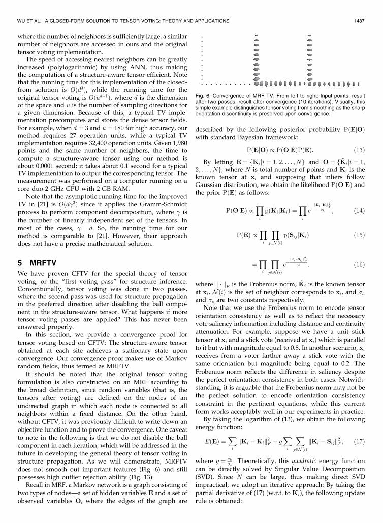
We have proven CFTV for the special theory of tensorvoting, or the “first voting pass” for structure inference.Conventionally, tensor voting was done in two passes,where the second pass was used for structure propagationin the preferred direction after disabling the ball compo-nent in the structure-aware tensor. What happens if moretensor voting passes are applied? This has never beenanswered properly.

In this section, we provide a convergence proof fortensor voting based on CFTV: The structure-aware tensorobtained at each site achieves a stationary state uponconvergence. Our convergence proof makes use of Markovrandom fields, thus termed as MRFTV.

It should be noted that the original tensor votingformulation is also constructed on an MRF according tothe broad definition, since random variables (that is, thetensors after voting) are defined on the nodes of anundirected graph in which each node is connected to allneighbors within a fixed distance. On the other hand,without CFTV, it was previously difficult to write down anobjective function and to prove the convergence. One caveatto note in the following is that we do not disable the ballcomponent in each iteration, which will be addressed in thefuture in developing the general theory of tensor voting instructure propagation. As we will demonstrate, MRFTVdoes not smooth out important features (Fig. 6) and stillpossesses high outlier rejection ability (Fig. 13).

Recall in MRF, a Markov network is a graph consisting oftwo types of nodes—a set of hidden variables E and a set ofobserved variables O, where the edges of the graph are

described by the following posterior probability PðEjOÞwith standard Bayesian framework:

PðEjOÞ / PðOjEÞPðEÞ: ð13Þ

By letting E ¼ fKiji ¼ 1; 2; . . . ; Ng and O ¼ f ~Kiji ¼ 1;2; . . . ; Ng, where N is total number of points and ~Ki is theknown tensor at xi and supposing that inliers followGaussian distribution, we obtain the likelihood PðOjEÞ andthe prior PðEÞ as follows:

PðOjEÞ /Yi

pð ~KijKiÞ ¼Yi

e�kKi� ~Kik2F

�h ; ð14Þ

PðEÞ /Yi

Yj2NðiÞ

pðSijjKiÞ ð15Þ

¼Yi

Yj2NðiÞ

e�kKi�Sijk2F

�s ; ð16Þ

where k � kF is the Frobenius norm, ~Ki is the known tensorat xi, NðiÞ is the set of neighbor corresponds to xi, and �hand �s are two constants respectively.

Note that we use the Frobenius norm to encode tensororientation consistency as well as to reflect the necessaryvote saliency information including distance and continuityattenuation. For example, suppose we have a unit sticktensor at xi and a stick vote (received at xi) which is parallelto it but with magnitude equal to 0.8. In another scenario, xireceives from a voter farther away a stick vote with thesame orientation but magnitude being equal to 0.2. TheFrobenius norm reflects the difference in saliency despitethe perfect orientation consistency in both cases. Notwith-standing, it is arguable that the Frobenius norm may not bethe perfect solution to encode orientation consistencyconstraint in the pertinent equations, while this currentform works acceptably well in our experiments in practice.

By taking the logarithm of (13), we obtain the followingenergy function:

EðEÞ ¼Xi

kKi � ~Kik2F þ g

Xi

Xj2NðiÞ

kKi � Sijk2F ; ð17Þ

where g ¼ �h�s

. Theoretically, this quadratic energy functioncan be directly solved by Singular Value Decomposition(SVD). Since N can be large, thus making direct SVDimpractical, we adopt an iterative approach: By taking thepartial derivative of (17) (w.r.t. to Ki), the following updaterule is obtained:


Fig. 6. Convergence of MRF-TV. From left to right: Input points, resultafter two passes, result after convergence (10 iterations). Visually, thissimple example distinguishes tensor voting from smoothing as the sharporientation discontinuity is preserved upon convergence.

K�i ¼ ~Ki þ 2gXj2NðiÞ

Sij

0@

1A Iþ g

Xj2NðiÞ

�Iþ c2

ijR0ij

2�0@

1A�1

;

ð18Þ

which is a Gauss-Seidel solution. When successive over-

relaxation (SOR) is employed, the update rule becomes

Kðmþ1Þi ¼ ð1� qÞKðmÞi þ qK�i ; ð19Þ

where 1 < q < 2 is the SOR weight and m is the iteration

number. After each iteration, we normalize Ki such that the

eigenvalues of the corresponding eigensystem are within

the range ð0; 1�.The above proof on convergence of MRF-TV shows that

structure-aware tensors achieve stationary states after a

finite number Gauss-Seidel iterations in the above formula-

tion. It also dispels a common pitfall that tensor voting is

similar in effect to smoothing. Using the same scale of

analysis (that is, in (2)) and the same �h, �s in each iteration,

tensor saliency and orientation will both converge. We

observe that the converged tensor orientation is, in fact,

similar to that obtained after two voting passes using the

original framework, where the orientations at curve junc-

tions are not smoothed out. See Fig. 6 for an example where

sharp orientation discontinuity is not smoothed out when

tensor voting converges. Here, 1 of each structure-aware

tensor is not normalized to 1 for visualizing its structure

saliency after convergence. Table 1 summarizes the quanti-

tative comparison with the ground-truth orientation.

6 EMTV

Previously, while tensor voting was capable of rejecting

outliers, it fell short of producing accurate parameter

estimation, explaining the use of RANSAC in the final

parameter estimation step after outlier rejection [27].This section describes the EMTV algorithm for optimiz-

ing 1) the structure-aware tensor K at each input site, and

2) the parameters of a single plane h of any dimensionality

containing the inliers. This algorithm will be applied to

stereo matching.We first formulate the three constraints to be used in

EMTV. These constraints are not mutually exclusive, where

knowing the values satisfying one constraint will help

computing the values of the others. However, in our case,

they are all unknowns, so EM is particularly suitable for

their optimization since the expectation calculation and

parameter estimation are solved alternately.

6.1 Constraints

Data constraint. Suppose we have a set of clean data. Onenecessary objective is to minimize the following for all xi 2IRd with d > 1: xTi h

; ð20Þ

where h 2 IRd is a unit vector representing the plane (orthe model) to be estimated.5 This is a typical data termthat measures the faithfulness of the input data to thefitting plane.

Orientation consistency. The plane being estimated isdefined by the vector h. Since the tensor Ki 2 IRd � IRd

encodes structure awareness, if xi is an inlier, the orienta-tion information encoded by Ki and h has to be consistent.That is, the variance hTK�1

i h produced by h should beminimal. Otherwise, xi might be generated by other modelseven if it minimizes (20). Mathematically, we minimizehTK�1

i h: ð21Þ

Neighborhood consistency. While the estimated Ki

helps to indicate inlier/outlier information, Ki has to beconsistent with the local structure imposed by its neighbors(when they are known). If Ki is consistent with h but notthe local neighborhood, either h or Ki is wrong. In practice,we minimize the following Frobenius norm as in (14)-(16):K�1

i � S0ijF: ð22Þ

In the spirit of MRF, S0ij encodes the tensor informationwithin xi’s neighborhood, thus a natural choice for definingthe term for measuring neighborhood orientation consis-tency. This is also useful, as we will see, to the M-step ofEMTV which makes the MRF assumption.

The above three constraints will interact with each otherin the proposed EM algorithm.

6.2 Objective Function

Define O ¼ foi ¼ xiji ¼ 1; . . . ; Ng to be the set of observa-tions. Our goal is to optimize h and K�1

i given O.Mathematically, we solve the objective function:

�� ¼ arg max�

P ðO;Rj�Þ; ð23Þ

where P ðO;Rj�Þ is the complete-data likelihood to bemaximized, R ¼ frig is a set of hidden states indicating ifobservation oi is an outlier (ri ¼ 0) or inlier (ri ¼ 1), and� ¼ ffK�1

i g;h; �; �; �1; �2g is a set of parameters to beestimated. �, �, �1, and �2 are parameters imposed by somedistributions, which will be explained shortly by using anequation to be introduced.6 Our EM algorithm estimates anoptimal �� by finding the value of the complete-data loglikelihood with respect to R given O and the currentestimated parameters �0:

Qð�;�0Þ ¼XR2

logP ðO;Rj�ÞP ðRjO;�0Þ; ð24Þ


TABLE 1Comparison with Ground Truth for the Example in Fig. 6

5. Note that, in some cases, the underlying model is represented in thisform xTi h� zi, where we can rearrange it into the form given by (20). Forexample, expand xTi h� zi into axi þ byi þ 1zi ¼ 0, which can written in theform of (20).

6. See the M-step in (30).

where is a space containing all possible configurations ofR of size N . Although EM does not guarantee a globaloptimal solution theoretically, because CFTV provides goodinitialization we will demonstrate empirically that reason-able results can be obtained.

6.3 Expectation (E-Step)

In this section, the marginal distribution pðrijoi;�0Þ will bedefined so that we can maximize the parameters in the nextstep (M-Step) given the current parameters.

If ri ¼ 1, the observation oi is an inlier and thereforeminimizes the first two conditions ((20) and (21)) inSection 6.1, that is, the data and orientation constraints.In both cases, we assume that inliers follow a Gaussiandistribution which explains the use of K�1

i instead of Ki.7

We model pðoijri;�0Þ as

/exp �kx

Ti hk2

2�2

� �exp �kh

TK�1i hk

2�21

� �; if ri ¼ 1;

1

C; if ri ¼ 0:

8><>: ð25Þ

We assume that outliers follow uniform distribution,where C is a constant that models the distribution. Let Cmbe the maximum dimension of the bounding box of theinput. In practice, Cm � C � 2Cm produces similar results.

Since we have no prior information on a point being aninlier or outlier, we may assume that the mixture prob-ability of the observations pðri ¼ 1Þ ¼ pðri ¼ 0Þ equals aconstant � ¼ 0:5 such that we have no bias to eithercategory (inlier/outlier). For generality in the following,we will include � in the derivation.

Define wi ¼ pðrijoi;�0Þ to be the probability of oi being aninlier. Then,

wi ¼ pðri ¼ 1joi;�0Þ ¼pðoi; ri ¼ 1j�0Þ

pðoij�0Þ

¼� exp � kx

Ti hk2

2�2

� �exp �kh

TK�1i hk

2�21

� �� exp �kx

Ti hk2

2�2

� �exp �kh

TK�1i hk

2�21

� �þ 1��

C

;

ð26Þ

where ¼ 12��1�

is the normalization term.

6.4 Maximization (M-Step)

In the M-Step, we maximize (24) using wi obtained from theE-Step. Since neighborhood information is considered, wemodel P ðO;Rj�Þ as an MRF:

P ðO;Rj�Þ ¼Yi

Yj2GðiÞ

pðrijrj;�Þpðoijri;�Þ; ð27Þ

where GðiÞ is the set of neighbors of i. In theory, GðiÞcontains all the input points except i since cij in (2) is alwaysnonzero (because of the long tail of the Gaussian distribu-tion). In practice, we can prune away the points in GðiÞwhere the values of cij are negligible. This can greatlyreduce the size of the neighborhood. Again, using ANN tree[1], the speed of searching for nearest neighbors can begreatly increased.

Let us examine the two terms in (27). pðoijri;�Þ has beendefined in (25). We define pðrijrj;�Þ here. Using the thirdcondition mentioned in (22), we have

pðrijrj;�Þ ¼ exp �K�1

i � S0ij2

F

2�22

!: ð28Þ

We are now ready to expand (24). Since ri can only assumetwo values (0 or 1), we can rewrite Qð�;�0Þ in (24) into thefollowing form:

Xt2f0;1g

logYi

Yj2GðiÞ

pðri ¼ tjrj;�Þpðoijri ¼ t;�Þ

0@

1AP ðRjO;�0Þ:

After expansion,

Qð�;�0Þ ¼Xi

log �1

�ffiffiffiffiffiffi2�p exp �kx

Ti hk2

2�2

! !wi

þXi

log1

�1

ffiffiffiffiffiffi2�p exp �kh

TK�1i hk

2�21

� �� wi

þXi

log exp �kK�1

i � S0ijk2F

2�22

! !wiwj

þXi

log1� �C

� �ð1� wiÞ:

ð29Þ

To maximize (29), we set the first derivative of Q withrespect to K�1

i , h, �, �, �1, and �2 to zero, respectively, toobtain the following set of update rules:

� ¼ 1

N

Xi

wi;

K�1i ¼

1Pj2GðiÞ wj

Xj2GðiÞ

S0ijwj ��2

2

2�21

hhTwi

0@

1A;

minkMhk subject to khk ¼ 1

�2 ¼P

i

xTi h2wiP

i wi;

�21 ¼

Pi

hTK�1i h

wiPi wi

;

�22 ¼

Pi

Pj2GðiÞ

K�1i � S0ij

2

FwiwjP

i wi;

ð30Þ

where M ¼P

i xixTi wi þ �2

�21

Pi K�1i wi and GðiÞ is a set of

neighbors of i. Equation (30) constitutes the set of update

rules for the M-step.In each iteration, after the update rules have been

executed, we normalize K�1i onto the feasible solution space

by normalization, that is, the eigenvalues of the correspond-ing eigensystem are within the range ð0; 1�. Also, S0ij will beupdated with the newly estimated K�1

i .

6.5 Implementation and Initialization

In summary, (12), (26), and (30) are all the equations neededto implement EMTV and therefore the implementation isstraightforward.

Noting that initialization is important to an EM algo-rithm, to initialize EMTV we set �1 to be a very large value,


7. Although a linear structure is being optimized here, the inlierstogether may describe a structure that does not necessarily follow anyparticular model. Each inlier may not exactly lie on this structure where themisalignment follows the Gaussian distribution.

Ki ¼ I and wi ¼ 1 for all i. S0ij is initialized to be the inverse

of Sij, computed using the closed-form solution presented

in the previous section. These initialization values mean

that at the beginning we have no preference for the surface

orientation. So, all the input points are initially considered

as inliers. With such initialization, we execute the first and

the second rules in (30) in sequence. Note that when the first

rule is being executed, the term involving h is ignored

because of the large �1; thus we can obtain K�1i for the

second rule. After that, we can start executing the algorithm

from the E-step. This initialization procedure is used in all

the experiments in the following sections. Fig. 7 shows the

result after the first EMTV iteration on an example; note in

particular that even though the initialization is at times not

close to the solution, our EMTV algorithm can still converge

to the desired ground-truth solution.

7 EXPERIMENTAL RESULTS

First, quantitative comparison will be studied to evaluate

EMTV with well-known algorithms: RANSAC [7], ASSC

[28], and TV [19]. In addition, we also provide the result

using the least squares method as a baseline comparison.

Second, we apply our method to real data with synthetic

outliers and/or noise where the ground truth is available,

and perform comparison. Third, more experiments on

multiview stereo matching on real images are performed.As we will show, EMTV performed the best in highly

corrupted data because it is designed to seek one linear

structure of known type (as opposed to multiple, potentially

nonlinear structures of unknown type). The use of orienta-

tion constraints, in addition to position constraints, makes

EMTV superior to the random sampling methods as well.Outlier/inlier (OI) ratio. We will use the outlier/inlier

ratio to characterize the outlier level, which is related to the

outlier percentage Z 2 ½0; 1�:

Z ¼ R

Rþ 1; ð31Þ

where R is the OI ratio. Fig. 7 shows a plot of Z ¼ RRþ1 ,

indicating that it is much more difficult for a given methodto handle the same percentage increase in outliers as thevalue of Z increases. Note the rapid increase in the numberof outliers as Z increases from 50 to 99 percent. That is, it ismore difficult for a given method to tolerate an addition of,say, 20 percent outliers when Z is increased from 70 to90 percent than from 50 to 70 percent. Thus, the OI ratiogives more insight in studying an algorithm’s performanceon severely corrupted data.

7.1 Robustness

We generate a set of 2D synthetic data to evaluate theperformance on line fitting, by randomly sampling 44 pointsfrom a line within the range ½�1;�1� � ½1; 1� where thelocations of the points are contaminated by Gaussian noiseof 0.1 standard deviation. Random outliers were added tothe data with different OI ratios.

The data set is then partitioned into two:

. SET 1: OI ratio 2 ½0:1; 1� with step size 0.1,

. SET 2: OI ratio 2 ½1; 100� with step size 1.

In other words, the partition is done at 50 percent outliers.Note from the plot in Fig. 7 that the number of outliersincreases rapidly after 50 percent outliers. Sample data setswith different OI ratios are shown at the top of Fig. 7.Outliers were added within a bounding circle of radius 2. Inparticular, the bottom of Fig. 7 shows the result of the firstEMTV iteration upon initialization using CFTV.

The input scale which is used in RANSAC, TV andEMTV was estimated automatically by TSSE proposed in[28]. Note, in principle these scales are not the same becauseTSSE estimates the scales of residuals in the normal space.Therefore, the scales estimated by TSSE used in TV andEMTV are only approximations. As we will demonstrate


Fig. 7. The top-left subfigure shows the plot of RRþ1 . The four 2D data sets shown here have OI ratios ½1; 20; 45; 80�, respectively, which correspond to

outlier percentages [50, 95, 98, 99 percent]. Our EMTV can tolerate OI ratios � 51 in this example. The original input, the estimated line after the firstEMTV iteration using CFTV to initialize the algorithm, and the line parameters after the first EMTV iteration and final EMTV convergence wereshown. The ground-truth parameter is ½�0:71; 0:71�.

below, even with such rough approximations, EMTV stillperforms very well, showing that it is not sensitive to scaleinaccuracy, a nice property of tensor voting which will beshown in an experiment to be detailed shortly. Note thatASSC [28] does not require any input scale.

SET 1—Refer to the left of Fig. 8, which shows the errorproduced by various methods tested on SET 1. The error ismeasured by the angle between the estimated line and theground truth. Except for the least squares method, weobserve that all the tested methods (RANSAC, ASSC, TV,and EMTV) performed very well with OI ratios � 1. ForRANSAC and ASSC, all the detected inliers were finallyused in parameter estimation. Note that the errorsmeasured for RANSAC and ASSC were the average errorsin 100 executions.8 Fig. 8 also shows the maximum andminimum errors of the two methods after running 100trials. EMTV does not have such maximum and minimumerror plots because it is deterministic.

Observe that the errors produced by our method arealmost zero in SET 1. EMTV is deterministic and convergesquickly, capable of correcting Gaussian noise inherent inthe inliers and rejecting spurious outliers, and resulting inthe almost-zero error curve. RANSAC and ASSC have error< 0:6 degree , which is still very acceptable.

SET 2—Refer to the right of Fig. 8, which shows the resultfor SET 2, from which we can distinguish the performance ofthe methods. TV breaks down at OI ratios � 20. After that,the performance of TV is unpredictable. EMTV breaks downat OI ratios � 51, showing greater robustness than TV in thisexperiment due to the EM parameter fitting procedure.

The performances of RANSAC and ASSC were quitestable where the average errors are within 4 and 7 degreesover the whole spectrum of OI ratios considered. Themaximum and minimum errors are shown in the bottom of

Fig. 8, which shows that they can be very large at times.

EMTV produces almost zero errors with OI ratio � 51, but

then breaks down with unpredictable performance. From

the experiments on SET 1 and SET 2 we conclude that EMTV

is robust up to an OI ratio of 51 (’ 98:1% outliers).Insensitivity to choice of scale. We studied the errors

produced by EMTV with different scales �d ((2)), given OI

ratio of 10 (’ 91% outliers). Even in the presence of many

outliers, EMTV broke down only when �d ’ 0:7 (the ground

truth �d is 0.1), which indicates that our method is not

sensitive to large deviations of scale. Note that the scale

parameter can sometimes be automatically estimated (e.g.,

by modifying the original TSSE to handle tangent space) as

was done in the previous experiment.Large measurement errors. In this experiment, we

increased the measurement error by increasing the stan-

dard deviation (s.d.) from 0.01 to 0.29, while keeping the

OI ratio equal to 10 and the location of the outliers fixed.

Some of the input data sets are depicted in Fig. 9, showing

that the inliers are less salient as the standard deviation

(s.d.) increases. A similar experiment was also performed

in [20]. Again, we compared our method with RANSAC,

ASSC, and TV.According to the error plot at the top of Fig. 10, TV is very

sensitive to the change of s.d.: When the s.d. is greater than

0.03, the performance is unpredictable. With increasing s.d.,

the performances of RANSAC and ASSC degrade grace-

fully, while ASSC always outperforms RANSAC. The

bottom of Fig. 10 shows the corresponding maximum and

minimum error in 100 executions.On the other hand, we observe the performance of EMTV

(with �d ¼ 0:05) is extremely steady and accurate when

s:d: < 0:15. After that, although its error plot exhibits some

perturbation, the errors produced are still small and the

performance is quite stable compared with other methods.


Fig. 8. Error plots for SET 1 (OI ratio ¼ ½0:1; 1�, up to 50 percent outliers) and SET 2 (OI ratio ¼ ½1; 100�, � 50% outliers). Left: For SET 1, all the testedmethods except for the least-squares demonstrated reliable results. EMTV is deterministic and converges quickly, capable of correcting Gaussiannoise inherent in the inliers and rejecting spurious outliers, and resulting in the almost-zero error curve. Right: For SET 2, EMTV still has an almost-zero error curve up to an OI ratio of 51 (’ 98:1% outliers). We ran 100 trials in RANSAC and ASSC and averaged the results. The maximum andminimum errors of RANSAC and ASSC are shown below each error plot.

8. We executed the algorithm 100 times. In each execution, iterativerandom sampling was done where the desired probability of choosing atleast one sample free from outliers was set to 0.99 (default value).

7.2 Fundamental Matrix Estimation

Given an image pair with p � 8 correspondences P ¼fðui;u0iÞj8 � i � pg, the goal is to estimate the 3� 3 funda-mental matrix F ¼ ½f�a;b, where a; b 2 f1; 2; 3g, such that

u0Ti Fui ¼ 0; ð32Þ

for all i. F is of rank 2. Letting u ¼ ðu; v; 1ÞT andu0 ¼ ðu0; v0; 1Þ, (32) can be rewritten into

UTi h ¼ 0; ð33Þ

where

U ¼ ðuu0; uv0; u; vu0; vv0v; u0; v0; 1ÞT ;v ¼ ðf11; f21; f31; f12; f22; f32; f13; f23; f33ÞT :

Noting that (33) is a simple plane equation, if we candetect and handle noise and outliers in the feature space,(33) should enable us to produce a good estimation.Finally, we apply [12] to obtain a rank-2 fundamentalmatrix. Data normalization is done similarly as in [12]before the optimization.

We evaluate the results by estimating the fundamentalmatrix of the data set Corridor, which is available atwww.robots.ox.ac.uk/~vgg/data.html. The matches of fea-ture points (Harris corners) are available. Random outlierswere added in the feature space.

Fig. 11 shows the plot of RMS error, which is computed

by summing up and averagingffiffiffiffiffiffiffiffiffiffiffiffiffiffiffiffiffiffiffiffiffiffiffiffiffiffiffi1p

Pi kUT

i hk2q

over all

pairs, where Ui is the set of clean data and h is the 9D

vector produced from the rank-2 fundamental matrices

estimated by various methods. Note that all the images

available in the Corridor data set are used, that is, all C112

pairs were tested. It can be observed that RANSAC breaks

down at an OI ratio ’ 20, or 95.23 percent outliers. ASSC is

very stable with RMS error < 0:15. TV breaks down at an OI

ratio ’ 10. EMTV has negligible RMS error before it starts to

break down at an OI ratio ’ 40. This finding echoes that of

Hartley [12] that linear solution is sufficient when outliers

are properly handled.

7.3 Matching

In the uncalibrated scenario, EMTV estimates parameteraccurately by employing CFTV, and effectively discardsepipolar geometries induced by wrong matches. Typically,a camera calibration is performed using nonlinear least-squares minimization and bundle adjustment [16] whichrequires good matches as input. In this experiment,candidate matches are generated by comparing the result-ing 128D SIFT feature vectors [17], so many matchedkeypoints are not corresponding.

The epipolar constraint is enforced in the matchingprocess using EMTV, which returns the fundamental matrixand the probability wi (see (26)) of a keypoint pair i being aninlier. In the experiment, we assume keypoint pair i is aninlier if wi > 0:8. Fig. 12 shows our running example teapot,which contains repetitive patterns across the whole object.Wrong matches can be easily produced by similar patternson different parts of the teapot. This data set contains30 images captured using a Nikon D70 camera. Automaticconfiguration was set during the image capture. Visually,the result produced using emtv_match is much denserthan the results produced with KeyMatchFull [25],linear_match, assc_match [28], and ransac_match.Note in particular that only emtv_match recovers theoverall geometry of the teapot, whereas the other methodscan only recover one side of the teapot.


Fig. 9. Inputs containing various measurement errors, with OI ratio ¼ 10 and fixed outliers location. The estimated models (depicted by the red lines)obtained using EMTV are overlayed on the inputs. Notice the line cluster becomes less salient when s:d: ¼ 0:25.

Fig. 10. Measurement error: Standard deviation varies from 0.01 to 0.29with OI ratio at 10. Fig. 11. Corridor. RMS error plot of various methods.

This example is challenging because the teapot’s shape isquite symmetric and the patchy patterns look identicaleverywhere. As was done in [25], each photo was paired,respectively, with a number of photos with camera posessatisfying certain basic criteria conducive to matching ormaking the numerical process stable (e.g., wide-baselinestereo). We can regard this pair-up process as one ofcomputing connected components. If the fundamentalmatrix between any successive images is incorrectlyestimated, the corresponding components will no longerbe connected, resulting in the situation where only one sideor part of the object can be recovered.

Since KeyMatchFull and linear_match use simpledistance measure for finding matches, the coverage of thecorresponding connected components tends to be small. Itis interesting to note that the worst result is produced byusing ransac_match. This can be attributed to threereasons: 1) The fundamental matrix is of rank 2, whichimplies that h spans a subspace � 8D rather than a 9Dhyperplane; 2) the input matches contain too many outliersfor some image pairs; 3) it is not feasible to fine-tune thescale parameter for every possible image pair and so weused a single value for all of the images. A slightimprovement could be found from ASSC. However, it stillsuffers from problems (1) and (2) and so the result is notvery good even compared with KeyMatchFull andlinear_match.

On the other hand, emtv_match utilizes the epipolargeometry constraint by computing the fundamental matrixin a data driven manner. Since the outliers are effectivelyfiltered out, the estimated fundamental matrices aresufficiently accurate to pair up all of the images into asingle connected component. Thus, the overall 3D geometrycan be recovered from all the available views.

7.4 Multiview Stereo Reconstruction

This section outlines how CFTV and EMTV are applied toimprove the match-propagate-filter pipeline in multiviewstereo. Match-propagate-filter is a competitive approach tomultiview stereo reconstruction for computing a (quasi)dense representation. Starting from a sparse set of initialmatches with high confidence, matches are propagatedusing photoconsistency to produce a (quasi) dense recon-struction of the target shape. Visibility consistency can beapplied to remove outliers. Among the existing works using

the match-propagate-filter approach, patch-based multi-

view stereo (or PMVS) proposed in [10] has produced some

of the best results to date.We observe that PMVS had not fully utilized the 3D

information inherent in the sparse and dense geometry

before, during, and after propagation, as patches do not

adequately communicate among each other. As noted in

[10], data communication should not be done by smooth-

ing, but the lack of communication will cause perturbed

surface normals and patch outliers during the propagation

stage. In [29], we proposed tensor-based multiview stereo

(TMVS) and used 3D structure-aware tensors which

communicate among each other via CFTV. We found that

such tensor communication not only improves propaga-

tion in MVS without undesirable smoothing but also

benefits the entire match-propagate-filter pipeline within a

unified framework.We captured 179 photos around a building which were

first calibrated as described in Section 7.3. All images were

taken on the ground level, not higher than the building, so

we have very few samples of the rooftop. The building

facades are curved and the windows on the building look

identical to each other. The patterns on the front and back

facade look nearly identical. These ambiguities cause

significant challenges in the matching stage especially for

wide-baseline stereo. TMVS was run to obtain the quasi-

dense reconstruction, where MRFTV was used to filter

outliers as shown in Fig. 13. Fig. 14 shows the 3D

reconstruction, which is faithful to the real building.

Readers are referred to [29] for more detail and experi-

mental evaluation of TMVS.


Fig. 12. Teapot: (a) Four images (one in enlarged view) from the input image set consisting of 30 images captured around the object in a casualmanner. (b)-(f) show two views of the sparse reconstruction generated by using KeyMatchFull (398 points), linear_match (493 points),ransac_match (37 points), assc_match (208 points), and emtv_match (2,152 points). The candidate matches returned by SIFT are extremelynoisy due to the ambiguous patchy patterns. On average, 17,404 trials were run in ransac_match. It is time consuming to run more trials on thisnoisy and large input where an image pair can have as many as 5,000 similar matches and similarly for assc_match, where additional running timeis needed to estimate the scale parameter in each iteration. On the other hand, emtv_match does not require any random sampling.

Fig. 13. Results before and after filtering of Hall 3 (images shown inFig. 14). All salient 3D structures are retained in the filtered result,including the bushes near the left facade and planters near the rightfacade in this top view of the building.

8 CONCLUSIONS

A closed-form solution is proven for the special theory oftensor voting (CFTV) for computing an exact structure-aware tensor in any dimensions. For structure propagation,we derive a quadratic energy for MRFTV, thus providing aconvergence proof for tensor voting which is impossible toprove using the original tensor voting procedure. Then, wederive EMTV for optimizing both the tensor and modelparameters for robust parameter estimation. We performedquantitative and qualitative evaluation using challengingsynthetic and real data sets. In the future, we will develop aclosed-form solution for the general theory of tensor voting,and extend EMTV to extract multiple and nonlinearstructures. We have provided C++ source code, but it isstraightforward to implement (11), (12), (26), (30), (18), and(19). We demonstrated promising results in multiviewstereo, and will apply our closed-form solution to addressimportant computer vision problems.

ACKNOWLEDGMENTS

The authors would like to thank the Associate Editor and all

of the anonymous reviewers. Special thanks to Reviewer 1

for his/her helpful and detailed comments throughout the

review cycle. S.-K. Yeung was supported by the Start-up

Research Grant: SRG ISTD 2011 016. J. Jia was supported by

the Hong Kong Research Grant Council (RGC, grant no.

412911). C.-K. Tang was supported by RGC (grant no.

619711) and the Google Faculty Award on quasi dense 3D

reconstruction.

REFERENCES

[1] S. Arya and D.M. Mount, “Approximate Nearest NeighborSearching,” Proc. ACM-SIAM Symp. Discrete Algorithms, pp. 271-280, 2003.

[2] J. Bilmes, “A Gentle Tutorial on the EM Algorithm and ItsApplication to Parameter Estimation for Gaussian Mixture andHidden Markov Models,” Technical Report ICSI-TR-97-021, ICSI,1997.

[3] H. Chen and P. Meer, “Robust Regression with Projection Basedm-Estimators,” Proc. Ninth IEEE Int’l Conf. Computer Vision, vol. 2,pp. 878-885, 2003.

[4] O. Chum and J. Matas, “Optimal Randomized Ransac,” IEEETrans. Pattern Analysis and Machine Intelligence, vol. 30, no. 8,pp. 1472-1482, Aug. 2008.

[5] D. Comaniciu and P. Meer, “Mean Shift: A Robust Approachtoward Feature Space Analysis,” IEEE Trans. Pattern Analysis andMachine Intelligence, vol. 24, no. 5, pp. 603-619, May 2002.

[6] R. Dahyot, “Statistical Hough Transform,” IEEE Trans. PatternAnalysis and Machine Intelligence, vol. 31, no. 8, pp. 1502-1509, Aug.2009.

[7] M.A. Fischler and R.C. Bolles, “Random Sample Consensus: AParadigm for Model Fitting with Applications to ImageAnalysis and Automated Cartography,” Comm. ACM, vol. 24,pp. 381-395, 1981.

[8] D. Forsyth and J. Ponce, Computer Vision: A Modern Approach.Prentice Hall, 2003.

[9] E. Franken, M. van Almsick, P. Rongen, L. Florack, and B. ter HaarRomeny, “An Efficient Method for Tensor Voting Using SteerableFilters,” Proc. Ninth European Conf. Computer Vision, vol. 4, pp. 228-240, 2006.

[10] Y. Furukawa and J. Ponce, “Accurate, Dense, and RobustMultiview Stereopsis,” IEEE Trans. Pattern Analysis and MachineIntelligence, vol. 32, no. 8, pp. 1362-1376, Aug. 2010.

[11] B. Georgescu, I. Shimshoni, and P. Meer, “Mean Shift BasedClustering in High Dimensions: A Texture Classification Exam-ple,” Proc. Ninth IEEE Int’l Conf. Computer Vision, pp. 456-463,2003.

[12] R. Hartley, “In Defense of the Eight-Point Algorithm,” IEEE Trans.Pattern Analysis and Machine Intelligence, vol. 19, no. 6, pp. 580-593,June 1997.

[13] P. Hough, “Machine Analysis of Bubble Chamber Pictures,” Proc.Int’l Conf. High Energy Accelerators and Instrumentation, 1959.

[14] P.J. Huber, Robust Statistics. John Wiley & Sons, 1981.[15] K. Lee, P. Meer, and R. Park, “Robust Adaptive Segmentation of

Range Images,” IEEE Trans. Pattern Analysis and Machine Intelli-gence, vol. 20, no. 2, pp. 200-205, Feb. 1998.

[16] M. Lourakis and A. Argyros, “The Design and Implementation ofa Generic Sparse Bundle Adjustment Software Package Based onthe Levenberg-Marquardt Algorithm,” Technical Report 340,ICSFORTH, 2004.

[17] D. Lowe, “Distinctive Image Features from Scale-Invariant Key-points,” Int’l J. Computer Vision, vol. 60, no. 2, pp. 91-110, Nov.2004.

[18] G.J. McLachlan and T. Krishnan, EM Algorithms and Extension.Elsevier, 1997.

[19] G. Medioni, M.S. Lee, and C.K. Tang, A Computational Frameworkfor Segmentation and Grouping. Elsevier, 2000.

[20] P. Meer, “Robust Techniques for Computer Vision,” EmergingTopics in Computer Vision, chapter 4, Prentice Hall, 2004.

[21] P. Mordohai and G. Medioni, “Dimensionality Estimation,Manifold Learning and Function Approximation Using TensorVoting,” J. Machine Learning Research, vol. 11, pp. 411-450, Jan.2010.

[22] P. Rousseeuw, “Least Median of Squares Regression,” J. Am.Statistics Assoc., vol. 79, pp. 871-880, 1984.

[23] P. Rousseeuw, Robust Regression and Outlier Detection. Wiley, 1987.[24] K. Sim and R. Hartley, “Removing Outliers Using the Linfty

Norm,” Proc. IEEE Conf. Computer Vision and Pattern Recognition,vol. 1, pp. 485-494, 2006.

[25] N. Snavely, S. Seitz, and R. Szeliski, “Modeling the World fromInternet Photo Collections,” Int’l J. Computer Vision, vol. 80, no. 2,pp. 189-210, Nov. 2008.

[26] R. Subarao and P. Meer, “Beyond Ransac: User IndependentRobust Regression,” Proc. Workshop 25 Years of Random SampleConsensus, June 2006.

[27] W.S. Tong, C.K. Tang, and G. Medioni, “Simultaneous Two-ViewEpipolar Geometry Estimation and Motion Segmentation by 4DTensor Voting,” IEEE Trans. Pattern Analysis and MachineIntelligence, vol. 26, no. 9, pp. 1167-1184, Sept. 2004.

[28] H. Wang and D. Suter, “Robust Adaptive-Scale Parametric ModelEstimation for Computer Vision,” IEEE Trans. Pattern Analysis andMachine Intelligence, vol. 26, no. 11, pp. 1459-1474, Nov. 2004.


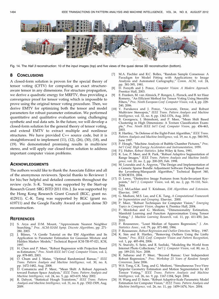
Fig. 14. The Hall 3 reconstruction: 10 of the input images (top) and five views of the quasi dense 3D reconstruction (bottom).

[29] T.P. Wu, S.K. Yeung, J. Jia, and C.K. Tang, “Quasi-Dense 3DReconstruction Using Tensor-Based Multiview Stereo,” Proc. IEEEConf. Computer Vision and Pattern Recognition, 2010.

Tai-Pang Wu received the PhD degree incomputer science from the Hong Kong Univer-sity of Science and Technology (HKUST) in2007. He was awarded the Microsoft Fellowshipin 2006. He has been employed as a post-doctoral fellow at Microsoft Research Asia andthe Chinese University of Hong Kong. He iscurrently a manager of the Enterprise andConsumer Electronics Group at the Hong KongApplied Science and Technology Research

Institute (ASTRI). He is a member of the IEEE Computer Society.

Sai-Kit Yeung received the BEng degree (FirstClass Honors) in computer engineering and theMPhil degree in bioengineering from the HongKong University of Science and Technology(HKUST) in 2003 and 2005, respectively, andthe PhD degree in electronic and computerengineering from HKUST in 2009. He was avisiting student at the Image Sciences Institute,University Medical Center Utrecht, The Nether-lands, in 2007 and the Image Processing

Research Group at the University of California Los Angeles (UCLA) in2008. He is currently an assistant professor at the Singapore Universityof Technology and Design (SUTD). Prior to joining SUTD, he was apostdoctoral scholar in the Department of Mathematics, UCLA in 2010.His research interests include computer vision, computer graphics,computational photography, image/video processing, and medicalimaging. He is a member of the IEEE Computer Society.

Jiaya Jia received the PhD degree in computerscience from the Hong Kong University ofScience and Technology in 2004 and is currentlyan associate professor in the Department ofComputer Science and Engineering at theChinese University of Hong Kong (CUHK). Hewas a visiting scholar at Microsoft ResearchAsia from March 2004 to August 2005 andconducted collaborative research at AdobeSystems in 2007. He leads the research group

at CUHK, focusing on computational photography, 3D reconstruction,practical optimization, and motion estimation. He serves as an associateeditor for the IEEE Transactions on Pattern Analysis and MachineIntelligence (TPAMI) and as an area chair for ICCV 2011. He was on theprogram committees of several major conferences, including ICCV,ECCV, and CVPR, and cochaired the Workshop on InteractiveComputer Vision in conjunction with ICCV 2007. He received the YoungResearcher Award 2008 and Research Excellence Award 2009 fromCUHK. He is a senior member of the IEEE and a member of the IEEEComputer Society.

Chi-Keung Tang received the MSc and PhDdegrees in computer science from the Universityof Southern California (USC), Los Angeles, in1999 and 2000, respectively. Since 2000, he hasbeen with the Department of Computer Scienceat the Hong Kong University of Science andTechnology (HKUST), where he is currently aprofessor. He is an adjunct researcher in theVisual Computing Group of Microsoft ResearchAsia. His research areas are computer vision,

computer graphics, and human-computer interaction. He is an associateeditor of the IEEE Transactions on Pattern Analysis and MachineIntelligence (TPAMI) and on the editorial board of the InternationalJournal of Computer Vision (IJCV). He served as an area chair forACCV 2006 (Hyderabad), ICCV 2007 (Rio de Janeiro), ICCV 2009(Kyoto), ICCV 2011 (Barcelona), and as a technical papers committeemember for the inaugural SIGGRAPH Asia 2008 (Singapore), SIG-GRAPH 2011 (Vancouver), SIGGRAPH Asia 2011 (Hong Kong), andSIGGRAPH 2012 (Los Angeles). He is a senior member of the IEEE anda member of the IEEE Computer Society.

Gerard Medioni received the Diplome d’Ingen-ieur from the �Ecole Nationale Superieure desTelecommunications (ENST), Paris, in 1977 andthe MS and PhD degrees from the University ofSouthern California (USC) in 1980 and 1983,respectively. He has been with USC since thenand is currently a professor of computer scienceand electrical engineering, a codirector of theInstitute for Robotics and Intelligent Systems(IRIS), and a codirector of the USC Games

Institute. He served as the chairman of the Computer ScienceDepartment from 2001 to 2007. He has made significant contributionsto the field of computer vision. His research covers a broad spectrum ofthe field, such as edge detection, stereo and motion analysis, shapeinference and description, and system integration. He has publishedthree books, more than 50 journal papers, and 150 conference articles.He is the holder of eight international patents. He is an associate editorof the Image and Vision Computing Journal, Pattern Recognition andImage Analysis Journal, and the International Journal of Image andVideo Processing. He served as a program cochair of the 1991 IEEEComputer Vision and Pattern Recognition (CVPR) Conference and the1995 IEEE International Symposium on Computer Vision, a generalcochair of the 1997 IEEE CVPR Conference, a conference cochair ofthe 1998 International Conference on Pattern Recognition, a generalcochair of the 2001 IEEE CVPR Conference, a general cochair of the2007 IEEE CVPR Conference, and a general cochair of the 2009 IEEECVPR Conference. He is a fellow of the IEEE, IAPR, and AAAI and amember of the IEEE Computer Society.

. For more information on this or any other computing topic,please visit our Digital Library at www.computer.org/publications/dlib.


1482 ieee transactions on pattern analysis and … · voting (cftv), which is applicable to the...

Documents