15-251 great theoretical ideas in computer …arielpro/15251f15/slides/lec20.pdfgreat theoretical...
TRANSCRIPT
15-251 Great Theoretical Ideas in Computer Science
Lecture 20:Randomized Algorithms
November 5th, 2015
So far
Formalization of computation/algorithm
Computability / Uncomputability
Computational complexity
NP-completeness. Identifying intractable problems.
Making use of intractable problems (in Social choice).
Dealing with intractable problems: Approximation algs.
Online algs.
Graph theory and graph algorithms
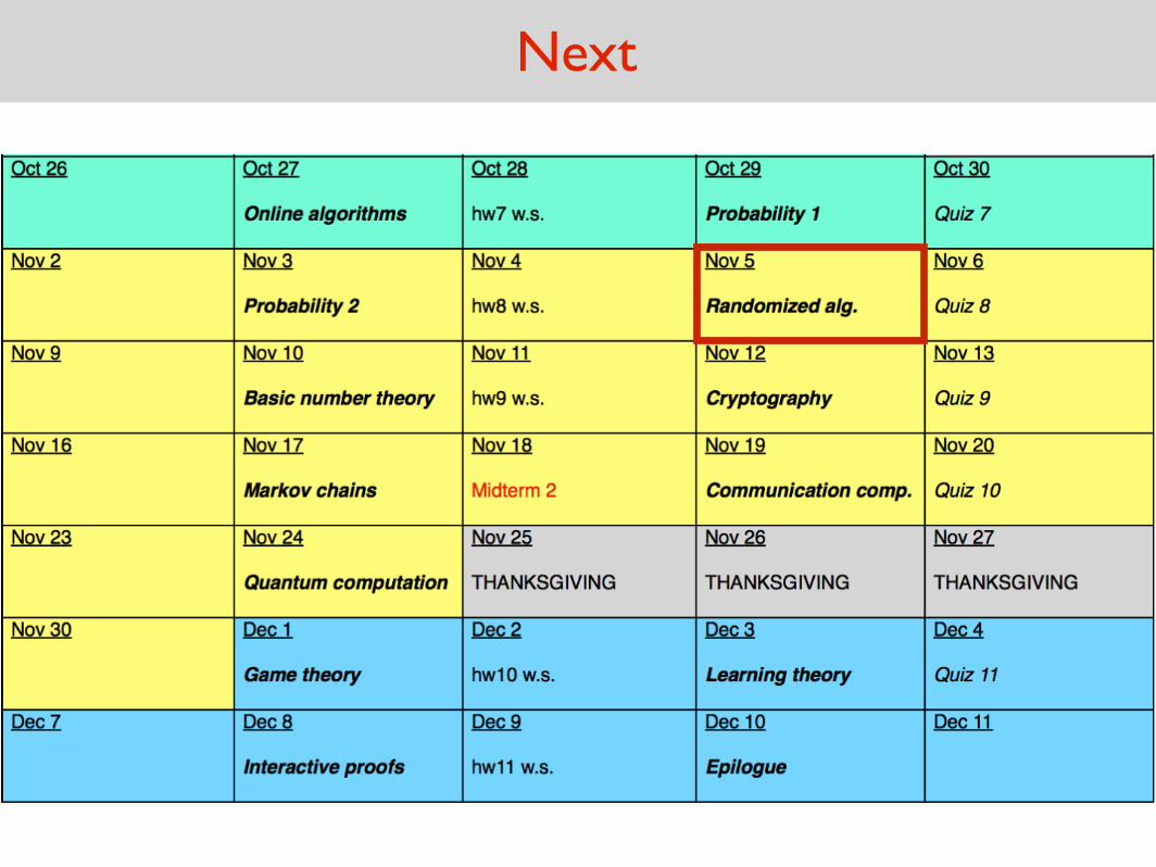
Next
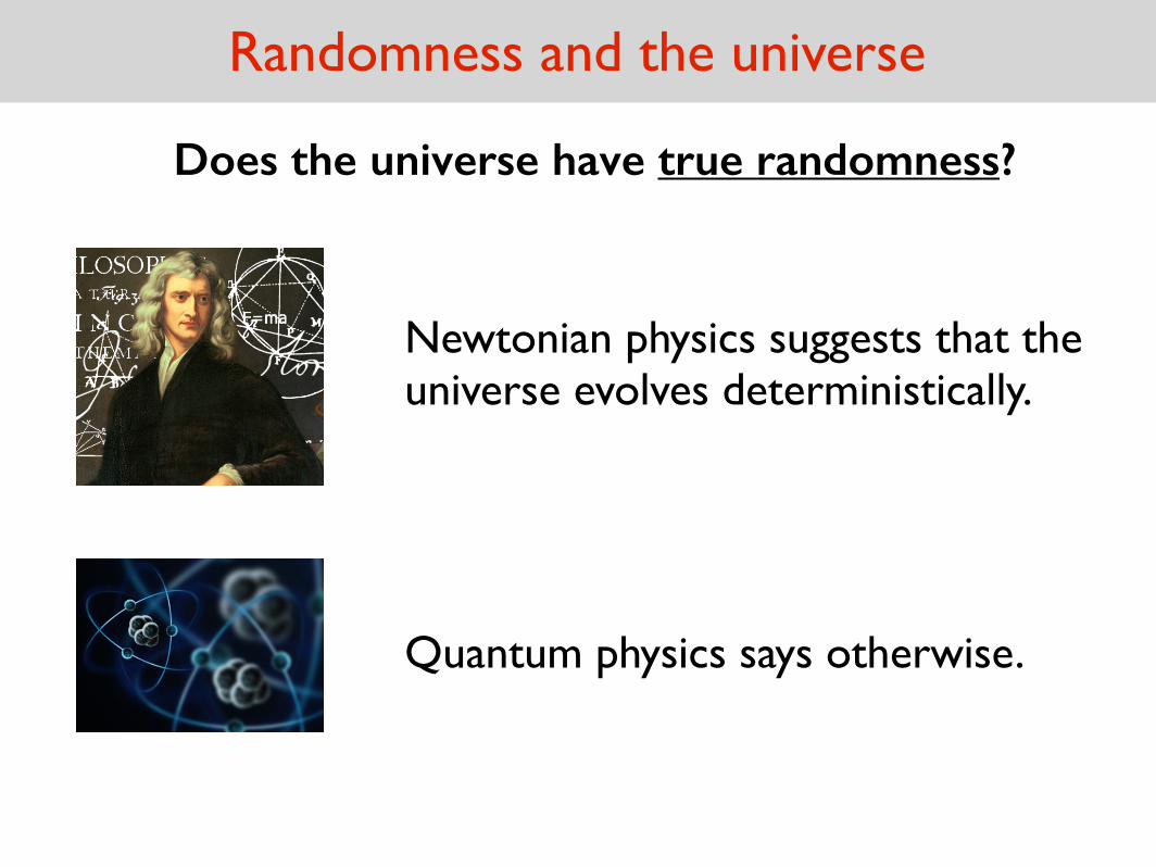
Randomness and the universe
Newtonian physics suggests that the universe evolves deterministically.
Does the universe have true randomness?
Quantum physics says otherwise.
Randomness and the universe
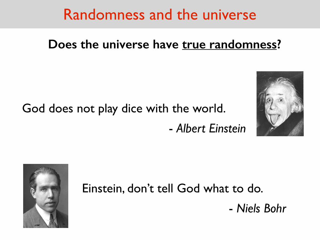
Does the universe have true randomness?
God does not play dice with the world.
- Albert Einstein
Einstein, don’t tell God what to do.
- Niels Bohr
Randomness and the universe
Does the universe have true randomness?
Even if it doesn’t, we can still model our uncertaintyabout things using probability.
Randomness is an essential tool in modeling and analyzing nature.
It also plays a key role in computer science.
Randomness in computer science
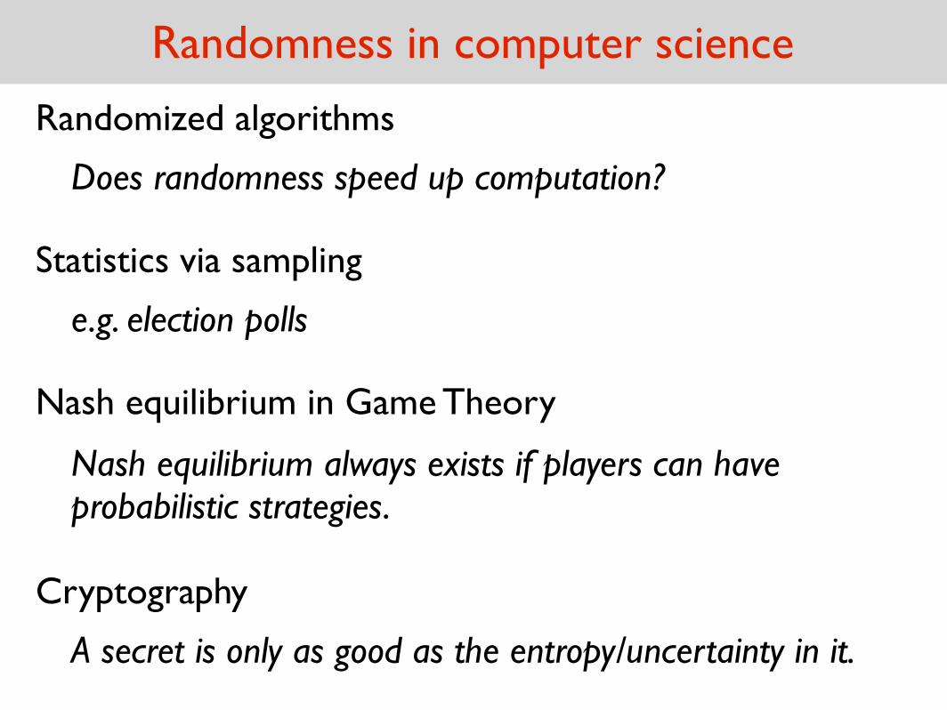
Randomized algorithms
Does randomness speed up computation?
Statistics via sampling
e.g. election polls
Nash equilibrium in Game Theory
Nash equilibrium always exists if players can have probabilistic strategies.
Cryptography
A secret is only as good as the entropy/uncertainty in it.
Randomness in computer science
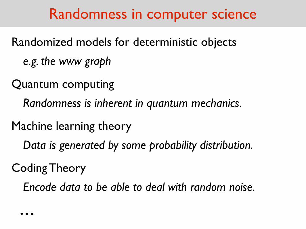
Randomized models for deterministic objects
e.g. the www graph
Quantum computing
Randomness is inherent in quantum mechanics.
…
Machine learning theory
Data is generated by some probability distribution.
Coding Theory
Encode data to be able to deal with random noise.
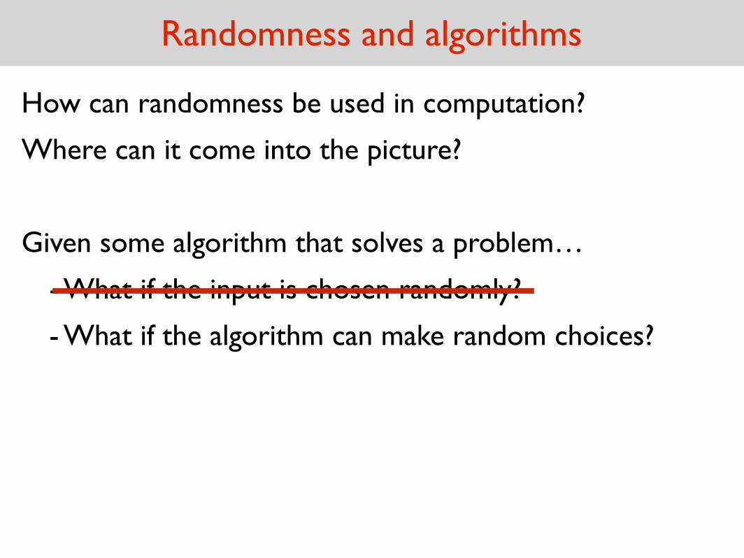
Randomness and algorithms
How can randomness be used in computation?
Where can it come into the picture?
Given some algorithm that solves a problem…
- What if the input is chosen randomly?
- What if the algorithm can make random choices?
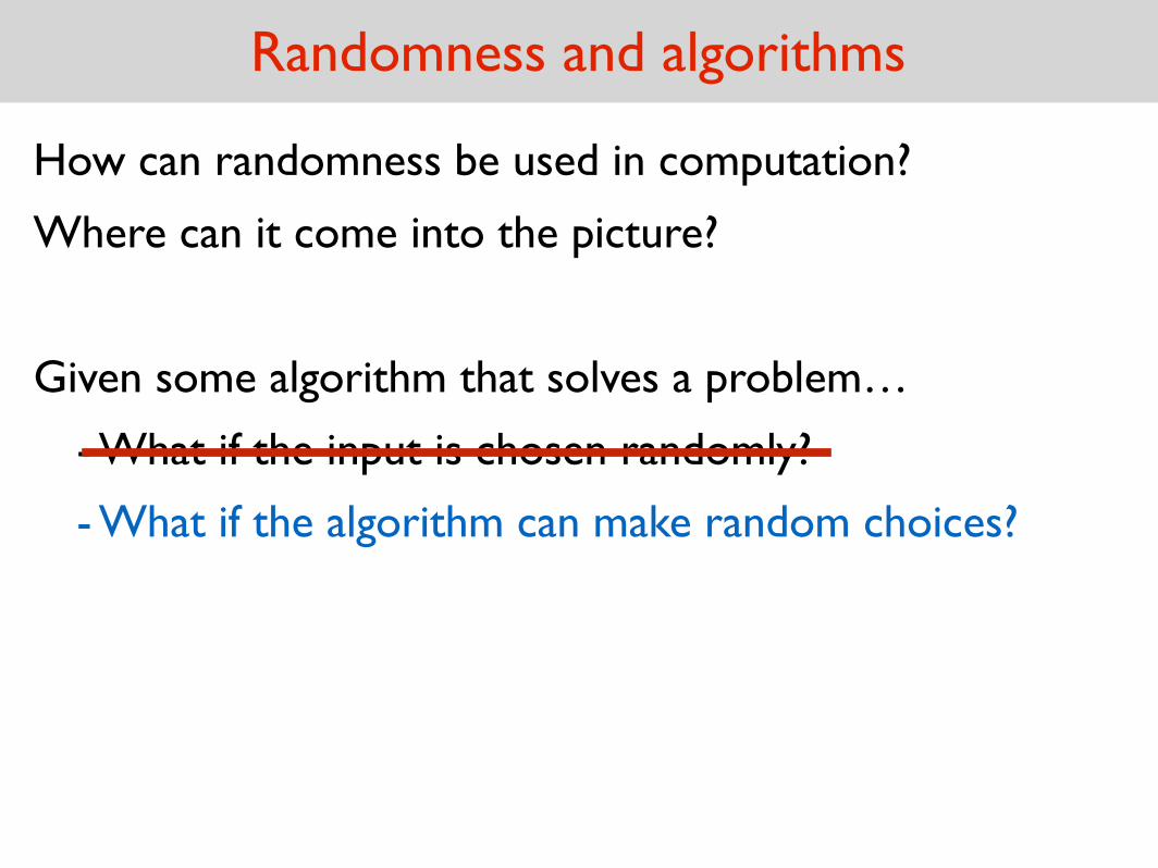
Randomness and algorithms
Given some algorithm that solves a problem…
- What if the input is chosen randomly?
- What if the algorithm can make random choices?
How can randomness be used in computation?
Where can it come into the picture?
Randomness and algorithms
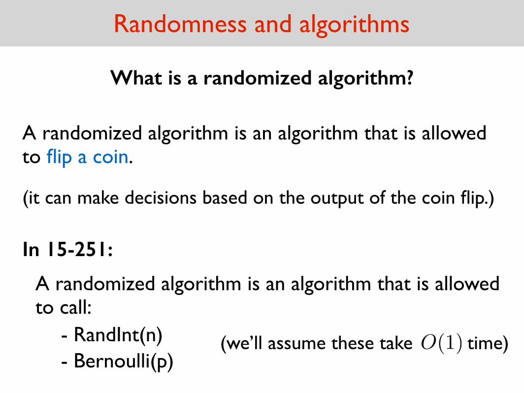
A randomized algorithm is an algorithm that is allowed to flip a coin.
What is a randomized algorithm?
(it can make decisions based on the output of the coin flip.)
In 15-251:
A randomized algorithm is an algorithm that is allowed to call:
- RandInt(n)- Bernoulli(p)
(we’ll assume these take time)O(1)
Randomness and algorithms
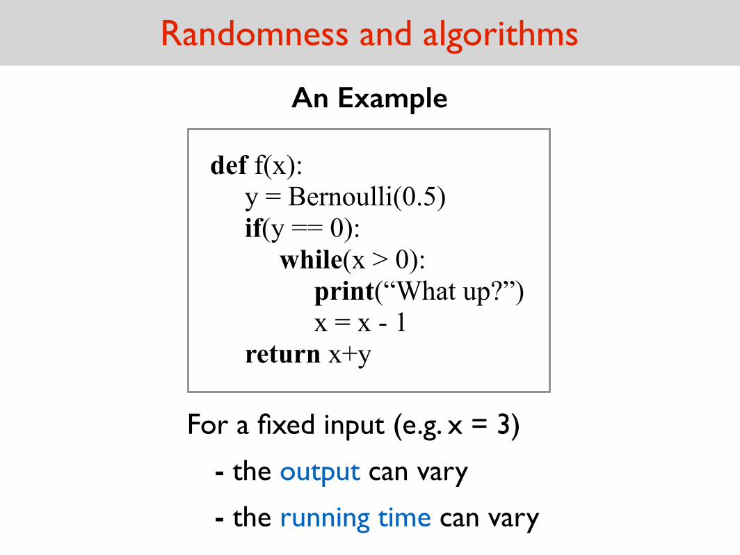
For a fixed input (e.g. x = 3)
- the output can vary
- the running time can vary
def f(x): y = Bernoulli(0.5) if(y == 0): while(x > 0): print(“What up?”) x = x - 1 return x+y
An Example
Randomness and algorithms
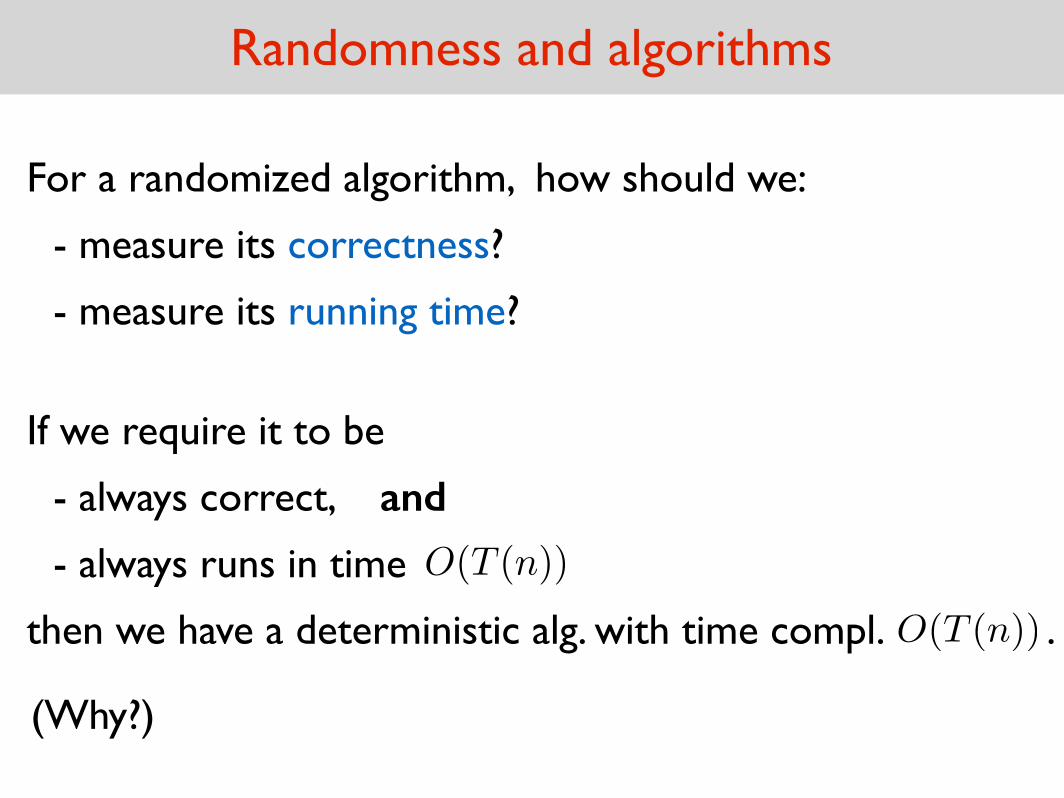
For a randomized algorithm, how should we:
- measure its correctness?
- measure its running time?
then we have a deterministic alg. with time compl. .O(T (n))
If we require it to be
- always correct, and
- always runs in time O(T (n))
(Why?)
Randomness and algorithms
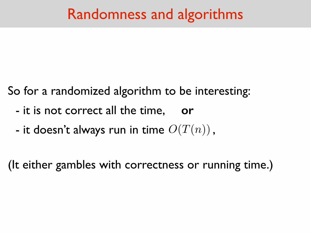
So for a randomized algorithm to be interesting:
- it is not correct all the time, or
- it doesn’t always run in time ,O(T (n))
(It either gambles with correctness or running time.)
Types of randomized algorithms
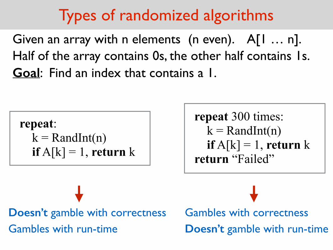
repeat: k = RandInt(n) if A[k] = 1, return k
Given an array with n elements (n even). A[1 … n].Half of the array contains 0s, the other half contains 1s.Goal: Find an index that contains a 1.
repeat 300 times: k = RandInt(n) if A[k] = 1, return k return “Failed”
Doesn’t gamble with correctnessGambles with run-time
Gambles with correctnessDoesn’t gamble with run-time
Types of randomized algorithms
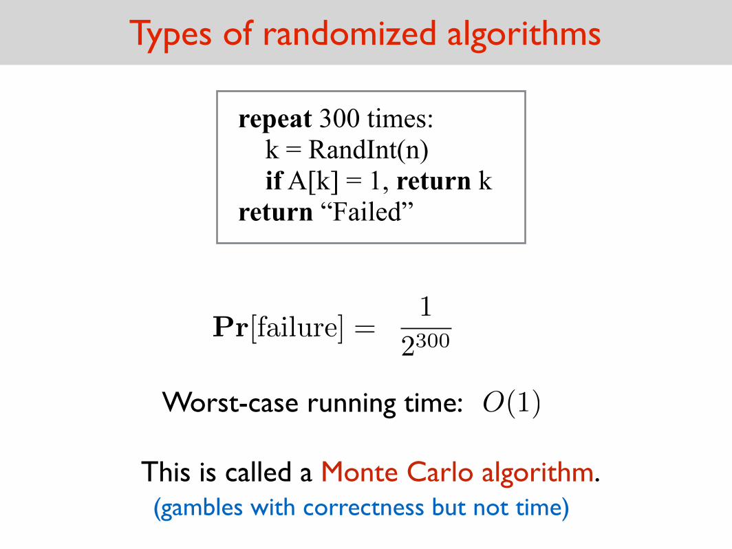
Pr[failure] =1
2300
Worst-case running time: O(1)
This is called a Monte Carlo algorithm.(gambles with correctness but not time)
repeat 300 times: k = RandInt(n) if A[k] = 1, return k return “Failed”
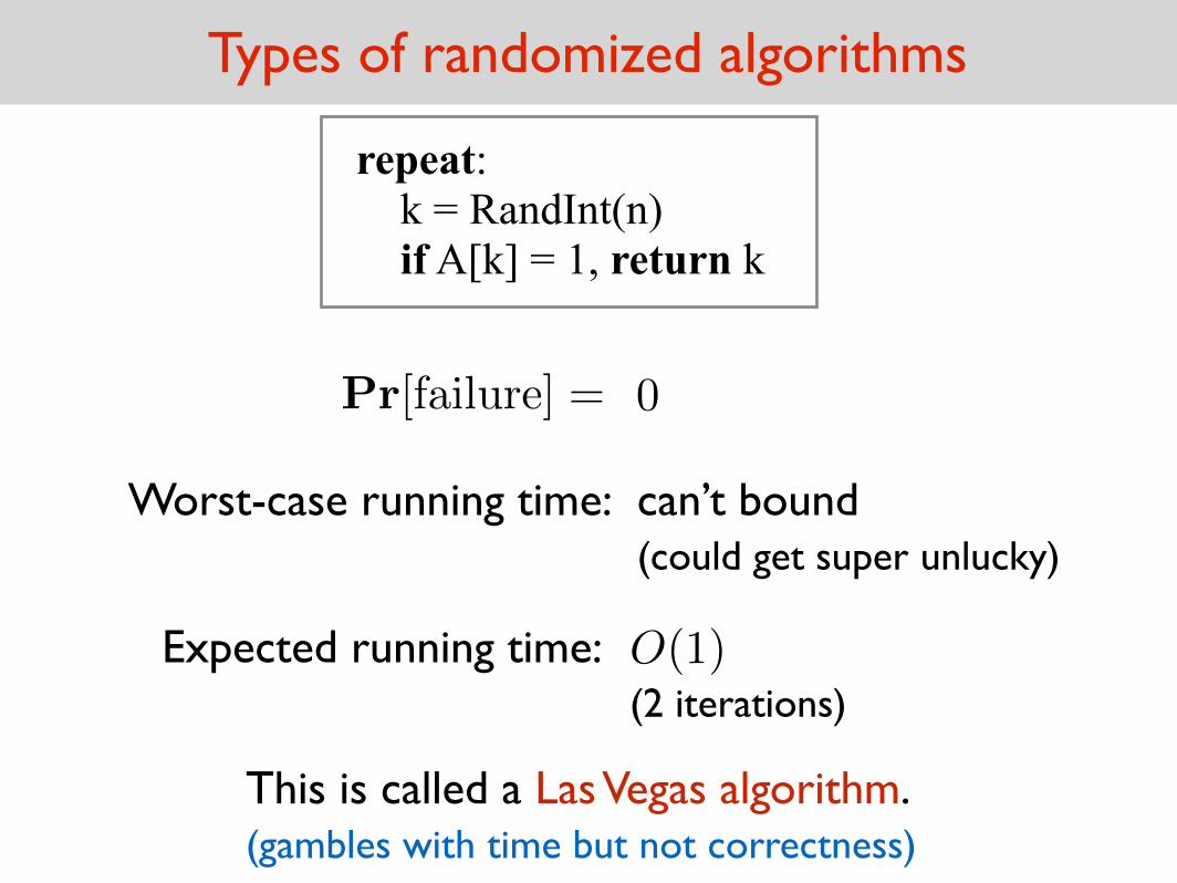
Types of randomized algorithms
Pr[failure] =
This is called a Las Vegas algorithm.
repeat: k = RandInt(n) if A[k] = 1, return k
0
can’t bound(could get super unlucky)
Worst-case running time:
Expected running time: O(1)(2 iterations)
(gambles with time but not correctness)
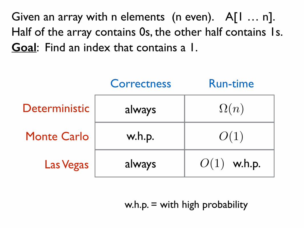
Given an array with n elements (n even). A[1 … n].Half of the array contains 0s, the other half contains 1s.Goal: Find an index that contains a 1.
Deterministic
Monte Carlo
Las Vegas
Correctness Run-time
always
always
w.h.p.
w.h.p. = with high probability
⌦(n)
O(1)
O(1) w.h.p.
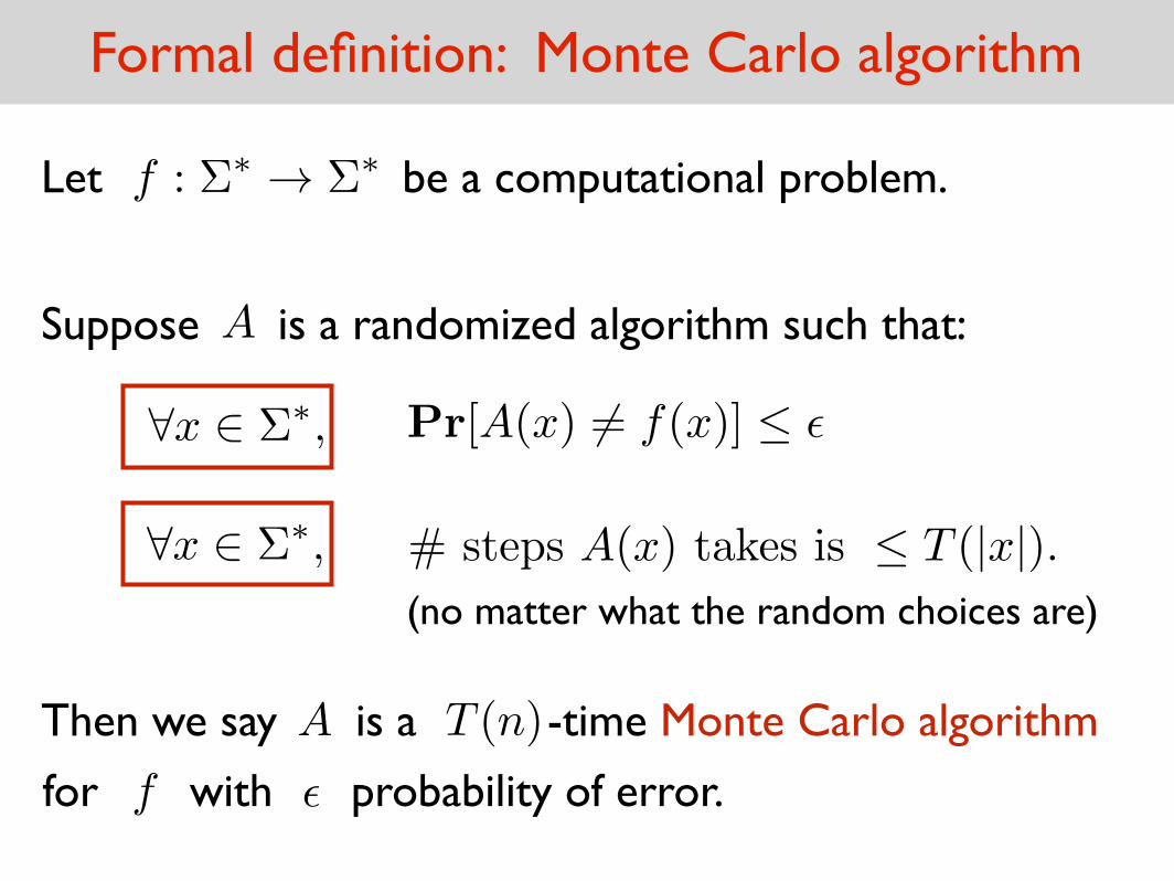
Formal definition: Monte Carlo algorithm
Let be a computational problem. f : ⌃⇤ ! ⌃⇤
Suppose is a randomized algorithm such that:A
8x 2 ⌃⇤,
Pr[A(x) 6= f(x)] ✏
8x 2 ⌃⇤, # steps A(x) takes is T (|x|).
Then we say is a -time Monte Carlo algorithm
for with probability of error.
A T (n)
f ✏
(no matter what the random choices are)
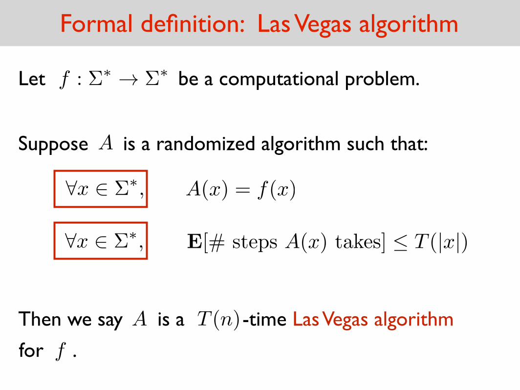
Formal definition: Las Vegas algorithm
Let be a computational problem. f : ⌃⇤ ! ⌃⇤
Suppose is a randomized algorithm such that:A
Then we say is a -time Las Vegas algorithm
for .
A T (n)
f
8x 2 ⌃⇤,
A(x) = f(x)
8x 2 ⌃⇤, E[# steps A(x) takes] T (|x|)

Example of a Monte Carlo Algorithm: Min Cut
Example of a Las Vegas Algorithm: Quicksort
NEXT ON THE MENU
Example of a Monte Carlo Algorithm: Min Cut
Gambles with correctness. Doesn’t gamble with running time.
Cut Problems
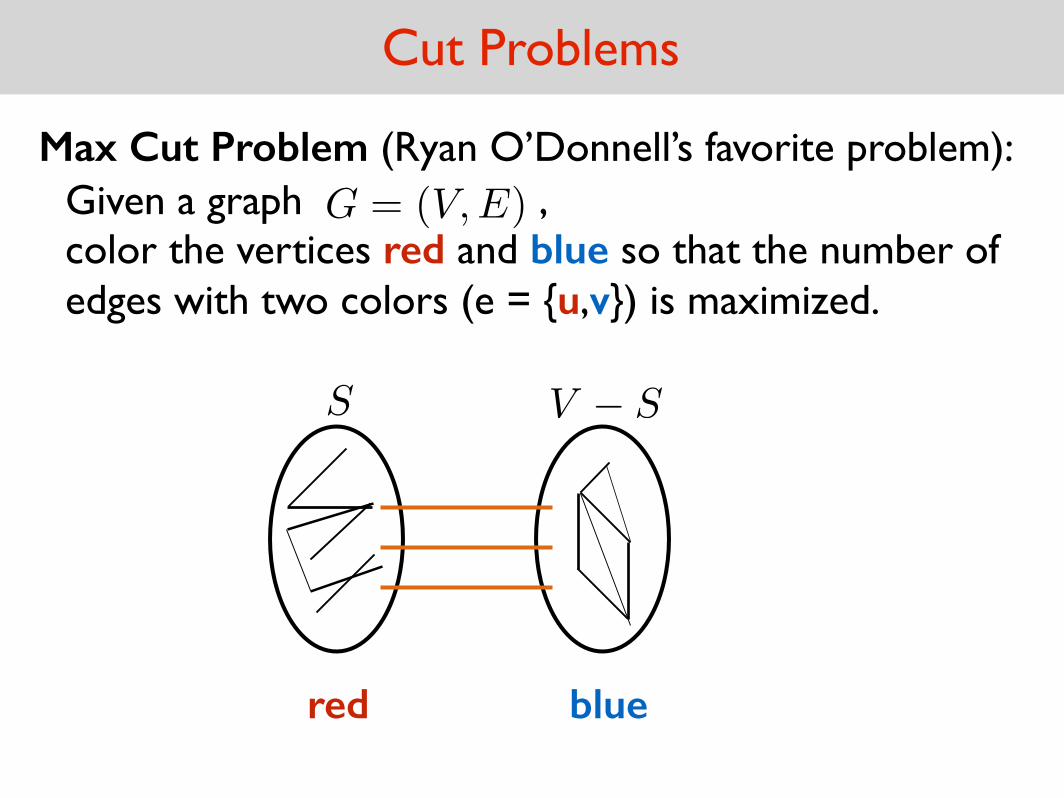
Max Cut Problem (Ryan O’Donnell’s favorite problem):Given a graph , color the vertices red and blue so that the number ofedges with two colors (e = {u,v}) is maximized.
G = (V,E)
S V � S
red blue
Cut Problems
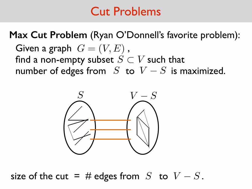
Max Cut Problem (Ryan O’Donnell’s favorite problem):Given a graph , find a non-empty subset such thatnumber of edges from to is maximized.
G = (V,E)S ⇢ VS V � S
S V � S
size of the cut = # edges from to .S V � S
Cut Problems
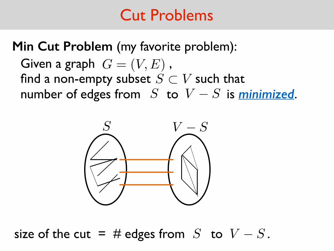
Min Cut Problem (my favorite problem):Given a graph , find a non-empty subset such thatnumber of edges from to is minimized.
G = (V,E)S ⇢ VS V � S
S V � S
size of the cut = # edges from to .S V � S
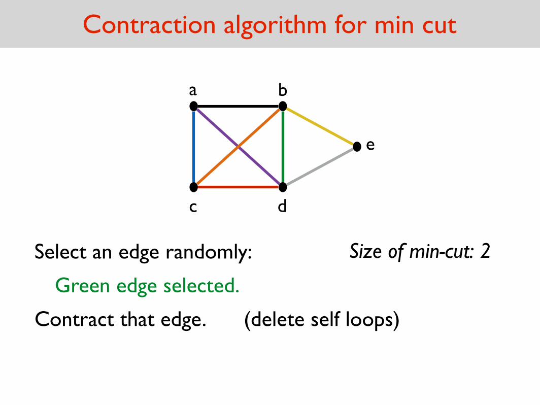
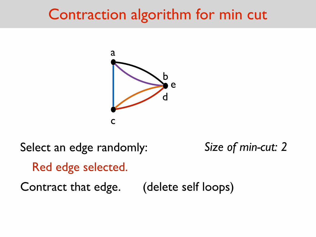
Contraction algorithm for min cut
Let’s see a super simple randomized algorithm Min-Cut.
Contraction algorithm for min cut
a
c
b
e
d
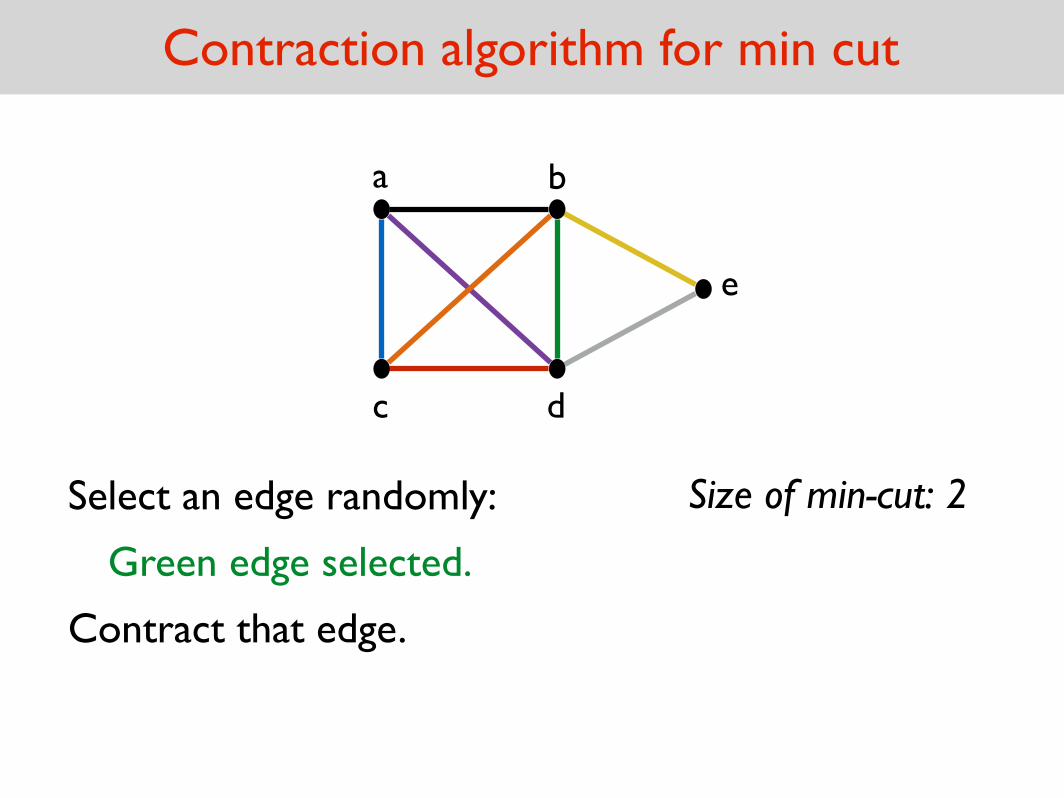
Select an edge randomly:
Green edge selected.
Contract that edge.
Size of min-cut: 2
a
c
be
d
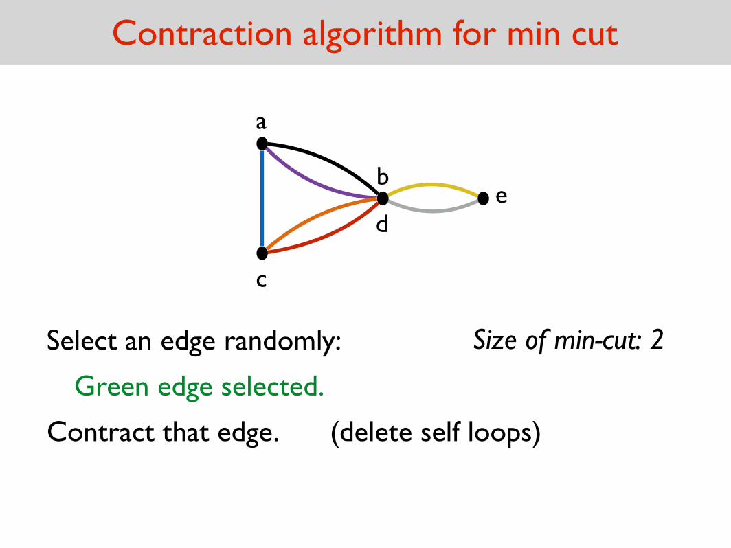
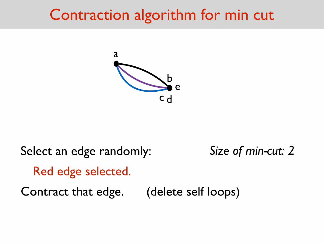
Contraction algorithm for min cut
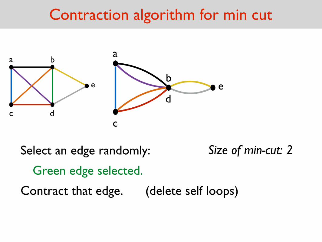
Select an edge randomly:
Green edge selected.
Contract that edge. (delete self loops)
Size of min-cut: 2
a
c
be
d
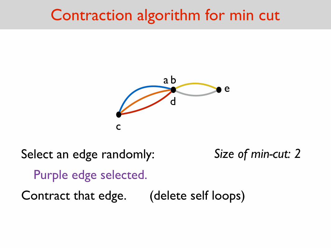
Contraction algorithm for min cut
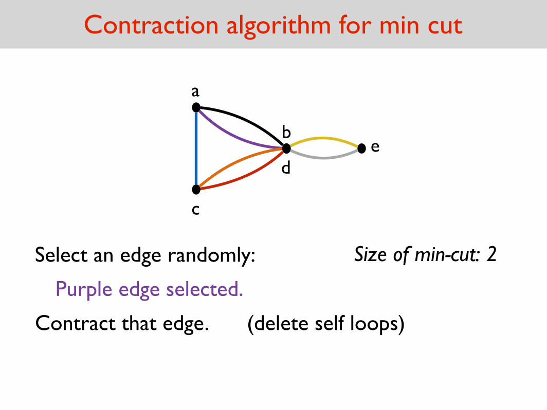
Purple edge selected.
Contract that edge. (delete self loops)
Size of min-cut: 2Select an edge randomly:
a
c
be
d
Contraction algorithm for min cut
Purple edge selected.
Contract that edge. (delete self loops)
Size of min-cut: 2Select an edge randomly:
a
c
be
d
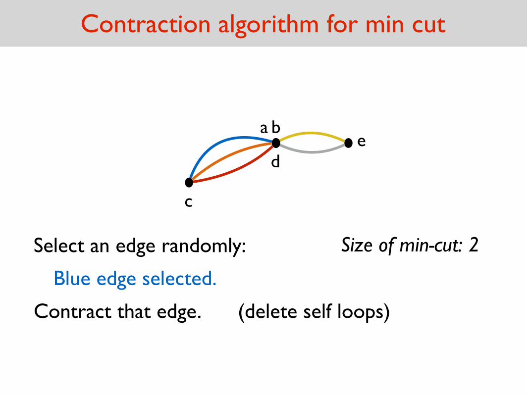
Contraction algorithm for min cut
Blue edge selected.
Contract that edge. (delete self loops)
Size of min-cut: 2Select an edge randomly:
a
c
be
d
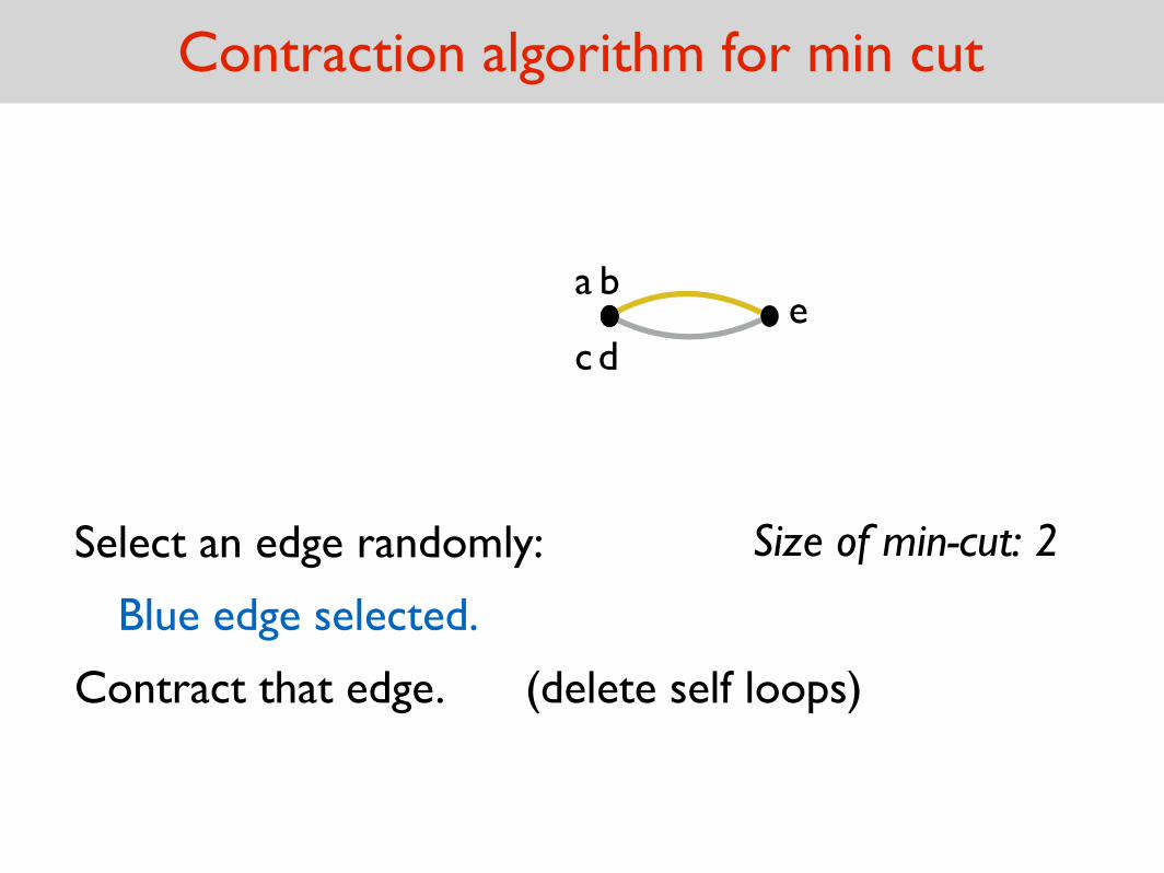
Contraction algorithm for min cut
Blue edge selected.
Contract that edge. (delete self loops)
Size of min-cut: 2Select an edge randomly:
a
c
be
d
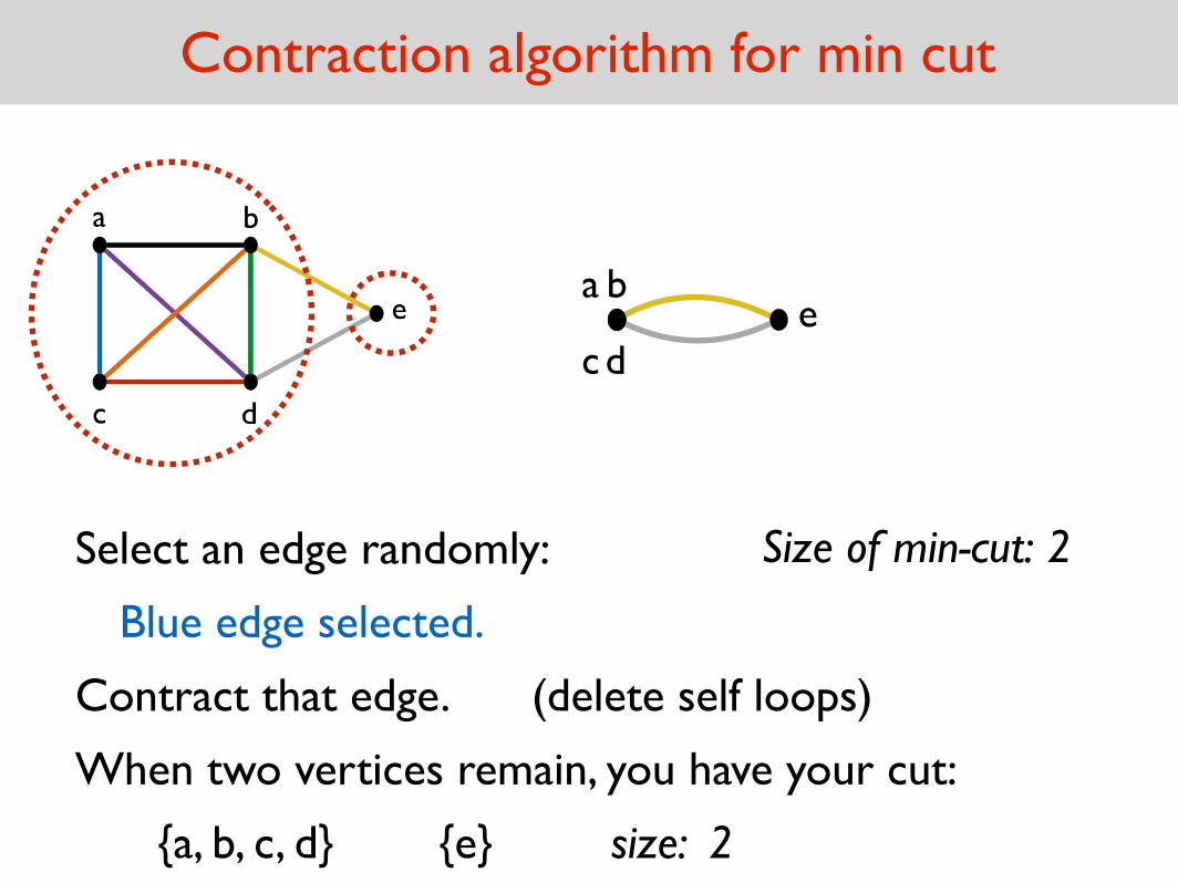
Contraction algorithm for min cut
Blue edge selected.
Contract that edge.
When two vertices remain, you have your cut:
{a, b, c, d} {e} size: 2
(delete self loops)
Size of min-cut: 2Select an edge randomly:
a
c
b
e
d
Contraction algorithm for min cut
Green edge selected.
Contract that edge. (delete self loops)
Size of min-cut: 2Select an edge randomly:
a
c
be
d
Contraction algorithm for min cut
Green edge selected.
Contract that edge. (delete self loops)
Size of min-cut: 2Select an edge randomly:
a
c
be
d
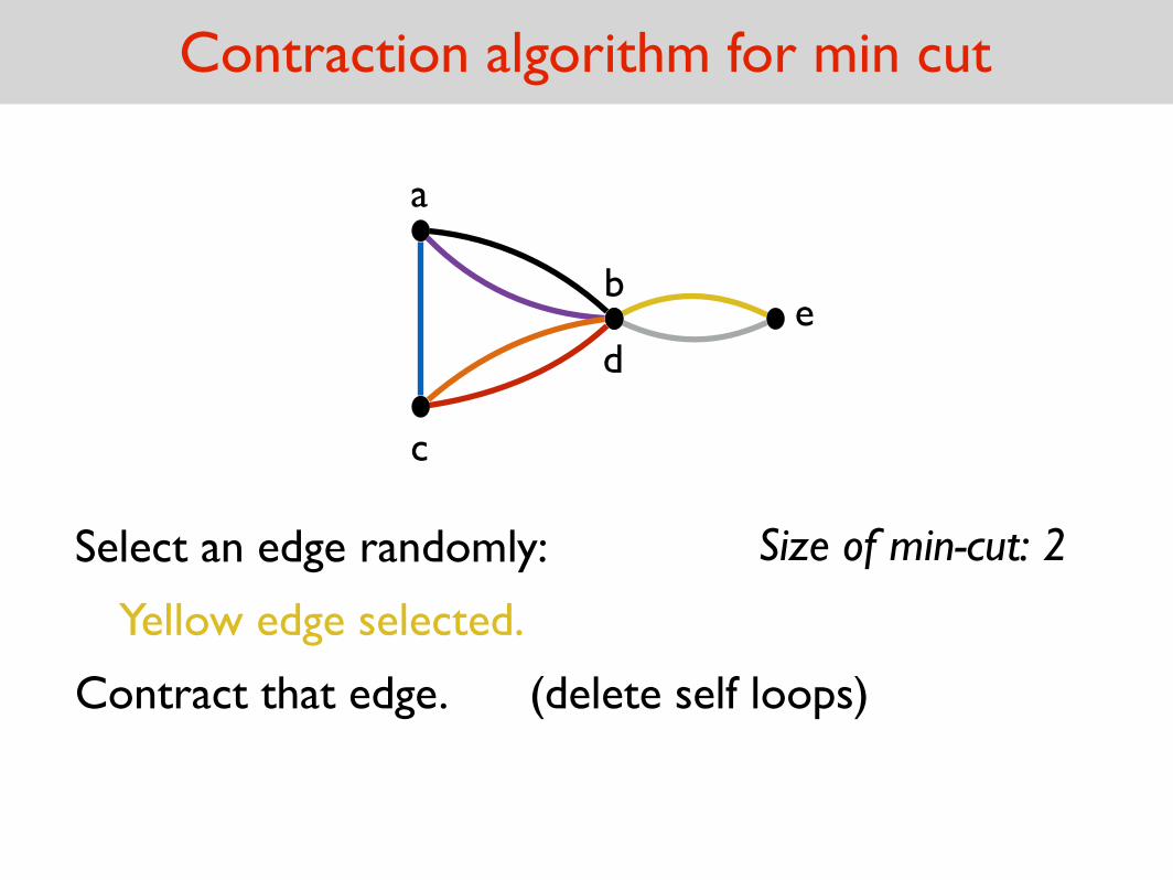
Contraction algorithm for min cut
Yellow edge selected.
Contract that edge. (delete self loops)
Size of min-cut: 2Select an edge randomly:
a
c
be
d
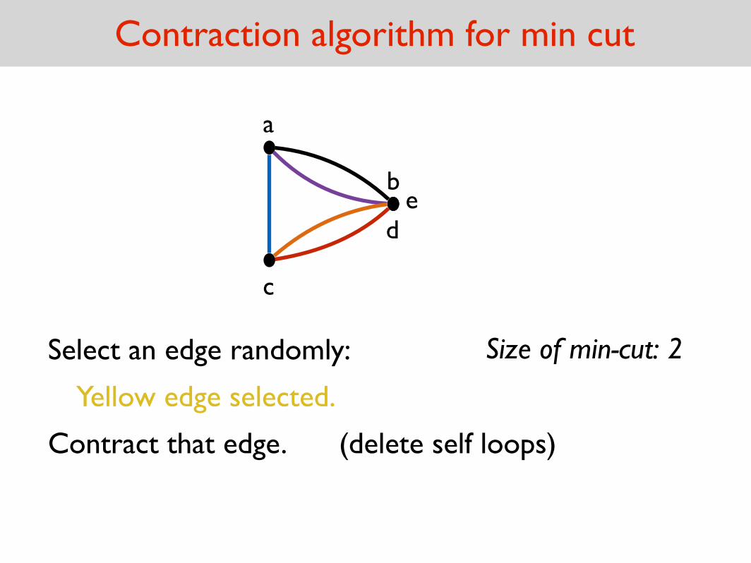
Contraction algorithm for min cut
Yellow edge selected.
Contract that edge. (delete self loops)
Size of min-cut: 2Select an edge randomly:
a
c
be
d
Contraction algorithm for min cut
Red edge selected.
Contract that edge. (delete self loops)
Size of min-cut: 2Select an edge randomly:
a
c
be
d
Contraction algorithm for min cut
Red edge selected.
Contract that edge. (delete self loops)
Size of min-cut: 2Select an edge randomly:
a
c
be
d
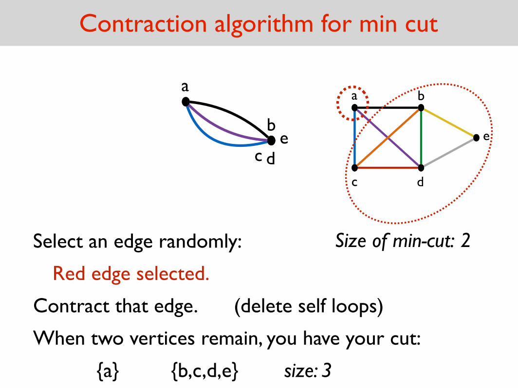
Contraction algorithm for min cut
Red edge selected.
Contract that edge.
When two vertices remain, you have your cut:
{a} {b,c,d,e} size: 3
(delete self loops)
Size of min-cut: 2Select an edge randomly:
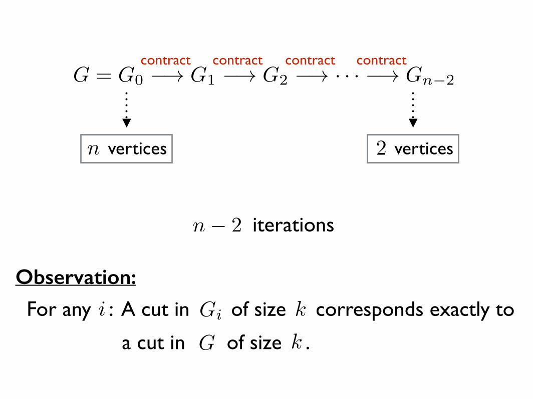
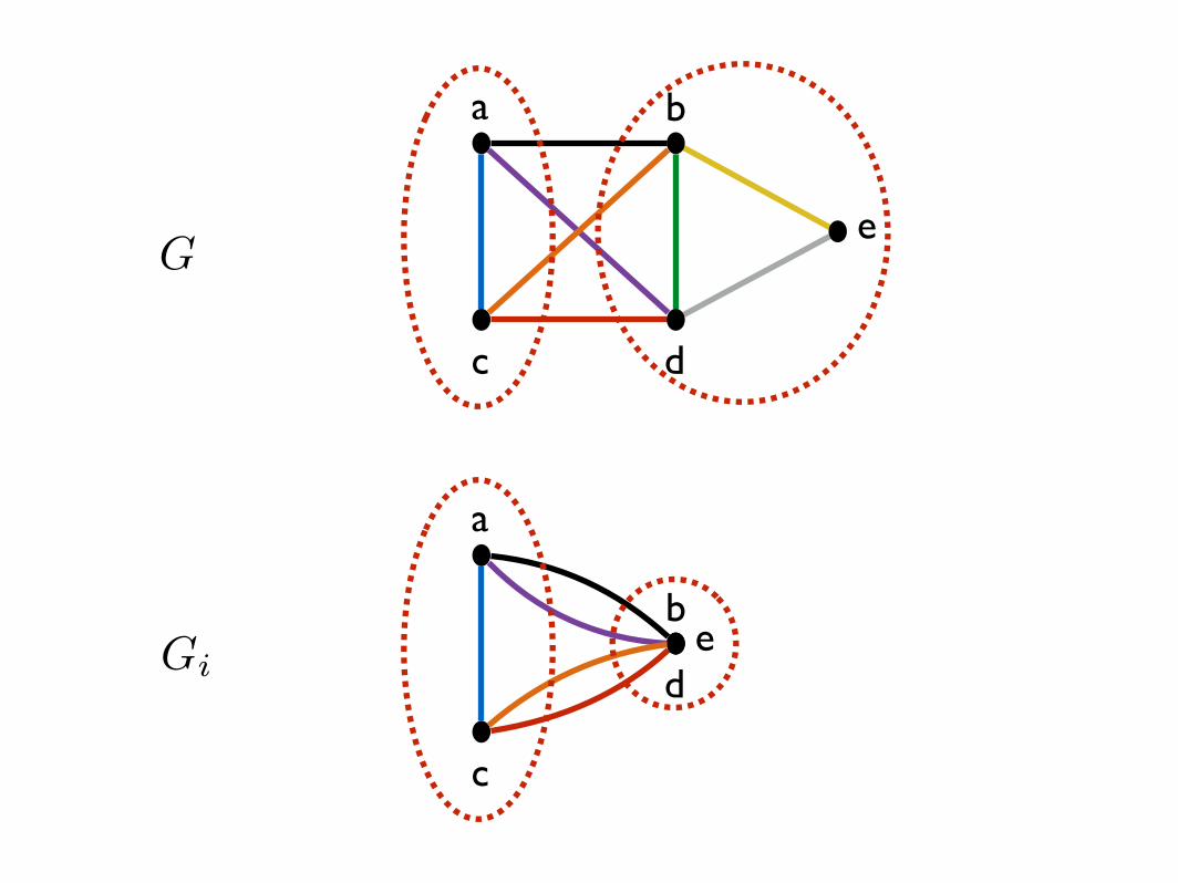
G = G0 �! G1 �! G2 �! · · · �! Gn�2
verticesn vertices2
contract contract contract contract
n� 2 iterations
For any : A cut in of size corresponds exactly to Gi k
a cut in of size .kG
i
Observation:
a
c
be
dGi
a
c
b
e
d
G
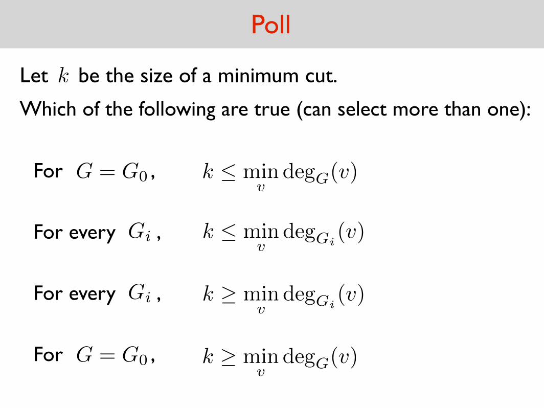
Poll
Let be the size of a minimum cut.k
Which of the following are true (can select more than one):
For every ,Gi k minv
degGi(v)
For ,G = G0 k minv
degG(v)
For every ,Gi
For ,G = G0 k � minv
degG(v)
k � minv
degGi(v)
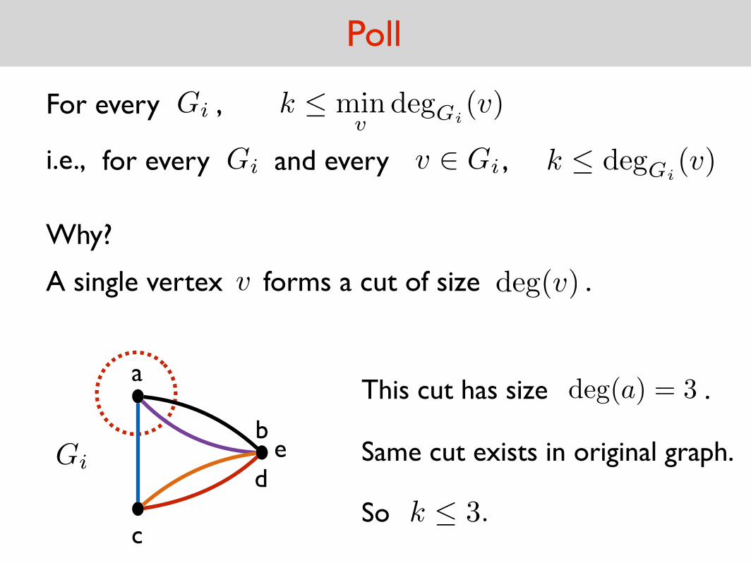
Poll
For every ,Gi k minv
degGi(v)
i.e., for every and every ,Gi v 2 Gi k degGi(v)
Why?
Same cut exists in original graph.
This cut has size .deg(a) = 3
A single vertex forms a cut of size .v deg(v)
k 3.So
a
c
be
dGi

Contraction algorithm for min cut
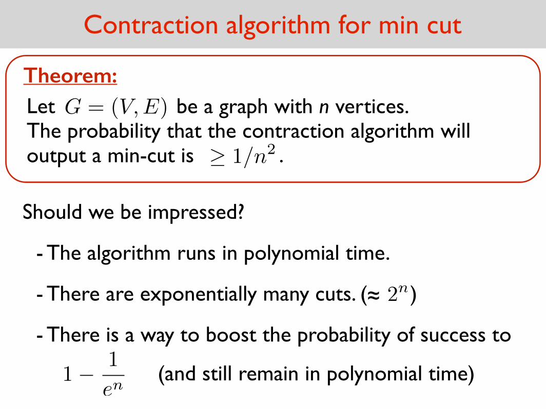
Should we be impressed?
- The algorithm runs in polynomial time.
- There are exponentially many cuts. (~ )2n~
- There is a way to boost the probability of success to
1� 1
en(and still remain in polynomial time)
Let be a graph with n vertices. The probability that the contraction algorithm will output a min-cut is .
Theorem:G = (V,E)
� 1/n2
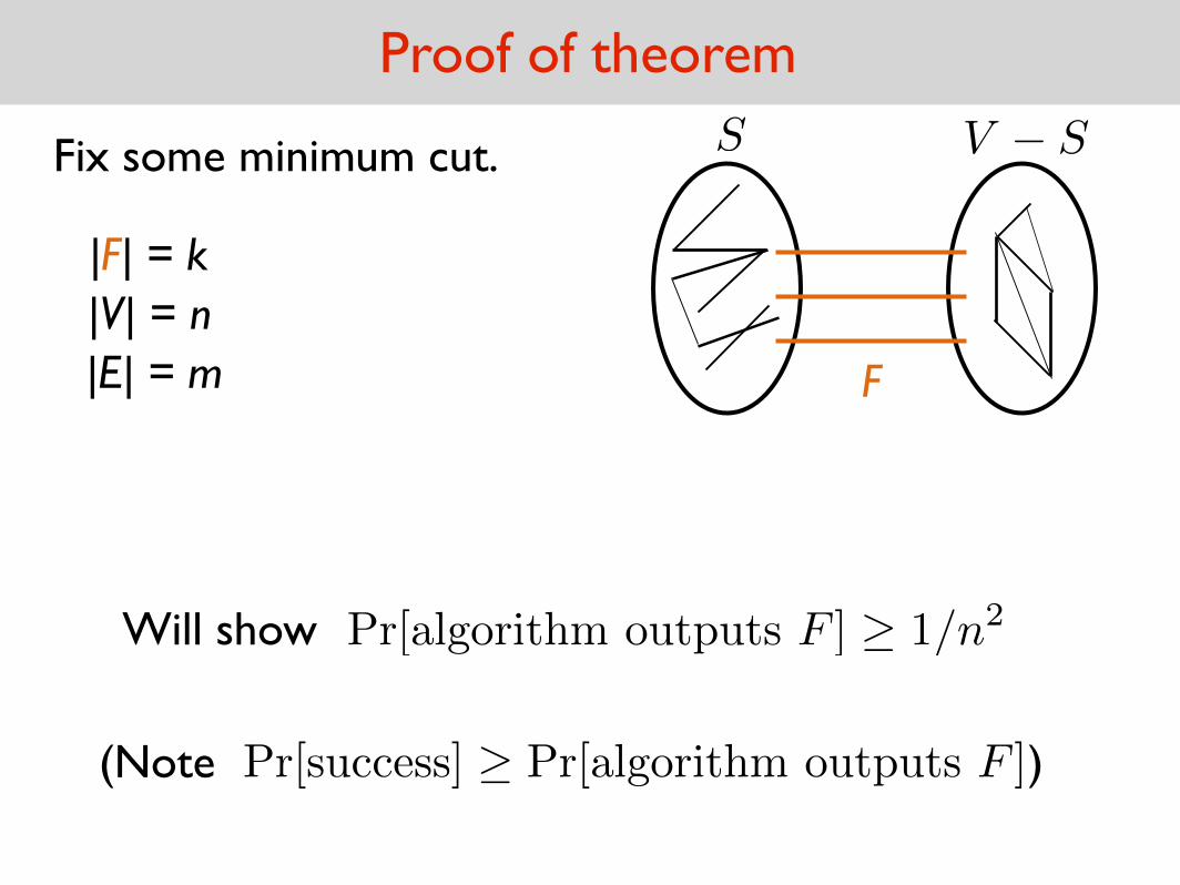
Proof of theorem
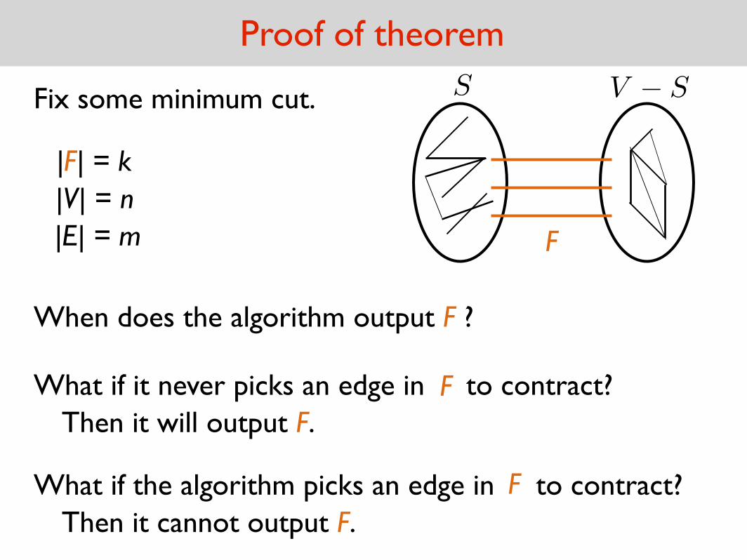
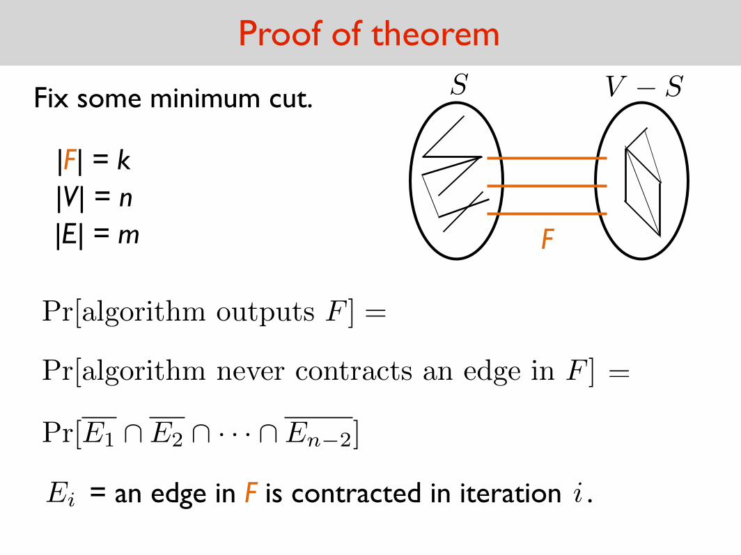
Fix some minimum cut. S V � S
F
|F| = k|V| = n|E| = m
Pr[algorithm outputs F ] � 1/n2Will show
(Note )Pr[success] � Pr[algorithm outputs F ]
Proof of theorem
Fix some minimum cut. S V � S
F
When does the algorithm output F ?
What if the algorithm picks an edge in to contract?FThen it cannot output F.
What if it never picks an edge in to contract?FThen it will output F.
|F| = k|V| = n|E| = m
Proof of theorem
Pr[algorithm outputs F ] =
Pr[algorithm never contracts an edge in F ]
= an edge in F is contracted in iteration .Ei i
Pr[E1 \ E2 \ · · · \ En�2]
=
Fix some minimum cut. S V � S
F
|F| = k|V| = n|E| = m
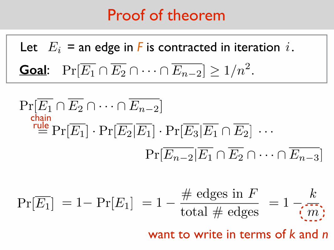
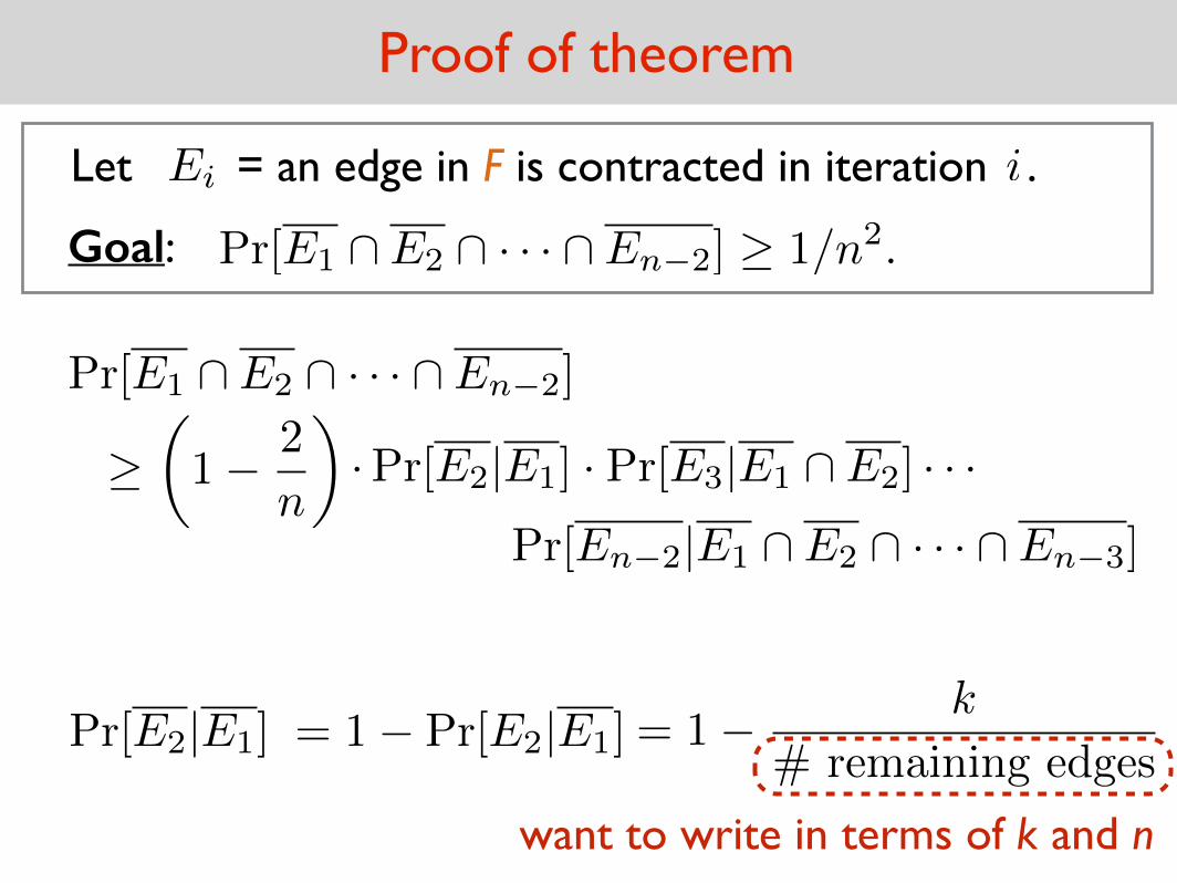
Let = an edge in F is contracted in iteration .Ei i
Proof of theorem
Goal:
Pr[E1 \ E2 \ · · · \ En�2]
= Pr[E1] · Pr[E2|E1] · Pr[E3|E1 \ E2]
Pr[En�2|E1 \ E2 \ · · · \ En�3]
· · ·
Pr[E1 \ E2 \ · · · \ En�2] � 1/n2.
want to write in terms of k and n
chainrule
Pr[E1] Pr[E1]= 1�= 1� # edges in F
total # edges
= 1� k
m
Proof of theorem
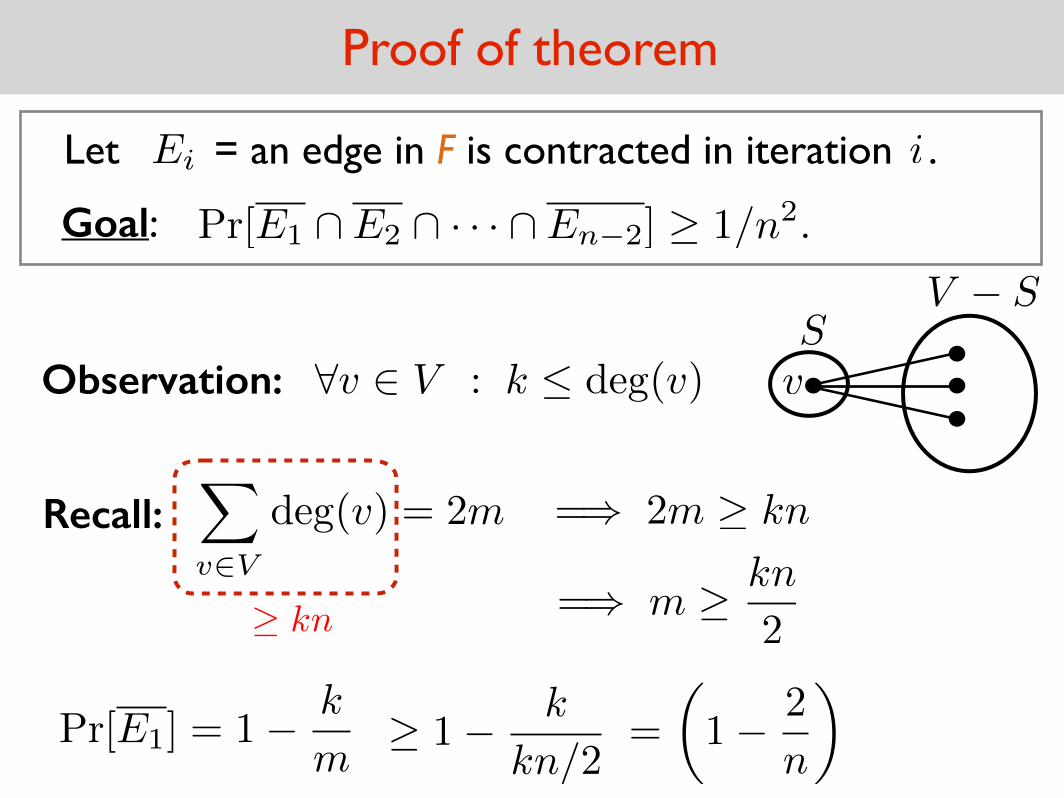
Recall: X
v2V
deg(v) = 2m =) 2m � kn
Let = an edge in F is contracted in iteration .Ei
Goal: Pr[E1 \ E2 \ · · · \ En�2] � 1/n2.
Observation: 8v 2 V : k deg(v)S
V � S
v
i
� kn =) m � kn
2
Pr[E1] = 1� k
m=
✓1� 2
n
◆� 1� k
kn/2
Proof of theorem
Pr[E1 \ E2 \ · · · \ En�2]
Pr[En�2|E1 \ E2 \ · · · \ En�3]
·Pr[E2|E1] · Pr[E3|E1 \ E2] · · ·�✓1� 2
n
◆
Pr[E2|E1] = 1� Pr[E2|E1]= 1� k
# remaining edges
want to write in terms of k and n
Let = an edge in F is contracted in iteration .Ei
Goal: Pr[E1 \ E2 \ · · · \ En�2] � 1/n2.
i
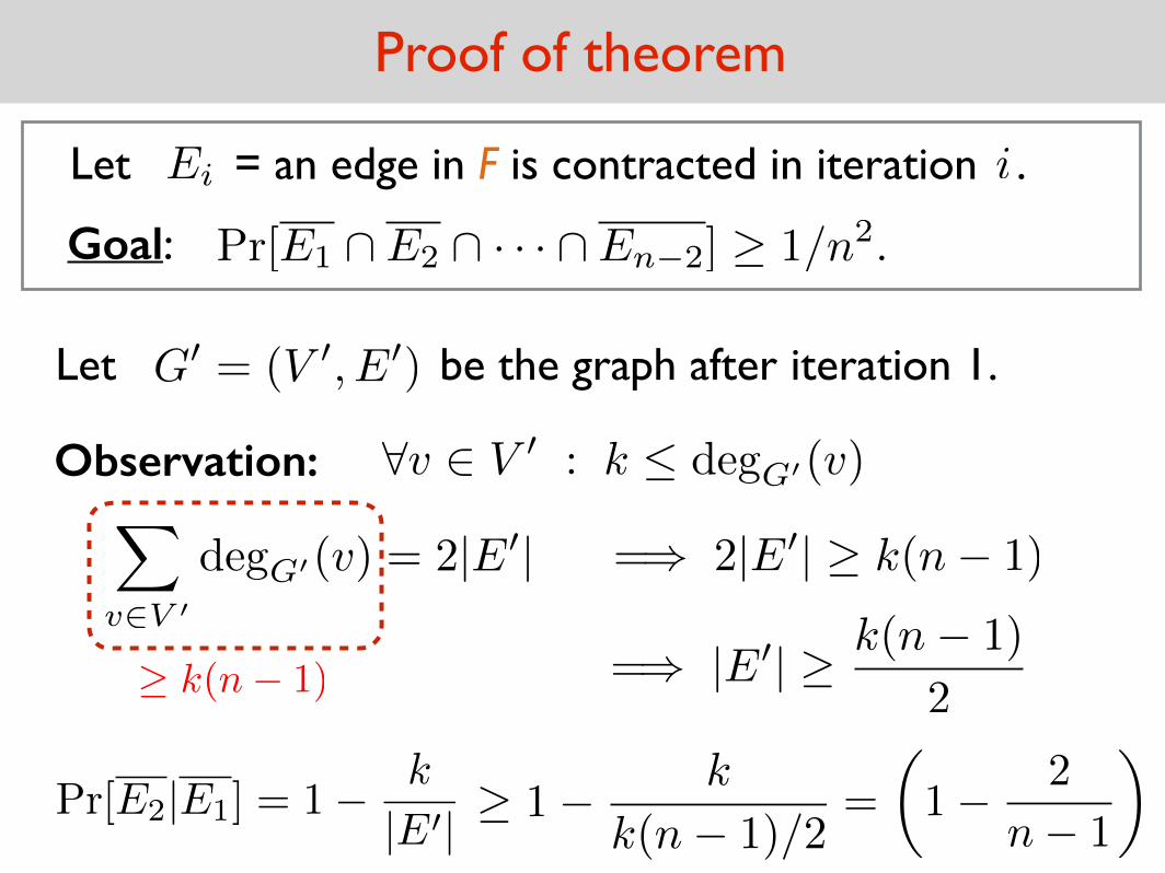
Proof of theorem
Let = an edge in F is contracted in iteration .Ei
Goal: Pr[E1 \ E2 \ · · · \ En�2] � 1/n2.
i
Let be the graph after iteration 1. G0 = (V 0, E0)
Observation: 8v 2 V 0 : k degG0(v)X
v2V 0
degG0(v) = 2|E0|
� k(n� 1)
=) 2|E0| � k(n� 1)
=) |E0| � k(n� 1)
2
Pr[E2|E1] = 1� k
|E0| =
✓1� 2
n� 1
◆� 1� k
k(n� 1)/2
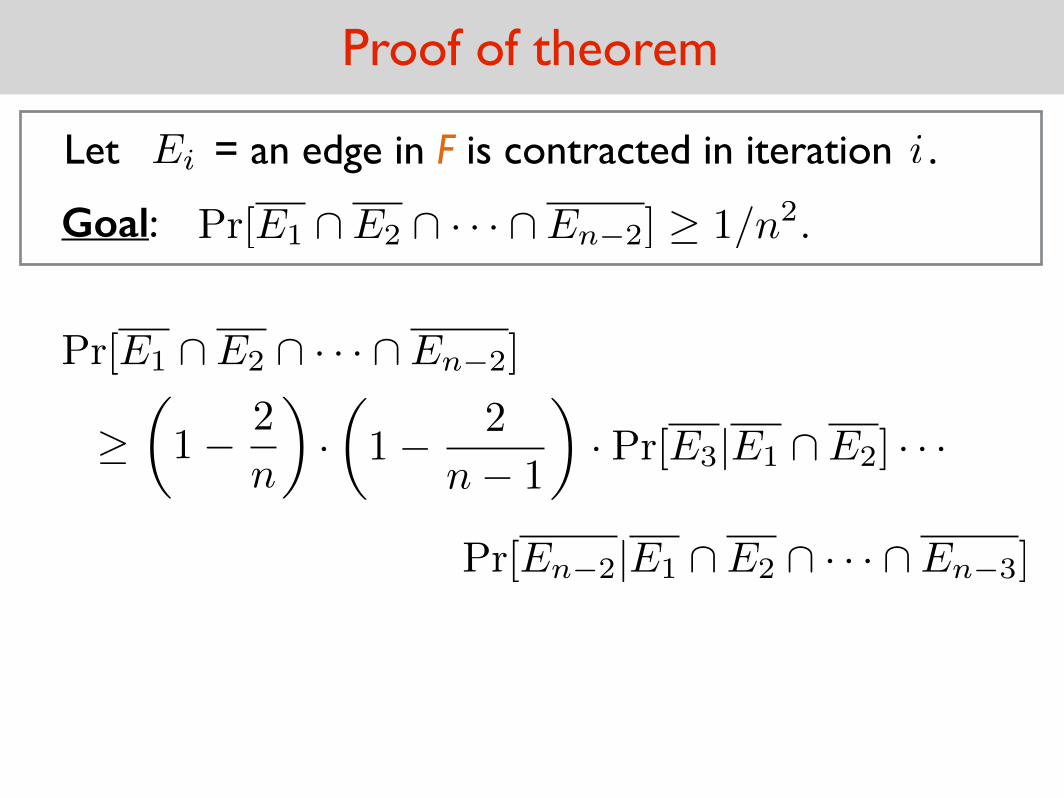
Proof of theorem
Pr[E1 \ E2 \ · · · \ En�2]
Pr[En�2|E1 \ E2 \ · · · \ En�3]
�✓1� 2
n
◆·✓1� 2
n� 1
◆· Pr[E3|E1 \ E2] · · ·
Let = an edge in F is contracted in iteration .Ei
Goal: Pr[E1 \ E2 \ · · · \ En�2] � 1/n2.
i
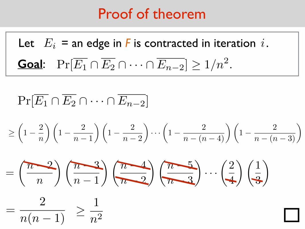
Proof of theorem
Pr[E1 \ E2 \ · · · \ En�2]
Let = an edge in F is contracted in iteration .Ei
Goal: Pr[E1 \ E2 \ · · · \ En�2] � 1/n2.
i
�✓1� 2
n
◆✓1� 2
n� 1
◆✓1� 2
n� 2
◆· · ·
✓1� 2
n� (n� 4)
◆✓1� 2
n� (n� 3)
◆
=
✓n� 2
n
◆✓n� 3
n� 1
◆✓n� 4
n� 2
◆✓n� 5
n� 3
◆· · ·
✓2
4
◆✓1
3
◆
=2
n(n� 1)� 1
n2
Contraction algorithm for min cut
Should we be impressed?
- The algorithm runs in polynomial time.
- There are exponentially many cuts. (~ )2n~
- There is a way to boost the probability of success to
1� 1
en(and still remain in polynomial time)
Let be a graph with n vertices. The probability that the contraction algorithm will output a min-cut is .
Theorem:G = (V,E)
� 1/n2
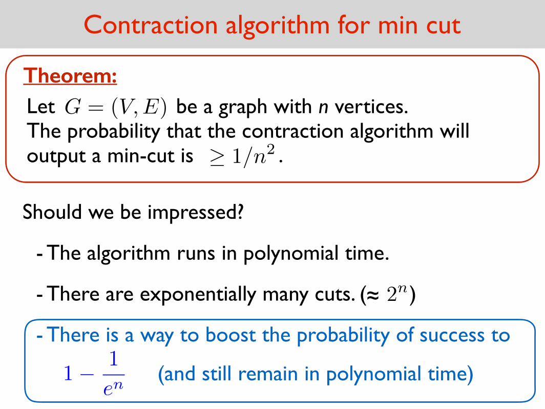
Contraction algorithm for min cut
Should we be impressed?
- The algorithm runs in polynomial time.
- There are exponentially many cuts. (~ )2n~
- There is a way to boost the probability of success to
(and still remain in polynomial time)1� 1
en
Theorem:Let be a graph with n vertices. The probability that the contraction algorithm will output a min-cut is .
Theorem:G = (V,E)
� 1/n2
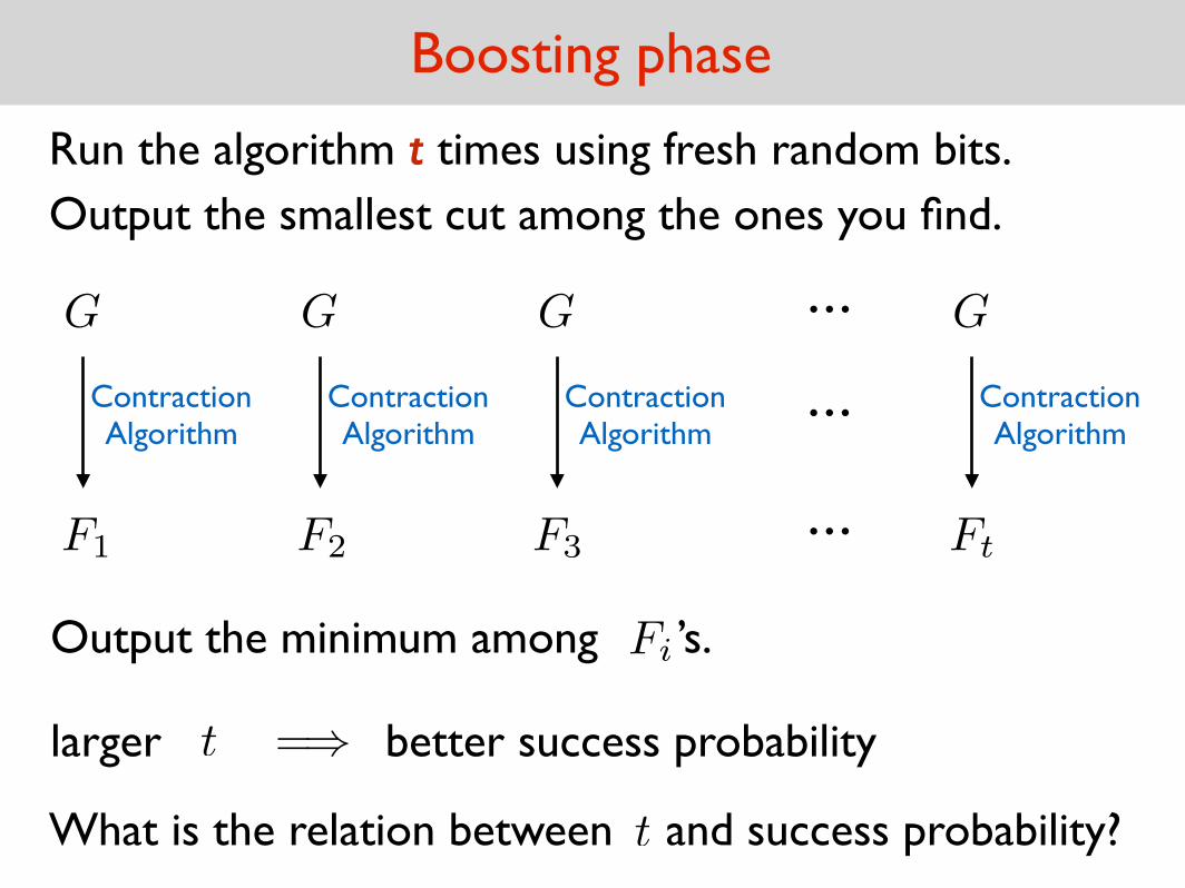
Boosting phase
Run the algorithm t times using fresh random bits.Output the smallest cut among the ones you find.
G G G G
ContractionAlgorithm
ContractionAlgorithm
ContractionAlgorithm
ContractionAlgorithm
…
…
…F1 F2 FtF3
Output the minimum among ’s.Fi
larger better success probabilityt =)
What is the relation between and success probability?t
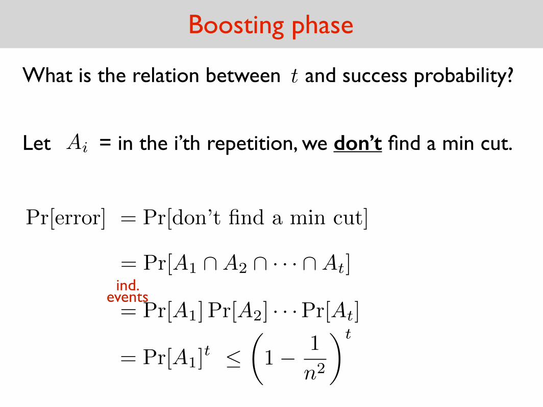
Boosting phase
Let = in the i’th repetition, we don’t find a min cut. Ai
= Pr[A1] Pr[A2] · · ·Pr[At]
= Pr[A1]t
✓1� 1
n2
◆t
What is the relation between and success probability?t
Pr[error]
= Pr[A1 \A2 \ · · · \At]ind.
events
= Pr[don’t find a min cut]
Boosting phase
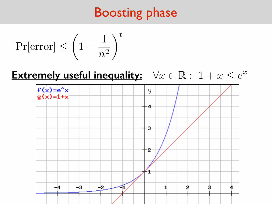
Pr[error] ✓1� 1
n2
◆t
Extremely useful inequality: 8x 2 R : 1 + x e
x
Boosting phase
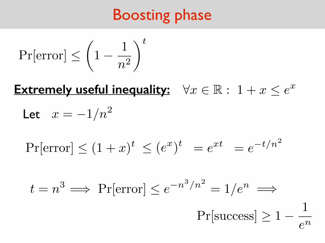
Pr[error] ✓1� 1
n2
◆t
Extremely useful inequality: 8x 2 R : 1 + x e
x
x = �1/n2Let
t = n3=) Pr[error] e�n3/n2
= 1/en
(ex)t = ext = e�t/n2
Pr[success] � 1� 1
en
=)
Pr[error] (1 + x)
t
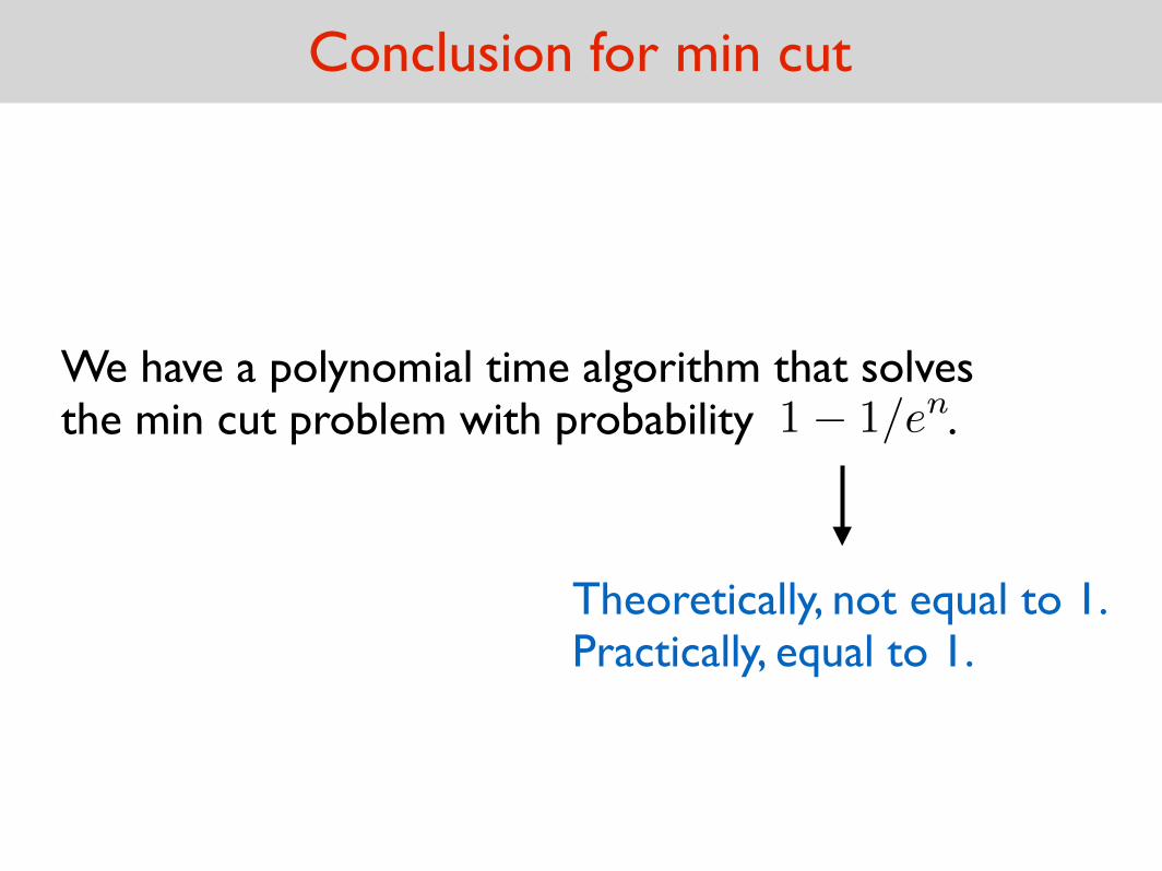
Conclusion for min cut
We have a polynomial time algorithm that solves the min cut problem with probability .1� 1/en
Theoretically, not equal to 1.Practically, equal to 1.
We can boost the success probability of Monte Carlo algorithms via repeated trials.
Important Note
Boosting is not specific to Min-cut algorithm.
Example of a Las Vegas Algorithm: Quicksort
Doesn’t gamble with correctness. Gambles with running time.
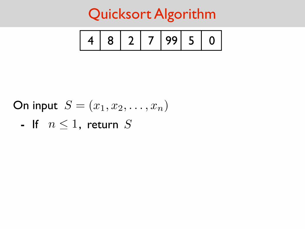
Quicksort Algorithm
8 2 7 99 5 04
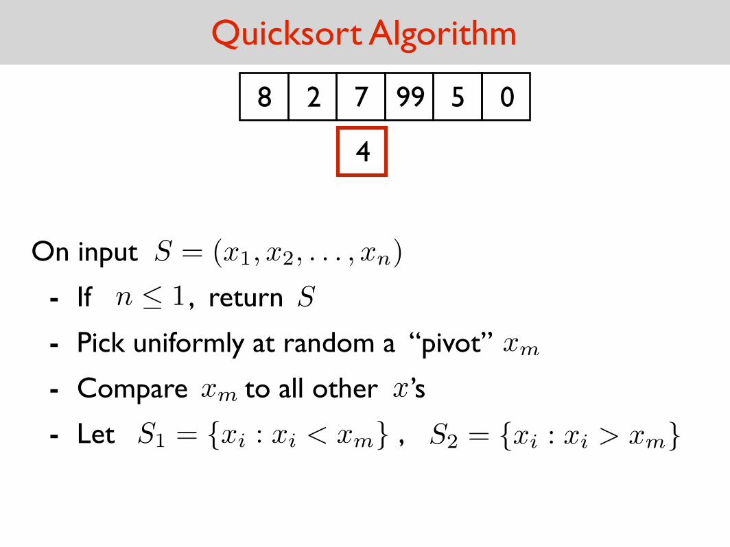
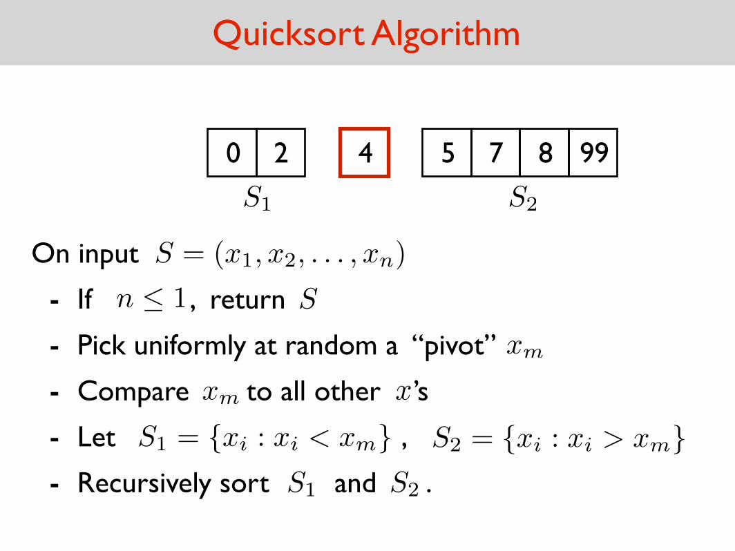
On input S = (x1, x2, . . . , xn)
If , return n 1 S-
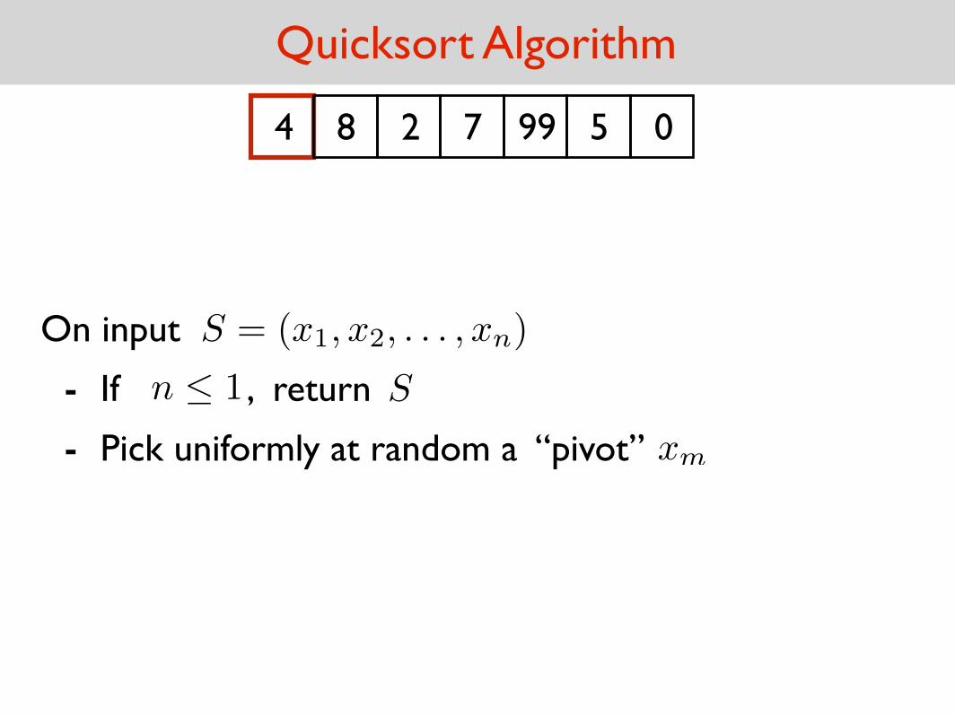
Quicksort Algorithm
8 2 7 99 5 04
On input S = (x1, x2, . . . , xn)
If , return n 1 S
Pick uniformly at random a “pivot” xm
-
-
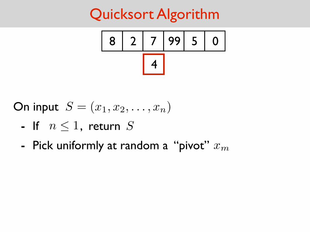
Quicksort Algorithm
8 2 7 99 5 0
4
On input S = (x1, x2, . . . , xn)
If , return n 1 S-
Pick uniformly at random a “pivot” xm-
Quicksort Algorithm
8 2 7 99 5 0
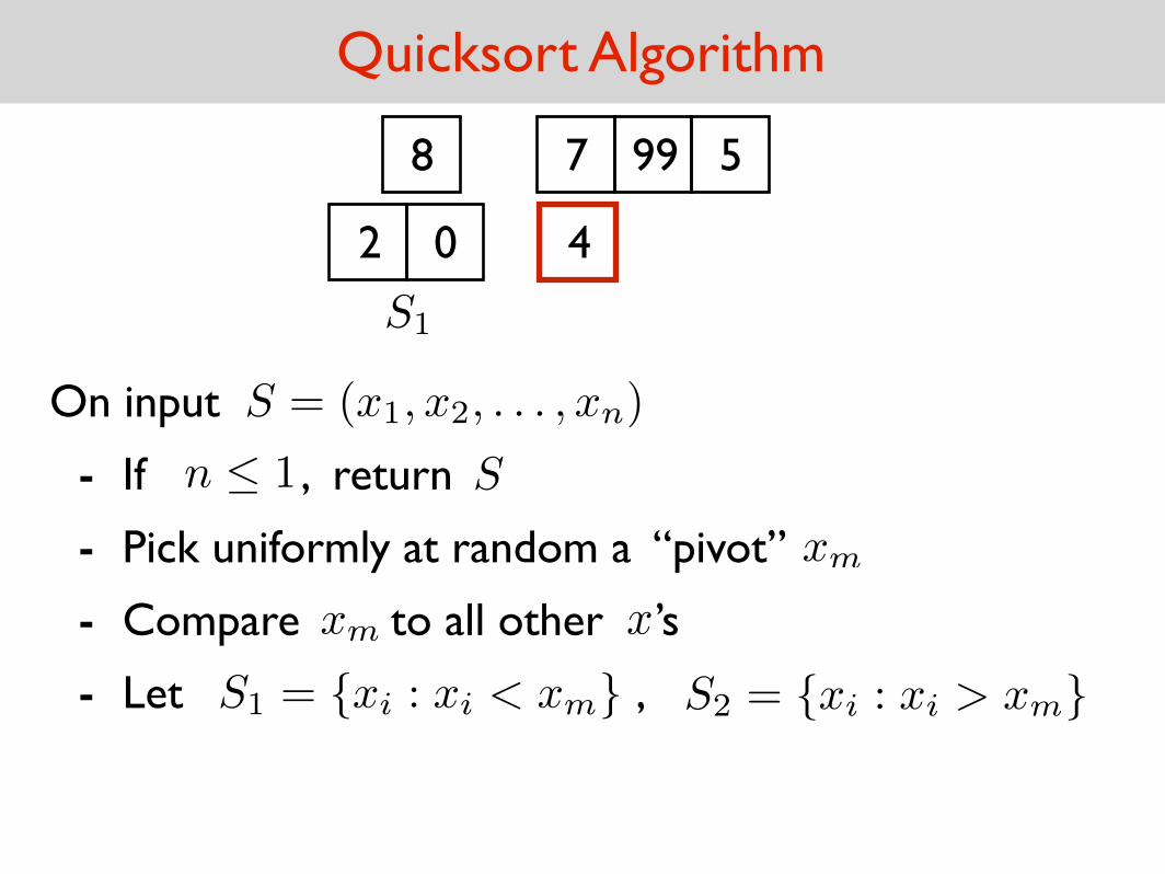
On input S = (x1, x2, . . . , xn)
If , return n 1 S
Compare to all other ’s xm x
Let ,S1 = {xi : xi < xm}S2 = {xi : xi > xm}
-
-
-
4
Pick uniformly at random a “pivot” xm-
Quicksort Algorithm
8 7 99 5
On input S = (x1, x2, . . . , xn)
If , return n 1 S
Compare to all other ’s xm x
Let ,S1 = {xi : xi < xm}S2 = {xi : xi > xm}
-
-
-
42 0
S1
Pick uniformly at random a “pivot” xm-
Quicksort Algorithm
8 7 99 5
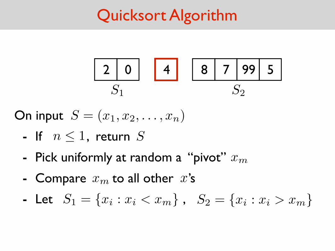
On input S = (x1, x2, . . . , xn)
If , return n 1 S
Compare to all other ’s xm x
Let ,S1 = {xi : xi < xm}S2 = {xi : xi > xm}
-
-
-
42 0
S1 S2
Pick uniformly at random a “pivot” xm-
Quicksort Algorithm
8 7 99 5
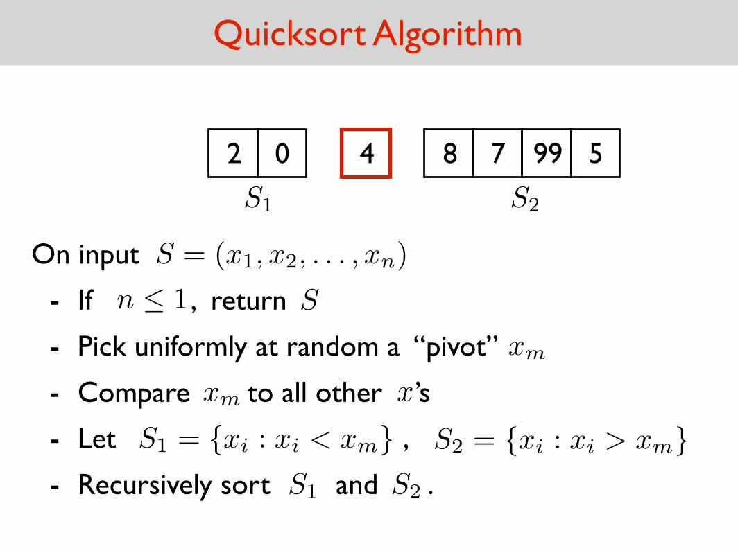
On input S = (x1, x2, . . . , xn)
If , return n 1 S
Compare to all other ’s xm x
Let ,S1 = {xi : xi < xm}S2 = {xi : xi > xm}
-
-
-
42 0
S1 S2
Recursively sort and .S1 S2-
Pick uniformly at random a “pivot” xm-
Quicksort Algorithm
5 7 8 99
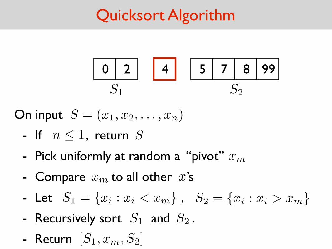
On input S = (x1, x2, . . . , xn)
If , return n 1 S
Compare to all other ’s xm x
Let ,S1 = {xi : xi < xm}S2 = {xi : xi > xm}
-
-
-
40 2
S1 S2
Recursively sort and .S1 S2-
Pick uniformly at random a “pivot” xm-
Quicksort Algorithm
5 7 8 99
On input S = (x1, x2, . . . , xn)
If , return n 1 S
Compare to all other ’s xm x
Let ,S1 = {xi : xi < xm}S2 = {xi : xi > xm}
-
-
-
40 2
S1 S2
Recursively sort and .S1 S2-
Return [S1, xm, S2]-
Pick uniformly at random a “pivot” xm-
Quicksort Algorithm
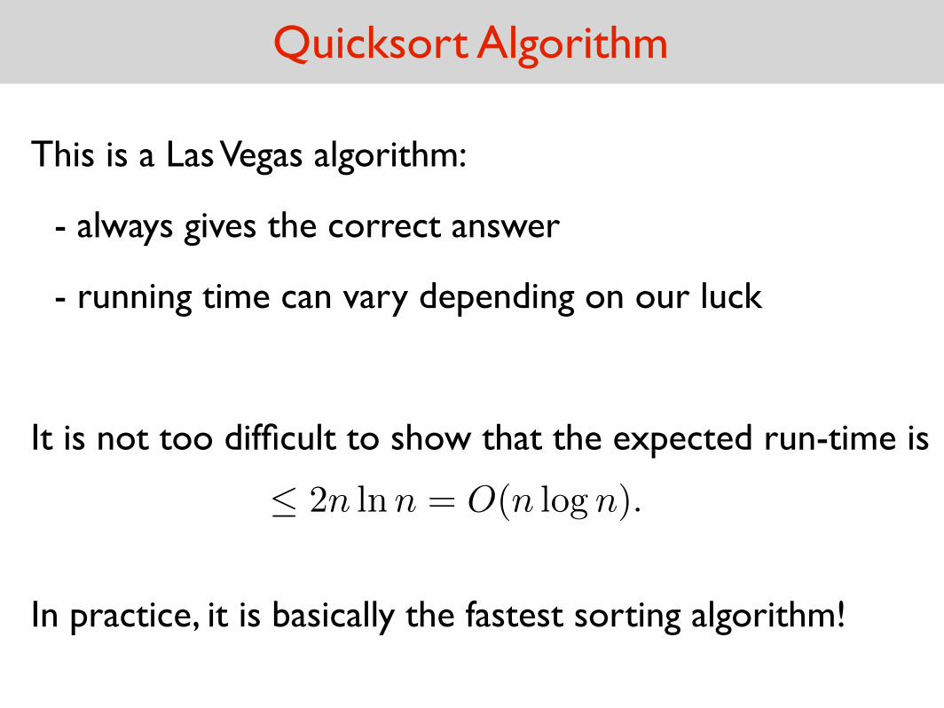
This is a Las Vegas algorithm:
- always gives the correct answer
- running time can vary depending on our luck
It is not too difficult to show that the expected run-time is
2n lnn = O(n log n).
In practice, it is basically the fastest sorting algorithm!
Final remarks
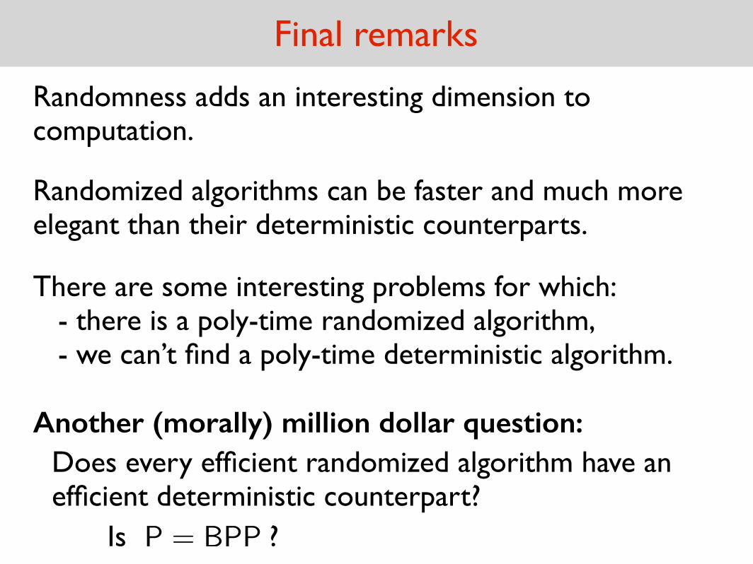
Another (morally) million dollar question:Does every efficient randomized algorithm have an efficient deterministic counterpart?
P = BPPIs ?
Randomized algorithms can be faster and much more elegant than their deterministic counterparts.
There are some interesting problems for which: - there is a poly-time randomized algorithm, - we can’t find a poly-time deterministic algorithm.
Randomness adds an interesting dimension to computation.