15. NEURAL NETWORKS

15.1 Introduction to The Chapter

In this chapter, we provide a new perspective into neural networks, bothfeedforward and feedback networks. In section 15.2, we provide a small primeron neural networks. In addition to providing necessary details (that will be ofuse to those who are not familiar neural networks) in a concise manner, we try toremove the mystery and hype surrounding these networks and try to look atthem in a more critical and objective way. Thus, we concentrate on what theycan really do, how they do it, what are the advantages and disadvantages, etc.One key aspect of neural networks we try to highlight in this and the nextsection is that they represent special classes of nonlinear networks, and hencewe can learn quite a lot by understanding nonlinear networks and theirdynamics. In section 15.3, we consider recurrent neural networks (RNNs), orneural networks with internal feedback, and discuss some of the well-knownmodels. In the case of recurrent neural networks, stability, or the lack of it, is amajor concern, and we discuss some of the existing approaches to prove thestability of RNNs. This section highlights the slow progress in the design ofRNNs due to the lack of structured methods to obtain RNN architectures withguaranteed stability property and the problems in training such networks. Insection 15.4, we discuss a new approach based on the building block concept(seen in earlier chapters for designing complex, stable nonlinear networks) toobtain new and complex RNN architectures and develop training or learningalgorithms. We also show that existing RNN architectures can be derived byplacing specific constraints on the architectures obtained using the buildingblock approach. We also indicate that in RNN architectures, no energy functionis being minimized, but a situation of power balance (between sources andsinks) is reached.

15.2 Neural Networks: A Primer

15.2.1 Basic Terminology and Functions

In chapter #1 and later chapters, we argued that a system could be viewed asperforming a mapping from an input domain to an output domain. Here, we willlook at neural networks from the same perspective. We start the discussion bylooking at the different levels (in the order of increasing complexity) ofsignal/information processing described in chapter # 1.

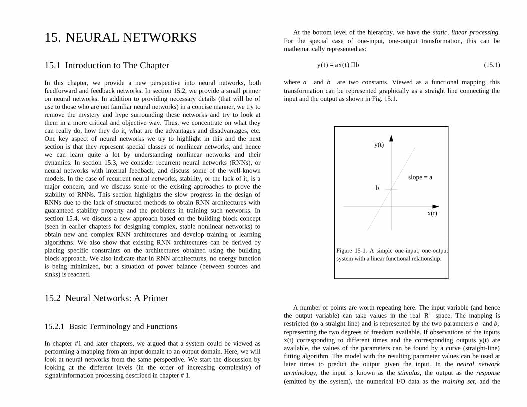
At the bottom level of the hierarchy, we have the static, linear processing.For the special case of one-input, one-output transformation, this can bemathematically represented as:

y(t) = ax(t) + b (15.1)

where a and b are two constants. Viewed as a functional mapping, thistransformation can be represented graphically as a straight line connecting theinput and the output as shown in Fig. 15.1.

A number of points are worth repeating here. The input variable (and hencethe output variable) can take values in the real R1 space. The mapping isrestricted (to a straight line) and is represented by the two parameters a and b,representing the two degrees of freedom available. If observations of the inputsx(t) corresponding to different times and the corresponding outputs y(t) areavailable, the values of the parameters can be found by a curve (straight-line)fitting algorithm. The model with the resulting parameter values can be used atlater times to predict the output given the input. In the neural networkterminology, the input is known as the stimulus, the output as the response(emitted by the system), the numerical I/O data as the training set, and the

x(t)

y(t)

b

slope = a

Figure 15-1. A simple one-input, one-outputsystem with a linear functional relationship.

parameter estimation process as learning or training. In this particular example,both the samples of the stimulus and the response are assumed to be availablefor training. Such learning or training process is known as supervised orteacher-based learning. We will see later examples of the other learningcategory known as unsupervised learning, also known as self-organization.

An important observation that can be made from this simple single input,single output system is that the degree of freedom is restricted to two {or someconstant for the general case} for linear processing and cannot be increased anyfurther. In other words, any linear representation involving more than twovariables {or degrees of freedom} can be reduced to the representation involvingonly two variables. This is not so for nonlinear processing, which makes it morecomplicated and interesting.

By relaxing the linearity constraint, we obtain the next level of processing---static, nonlinear processing. Depending upon the nonlinear primitive(s)employed, we can obtain different mathematical representations. For example,in the simple one-input, one-output case we could have:

y(t) = a i xi (t)

i=0

M

∑ (15.2)

or

y(t) = b i tanh[c i xi (t)]i=0

N

∑ (15.3)

The first expression simply involves a polynomial (of order M)representation with the various powers of the inputs as the nonlinear primitivesor as the basis of representation, whereas the second involves weightedtranscendal functions of the scaled inputs. The coefficients a i (i = 0 to M) and

b i , c i (i = 0 to N) represent the degrees of freedom available in modeling the

given system using the two representations.As we noted in chapter # 4, and as the two examples above illustrate, the

leap from linear to nonlinear is not that simple. The choice for nonlinearprimitives is unlimited. The nonlinear primitives and nonlinear representationshave to be chosen to represent the mapping process properly1. That is, onerepresentation may be good for one set of systems stimulated by a particular setof inputs, but may fail miserably with other sets of systems and or inputs even ifthe degrees of freedom are increased considerably. Further, the training data hasto be a good representation of the stimuli seen by the system in its past as wellas the inputs that will be seen in the future. Thus, input and output probability

1 We will see shortly how these issues have been resolved in the neural networkarea.

functions play a major role in the approximation (training or learning) process.Though researchers in the neural network area assume the probability functionsare unknown and claim that it need not be known apriori, the conditions thatgood representative data must be available and must be used are very important.

15.2.2 Primitives of Neural Architectures & Feedforward NeuralNetworks

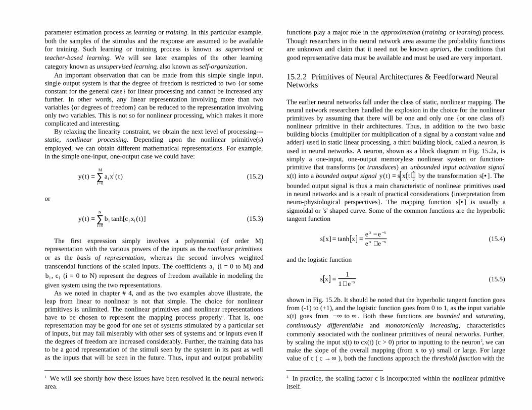
The earlier neural networks fall under the class of static, nonlinear mapping. Theneural network researchers handled the explosion in the choice for the nonlinearprimitives by assuming that there will be one and only one {or one class of}nonlinear primitive in their architectures. Thus, in addition to the two basicbuilding blocks {multiplier for multiplication of a signal by a constant value andadder} used in static linear processing, a third building block, called a neuron, isused in neural networks. A neuron, shown as a block diagram in Fig. 15.2a, issimply a one-input, one-output memoryless nonlinear system or function-primitive that transforms (or transduces) an unbounded input activation signalx(t) into a bounded output signal y(t) = s x t( )[ ] by the transformation s[•]. The

bounded output signal is thus a main characteristic of nonlinear primitives usedin neural networks and is a result of practical considerations {interpretation fromneuro-physiological perspectives}. The mapping function s[•] is usually asigmoidal or 's' shaped curve. Some of the common functions are the hyperbolictangent function

s[x] = tanh x[ ] =e x − e −x

e x + e −x (15.4)

and the logistic function

s x[ ] =1

1+ e−x (15.5)

shown in Fig. 15.2b. It should be noted that the hyperbolic tangent function goesfrom (-1) to (+1), and the logistic function goes from 0 to 1, as the input variablex(t) goes from −∞ to ∞ . Both these functions are bounded and saturating,

continuously differentiable and monotonically increasing, characteristicscommonly associated with the nonlinear primitives of neural networks. Further,by scaling the input x(t) to cx(t) (c > 0) prior to inputting to the neuron2, we canmake the slope of the overall mapping (from x to y) small or large. For largevalue of c ( c →∞ ), both the functions approach the threshold function with the

2 In practice, the scaling factor c is incorporated within the nonlinear primitiveitself.

output of {0, 1} or {-1, 1} as shown in the Fig. 15.2b. Thus the output of theneurons becomes binary or bipolar. A neuron whose output signal approachesthe value one might be considered a winning neuron where as the one whosesignal level remains near zero (or minus one) a losing neuron.

We indicated earlier that the choice of the nonlinear primitives is crucial forproper modeling of a given nonlinear mapping. Thus, we may wonder whateffect fixing the nonlinear primitives as neurons will have on the modeling andwhat the neural researchers have to say about this. Neural network researchersargue that the use of very large number {approaching millions and more} of thesame nonlinearities is sufficient to model any kind of nonlinear mapping seen inpractice. The key word here is "in practice". We can construct arbitrary

mappings to show that architectures composed of only neurons cannot do the jobof approximation properly. Thus, care has to be exercised in the use of neuralarchitectures, and the one size fit all approach will only lead to failure anddisappointment concerning the real potential of neural networks.

In general, a static neural network architecture3 {also known as feedforwardneural net} is formed from the three primitives mentioned above and fixed biasinputs. Similar to the human brain with roughly 100 billion neurons, it isassumed that a useful artificial neural net or ANN {artificial to differentiate itfrom the real neural nets} will have millions of nonlinear neurons. The neuronsare grouped into different fields {or layers for feedforward nets}, and neurons ina particular field receive, as inputs, the sum of weighted signals from neuronsfrom proceeding fields and bias signals as shown in Fig. 15.3. The summingjunction is known as the synoptic junction, the weights as synoptic weights orsynoptic efficacies {and classified as excitory if the weights are positive and asinhibitory if the weights are negative}, and the matrix consisting of the synopticweights as synoptic matrix or connection matrix. A synoptic function of each

neuron may receive signals from a large number {104 in the case of the human

brain} of neurons from the proceeding field. Thus, the factors that make a neuralnet unique among all static, nonlinear mapping systems are:

1) the use of few primitives or building blocks;2) the use of a large number of the only nonlinear building block, the

neuron;3) the use of very large number of trainable synoptic weights, and4) the use of very large number of interconnections.Referring to Fig. 15.3a of a feedforward neural net, we find a number of

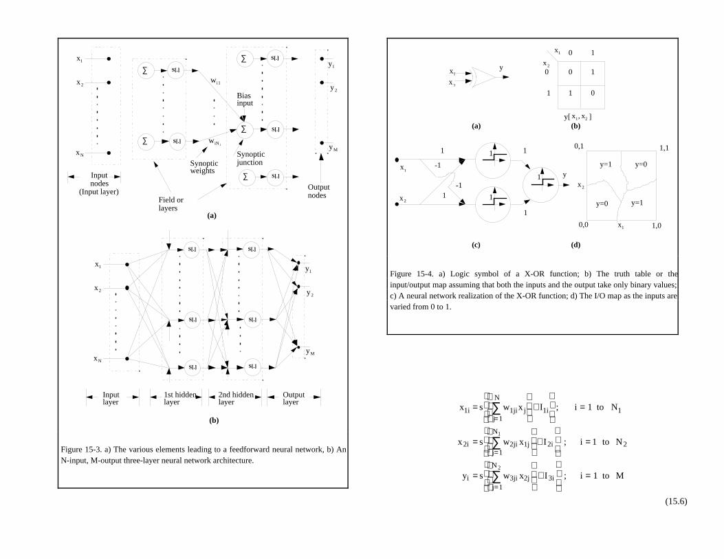
inputs going into the input layer {a distribution terminal}, an output layer and anumber of intermediate layers known as hidden layers. From a nonlinearfunctional mapping perspective, the presence of hidden layers provides thecapability to implement reasonable mappings using the simple & only onenonlinear primitive. In fact, earlier research in neural nets stalled temporarilywhen it was shown that even a simple mapping such as a two input Exclusive-Orproblem {two binary inputs & one binary output as shown in Fig. 15.4} cannotbe implemented using a single layer network. It is now widely accepted that twohidden layer are sufficient for acceptable mapping. As indicated before, theweights are found using I/O data samples and a training procedure. Neuralnetwork researchers term such estimation as model-free estimation as (accordingto them) they do not use a mathematical model describing how systems’ outputsdepend on its inputs. However, considering Fig. 15.3b, where we have shown athree-layer network, the outputs can be written in terms of the inputs as:

3 This definition doesn’t take into consideration that the inputs to this networkmight come from a time-series and updated continuously.

S[.]x(t) y(t)

-8 -4 0 4 8

-0.8

-0.4

0

0.4

0.8

x

Threshold Function

Logistic Function

Sigmoidal Function

(a)

(b)

Figure 15-2. a) The block diagram of neuron, a nonlinear primitive used inneural networks; b) Commonly used characteristics for the neuron.

x1i = s w1jix jj=1

N

∑

+ I1i

; i = 1 to N1

x2i = s w2ji x1jj=1

N1

∑

+ I2i

; i = 1 to N2

yi = s w3ji x2jj=1

N 2

∑

+ I3i

; i = 1 to M

(15.6)

y1

y2

yM

x1

x2

xNS[.]

S[.]

S[.]

S[.]

S[.]

S[.]

Inputlayer

1st hiddenlayer

2nd hiddenlayer

Outputlayer

(b)

Inputnodes

(Input layer)

x1

x2

xN

y1

y2

yM

S[.]

S[.]

∑

∑

S[.]∑

S[.]

S[.]

∑

∑

wi1

wiN i

Biasinput

Field orlayers

SynopticjunctionSynoptic

weights

Outputnodes

(a)

Figure 15-3. a) The various elements leading to a feedforward neural network, b) AnN-input, M-output three-layer neural network architecture.

x1

x2

y

1

1

11

1

-1

-1

1

1

y

x2

x1

(a)

(c)

x2

x1

0

1

0 1

0 1

1 0

(b)y[ x1, x2 ]

x1

x2

0,0 1,0

1,10,1

y=1

y=1

y=0

y=0

(d)

Figure 15-4. a) Logic symbol of a X-OR function; b) The truth table or theinput/output map assuming that both the inputs and the output take only binary values;c) A neural network realization of the X-OR function; d) The I/O map as the inputs arevaried from 0 to 1.

Thus, there is an underlying model involving the various primitives, thoughthe model may be at a micro level. The contention that there is an underlyingmodel becomes more valid in the case of other more complex neural networksas such as recurrent neural networks that we will see shortly. Before we do that,let’s look at possible applications of neural nets and training of FFNN weights.

15.2.3 Implementational Issues

As we learned in the previous subsection, an artificial neural network is formedfrom dense interconnection among a large number of elements taken from a verylimited primitive set. Within that domain, we do have a number of choicesconcerning the signals to be processed, implementational issues, andapplications. The inputs and or the outputs can be continuous signals, digitalsignals, or binary/bipolar signals. The continuous signals can be processed usinganalog, electronics or analog, optical implementation or digital technology usingA/D converters in the front end and D/A converters at the output end. Thedigital signals can be processed using digital hardware based on binary logic.The binary/bipolar signals can be processed using analog or digital architecture.Also, we can either time-multiplex one or few processing units or use amassively parallel architecture. It may be true that the human brain {the trueneural net} performs its tasks using nonlinear, massively parallel, asynchronous{no underlying clock} and feedback architecture. However, some or any ofthese may or may not apply to artificial neural nets depending on how they havebeen designed and implemented. Hence, caution must be exercised whilecoming across such "hyperbole”.

15.2.4 Techniques for Signal Encoding

Another unique property of neural architectures is the technique used for signalencoding. We all know that B-bits (and B channels in an implementationalsense) can be used to uniquely denote 2B symbols and to denote 2B quantizationlevels in a weighted-scheme. Here, the representation is obtained by minimizing(to the lowest level) the number of bits or channels needed in the representation.Of course, such a representation is neither fault tolerant4, nor provides the abilityfor graceful degradation5. In digital computing and communication areas, anaccepted solution to these problems is through the use of error detection andcorrection schemes where we basically add a few more redundant (in aninformation point of view) bits to the codes corresponding to each symbol in asystematic manner. We know that higher the number of bits we add per symbol,the better the error correction / error detection properties will be. For example,

4 Outputs remain unchanged even if some of the parameters change.5 Minimal change in the performance for some changes in the parameters.

the addition of just one bit per symbol code {through the use of bit parityschemes, for example} enable us to detect if an odd number of bits havechanged. Adding one bit alone doesn't help us in detecting the change in an evennumber of bits or help in determining the corrupted bits. We can, of course, addtwo or more bits to have better error detection and correction capability. Neuralarchitectures take this concept to the extreme where B-bits are used to denotejust B symbols or B quantization levels. Such an encoding is know as distributedcoding and leads to a redundant encoding (we will have more than one coderepresenting the same symbol). The redundancy leads to better fault tolerance(deviations in weights for example will have minimal effect on the input/outputmapping), and graceful degradation (removing certain connections for examplewill not drastically change the mapping) properties. Of course, as the number ofchannels and the associated elements have increased enormously, it can beargued that the chances for failure are higher. More on this as we look at theapplications.

15.2.5 Applications of Neural Nets

By constraining the inputs and outputs to special domains (of values), we cangain some knowledge about possible applications for artificial neural nets. Forexample, if both the inputs and outputs are multi-valued (in amplitude ormagnitude), an ANN architecture can be configured to handle such a situationby:

1) making the input layer and the output layer linear and use analogimplementation (see Fig. 15.5a), or

2) encoding the inputs to binary/bipolar signals at the input layer, use adigital neural net implementation and decode to continuous values at theoutput layer. (Fig. 15.5b)

Such architectures can be used for a) modeling of physical nonlinear systems(Fig. 15.5c), and b) as nonlinear controller architectures as shown in Fig. 15.5d.In the later application, though the controller is a feedforward or staticarchitecture with guaranteed stability property, the controller and theplant/process combination forms a closed-loop system whose stability may beopen to question. This problem will be addressed as we look at feedback neuralnetwork architectures.

Another example of multi-valued inputs to multi-valued outputs mapping isthat of cleaning up a noisy signal (of N samples) or noisy image (of N × Nsamples). Here again, the training will be performed using (deliberately)corrupted images as the inputs and the original images as the outputs. It shouldbe added here that, unlike linear filtering where scaling and delaying (and orrotation in the case of images) will not have any effect on filtering capability ofthe system, the performance of ANNs (nonlinear systems) can widely varydepending on the signal strength. Hence, techniques such as pre-scaling beforeinputting the data to the ANN need to be considered.

A second possibility is where the inputs are multi-valued and the outputs areconstrained to be binary or bipolar (see Fig. 15.6). Such architectures are usefulin classification and recognition applications. An example belonging to thiscategory is recognition of a particular image (F-16 fighter plane, for example)from a (known) set of M possible images given a gray scale image as input. Wecan use this gray scale image or the features extracted from this image as theinputs and M binary outputs to indicate the presence of one of the M possibleimages. As discussed in the case of phoneme recognition, the recognition systemhas to take into account the possibility that the input image can be a scaled,translated, and rotated version of the original, known image of the same object.This problem can be solved by choosing features that arescale/rotation/translation invariant or by letting the neural net learn suchpossibilities through training with different versions of the same image.

Another example of multi-valued inputs to binary/bipolar outputs mapping isin speech processing (Fig. 15.7). In vowel recognition, the first-two formantfrequencies are used to identify the vowel phonemes. Here, we have two multi-valued inputs and binary outputs to indicate one of forty or so phonemes.

3-layer analogneural networkarchitecture

x1(t)

x2 (t)

xN(t)

y1(t)

y2 (t)

yM(t)

(a) (b)

3-layer digitalneural networkarchitecture

x1(t)

x 2 (t)

x N(t)

y1(t)

y2 (t)

yM(t)

Sam

pler

& e

ncod

er

Dec

oder

& D

/Aco

nver

ter

Neural Networkas controller

Plant

Neural Networkas model

∑+

-

x(t)

ym (t)

yp (t)

e(t)Plant

Desired output from the plant

yp (t)

controlinput

(c) (d)

Figure 15-5. a) An analog neural net implementation with continuous inputs andoutputs; b) A digital architecture with continuous inputs and outputs; c) A neuralnetwork used for modeling the behavior of a given plant; d) A neural net used as anonlinear controller of a given plant.

Finally, both the inputs and outputs can be binary. A typical example isagain in image recognition. In computers, for example, the English alphabets arerepresented by a binary matrix of M × N bits (M = 12, N = 9). Assuming thatonly the upper case letters are possible, we have only 26 possibilities. A neuralnet used to recognize the occurrence of one of these 26 letters will have theM × N (108 bits) bits as inputs and 26 bits as outputs (under distributedencoding) as shown in Fig. 15.8. Another use is in "associative memory"application where an N-bit binary string (vector a) is associated with an M-bitbinary string (vector b) (M, N very large), with the association pre-known. TheANN can be used to a) provide the associated vector b given the vector a or b)provide both a and b given partial information on a and b. We examine theimplications from such applications below.

15.2.6 Redundancy in Coding & Redundancy in Problem Domain

Earlier, we discussed redundancy introduced through distributed encoding andother similar methods. By studying the two problems discussed above, we cansee redundancy arising from the problem domain.

y1

y2

yM

x1

x2

xN

Artificialneural network

Multivalued inputs Bipolar or binary outputs

(a)

Figure 15-6. a) A neural net with multi-valued inputs and binary or bipolaroutputs; b) Grayscale (multi-valued) images belonging to the class of planes. Theneural net may have binary/bipolar outputs indicating if a given image belong tothe class of planes or not or outputs indicating the subclasses within the planeclass.

Artificial neural network

(b)

F 2

F1

F1(Hz)

F 2(z)

(a)

y i

IY (i)

A (a)

OW (o)

20

Figure 15-7. a) The first-two formant frequencies and their relationship to somevowel phonemes in English language; b) A block diagram of a neural network thatidentifies the occurrence of a particular vowel in a segment of speech based on thefirst-two formant frequencies.

Considering the alphabet recognition task, we have 108 input bits (assumingM = 12, N = 9) and 26 output bits. Thus, the input can take 2108 = 3.2452 × 1032

unique combinations, the output 2 26 = 6.711 × 10 7 unique combinations and the

system I/O State can be one of the 2 (108+26) = 2.1778 × 10 40 possible states. Out

of these over 10 32 input states, only 26 states are valid states under idealcondition (no input bits corrupted). If one is daring enough, he (she) can goahead & design a digital logic (with 108 bits as inputs and 26 bits as outputs). Insuch a design the other input combinations will be considered as a) don't-caresimplying that the outputs corresponding to these combinations can be anything6,a common practice in digital design, or b) force the outputs corresponding tocertain input combinations that are close to the 26 ideal combinations asrepresentations of one of those 26 valid states. The latter approach is sort of a“trade mark” of neural networks. As we train the system, the weights convergeto values such that the ANN points to the same class (here one of 26 classes ofthe alphabets) even if some input bits are in error. We can also specifically trainthe net as we do in the case of digital design. Because of this and the presence ofa very large number of weights etc., the correct class is identified even when

6 Of course, the digital system designed will produce a specific outputcorresponding to any (& all) input combination.

certain weights are changed and or the interconnections disturbed. Hence thefault tolerant and graceful degradation properties of neural architectures.

15.2.7 Storage capacity & crosstalk

It should be clear that properties such as fault tolerance and graceful degradationare achieved by introducing redundancy, a trade-off Omni-present in allengineering applications. In the above example, we store only 26 classes.Suppose we excite the network with all possible combinations of the input,observe the corresponding outputs, and classify them into unique classes orvectors. We can generally expect a) still 26 classes only or b) c ( 26 << c << 2 26 )classes. That is, the network splits the entire input combination space in R 26 intoa) 26 classes or b) c classes. This value (26 or c) can be considered to be thestorage capacity of the network and will be much less than 2 26 . Thus, faulttolerance is achieved at the cost of reduced storage capacity. We will look atstorage capacity further when we study feedback NNs.

Suppose the same network (which has already been trained to recognize 26upper-case letters) is trained further to recognize the 26 lower-case letters aswell (52 classes in all). After the new training, it is quite possible that the newclasses make it difficult to recognize the older classes, or similar classes getrepresented by same class etc. In the NN terminology, such a possibility isknown as crosstalk.

15.2.8 Approximation or Training or Learning

15.3 Recurrent Neural Nets

15.3.1 Basic Concepts

A key feature of the human brain is the presence of feedback that gives rise tothe dynamical behavior and the memory capability. ANNs that are patternedafter the human brain thus need to incorporate feedback as well.

From earlier chapters, we know that feedback provides the memorycapability, and for a feedback system to be realizable there should not be anydelay free loops {closed paths}. Thus, in a continuous ANN architecture, eachand every loop will contain at least one integrating (or differentiating, thoughthe former is preferred due to its low-sensitivity property to noise) elementwhereas the loops in a discrete ANN architecture will have at least one delay

9 bits

12 b

its

(a)

Artificial neural network

(b)

x i y i

108 26

Figure 15-8. a) A 12 × 9 binary representation of English alphabets; b) Blockdiagram of a neural net architecture to identify one of 26 possible upper-casealphabets. Both x i , yi are binary.

unit. Thus, a mathematical model for a feedback neural net {also known as arecurrent neural net or RNN} can be written in the state space form as:

continuous case: ˙ x c (t) ≡dx c (t)

dt= f c xc[ ] (15.7a)

discrete case: xD n +1( )T( ) = f D xD nT( )[ ] (15.7b)

where x c , f c[.] etc. are vectors. The models given above are the same as the

representations for nonlinear dynamical systems. Thus, RNN are indeed special7

cases of nonlinear dynamical systems.The models can be rewritten to indicate the presence of the synoptic weight

matrix M and the input (bias or external) signals i as:

continuous case: ˙ x c = fc x c ,M,i[ ] (15.8a)

discrete case: xD n +1( )T( ) = f D xD nT( ), M nT( ), i[ ] (15.8b)

and the training or learning property can be represented as:

continuous case: ˙ m c = ˆ f c x c ,m c[ ] (15.9a)

discrete case: mD n +1( )T1( ) = ˆ f D xD nT1( ),m D nT1( )[ ] (15.9b)

where we have used m to indicate the column vector formed from the elementsof the matrix M. The above equations simply indicate that the differentials of theweights go to zero as the weights reach their constant, steady-state values.

From a careful look at the above representations, especially the discrete ones,two important observations can be made. First, we have represented the discretemodels as synchronous (due to our familiarity with such models & the relativeease with which such models can be handled), whereas, on reflection it shouldbe clear that a human brain works asynchronously. Second, the update times forthe state variables and the weights are different (T and T1 respectively) with T1>> T 8. That is, the state variables change much faster than the synoptic weights,as it should be. In neuron network terminology, the state values (x) are thuscalled short-term memory (STM) where as the synopses as long-term memory(LTM).

7 Special since the nonlinear terms used are limited. Later, we will also studysome other properties that make RNNs unique nonlinear systems.8 If we are forming discrete-domain RNNs from continuous-domain RNNs, the both thevalues must be small enough to prevent aliasing.

Of course, not all nonlinear dynamical systems are neural systems. We needto incorporate the same constraints indicated while discussing feed forwardneural networks and a few more. Thus,

1) the use of few primitives or building blocks;2) the use of the only nonlinear building block, the neuron with a saturating

output;3) the use of very large number of these building blocks;4) dense interconnection;5) feedback; and6) learnability or trainability

characterize recurrent or feedback neural networks. We will add later some moreconstraints that arise due to the presence of feedback and the specific tasksexpected of RNNs.

15.3.2 RNN Architectures

Different approaches can be used to arrive at numerous RNN architectures. Astraightforward approach is to add feedback to a feedforward neural network.Another approach is to derive architectures from a careful study of the biologicalmodels. A third approach, proposed by this author, is to use nonlinear electricalnetwork theory and the building block approach discussed in this book.

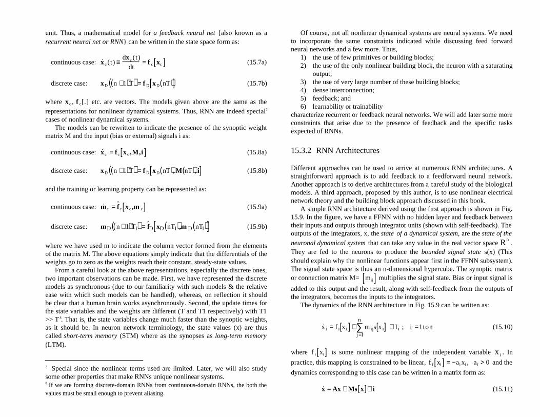
A simple RNN architecture derived using the first approach is shown in Fig.15.9. In the figure, we have a FFNN with no hidden layer and feedback betweentheir inputs and outputs through integrator units (shown with self-feedback). Theoutputs of the integrators, x, the state of a dynamical system, are the state of the

neuronal dynamical system that can take any value in the real vector space Rn.

They are fed to the neurons to produce the bounded signal state s(x) (Thisshould explain why the nonlinear functions appear first in the FFNN subsystem).The signal state space is thus an n-dimensional hypercube. The synoptic matrixor connection matrix M= mij[ ] multiplies the signal state. Bias or input signal is

added to this output and the result, along with self-feedback from the outputs ofthe integrators, becomes the inputs to the integrators.

The dynamics of the RNN architecture in Fig. 15.9 can be written as:

˙ x i = f i x i[ ] + m ijs x i[ ]j=1

n

∑ + I i ; i =1ton (15.10)

where f i xi[ ] is some nonlinear mapping of the independent variable x i . In

practice, this mapping is constrained to be linear, f i xi[ ] = −a i xi , a i > 0 and the

dynamics corresponding to this case can be written in a matrix form as:

˙ x = Ax + Ms x[ ]+ i (15.11)

where A is a diagonal matrix.

∑ ∑S[.]

S[.]

S[.]

x1

xN

Weigh&

sum

M.S[x]

∑

∑

Bias inputaddition

IN

I2

I1

∑ 1s

1s

+

+

+

+

Integration unitswith self-feedback

S(xN )

S(x1)f1[•]

f N[•]

˙ x 1

˙ x N

Figure 15-9. A continuous RNN architecture based on feedforward neural network andfeedback through integrator units.

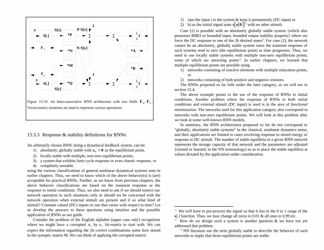
In the above model, all the signal states are assumed to be in a signal field Fxand used collectively to affect the future state. Such architecture is known asautoassociative or unidirectional. By adding another field Fy (with the

associated state y of size m) and allowing for cross connections as shown in Fig.15.10, we arrive at a dynamics given by:

˙ x ˙ y

=

A 0

0 B

x

y

+

P M

N Q

s x[ ]s y[ ]

+

i

j

(15.12)

Depending upon the characteristics of the synoptic sub-matrices P, M, N,and Q, we arrive at different network categories. When P = Q = [0], the resultingarchitecture is called hetro-associative. M = Nt leads to bi-directional networks(Fx feeding into the inputs of the integrators of field Fy and Fy feeding into

the inputs of the integrators of field Fx ). Here M is called the forward projection

or feedforward from neuron field Fx to the neuron field Fy and N backward or

feedback projection from neuron field Fy to neuron field Fx9. A special case of

bi-directional networks is the bi-directional associative memories or BAM(continuous additive bi-directional associative memory or CABAM since thedynamics is described in the continuous domain). In this architecture, the signalstates { s x[ ], s y[ ]} reach certain stable values given x 0[ ], y 0[ ] and hence

{ s x[ ], s y[ ]} can be considered as associative pairs.

When P and Q are not equal to zero, they are assumed to be symmetric (thisapplies to M of autoassociative architecture as well) with positive diagonalentries { pii , q ii > 0 }(excitory connections) and non-positive off-diagonal

elements { pij, q ij ≤ 0, i ≠ j } (inhibitory connections ). The symmetry is

considered to be a reflection of a lateral inhibition or a competitive connectiontopology10. The strength of the inhibitory connections is assumed to be adecreasing function of the distance i − j .

The inputs i i and jj , when present, are added directly to the dynamics in the

above models. Hence, such models are known as additive activation models . Wewill see other models as we study some well-known RNNs shortly. But let usfirst look at some central issues related to RNNs.

9 The readers may note that these classifications differ vastly from thedefinitions found in the classical network and system theory literature.10 We will discuss later the real requirement for symmetry using network interpretations.

15.3.3 Response & stability definitions for RNNs

An arbitrarily chosen RNN, being a dynamical feedback system, can be:1) absolutely, globally stable with x e = 0 as the equilibrium point,

2) locally stable with multiple, non-zero equilibrium points,3) a system that exhibits limit cycle response or even chaotic response, or4) completely unstable.

using the various classifications of general nonlinear dynamical systems seen inearlier chapters. Thus, we need to know which of the above behavior(s) is (are)acceptable for practical RNNs. Further, as we know from previous chapters, theabove behavior classifications are based on the transient response or theresponse to initial conditions. Thus, we also need to ask if we should restrict ournetwork operation to such situations only or should we be concerned with thenetwork operation when external stimuli are present and if so what kind ofstimuli? Constant valued (DC) inputs or one that varies with respect to time? Letus develop the answers to these questions using intuition and the possibleapplication of RNNs as our guide.

Consider the problem of the English alphabet (upper case only) recognitionwhere we might have a corrupted n r by n c bit-matrix to start with. We can

expect the information regarding the 26 correct combinations some how storedin the synoptic matrix M. We can think of applying the corrupted matrix:

1) a)as the input i to the system & keep it permanently (DC input) or2) b) as the initial signal state s x 0( )[ ]11 with no other stimuli.

Case (1) is possible with an absolutely globally stable system {which alsopossesses BIBO or bounded input, bounded output stability property} where weforce the DC response to one of the 26 desired states12. For case (2), the networkcannot be an absolutely, globally stable system since the transient response ofsuch systems tend to zero (the equilibrium point) as time progresses. Thus, weneed to use locally stable systems with multiple non-zero equilibrium points,some of which are attracting points13. In earlier chapters, we learned thatmultiple equilibrium points are possible using

1) networks consisting of reactive elements with multiple relaxation points,or

2) networks consisting of both positive and negative resistors.The RNNs proposed so far falls under the later category, as we will see in

section 15.4.The above example points to the use of the response of RNNs to initial

conditions. Another problem where the response of RNNs to both initialconditions and external stimuli (DC input) is used is in the area of functionalminimization. The networks used for this application category also correspond tonetworks with non-zero equilibrium points. We will look at this problem afterwe look at some well-known RNN models.

In summary, the RNN architectures proposed so far do not correspond to“globally, absolutely stable systems” in the classical, nonlinear dynamics sense,and their applications are limited to cases involving response to stored energy orresponse to DC stimuli. The number of stable equilibria in a given RNN networkrepresents the storage capacity of that network and the parameters are adjusted{trained or learned, in the NN terminology) so as to place the stable equilibria atvalues dictated by the application under consideration.

11 We will have to pre-process the signal so that it lies in the 0 to 1 range of thes[.] function. Thus, we may change all zeros to 0.01 & all ones to 0.99 etc.12 How do we design such a system is another question & we have not yetaddressed that problem.

13 NN literature use the term globally stable to describe the behavior of suchnetworks to imply that those equilibrium points are stable.

yJ

N S[y]

*M

S[x]1s

I

xI

P S[x]

S[.] *P ∑∑

1s

IS[y]

S[.] ∑∑

*N

*B

*A

Fy

Fx

*Q

Figure 15-10. An hetro-associative RNN architecture with two fields Fx , Fy .

Vector/matrix notations are used to represent various operations.

15.3.4 Some well known RNNs

15.3.4.1 Continuous Domain Models

15.3.4.1.1 Hopfield Model

A simple RNN model known as Hopfield circuit14 is given by:

c i˙ x i =−x iR i

+ m ijs j x j[ ]j=1

n

∑ + Ii ; i = 1ton (15.13)

where M = M t (symmetric synoptic matrix), s j x j[ ] > 0 , and monotonically

increasing, and bounded. That is, the Hopfield circuit corresponds to a specialcase of the autoassociative model seen before. This circuit, which re-ignited theinterest in NNs once again in the early 1980's, uses a synoptic matrix M that islearned (or computed) off-line and is shown to be useful in two applications:

1) cleaning up corrupted binary (or bipolar) data, and2) functional optimization.

In both the applications, the function s j x j[ ] > 0 is chosen to be the threshold

function (with output values of zero and one). In application #1, the corrupteddata is used as the initial value of the Signal State, s x[ ] , and the external stimuli

i is set equal to zero. After some iteration, the Signal State s x[ ] will settle to a

fixed value, providing the filtered data. Thus, as indicated earlier, the Hopfieldcircuits represent a locally stable system with multiple equilibrium points, one ofwhich is reached, depending upon the initial condition. In fact, it has beenshown that a specific M corresponds to making certain number of binary(bipolar) vectors as the attracting equilibrium points of the circuit and theresulting equilibrium point corresponding to an initial state is simply a storedvector with the least Hamming distance to the initial state15.

The coefficients c i , Ri , i i, m ij (i, j = 1 to n) of (15.13) represent the

degrees of freedom available in the Hopfield dynamics. By varying their valuesproperly, we can control the number of stable equilibria and their values. Wehave approximately n 2 (for n large) coefficients or degrees of freedom, whereaswe have 2 n possible signal state values. The growth in the number of degreesof freedom becomes very small compared to the possible signal state values asthe value of n increases. Therefore, we can expect the maximum number ofstable equilibria that is possible by the variation of these limited number of

14

15 Thus, there is also the possibility for oscillation as more than one stored vectorcan have the same, least Hamming distance to the initial state.

coefficients to be very small compared to the total number of signal states. It hasbeen shown through simulations and rigorous analytical approaches that themaximum number of stable equilibria or the storage capacity of Hopfieldnetwork is approximately equal to 0.15 × n, a very small number compared tothe total signal states of the dynamics. This can be considered a major limitationof Hopfield (and other RNN) dynamics, but we have to keep in mind that thelimited number of stable equilibria gives rise to better fault tolerance andgraceful degradation properties. Later we will consider if the storage capacitycan be increased through the use more complex nonlinear mapping functionsusing the network approach (section 15.3.4).

Tank and Hopfield recognized that their circuit could be used for a specialcase of functional optimization known as linear programming (LP). Given avariable vector x (x ∈Rn ), constant vectors a, c and constant matrix B, the taskin LP is to find the value of vector x such that the scalar cost function.

φ x[ ] = aTx (15.14)

is minimized and where the solution x satisfies the p constraints

f x[ ] = Bx − c ≥ 0 (15.15)

A simple example of this LP problem is the one-variable case (n = 1) with

φ x[ ] = x (15.16)

as the linear function to be minimized subject to a single constraint (p = 1)

f x[ ] = x ≥ 0 (15.17)

It can be noted that this simple problem has a unique solution given by x = 0.A first-order Hopfield circuit can be used to find the solution to this problem.The first-order dynamics is given by:

c ˙ x = −x

R+ m11s x[ ] + i (15.18)

Tank and Hopfield argued that the network minimizes a pseudo energyfunction16 E[x] given by: 16 Tank & Hopfield called this an energy function, similar to a Lyapunovfunction, as its time derivation evaluated along the circuit dynamics is negativesemi-definite. We have added the term pseudo to stress the possibility of thefunction E[x] becoming negative. Also, we will find later that the function thatreally gets minimized has the dimension of power and not energy. We discussed

E x[ ] = − i x +x 2

2R+ m11S v[ ]dv

0

x

∫ (15.19)

That is, the equilibrium point x e obtained from the dynamics of the Hopfield

circuit correspond to the minimum of E x[ ].

The circuit corresponding to the dynamics in (15.18) will provide thesolution to the LP problem if we can make the following identifications:

i = −1

m11 = 1

s x[ ] =o if x ≥ 0

−x if x < 0

(15.20)

leading to E x[ ] as:

E x[ ] = − x +x2

2R+ s v[ ]dv

0

x

∫ (15.21)

The first term in the above expression corresponds to the LP function to beminimized, and the other two terms are added to make the energy function largeras and when the constraint is not satisfied (a penalty function or constraint). Ifthe circuit is simulated with x(0) > 0, x(t) will tend to x e = 0 which is the

solution to the LP problem17.In summary, in this application we excite the network with an external DC

stimulus and some initial value and hope that the obtained solution isindependent of the initial condition. Of course, this is possible only if the errorfunction is bowl shaped with only one minimum. However, the dynamics andhence the cost function being minimized is in general nonlinear and hence theminimum reached may not be the global minimum.

this in general terms in chapter 3 and came across the term 'mixed potential'which is really getting minimized.

17 The choice of s[.] as given here will make x(t) → ∞ as t → ∞ for any

x(0) < 0. We will analyze the cause for this problem and look at an alternateenergy function as we study RNNs from 'Electrical Nets' perspective in section11.3.

15.3.4.1.2 Continuous Additive Bi-directional associative Memory(CABAM)

We have seen this model as we discussed the evolution of general RNNarchitectures from feedforward NNs. The dynamics is given by:

˙ x i = −a ix i + mijs j y j[ ]j=1

m

∑ + i i ; i = 1 to n

˙ y j = −ˆ a jy j + mijsi xi[ ]i=1

n

∑ + jj ; j =1 to m

(15.22)

It can be observed that this model is a hetro associative analog of theHopfield circuit. We will look at this model once again from an electricalnetwork perspective in section 15.4.

15.3.4.1.2.1 Grossberg Models

In this section, we present a number of biologically inspired RNN models toillustrate the slow and painful evolution leading to the various models.Restricting to an auto-associative model with field Fx of n neurons, Grossberg

models restrict the neuronal output to a finite range [0, Bi ] and hence are

mostly useful for pattern classification and recognition problems. A pattern isdenoted as p = [p1 p 2 L p n ]t where pi (i = 1 to n) are normalized such

that p ii=1

n∑ = 1 and thus pi can be considered as a probability distribution

corresponding to a pattern. Letting I(t) as the background illumination and I i (t)

the reflectance from the i-th element, we have I i = p iI with I ii=1

n

∑ = I and a

simple additive activation model can be written as:

˙ x i = −(a i + I i )x i + bi I i ; i = 1 to n (15.23)

The constant a i , which represents the term corresponding to self-feedback,

leads to a stable system, and has a decaying response when I i (t) = 0, is called

the passive decay rate. From the expression, we can note that x i is bounded in

the range [0, b i ]. Since in general I i (t) is a constant, this dynamics represent a

simple linear, uncoupled model whose solution can be written down easily.Since I i (t) affects only x i , the term additive activation . We can note that

x i → bi as I →∞ regardless of the value of pi . Grossberg calls this saturation

(an undesirable effect) of large inputs. He went on to suggest that the inputsI j ( j = 1to n, j ≠ i) should also be used in the expression for x i , in an

inhibitory sense. The corresponding simplest model is:

˙ x i = −(a i + I i )x i + a iI i − xi I jj≠ i∑

= −(a i + I)xi + a i I i

(15.24)

Thus, the dynamics represents an uncoupled, linear model for fixed I i (t)

and hence a closed form solution for x i (t) can be easily written. It can be shown

that x i (t) → p ib i as I →∞ . That is, we no longer have saturating outputs but

outputs that represent the pattern. Thus, the pattern information gets stored in theneuron outputs. Grossberg calls this multiplicative activation model..

The multiplicative model can be modified to allow the activation variablex i (t) to assume negative values in a finite range [ci , b i ], where c i > 0 and

c i << bi . This leads to what is known as a multiplicative, shunting activation

model::

˙ x i = −(a i + I)xi + b iI i − c i I jj≠i∑ (15.25)

A more general shunting activation is possible by allowing cross couplingbetween the various states x i (t) . Separating the inputs as excitory inputs I i and

inhibitory inputs J i , the model can be written as:

˙ x i = − a i + I i + J i( )x i + bi I i − c i Ji + c isi xi[ ]− c i s j x j[ ]j≠ i∑ − xi s i x i[ ] − sj x j[ ]

j≠ i∑

(15.26)

That is, for the first time in the evolution of the Grossberg models, we have atrue nonlinear model involving cross coupling between the various states, and ittook almost 15 years to get to this point. In the next section we will show howthese and other exotic RNN models that can be derived easily using the"building block concept" advanced in this book.

15.3.4.1.2.2 Cohen-Grossberg Model

A RNN model proposed by Cohen-Grossberg has the activation dynamics givenby:

˙ x i = −a i x i[ ] bi xi[ ] − m ijs j x j[ ]j=1

n

∑

(15.27)

where the function a i x i[ ] is assumed to be non-negative and bounded, s j •[ ]bounded monotone non-decreasing function, and b i xi[ ] belongs to the set that

ensures the stability of the activation dynamics.

15.3.4.1.2.3 Continuous Bi-directional Associative Memories

This model results from extension to hetro associative case of the above Cohen-Grossberg model and has the dynamics given by:

˙ x i = −a i x i[ ] b i x i[ ] − m ijs j y j[ ]j=1

m

∑

; i =1ton

˙ y j = −ˆ a j y j[ ] ˆ b j y j[ ] − mijˆ s i xi[ ]i=1

n

∑

; j = 1tom

(15.28)

where we have used ' ^ ' to differentiate the functions used for the Fx field

dynamics from those of Fy . In practice, all the nonlinear functions are made

identical to simplify the design problem.In summary, it can be noted that the RNN dynamics known so far

correspond to nonlinear dynamics that are not globally stable in the classicalsystem theory 18 sense. They correspond to dynamics with more than one locallystable equilibrium point that produce stable outputs under the application ofexternal, DC excitation. More importantly, they are carefully hand crafted tolead to the desired behavior.

15.3.4.2 Discrete RNN Models

Discrete RNN models often use neurons with threshold signal functions (binaryor bipolar output) and hence can be called bivalent RNN models. They can bederived:

1) by a direct approach that is, the dynamics will be represented bynonlinear difference equations, or

2) from an analog model and a suitable discretization procedure.we will use the later approach and present one specific model here. Consideringthe CABAM seen before (equation 15.22) and using the following substitutions:

a i , ˆ a j = 1T , ˆ m ij = T.m ij,

ˆ I i = T.I i , J i = T.Ji

d

dt= z −1

T

(15.29)

We obtain a discrete hetro associate dynamics as:

18 Another way to put it is to say that the electrical network architecturescorresponding to such dynamics are non-passive. We will use this line ofthinking in the next section.

xi k +1( ) = ˆ m ijs j y j k( )[ ]j=1

m

∑ + ˆ I i k( ) ; i =1to n

y j k +1( ) = ˆ m ijsi x i k( )[ ]i=1

n

∑ + ˆ J j k( ) ; j = 1tom

(15.30)

where k represents the time or iteration index. When ˆ I i (k), ˆ J i (k) are constant

(DC excitation), we expect x i (k), y i (k) to stabilize to some steady-state values

as k →∞ . When the neuron signal functions si •[ ], sj •[ ] are constrained to be

the threshold functions, the model reduces to the bi-directional associative orBAM model. The signal functions si •[ ], sj •[ ] can also be made complex while

retaining the threshold function property. For example:

si x i k + 1( )[ ] =1 if x i (k) > U i

si x i k( )[ ] if x i (k) = U i

0 if x i (k) < Ui

(15.31)

and similarly for s j •[ ] are used and where U i (V j for s j •[ ] ) is a threshold

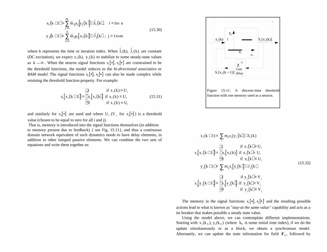
value (chosen to be equal to zero for all i and j). That is, memory is introduced into the signal functions themselves (in additionto memory present due to feedback) { see Fig. 15.11}, and thus a continuousdomain network equivalent of such dynamics needs to have delay elements, inaddition to other lumped passive elements. We can combine the two sets ofequations and write them together as:

x i (k + 1) = mijs j[y j k( )]j

∑ + I i (k)

s i x i k + 1( )[ ] =1 if x i k( ) > U i

si xi (k)[ ] if x i k( ) = Ui

0 if xi k( ) < U i

y j k + 1( ) = mijsi yi k( )[ ]i

∑ + J j k( )

s j y j k + 1( )[ ] =1 if y j k( ) > V j

s i y j k( )[ ] if y j k( ) = V j

0 if y j k( ) < V j

(15.32)

The memory in the signal functions si •[ ], sj •[ ] and the resulting possible

actions lead to what is known as "stay-at the same value" capability and acts as atie breaker that makes possible a steady state value.

Using the model above, we can contemplate different implementations.Starting with x i (k 0 ), yi (k 0 ) (where k0 is some initial time index), if we do the

update simultaneously or as a block, we obtain a synchronous model.Alternately, we can update the state information for field Fx , followed by

z−1

Unitdelay

xi(k)

xi

Si

u i

Si[x

i(k)]

Si[x i(k −1)]

1

Figure 15-11. A discrete-time thresholdfunction with one memory used as a neuron.

change in field Fy , again Fx , etc. or we can change one neuron at a time,

similar to a serial processing. (see Fig. 15.12 for a block diagrammaticrepresentation of these three cases). On one extreme, we can justify suchalternates by invoking precedence in biological neural systems. On the otherextreme, we can consider alternatives such as permutations and combinationsresulting from technological considerations. This is something to considerseriously.

15.3.5 Proof for RNN Stability --- NN Style

As indicated before, the term global stability, according to the NN literature,implies convergence to a stable (non-zero) state in response to initial conditionsand or DC inputs, which in different from the global, absolute stability definitionin the classical nonlinear dynamical systems sense. Now we will briefly studyhow researchers in the neural network area handle the proof of stability.

In NN literature, initially the stability (as defined above) proof has beenadvanced for discrete RNNs and extended later to continuous models. Thestability proof is patterned after the Lyapunov approach. It starts with theidentification of a quadratic function of the state variables, followed by a proofthat the function:

1) is bounded (both lower and upper) in magnitude,2) has a finite number of minimas, and3) the function evaluated along the system trajectory is a non-increasing

function of time.Thus, similar to the Lyapunov technique, it can be argued that the system

state reaches a value at which point the function has a minimum and remainthere forever. It should be recognized that unlike a Lyapunov function of aglobally or locally, absolutely stable system which represents the energy left inthat system (and hence always nonnegative), the quadratic functions of RNNscan become negative as well. We will now look at the quadratic functions fortwo specific RNNs.

15.3.5.1 Hopfield Network

The original, discrete Hopfield model is described by the following recursiveequation:

v i k + 1( ) = f i m ijv j k( )j

∑ + I i k( )

(15.33)

where

*M + I(Multiply by thematrix and addthe bias vector )

MI

n unitdelaysS[Y(k)]

I(k)S[X(k)]S[X(k +1)]X(k +1) S[*]

(n units ofFig. 15.11)

*M t + JMultiply by thematrix and addthe bias vector )

M t

J

m unitdelays S[Y(k)]

S[X(k)]

J(k)

Y(k +1) S[Y(k +1)]S[*](m units ofFig. 15.11)

-1/32

(b) A two-phase clock

S[*](element ofFig. 15.11)

S[*](element ofFig. 15.11)

Unitdelayelement

Unitdelayelement

mutiply bythe wtsand add bias

m1j

mutiply bythe wtsand add bias

m i1

m+n phase clock

J1(k)

y1(k +1)

I1(k)

x1(k +1)S[x1 (k +1)]

S[y1 (k +1) S[y1 (k)]]S[X(k) ]

other S[y j(k) ]

S[x1 (k)]calculation of y1(k +1), S[y1]

calculation of x1(k +1), S[x1]

(c)

Clock for syncrhronization(a)

*M t + JMultiply by thematrix and addthe bias vector )

M t

J

m unitdelays

S[Y(k)]S[X(k)]

J(k)

S[Y(k +1)]Y(k +1) S[*](m units ofFig. 15.11)

*M + I(Multiply by thematrix and addthe bias vector )

MI

n unitdelays

S[Y(k)]

I(k)

S[X(k)]S[X(k +1)]X(k +1) S[*](n units ofFig. 15.11)

Figure 15-12. Different implementation schemes for RNNs: a) Synchronous model;b) Semi-synchronous; c) Serial. The functions of the various blocks can be seenfrom equation (15.32).

f i x[ ] =1 when x ≥ U i

0 when x < U i

(15.34)

with U i representing the threshold values and m ij = m ji and mii = 0. The

pseudo energy function associated with this dynamics is:

E = −1

2mijv iv j

j≠ i∑

i∑ − I ivi

i∑ + v i

2

i∑ (15.35)

which can be shown to be bounded from below and above. The change ∆E in Edue to the change in the state of neuron v i by ∆vi is:

∆E = − m ijv jj≠i∑ + I i − vi

∆v i (15.36)

which can be seen to be always negative. Since E is bounded, the recursion thusleads to stable states that do not further change with time.

The continuous version of this model is given by:

c i

dui

dt= m ijv j u j[ ]

j≠ i∑ −

u i

R i

+ I i (15.37)

where c i , Ri are positive constants, m ij = m ji and mii = 0 and v i •[ ] is chosen

to be a continuous and monotone increasing function of the input u i such as a

sigmoid function s •[ ]. The pseudo energy function19 E associated with this

dynamics is:

E = − m ijviv jj

∑i

∑ +1

R i

si−1 v i[ ]dv i

0

vi

∫i

∑ + I ivii

∑ (15.38)

The time derivative of E evaluated as the system trajectory is:

dE

dt= − c i

d(Si−1 [v i ])

dti∑ dvi

dt

2

≤ 0

(15.39)

for a monotone increasing function si[.] . Thus, the dynamics reach a stable

state at which E is minimum. 19 The function is no longer quadratic in the state variables.

15.3.5.2 Discrete Bivalent BAM Model

We have seen this discrete model before (equation 15.30). The quadraticfunction associated with this model is given by (using vector notations):

E = −s x[ ]Ms y[ ] − s x[ ] I − U[ ] t − s y[ ] J − v[ ]t(15.40)

where again it can be shown that E is bounded in magnitude and decreases alongthe system trajectory indicating the stability of the steady state value.

In summary, a quadratic or a suitable function of the state variables is used toprove stability of the states in the presence of external DC stimuli. The functionsseem to have resulted from intuition and experience. In fact, the followingparagraph from a book by Bart Kosko summarizes the existing situation:

"Monotonicity of a Lyapunov function provides a sufficient notnecessary condition for stability and asymptotic stability. Inability toproduce a Lyapunov function proves nothing. The system may or maynot be stable. Demonstration of a Lyapunov function, any Lyapunovfunction, proves stability. Unfortunately, other than a quadratic guess,in general we have no constructive procedure for generating Lyapunovfunctions"

The above statements highlight the limitations of the Lyapunov test itself{and we have learned these limitations in chapter 2 on general nonlinearsystems} and the difficulty in generating the Lyapunov function for an arbitrarydynamics. In the next section, we will see how a network theory approach canbe used to systematically obtain various RNN models and the Lyapunovfunctions associated with such nets.

15.4 RNNs Using Passive and Active Electrical NetBuilding Blocks

15.4.1 General Concept

In this section, we consider deriving new RNN architectures and the associatednonlinear dynamics using electrical network building blocks. We will also showhow the existing models can be considered as special cases of architecturesresulting from the building block approach. We will first take another look at theresponses that result from the use of various building blocks (passive and active)with varying characteristics and use that information to define the necessarycharacteristics of building block for RNNs.

The different possibilities for building nonlinear nets using nonlinearbuilding blocks are shown in Fig. 15.13. As a minimum, we can form nonlinear

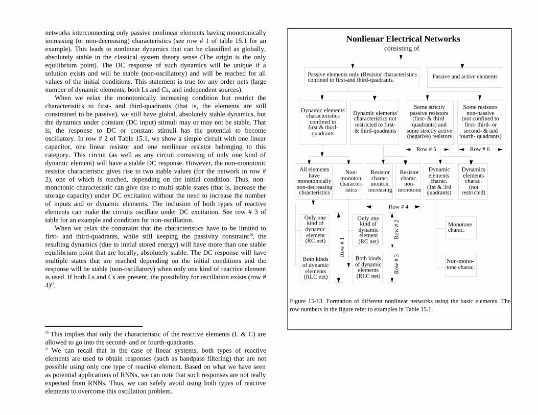
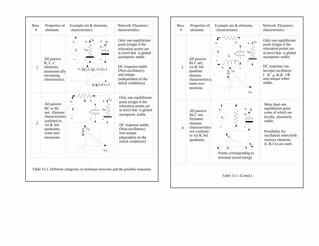
networks interconnecting only passive nonlinear elements having monotonicallyincreasing (or non-decreasing) characteristics (see row # 1 of table 15.1 for anexample). This leads to nonlinear dynamics that can be classified as globally,absolutely stable in the classical system theory sense (The origin is the onlyequilibrium point). The DC response of such dynamics will be unique if asolution exists and will be stable (non-oscillatory) and will be reached for allvalues of the initial conditions. This statement is true for any order nets (largenumber of dynamic elements, both Ls and Cs, and independent sources).

When we relax the monotonically increasing condition but restrict thecharacteristics to first- and third-quadrants (that is, the elements are stillconstrained to be passive), we still have global, absolutely stable dynamics, butthe dynamics under constant (DC input) stimuli may or may not be stable. Thatis, the response to DC or constant stimuli has the potential to becomeoscillatory. In row # 2 of Table 15.1, we show a simple circuit with one linearcapacitor, one linear resistor and one nonlinear resistor belonging to thiscategory. This circuit (as well as any circuit consisting of only one kind ofdynamic element) will have a stable DC response. However, the non-monotonicresistor characteristic gives rise to two stable values (for the network in row #2), one of which is reached, depending on the initial condition. Thus, non-monotonic characteristic can give rise to multi-stable-states (that is, increase thestorage capacity) under DC excitation without the need to increase the numberof inputs and or dynamic elements. The inclusion of both types of reactiveelements can make the circuits oscillate under DC excitation. See row # 3 oftable for an example and condition for non-oscillation.

When we relax the constraint that the characteristics have to be limited tofirst- and third-quadrants, while still keeping the passivity constraint 20, theresulting dynamics (due to initial stored energy) will have more than one stableequilibrium point that are locally, absolutely stable. The DC response will havemultiple states that are reached depending on the initial conditions and theresponse will be stable (non-oscillatory) when only one kind of reactive elementis used. If both Ls and Cs are present, the possibility for oscillation exists (row #4)21.

20 This implies that only the characteristic of the reactive elements (L & C) areallowed to go into the second- and or fourth-quadrants.21 We can recall that in the case of linear systems, both types of reactiveelements are used to obtain responses (such as bandpass filtering) that are notpossible using only one type of reactive element. Based on what we have seenas potential applications of RNNs, we can note that such responses are not reallyexpected from RNNs. Thus, we can safely avoid using both types of reactiveelements to overcome this oscillation problem.

Passive and active elementsPassive elements only (Resistor characteristicsconfined to first-and third-quadrants.

Some strictlypassive resistors(first- & third quadrants) and

some strictly active(negative) resistors

Dynamic elements'characteristics notrestricted to first-& third-quadrants

Some resistorsnon-passive

(not confined tofirst- third- orsecond- & and

fourth- quadrants)

Dynamic elements'characteristics

confined tofirst & third-

quadrants

Row # 5 Row # 6

Nonlienar Electrical Networksconsisting of

Non-monoton.character-

istics

All elementshave

monotonicallynon-decreasingchracteristics

Resistorcharac.

non-monotone

Resistorcharac.monton.

increasing

Dynamicelementscharac.

(1st & 3rdquadrants)

Dynamicselementscharac.

(notrestricted)

Row # 4

Non-mono-tone charac.

Monotonecharac.

Both kindsof dynamic

elements(RLC net)

Only onekind of

dynamicelement(RC net)

Both kindsof dynamic

elements(RLC net)

Only onekind of

dynamicelement(RC net)

Row

# 1

Row

# 3

Row

# 2

Figure 15-13. Formation of different nonlinear networks using the basic elements. Therow numbers in the figure refer to examples in Table 15.1.

Row #

Properties ofelements

Example net & elements, characteristics.

Network /Dynamicscharacteristics

˙ q v c

+

-

+

-

Is

+

-

v R

iR

All passiveR, L, C elements;monotonicallyincreasingchracteristics.

Only one equilibriumpoint (origin if therelaxation points areat zero) that is globalasymptotic stable.

DC response stable(Non-oscillatory)and unique(independent of theinitial conditions)

+

-

E

+

-

vR

i R+

-

c

R

1

2

All passiveRC or RLnet; Elementcharacteristicsconfined to 1st & 3rdquadrants;some non-monotone.

q,φ ,i R (v R )

v c [q], iL [φ], vR (iR )

v R

i RER

Only one equilibriumpoint (origin if therelaxation points areat zero) that is globalasymptotic stable.

DC response stable,(Non-oscillatory)non-unique(dependent on theinitial conditions)

Table 15-1. Different categories of nonlinear networks and the possible responses.

+

-

E

+

-

vR

i R+

-

c

+ -

L

˙ q v c

+

-

+

-

Is

Row #

Properties ofelements

Example net & elements, characteristics.

Network /Dynamicscharacteristics

All passiveRLC net;1st & 3rdquadrantelementcharacteristics;some non-montone.

Only one equilibriumpoint (origin if therelaxation points areat zero) that is globalasymptotic stable.

3

All passiveRLC net;Dynamicelementcharacteristicsnot confinedto 1st & 3rdquadrants.

More than oneequilibrium pointsome of which arelocally, absolutelystable.

Possibility foroscillation when bothreactive elements(L & Cs) are used.

v R

i RE

R

q c

v c

Points corresponding tominimal stored energy

4

DC response canbecome oscillatory( ) &non-unique whenstable.

R2

≤ 4L c

Table 15-1. (Contd.)

We can form nonlinear networks not only with passive elements, but activeelements, especially negative resistors, if some precautions are taken. First andforemost, we need to make certain that the combined maximum powergeneration capacity p gmax (t)( ) of the negative resistors do not exceed the

combined power absorption capacity pamax (t)( ) of the positive resistors. This

restriction will ensure that the state values remain in a finite range and notbecome infinite. The requirement that pgmax(t) < pamax(t) can be accomplished

either by:1) by choosing the resistive element characteristic properly, and or2) limiting the maximum voltage across (or current through) the negative

resistors though proper choice of the reactive elements' characteristics.We also need to make pamax(t) < pgmax(t) when the system state is close to

origin so that the origin does not become a stable equilibrium point.A simple example of the first case is shown in row # 5 of the table where we

have a net with a linear capacitor (C = 1), a linear, negative resistor (resistance =-R) and a passive, nonlinear resistor with a current Vs voltage characteristicsgiven by:

i R vR[ ] = k1 tan k 2vR[ ] ; k1 , k 2 > 0 (15.41)

It can be noted that for vR (= vR1 = v r2 = v c ) > 1k2 in magnitude, the power

absorbed by the nonlinear, passive resistor pa (t) = k1 tan k 2v c (t)[ ]v c (t){ } is

much greater than the power generated by the linear, negative resistorpg (t) = v c

2 R{ } . We can also arrive at the same conclusion by looking at the

combined v-i characteristic of the two resistors in parallel as shown in the table.The characteristics indicate a negative resistance function for small values of theindependent variable v c (t) and a positive resistance for higher values of v c (t) .

The value of v c (t) ≠ 0 at which the current equals zero becomes the equilibrium

point of the dynamics of this network.An example of the second case is also shown in the table (row # 6). In this

network, the capacitor is made nonlinear, with a v-q characteristic given by,

v c q c[ ] =

2

πtan−1 q c[ ] , (15.42)

the negative resistor is made linear, and the passive resistor is made nonlinearwith a v-i characteristic given by:

i R[vR ] = k1 tanπ2

vR

(15.43)

+

-

c

+

-

i R2v R2

v R1

i R1+

-

+

-

+

-

i R2v R2

v R1

i R1

+

-

i R1 v R1[ ]

i R2 v R2[ ]

i R1 v R1[ ]

i R2 v R2[ ]

q c

v c

Row #

Properties ofelements

Example net & elements, characteristics.

Network /Dynamicscharacteristics

Passive/ActiveRC or RL net;Reactiveelementslinear; somenegative &positive Rs(nonlinear).

Stable nonzero valuedequilibrium points. Nooscillation when onlyone type of reactiveelements are used.

5

6

Passive/ActiveRC or RL net;Reactiveelementsnonlinear;some negative& positive Rs(nonlinear).

Stable nonzero valuedequilibrium points. Nooscillation when onlyone type of reactiveelements are used.

Table 15-1. (Contd.)

Again, we achieve the descried effect pgmax(t) < pamax(t) as v c (t) →1

For both networks, origin, which is another equilibrium point, is not a stableone. Some other value of v c (t) ≠ 0 at which pg (t) = pa (t) becomes the stable

equilibrium point. Thus, in a true sense, there is no energy function that getsdepleted but we have the situation of power balance at these equilibrium points.We will also find the DC response of these two networks to be stable as thenetwork has only one type of reactive element.

As in the case of passive nonlinear nets, we can relax the condition that theelement characteristics be monotonically increasing and arrive at similarconclusions such as increased storage capacity etc.

In summary, based on what we have seen in the last section (that RNNsneeds to have non-zero equilibrium states) and the above discussions, we canexpect that numerous RNN architectures and their associated dynamics can beobtained from properly connected nonlinear nets consisting of positive,negative, and non-passive resistors. Further, to avoid oscillations under DCstimuli, we will assume that only networks with only one kind of reactiveelement will be used to arrive at such RNN architectures. We now provide thedetails for one general architecture and discuss its dynamics.

15.4.2 Specific RNN Architectures

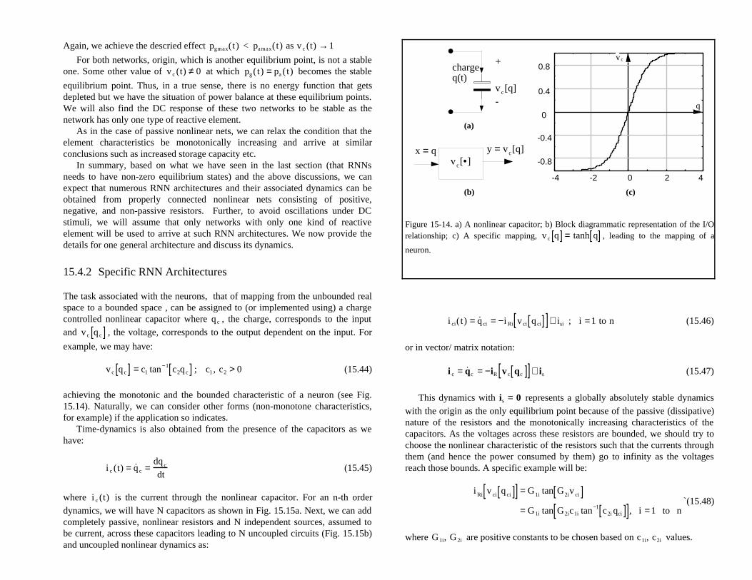
The task associated with the neurons, that of mapping from the unbounded realspace to a bounded space , can be assigned to (or implemented using) a chargecontrolled nonlinear capacitor where q c , the charge, corresponds to the input

and v c q c[ ] , the voltage, corresponds to the output dependent on the input. For

example, we may have:

v c q c[ ] = c1 tan−1 c2q c[ ] ; c1 , c2 > 0 (15.44)

achieving the monotonic and the bounded characteristic of a neuron (see Fig.15.14). Naturally, we can consider other forms (non-monotone characteristics,for example) if the application so indicates.

Time-dynamics is also obtained from the presence of the capacitors as wehave:

i c (t) = ˙ q c =dq c

dt(15.45)

where i c (t) is the current through the nonlinear capacitor. For an n-th order

dynamics, we will have N capacitors as shown in Fig. 15.15a. Next, we can addcompletely passive, nonlinear resistors and N independent sources, assumed tobe current, across these capacitors leading to N uncoupled circuits (Fig. 15.15b)and uncoupled nonlinear dynamics as:

i ci(t) = ˙ q ci = −i Ri v ci q ci[ ][ ]+ isi ; i = 1 to n (15.46)

or in vector/ matrix notation:

i c = ˙ q c = −iR v c qc[ ][ ]+ is (15.47)

This dynamics with is = 0 represents a globally absolutely stable dynamics

with the origin as the only equilibrium point because of the passive (dissipative)nature of the resistors and the monotonically increasing characteristics of thecapacitors. As the voltages across these resistors are bounded, we should try tochoose the nonlinear characteristic of the resistors such that the currents throughthem (and hence the power consumed by them) go to infinity as the voltagesreach those bounds. A specific example will be:

i Ri v ci q ci[ ][ ] = G1i tan G2iv ci[ ]= G1i tan G2ic1i tan−1 c2i qci[ ][ ], i = 1 to n

`(15.48)

where G1i, G2i are positive constants to be chosen based on c1i, c2i values.

-4 -2 0 2 4

-0.8

-0.4

0

0.4

0.8

(a)

v c[q]

+

-

chargeq(t)

x = q y = v c[q]v c[•]

(b) (c)

q

v c

Figure 15-14. a) A nonlinear capacitor; b) Block diagrammatic representation of the I/Orelationship; c) A specific mapping, v c q[ ] = tanh q[ ] , leading to the mapping of a

neuron.

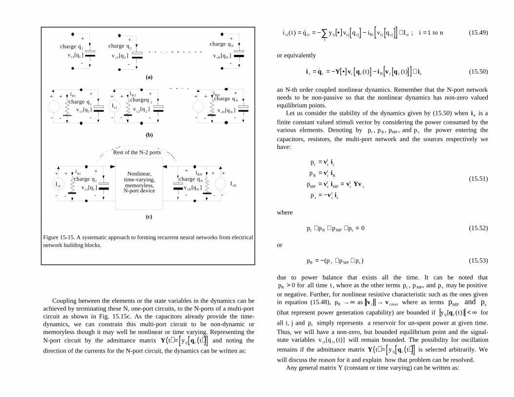
Coupling between the elements or the state variables in the dynamics can beachieved by terminating these N, one-port circuits, to the N-ports of a multi-portcircuit as shown in Fig. 15.15c. As the capacitors already provide the time-dynamics, we can constrain this multi-port circuit to be non-dynamic ormemoryless though it may well be nonlinear or time varying. Representing theN-port circuit by the admittance matrix Y t( ) = y ij qc t( )[ ][ ] and noting the

direction of the currents for the N-port circuit, the dynamics can be written as:

i ci(t) = ˙ q ci = − y ij •[ ]vcj q cj[ ]j

∑ − iRi vcj q cj[ ][ ] + Isi ; i = 1 to n (15.49)

or equivalently

i c = ˙ q c = −Y •[ ]vc qc (t)[ ] − i R v c q c (t)[ ][ ]+ is (15.50)

an N-th order coupled nonlinear dynamics. Remember that the N-port networkneeds to be non-passive so that the nonlinear dynamics has non-zero valuedequilibrium points.

Let us consider the stability of the dynamics given by (15.50) when i s is a

finite constant valued stimuli vector by considering the power consumed by thevarious elements. Denoting by pc , pR , pMP , and p s the power entering the

capacitors, resistors, the multi-port network and the sources respectively wehave:

pc = vct ic

pR = vct iR

pMP = vct iMP = vc

t Yv c

p s = −v ct is

(15.51)

where

pc + pR + pMP + ps = 0 (15.52)

or

pR = −(p c + pMP + ps ) (15.53)

due to power balance that exists all the time. It can be noted thatpR > 0 for all time t , where as the other terms pc , pMP, and p s may be positive

or negative. Further, for nonlinear resistive characteristic such as the ones givenin equation (15.48), pR →∞ as v c → v cmax where as terms pMP and ps

(that represent power generation capability) are bounded if y ij[qc (t)] < ∞ for

all i, j and pc simply represents a reservoir for un-spent power at given time.

Thus, we will have a non-zero, but bounded equilibrium point and the signal-state variables v ci[q ci (t)] will remain bounded. The possibility for oscillation

remains if the admittance matrix Y t( ) = y ij qc t( )[ ][ ] is selected arbitrarily. We

will discuss the reason for it and explain how that problem can be resolved.Any general matrix Y (constant or time varying) can be written as:

+

-

charge q1

v c1[q1 ]

+

-

charge q2

v c2[q2 ]

+

-

charge qN

v cN[qN ]

(a)

+

-

charge qN

v cN[qN ]

iRN

I sNIs1

iR1 +

-

+

-

iR2

I s2

(b)

+

-

charge q1

v c1[q1 ]

+

-

+

-

+

-

chargeq2

vc2

[q2]

+

-

+

-

+

-

charge q1

v c1[q1 ]

+

-

+

-

I s1

iR1

charge qN

v cN[qN ]

iRN +

-

+

-

I sN

+

-

Nonlinear,time-varying,memoryless,

N-port device

(c)

Rest of the N-2 ports

Figure 15-15. A systematic approach to forming recurrent neural networks from electricalnetwork building blocks.

Y = Y s + Ya (15.54)

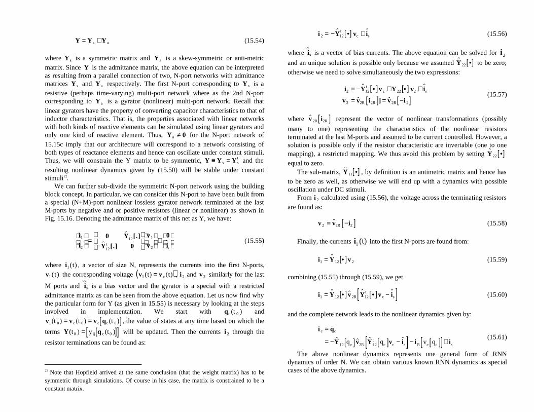
where Y s is a symmetric matrix and Ya is a skew-symmetric or anti-metric

matrix. Since Y is the admittance matrix, the above equation can be interpretedas resulting from a parallel connection of two, N-port networks with admittancematrices Y s and Ya respectively. The first N-port corresponding to Y s is a

resistive (perhaps time-varying) multi-port network where as the 2nd N-portcorresponding to Ya is a gyrator (nonlinear) multi-port network. Recall that

linear gyrators have the property of converting capacitor characteristics to that ofinductor characteristics. That is, the properties associated with linear networkswith both kinds of reactive elements can be simulated using linear gyrators andonly one kind of reactive element. Thus, Ya ≠ 0 for the N-port network of

15.15c imply that our architecture will correspond to a network consisting ofboth types of reactance elements and hence can oscillate under constant stimuli.Thus, we will constrain the Y matrix to be symmetric, Y ≡ Y s = Y s

t and the

resulting nonlinear dynamics given by (15.50) will be stable under constantstimuli22.

We can further sub-divide the symmetric N-port network using the buildingblock concept. In particular, we can consider this N-port to have been built froma special (N+M)-port nonlinear lossless gyrator network terminated at the lastM-ports by negative and or positive resistors (linear or nonlinear) as shown inFig. 15.16. Denoting the admittance matrix of this net as Y, we have:

i1

i2

=

0 ˆ Y 12 [.]

− ˆ Y 12t [.] 0

v 1

v 2

+

0ˆ i s

(15.55)

where i1 (t) , a vector of size N, represents the currents into the first N-ports,

v1 (t) the corresponding voltage v1 (t) = v c (t)( ), i 2 and v 2 similarly for the last

M ports and ˆ i s is a bias vector and the gyrator is a special with a restricted

admittance matrix as can be seen from the above equation. Let us now find whythe particular form for Y (as given in 15.55) is necessary by looking at the stepsinvolved in implementation. We start with qc (t 0 ) and

v1 (t 0 ) = v c (t 0 ) = v c qc (t 0 )[ ], the value of states at any time based on which the

terms Y(t0 ) = y ij q c (t0 )[ ][ ] will be updated. Then the currents i 2 through the

resistor terminations can be found as:

22 Note that Hopfield arrived at the same conclusion (that the weight matrix) has to besymmetric through simulations. Of course in his case, the matrix is constrained to be aconstant matrix.

i 2 = − ˆ Y 12t •[ ] vc + ˆ i s (15.56)

where ˆ i s is a vector of bias currents. The above equation can be solved for i2

and an unique solution is possible only because we assumed ˆ Y 22 •[ ] to be zero;

otherwise we need to solve simultaneously the two expressions:

i2 = − ˆ Y 12t •[ ]v c + Y22 •[ ] v2 + ˆ i s

v 2 = ˆ v 2R i2R[ ]] = ˆ v 2R −i 2[ ](15.57)

where ˆ v 2R i2R[ ] represent the vector of nonlinear transformations (possibly

many to one) representing the characteristics of the nonlinear resistorsterminated at the last M-ports and assumed to be current controlled. However, asolution is possible only if the resistor characteristic are invertable (one to onemapping), a restricted mapping. We thus avoid this problem by setting ˆ Y 22 •[ ]equal to zero.

The sub-matrix, ˆ Y 11 •[ ] , by definition is an antimetric matrix and hence has

to be zero as well, as otherwise we will end up with a dynamics with possibleoscillation under DC stimuli.

From i 2 calculated using (15.56), the voltage across the terminating resistors

are found as:

v 2 = ˆ v 2R −i2[ ] (15.58)

Finally, the currents i1 (t) into the first N-ports are found from:

i1 = ˆ Y 12 •[ ]v 2 (15.59)

combining (15.55) through (15.59), we get

i1 = ˆ Y 12 •[ ] ˆ v 2Rˆ Y 12

t •[ ]v c − ˆ i s[ ] (15.60)

and the complete network leads to the nonlinear dynamics given by:

i c = ˙ q c

= − ˆ Y 12 q c[ ] ˆ v 2Rˆ Y 12

t qc[ ]vc − ˆ i s[ ] − i R vc qc[ ][ ]+ is

(15.61)

The above nonlinear dynamics represents one general form of RNNdynamics of order N. We can obtain various known RNN dynamics as specialcases of the above dynamics.

15.4.2.1 Continuous BAM Dynamics from Network Dynamics

we can arrive at the continuous BAM dynamics. by restricting the terminationresistances at the M-ports to be linear resistors, the admittance matrix Y of the

multi-port to be a constant matrix, the bias vector ˆ i s to be zero, the v c Vs q

characteristics to be a sigmoidal functions and the characteristics of the resistorsin parallel with the capacitors to be inverse sigmoidal functions, Under theseconstraints, we get:

v c[qc ] = tanh[qc ]

iR [vc ] = G tanh−1 [v c ] = Gqc

ˆ i s = 0

ˆ v 2R[ˆ i R] = − ˆ R ̂ i R

(15.62)

where G is a N × N diagonal matrix with positive elements and ˆ R is a M × M

diagonal matrix with real coefficients. At least one of the elements of ˆ R has tobe negative to make the ( N + M( ) -port network and hence the total network

non-passive. The RNN dynamics in (15.61), reduces to

˙ q c = ic

= − ˆ Y 12ˆ R ˆ Y 12

t v c qc[ ]− ˆ i s( ) − iR v c qc[ ][ ] + is

= −Yvc q c[ ] − Gqc + i s

(15.63)

where Y is a symmetric, constant matrix. It is known that any constant,symmetric matrix Y can be obtained from:

Y = ˆ Y 12ˆ R ˆ Y 12

t (15.64)

by choosing M to be at least equal to N. Thus, the architecture in Fig. 15.15with the restrictions as given in (15.62) leads to the continuous form of Hopfielddynamics23.

23 Readers familiar with the performance of discrete-domain Hopfield networks may notethat the dynamics from such networks are prone to oscillation, whereas here we claimthat the dynamics will not oscillate as we have only one kind of reactive element. Thethreshold type (discontinuous) nonlinearities used in discrete models are the reason forthe oscillation and there will not be any oscillation if they are replaced by sigmoidalnonlinearities..

15.4.3 Function being minimized by Nonlinear Dynamics fromRecurrent Neural Networks

From the above discussions, it should be clear that the electrical networkequivalent of dynamics corresponding to RNNs consists of at least one negativeresistor and may also have constant forcing functions as inputs. The negativeresistors and the constant valued excitations inject power into the network andthe passive resistors consume power on a continuos basis. When a stableconstant equilibrium is reached, there is a simply a power balance between thesource elements and the sinks. Thus, what we have is not a situation of energybeing minimized (or the dynamics reaching a state corresponding to the minimaof an energy function) but a situation where a power balance (between sourcesand sinks) is reached and power is supplied by the sources to the sinkscontinuously. In section 3.3, we discussed a function known as mixed potentialhaving the dimension of power that can be formulated and whose minima (withrespect to the state variables) point to the equilibrium points. Further details canbe found in that section.

15.4.4 Storage Capacity of New RNN Architectures

Use a simple first- or second-order network with complex capacitor and resistorcharacteristics to show that many equilibrium points can be obtained and one ofwhich is reached depending upon the initial conditions.

15.4.5 Training based on Network Concepts

Use simulations performed by Zamarreno, visiting scholar from Spain

15.5 Summary