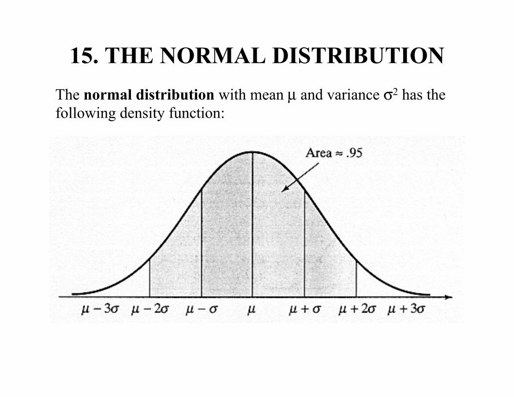
15. THE NORMAL DISTRIBUTIONThe normal distribution with mean µ and variance σ2 has the following density function:

The normal distribution is sometimes called a GaussianDistribution, after its inventor, C.F. Gauss (1777-1855).

The mathematical formula for the normal f (x) is given in Sincich, p. 257. We won't be needing this formula; just tables of areas under the curve.

• f (x) has a bell shape, is symmetrical about µ, and reaches itsmaximum at µ.

• µ and σ determine the center and spread of the distribution.

• The empirical rule holds for all normal distributions:68% of the area under the curve lies between (µ − σ, µ + σ)95% of the area under the curve lies between (µ − 2σ, µ + 2σ)99.7% of the area under the curve lies between (µ − 3σ, µ + 3σ)

• The inflection points of f (x) are at µ − σ, µ + σ . This helps us to draw the curve. It also allows us to visualize σas a measure of spread in the normal distribution.

• f (x) extends indefinitely in both directions, but almost allof the area under f (x) lies within 4 standard deviations from the mean (µ − 4σ, µ + 4σ). Thus, outliers more than 4 standard deviations from the mean will be extremely rare if the population distribution is normal.

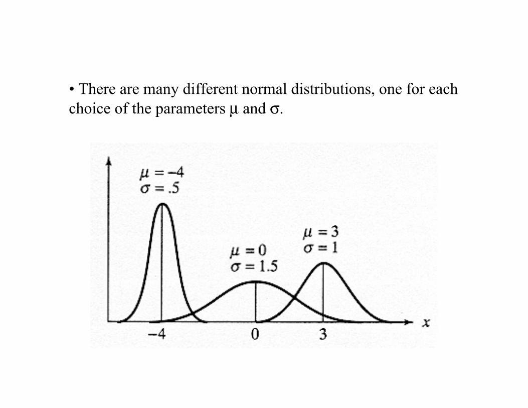
• There are many different normal distributions, one for eachchoice of the parameters µ and σ.

The normal distribution plays an extremely important role in statistics because

1) It is easy to work with mathematically

2) Many things in the world have nearly normal distributions:

Heights of ocean waves (but not Tsunamis!)IQ scores (by design).Stock Returns, according to Black-Scholes Theory.Weights of “4 ounce” bags of M&Ms.The high temperature in Central Park on January 1.The distance from the darts to the bulls-eye on a dartboard.The price of gold one month from now, assuming no big change in volatility.

3) The normal distribution is used in value at risk (VAR) calculations. VAR is a statistical risk measure used extensivelyfor measuring the market risk of portfolios of assets and/or liabilities. See website athttp://www.contingencyanalysis.com/glossaryvalueatrisk.htm

4) Sample means tend to have normal distributions, even if therandom variables being averaged do not. This amazing fact provides the foundation for statistical inference, and therefore for many of the things we will do in this course.

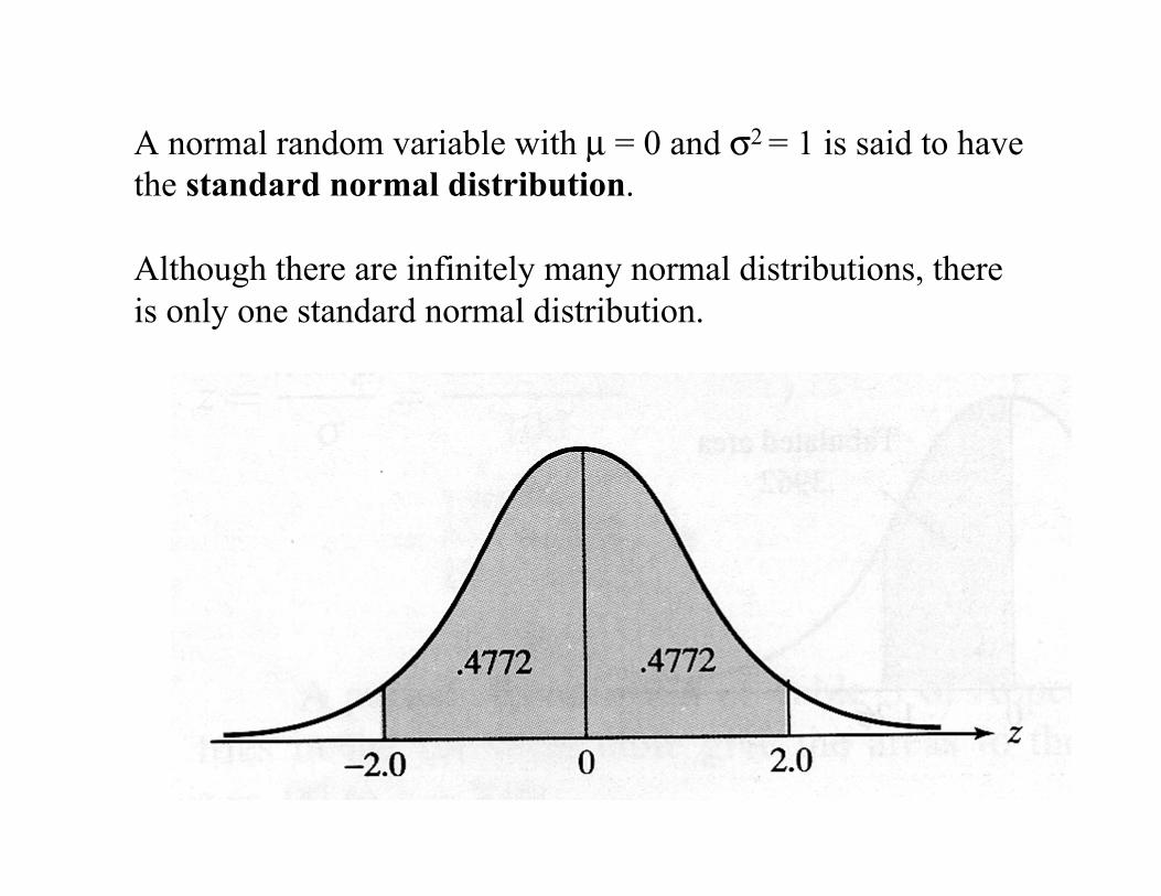
A normal random variable with µ = 0 and σ2 = 1 is said to have the standard normal distribution.

Although there are infinitely many normal distributions, there is only one standard normal distribution.

All normal distributions are bell-shaped, but the bell for the standard normal distribution has been standardized so that its center is at zero, and its spread (the distance from the center to the inflection points) is 1. This is the same standardization used in computing z-scores, so we will often denote a standard normal random variable by Z. We will use φ(z) to denote the density function for a standard normal.

To calculate probabilities for standard normal random variables, we need areas under the curve φ(z). These are tabulated in Table IV of Appendix B.

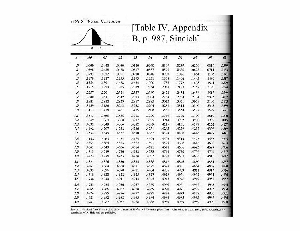
[Table IV, Appendix B, p. 987, Sincich]

To avoid confusion, replace z in Table IV by z0. In the diagram, change z to z0, and then label the horizontal axis as the z-axis.

Table IV gives the areas under φ(z) between z = 0 and z = z0.This is the probability that a standard normal random variablewill take on a value between 0 and z0.

For example, the probability that a standard normal is between 0and 2 is 0.4772.

The table includes only positive values z0.To get areas for more general intervals, use the symmetry property, and the fact that the total area under φ(z) must be 1.

Eg: If Z is standard normal, compute P(−1 ≤ Z ≤ 1), P(−2 ≤ Z ≤ 2) and P(−3 ≤ Z ≤ 3).

Solution: P(−1 ≤ Z ≤ 1) = 2(0.3413) = 0.6826P(−2 ≤ Z ≤ 2) = 2(0.4772) = 0.9544P(−3 ≤ Z ≤ 3) = 2(0.4987) = 0.9974.

Note: This shows that the empirical rule holds for standardnormal distributions. We still need to prove it for general normal distributions.

Eg: Compute the probability that a standard normal RV will be a) Between 1 and 3b) Greater than −0.47c) Less than −1.35.

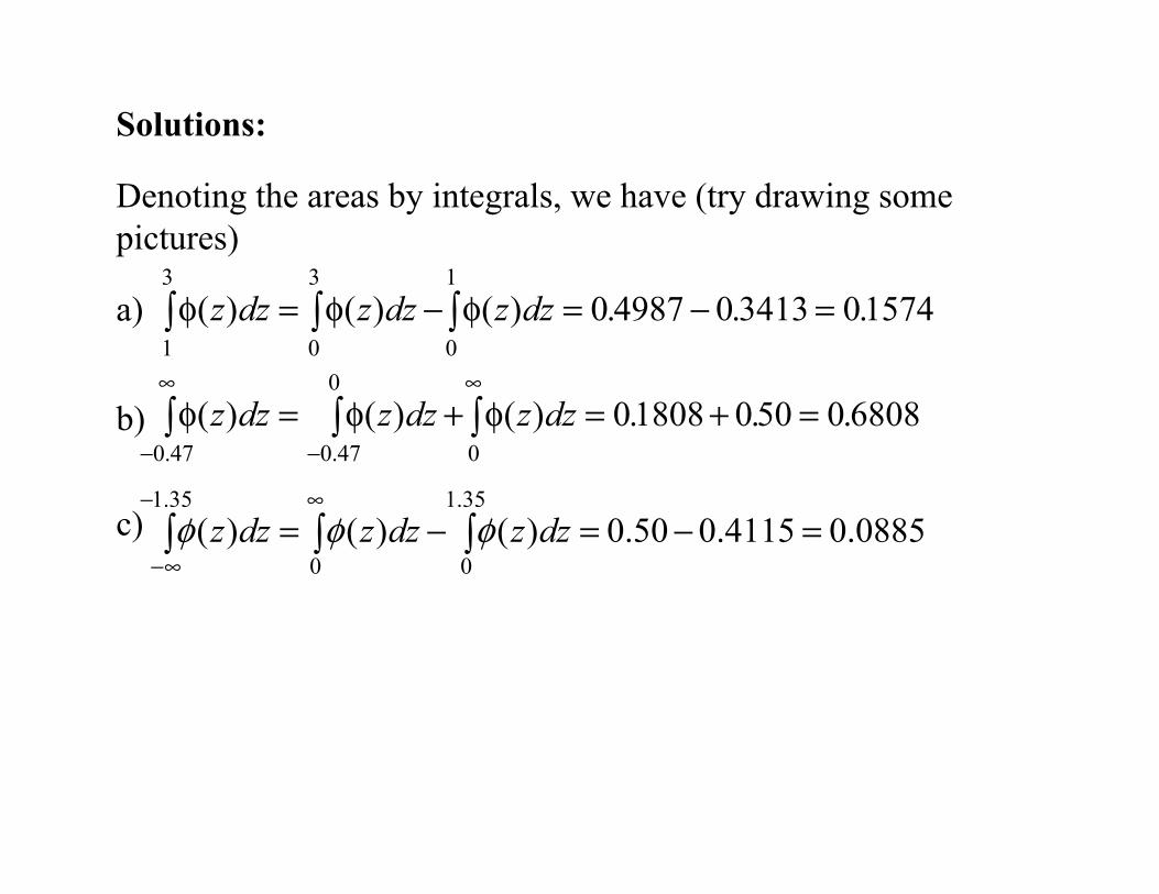
Solutions:

Denoting the areas by integrals, we have (try drawing some pictures)

a)

b)

c)

φ φ φ( ) ( ) ( ) . . .. .

z dz z dz z dz−

∞

−

∞

∫ ∫ ∫= + = + =0 47 0 47

0

001808 0 50 0 6808

0885.04115.050.0)()()(35.1

00

35.1=−=−= ∫∫∫

∞−

∞−dzzdzzdzz φφφ

φ φ φ( ) ( ) ( ) . . .z dz z dz z dz1

3

0

3

0

10 4987 0 3413 01574∫ ∫ ∫= − = − =

Eg: What's the 95th percentile of a standard normal distribution?

Solution: Since we've been given the probability and need to figure out the z-value, we have to use Table IV in reverse. Since the 50th percentile of a standard normal distribution is zero, the 95th percentile is clearly greater than zero.

So we need to find the entry inside of Table IV which is as close as possible to 0.45. In this case, there are two numbers which are equally close to 0.45. They are 0.4495 (z=1.64) and 0.4505 (z=1.65).

So the 95th percentile is 1.645. In other words, there is a 95% probability that a standard normal will be less than 1.645.

Eg: z-scores on an IQ test have a standard normal distribution. If your z-score is 2.7, what is your percentile score?

Solution: To figure out what percentile this score is in, we need to find the probability of getting a lower score, and then multiply by 100.

We have Pr(Z<2.7) = 0.5 + 0.4965 = 0.9965. So the percentile score is 99.65.

Suppose X is normal with mean µ and variance σ2. Any probability involving X can be computed by converting to the z-score, where Z = (X−µ)/σ.

Eg: If the mean IQ score for all test-takers is 100 and the standard deviation is 10, what is the z-score of someone with a raw IQ score of 127?

The z-score defined above measures how many standard deviations X is from its mean.

The z-score is the most appropriate way to express distances from the mean. For example, being 27 points above the mean is fantastic if the standard deviation is 10, but not so great if the standard deviation is 20. (z = 2.7, vs. z = 1.35).

Converting to z-scores

Important Property: If X is normal, then Z = (X−µ)/σ is standard normal, that is, E(Z) = 0, Var(Z) = 1.

Therefore, P(a<X<b) can be computed by finding the probability that a standard normal is between the two corresponding z-scores, (a−µ)/σ and (b−µ)/σ .

Fortunately, we only need one normal table: the one for the standard normal. This makes sense, since all normal distributions have the same shape. Things would be much more complicated if we needed a different table for each value of µ and σ!

•For any normal random variable, we can compute the probability that it will be within 1,2,3 standard deviations of its mean.

This is the same as the probability that the z-score will be within 1,2,3 units from zero. (Why?) Since Z is standard normal, the corresponding probabilities are 0.6826, 0.9544, 0.9974, as computed earlier.

• Thus, the “empirical rule” is exactly correct for any normal random variable.

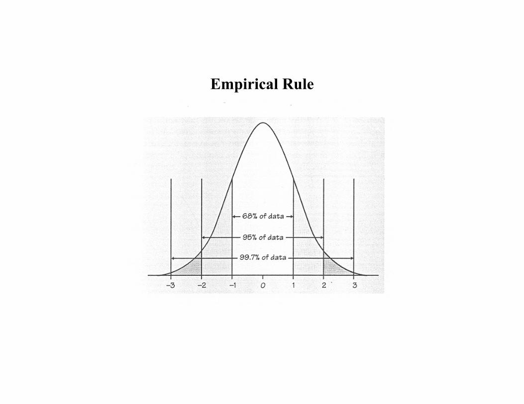
Empirical Rule

Eg 1: Suppose the current price of gold is $370/Ounce. Suppose also that the price 1 month from today has a normal distributionwith mean µ=370 and standard deviation σ=15 (obtained from recent estimates of volatility).

Compute the probability that the price in 1 month will be at or below $350/Ounce.

Eg 2: Scores on the SAT for verbal ability of high school seniors are normally distributed with a mean of 430 and a variance of 10,000.

a) What is the probability that a randomly selected student's score is at most 680?

b) At least 300?c) Between 400 and 540?d) Below what score do 95% of the scores lie?

Eg 3: A company manufactures 1/8” rivets for use in an airplane wing. Due to imperfections in the manufacturing process, the diameters of the rivets are actually normally distributed with mean µ =1/8” and standard deviation σ. In order for the rivets to fit properly into the wing, their diameters must meet the 1/8” target to within a tolerance of ±0.01". To what extent must the company control the variation in the manufacturing process to ensure that at least 95% of all rivets will fit properly?

How can we decide whether a data set came from a normal distribution? First, we can look at the histogram. It should look reasonably symmetric and bell-shaped. If the histogram shows appreciable skewness, then the distribution is not normal. (Normal distributions are symmetric; no skewness).

Unfortunately, the histogram alone is not a sufficient check on normality, since there are many non-normal distributions which are symmetric and bell-shaped.

(An example is the t-distributions).

Checking for Normality in Data

Another useful tool is the boxplot. If the boxplot shows a largenumber of outliers, we might suspect that the distribution is not normal. (Outliers are not always easy to see on a histogram.)If the median is not halfway between the 25th and 75th

percentile, the distribution is skewed. Thus, the boxplot can identify skewness as well as outliers.

Data sets generated by a normal distribution will have almost no outliers. For example, the probability that the absolute value of a standard normal will exceed 4 is just 0.0000633, orapproximately 1 out of 16,000.

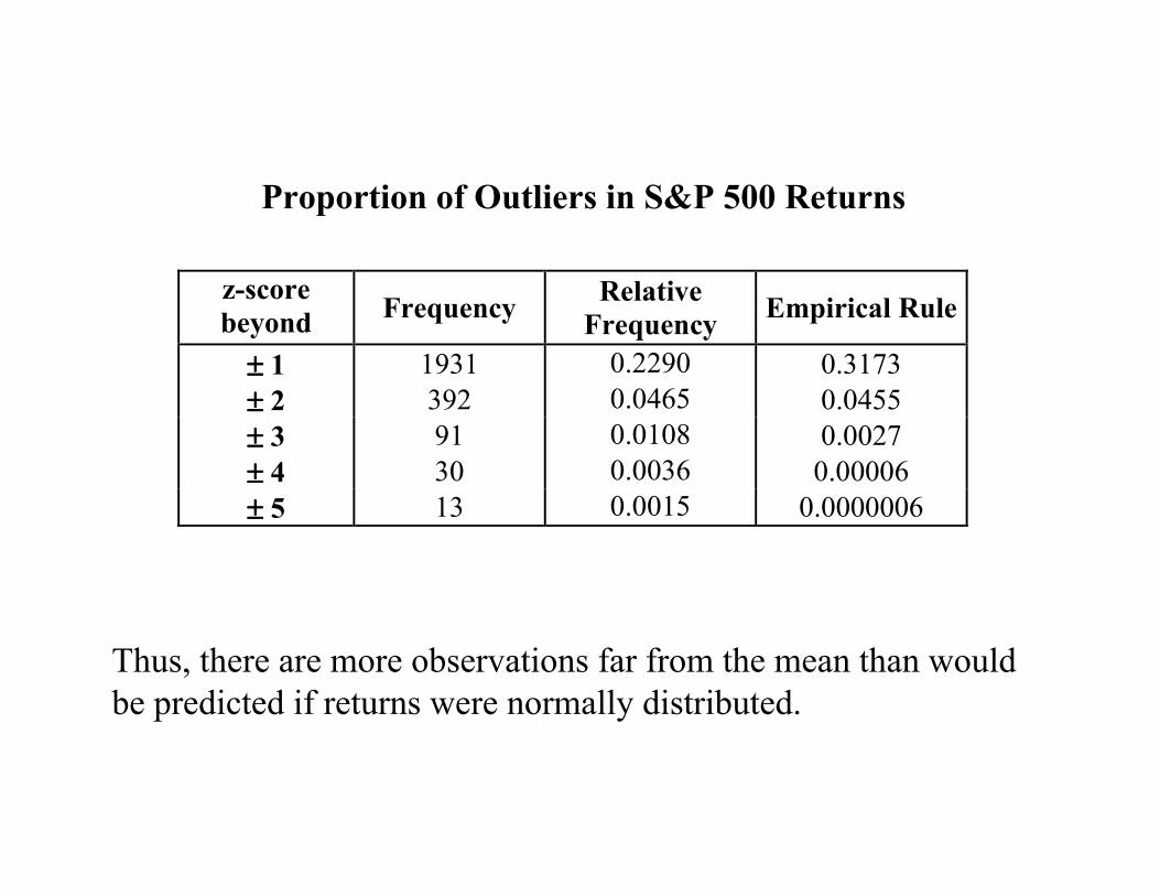
Proportion of Outliers in S&P 500 Returns

Thus, there are more observations far from the mean than would be predicted if returns were normally distributed.

z-scorebeyond Frequency Relative

Frequency Empirical Rule

±±±± 1 1931 0.2290 0.3173±±±± 2 392 0.0465 0.0455±±±± 3 91 0.0108 0.0027±±±± 4 30 0.0036 0.00006±±±± 5 13 0.0015 0.0000006

-0.195-0.170-0.145-0.120-0.095-0.070-0.045-0.0200.0050.0300.0550.080

95% Conf idence Interv al f or Mu

0.0001 0.0002 0.0003 0.0004 0.0005

95% Conf idence Interv al f or Median

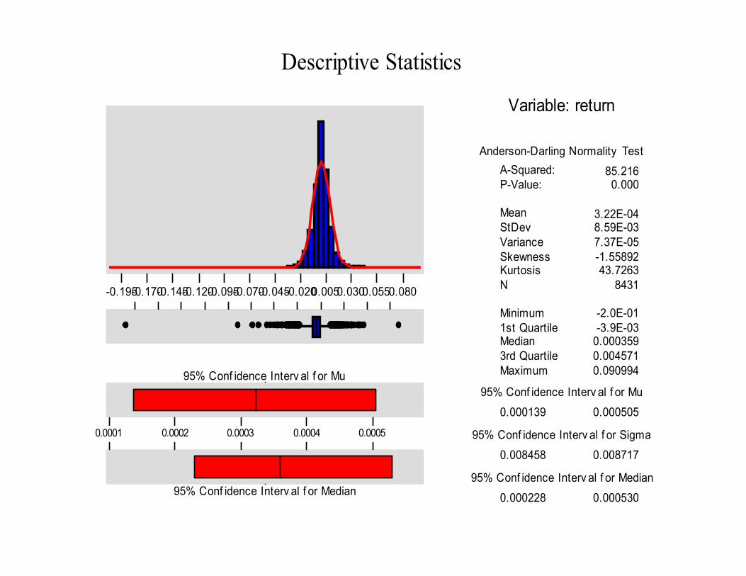
Variable: return

A-Squared:P-Value:

MeanStDevVarianceSkewnessKurtosisN

Minimum1st QuartileMedian3rd QuartileMaximum

0.000139

0.008458

0.000228

85.216 0.000

3.22E-048.59E-037.37E-05-1.5589243.7263

8431

-2.0E-01-3.9E-03

0.0003590.0045710.090994

0.000505

0.008717

0.000530

Anderson-Darling Normality Test

95% Conf idence Interv al f or Mu

95% Conf idence Interv al f or Sigma

95% Conf idence Interv al f or Median

Descriptive Statistics

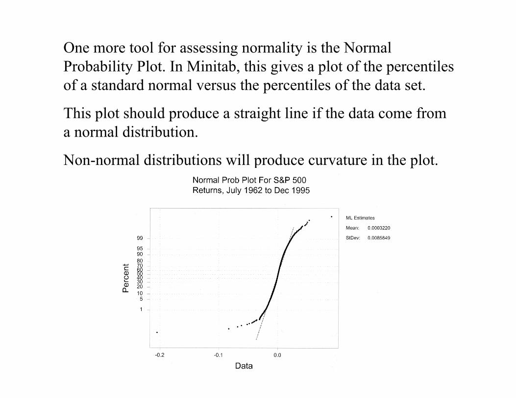
One more tool for assessing normality is the Normal Probability Plot. In Minitab, this gives a plot of the percentiles of a standard normal versus the percentiles of the data set.

This plot should produce a straight line if the data come from a normal distribution.

Non-normal distributions will produce curvature in the plot.

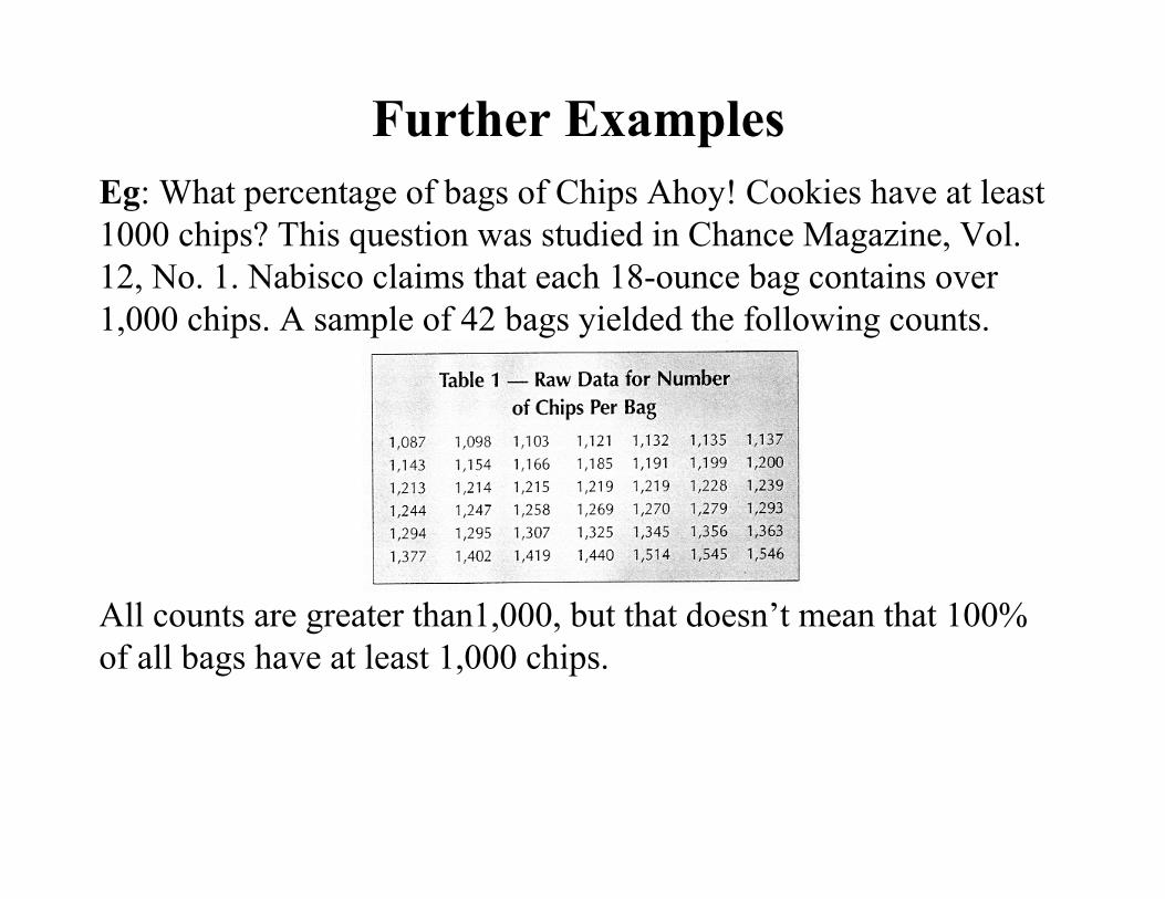
Further ExamplesEg: What percentage of bags of Chips Ahoy! Cookies have at least 1000 chips? This question was studied in Chance Magazine, Vol. 12, No. 1. Nabisco claims that each 18-ounce bag contains over 1,000 chips. A sample of 42 bags yielded the following counts.

All counts are greater than1,000, but that doesn’t mean that 100% of all bags have at least 1,000 chips.

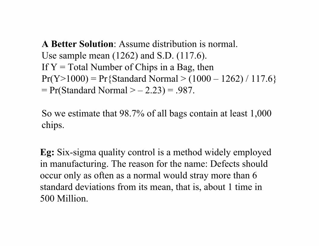
Eg: Six-sigma quality control is a method widely employed in manufacturing. The reason for the name: Defects should occur only as often as a normal would stray more than 6 standard deviations from its mean, that is, about 1 time in 500 Million.

A Better Solution: Assume distribution is normal. Use sample mean (1262) and S.D. (117.6). If Y = Total Number of Chips in a Bag, thenPr(Y>1000) = Pr{Standard Normal > (1000 – 1262) / 117.6} = Pr(Standard Normal > – 2.23) = .987.

So we estimate that 98.7% of all bags contain at least 1,000 chips.

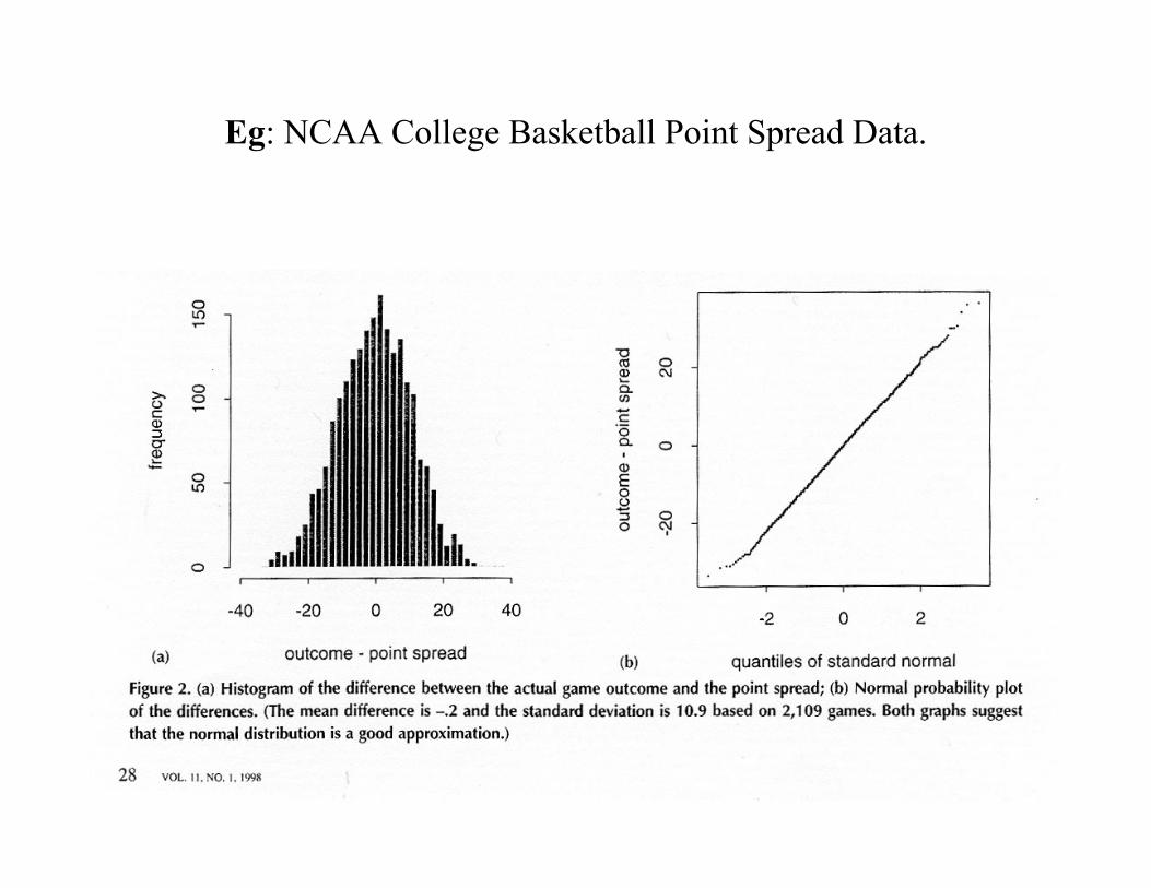
Eg: NCAA College Basketball Point Spread Data.

[Sampling Lab]