16 rounding data + dynamic programming · 16 rounding data + dynamic programming knapsack: given a...
TRANSCRIPT
16 Rounding Data + Dynamic Programming
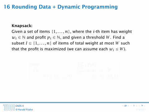
Knapsack:
Given a set of items {1, . . . , n}, where the i-th item has weight
wi ∈ N and profit pi ∈ N, and given a threshold W . Find a
subset I ⊆ {1, . . . , n} of items of total weight at most W such
that the profit is maximized (we can assume each wi ≤ W ).
max∑ni=1 pixi
s.t.∑ni=1wixi ≤ W
∀i ∈ {1, . . . , n} xi ∈ {0,1}
EADS II
© Harald Räcke 319/521

16 Rounding Data + Dynamic Programming
Knapsack:
Given a set of items {1, . . . , n}, where the i-th item has weight
wi ∈ N and profit pi ∈ N, and given a threshold W . Find a
subset I ⊆ {1, . . . , n} of items of total weight at most W such
that the profit is maximized (we can assume each wi ≤ W ).
max∑ni=1 pixi
s.t.∑ni=1wixi ≤ W
∀i ∈ {1, . . . , n} xi ∈ {0,1}
EADS II 16.1 Knapsack
© Harald Räcke 319/521
16 Rounding Data + Dynamic Programming
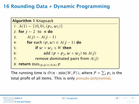
Algorithm 1 Knapsack
1: A(1)← [(0,0), (p1,w1)]2: for j ← 2 to n do
3: A(j)← A(j − 1)4: for each (p,w) ∈ A(j − 1) do
5: if w +wj ≤ W then
6: add (p + pj ,w +wj) to A(j)7: remove dominated pairs from A(j)8: return max(p,w)∈A(n) p
The running time is O(n ·min{W,P}), where P =∑i pi is the
total profit of all items. This is only pseudo-polynomial.
EADS II 16.1 Knapsack
© Harald Räcke 320/521
16 Rounding Data + Dynamic Programming
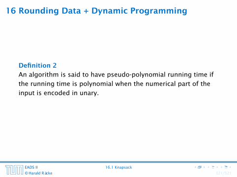
Definition 2
An algorithm is said to have pseudo-polynomial running time if
the running time is polynomial when the numerical part of the
input is encoded in unary.
EADS II 16.1 Knapsack
© Harald Räcke 321/521

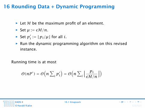
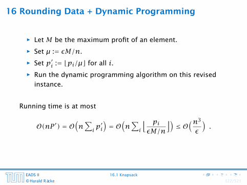
16 Rounding Data + Dynamic Programming
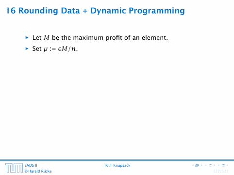
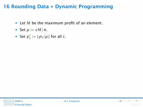
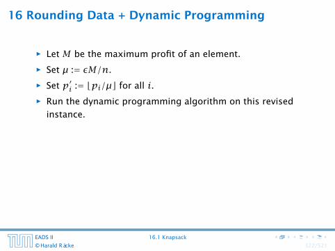
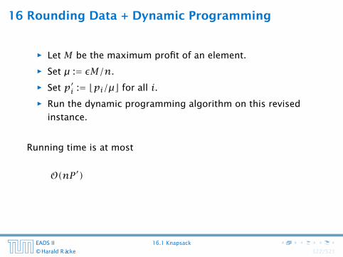
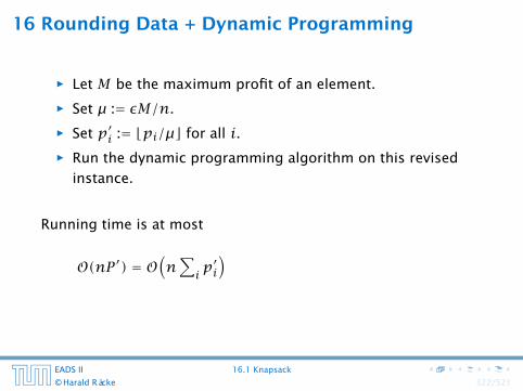
ñ Let M be the maximum profit of an element.
ñ Set µ := εM/n.
ñ Set p′i := bpi/µc for all i.ñ Run the dynamic programming algorithm on this revised
instance.
Running time is at most
O(nP ′) = O(n∑i p′i
)= O
(n∑i
⌊ piεM/n
⌋)≤ O
(n3
ε
).
EADS II 16.1 Knapsack
© Harald Räcke 322/521
16 Rounding Data + Dynamic Programming
ñ Let M be the maximum profit of an element.
ñ Set µ := εM/n.
ñ Set p′i := bpi/µc for all i.
ñ Run the dynamic programming algorithm on this revised
instance.
Running time is at most
O(nP ′) = O(n∑i p′i
)= O
(n∑i
⌊ piεM/n
⌋)≤ O
(n3
ε
).
EADS II 16.1 Knapsack
© Harald Räcke 322/521
16 Rounding Data + Dynamic Programming
ñ Let M be the maximum profit of an element.
ñ Set µ := εM/n.
ñ Set p′i := bpi/µc for all i.ñ Run the dynamic programming algorithm on this revised
instance.
Running time is at most
O(nP ′) = O(n∑i p′i
)= O
(n∑i
⌊ piεM/n
⌋)≤ O
(n3
ε
).
EADS II 16.1 Knapsack
© Harald Räcke 322/521
16 Rounding Data + Dynamic Programming
ñ Let M be the maximum profit of an element.
ñ Set µ := εM/n.
ñ Set p′i := bpi/µc for all i.ñ Run the dynamic programming algorithm on this revised
instance.
Running time is at most
O(nP ′)
= O(n∑i p′i
)= O
(n∑i
⌊ piεM/n
⌋)≤ O
(n3
ε
).
EADS II 16.1 Knapsack
© Harald Räcke 322/521
16 Rounding Data + Dynamic Programming
ñ Let M be the maximum profit of an element.
ñ Set µ := εM/n.
ñ Set p′i := bpi/µc for all i.ñ Run the dynamic programming algorithm on this revised
instance.
Running time is at most
O(nP ′) = O(n∑i p′i
)
= O(n∑i
⌊ piεM/n
⌋)≤ O
(n3
ε
).
EADS II 16.1 Knapsack
© Harald Räcke 322/521
16 Rounding Data + Dynamic Programming
ñ Let M be the maximum profit of an element.
ñ Set µ := εM/n.
ñ Set p′i := bpi/µc for all i.ñ Run the dynamic programming algorithm on this revised
instance.
Running time is at most
O(nP ′) = O(n∑i p′i
)= O
(n∑i
⌊ piεM/n
⌋)
≤ O(n3
ε
).
EADS II 16.1 Knapsack
© Harald Räcke 322/521
16 Rounding Data + Dynamic Programming
ñ Let M be the maximum profit of an element.
ñ Set µ := εM/n.
ñ Set p′i := bpi/µc for all i.ñ Run the dynamic programming algorithm on this revised
instance.
Running time is at most
O(nP ′) = O(n∑i p′i
)= O
(n∑i
⌊ piεM/n
⌋)≤ O
(n3
ε
).
EADS II 16.1 Knapsack
© Harald Räcke 322/521
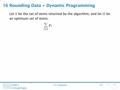
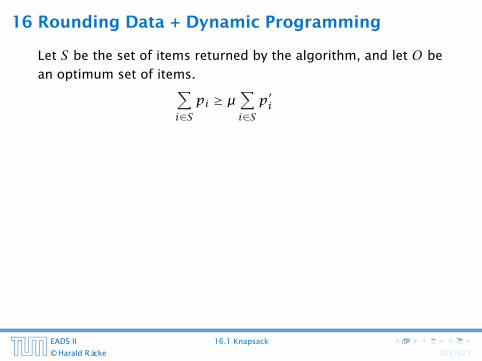
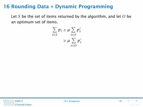
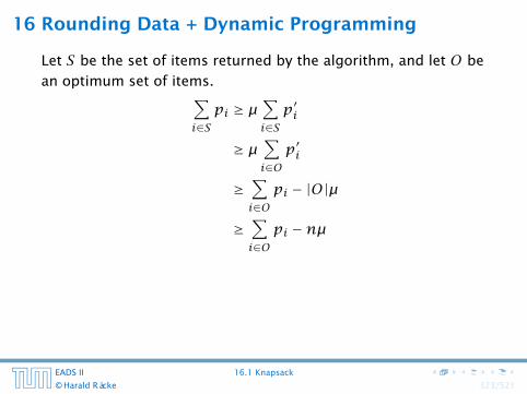
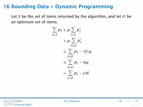
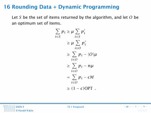
16 Rounding Data + Dynamic Programming
Let S be the set of items returned by the algorithm, and let O be
an optimum set of items.∑i∈Spi
≥ µ∑i∈Sp′i
≥ µ∑i∈Op′i
≥∑i∈Opi − |O|µ
≥∑i∈Opi −nµ
=∑i∈Opi − εM
≥ (1− ε)OPT .
EADS II 16.1 Knapsack
© Harald Räcke 323/521
16 Rounding Data + Dynamic Programming
Let S be the set of items returned by the algorithm, and let O be
an optimum set of items.∑i∈Spi ≥ µ
∑i∈Sp′i
≥ µ∑i∈Op′i
≥∑i∈Opi − |O|µ
≥∑i∈Opi −nµ
=∑i∈Opi − εM
≥ (1− ε)OPT .
EADS II 16.1 Knapsack
© Harald Räcke 323/521
16 Rounding Data + Dynamic Programming
Let S be the set of items returned by the algorithm, and let O be
an optimum set of items.∑i∈Spi ≥ µ
∑i∈Sp′i
≥ µ∑i∈Op′i
≥∑i∈Opi − |O|µ
≥∑i∈Opi −nµ
=∑i∈Opi − εM
≥ (1− ε)OPT .
EADS II 16.1 Knapsack
© Harald Räcke 323/521

16 Rounding Data + Dynamic Programming
Let S be the set of items returned by the algorithm, and let O be
an optimum set of items.∑i∈Spi ≥ µ
∑i∈Sp′i
≥ µ∑i∈Op′i
≥∑i∈Opi − |O|µ
≥∑i∈Opi −nµ
=∑i∈Opi − εM
≥ (1− ε)OPT .
EADS II 16.1 Knapsack
© Harald Räcke 323/521
16 Rounding Data + Dynamic Programming
Let S be the set of items returned by the algorithm, and let O be
an optimum set of items.∑i∈Spi ≥ µ
∑i∈Sp′i
≥ µ∑i∈Op′i
≥∑i∈Opi − |O|µ
≥∑i∈Opi −nµ
=∑i∈Opi − εM
≥ (1− ε)OPT .
EADS II 16.1 Knapsack
© Harald Räcke 323/521
16 Rounding Data + Dynamic Programming
Let S be the set of items returned by the algorithm, and let O be
an optimum set of items.∑i∈Spi ≥ µ
∑i∈Sp′i
≥ µ∑i∈Op′i
≥∑i∈Opi − |O|µ
≥∑i∈Opi −nµ
=∑i∈Opi − εM
≥ (1− ε)OPT .
EADS II 16.1 Knapsack
© Harald Räcke 323/521
16 Rounding Data + Dynamic Programming
Let S be the set of items returned by the algorithm, and let O be
an optimum set of items.∑i∈Spi ≥ µ
∑i∈Sp′i
≥ µ∑i∈Op′i
≥∑i∈Opi − |O|µ
≥∑i∈Opi −nµ
=∑i∈Opi − εM
≥ (1− ε)OPT .
EADS II 16.1 Knapsack
© Harald Räcke 323/521
Scheduling Revisited
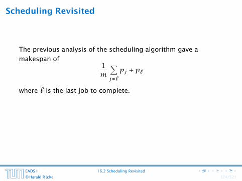
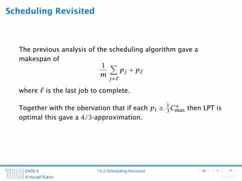
The previous analysis of the scheduling algorithm gave a
makespan of1m
∑j≠`
pj + p`
where ` is the last job to complete.
Together with the obervation that if each pi ≥ 13C∗max then LPT is
optimal this gave a 4/3-approximation.
EADS II 16.2 Scheduling Revisited
© Harald Räcke 324/521
Scheduling Revisited
The previous analysis of the scheduling algorithm gave a
makespan of1m
∑j≠`
pj + p`
where ` is the last job to complete.
Together with the obervation that if each pi ≥ 13C∗max then LPT is
optimal this gave a 4/3-approximation.
EADS II 16.2 Scheduling Revisited
© Harald Räcke 324/521
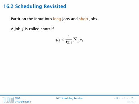
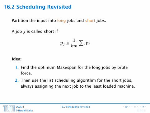
16.2 Scheduling Revisited
Partition the input into long jobs and short jobs.
A job j is called short if
pj ≤1km
∑i pi
Idea:
1. Find the optimum Makespan for the long jobs by brute
force.
2. Then use the list scheduling algorithm for the short jobs,
always assigning the next job to the least loaded machine.
EADS II 16.2 Scheduling Revisited
© Harald Räcke 325/521

We still have the inequality
1m
∑j≠`
pj + p`
where ` is the last job (this only requires that all machines are
busy before time S`).
If ` is a long job, then the schedule must be optimal, as it
consists of an optimal schedule of long jobs plus a schedule for
short jobs.
If ` is a short job its length is at most
p` ≤∑j pj/(mk)
which is at most C∗max/k.
EADS II 16.2 Scheduling Revisited
© Harald Räcke 326/521
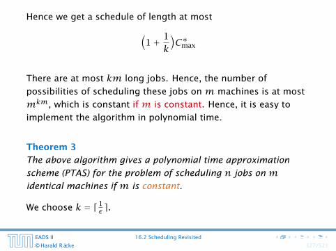
Hence we get a schedule of length at most(1+ 1
k
)C∗max
There are at most km long jobs. Hence, the number of
possibilities of scheduling these jobs on m machines is at most
mkm, which is constant if m is constant. Hence, it is easy to
implement the algorithm in polynomial time.
Theorem 3
The above algorithm gives a polynomial time approximation
scheme (PTAS) for the problem of scheduling n jobs on midentical machines if m is constant.
We choose k = d1ε e.
EADS II 16.2 Scheduling Revisited
© Harald Räcke 327/521
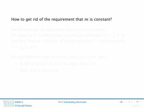
How to get rid of the requirement that m is constant?
We first design an algorithm that works as follows:
On input of T it either finds a schedule of length (1+ 1k)T or
certifies that no schedule of length at most T exists (assume
T ≥ 1m∑j pj).
We partition the jobs into long jobs and short jobs:
ñ A job is long if its size is larger than T/k.
ñ Otw. it is a short job.
EADS II 16.2 Scheduling Revisited
© Harald Räcke 328/521

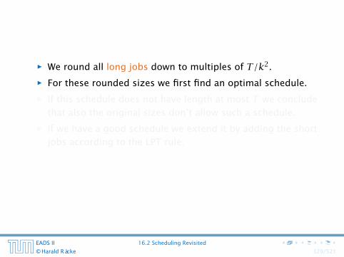
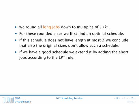
ñ We round all long jobs down to multiples of T/k2.
ñ For these rounded sizes we first find an optimal schedule.
ñ If this schedule does not have length at most T we conclude
that also the original sizes don’t allow such a schedule.
ñ If we have a good schedule we extend it by adding the short
jobs according to the LPT rule.
EADS II 16.2 Scheduling Revisited
© Harald Räcke 329/521
After the first phase the rounded sizes of the long jobs assigned
to a machine add up to at most T .
There can be at most k (long) jobs assigned to a machine as otw.
their rounded sizes would add up to more than T (note that the
rounded size of a long job is at least T/k).
Since, jobs had been rounded to multiples of T/k2 going from
rounded sizes to original sizes gives that the Makespan is at
most (1+ 1
k
)T .
EADS II 16.2 Scheduling Revisited
© Harald Räcke 330/521

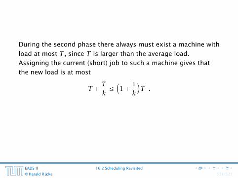
During the second phase there always must exist a machine with
load at most T , since T is larger than the average load.
Assigning the current (short) job to such a machine gives that
the new load is at most
T + Tk≤(1+ 1
k
)T .
EADS II 16.2 Scheduling Revisited
© Harald Räcke 331/521
During the second phase there always must exist a machine with
load at most T , since T is larger than the average load.
Assigning the current (short) job to such a machine gives that
the new load is at most
T + Tk≤(1+ 1
k
)T .
EADS II 16.2 Scheduling Revisited
© Harald Räcke 331/521
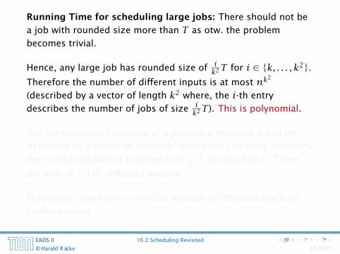
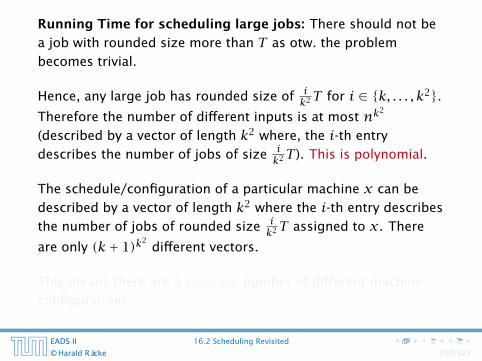
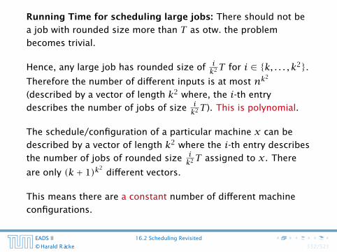
Running Time for scheduling large jobs: There should not be
a job with rounded size more than T as otw. the problem
becomes trivial.
Hence, any large job has rounded size of ik2T for i ∈ {k, . . . , k2}.
Therefore the number of different inputs is at most nk2
(described by a vector of length k2 where, the i-th entry
describes the number of jobs of size ik2T ). This is polynomial.
The schedule/configuration of a particular machine x can be
described by a vector of length k2 where the i-th entry describes
the number of jobs of rounded size ik2T assigned to x. There
are only (k+ 1)k2different vectors.
This means there are a constant number of different machine
configurations.
EADS II 16.2 Scheduling Revisited
© Harald Räcke 332/521
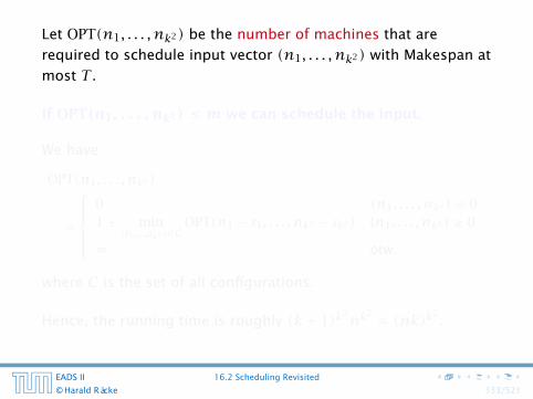
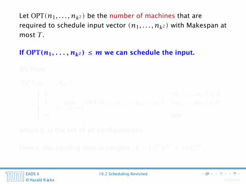
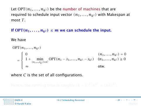
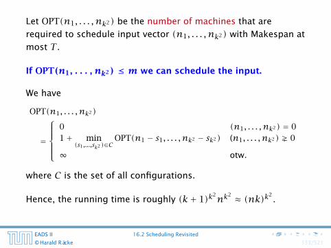
Let OPT(n1, . . . , nk2) be the number of machines that are
required to schedule input vector (n1, . . . , nk2) with Makespan at
most T .
If OPT(n1, . . . , nk2) ≤ m we can schedule the input.
We have
OPT(n1, . . . , nk2)
=
0 (n1, . . . , nk2) = 01+ min
(s1,...,sk2 )∈COPT(n1 − s1, . . . , nk2 − sk2) (n1, . . . , nk2) Û 0
∞ otw.
where C is the set of all configurations.
Hence, the running time is roughly (k+ 1)k2nk2 ≈ (nk)k2.
EADS II 16.2 Scheduling Revisited
© Harald Räcke 333/521
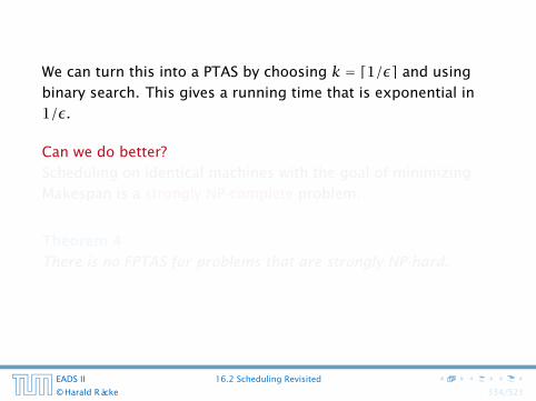
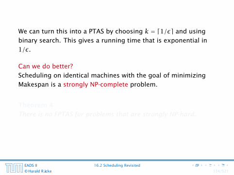
We can turn this into a PTAS by choosing k = d1/εe and using
binary search. This gives a running time that is exponential in
1/ε.
Can we do better?
Scheduling on identical machines with the goal of minimizing
Makespan is a strongly NP-complete problem.
Theorem 4
There is no FPTAS for problems that are strongly NP-hard.
EADS II 16.2 Scheduling Revisited
© Harald Räcke 334/521
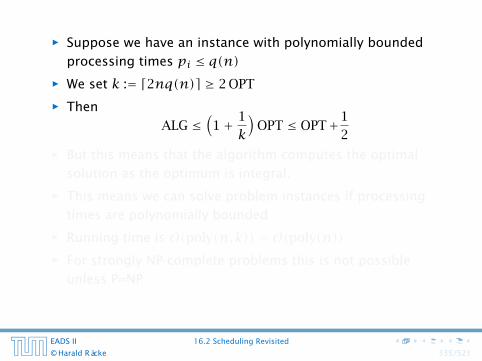
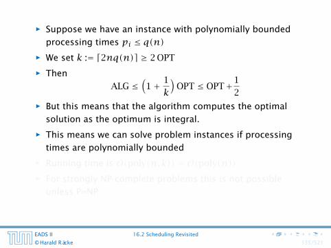
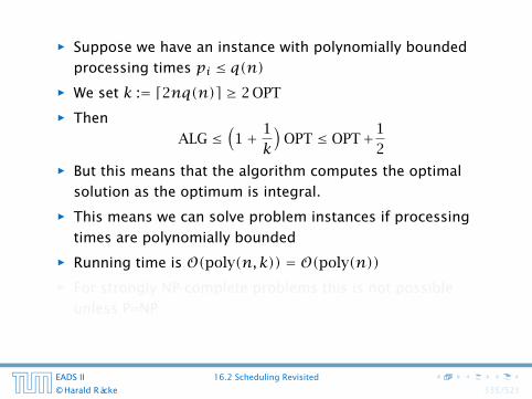
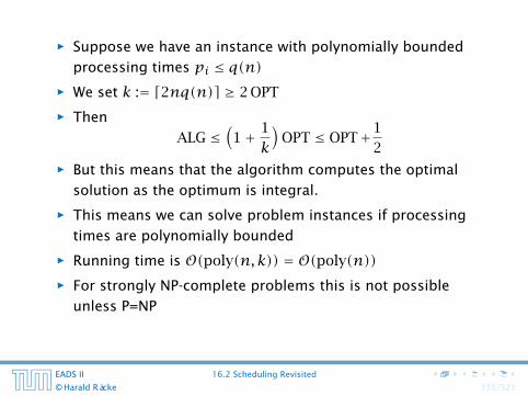
ñ Suppose we have an instance with polynomially bounded
processing times pi ≤ q(n)ñ We set k := d2nq(n)e ≥ 2 OPT
ñ Then
ALG ≤(1+ 1
k
)OPT ≤ OPT+1
2ñ But this means that the algorithm computes the optimal
solution as the optimum is integral.
ñ This means we can solve problem instances if processing
times are polynomially bounded
ñ Running time is O(poly(n, k)) = O(poly(n))ñ For strongly NP-complete problems this is not possible
unless P=NP
EADS II 16.2 Scheduling Revisited
© Harald Räcke 335/521
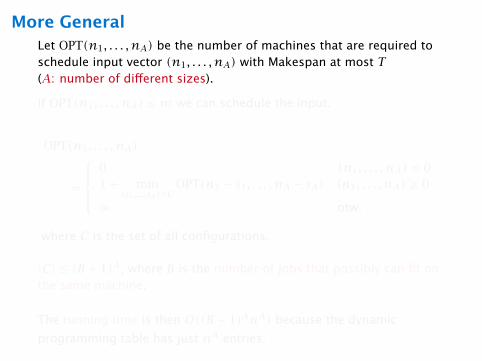
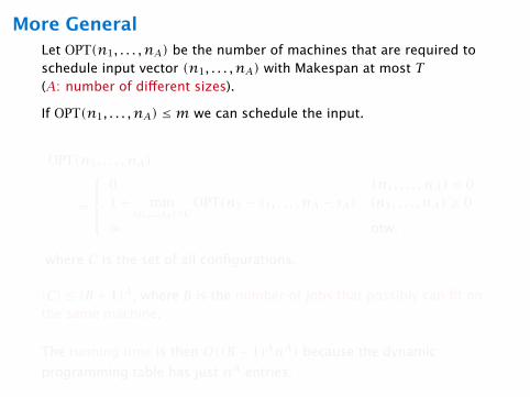
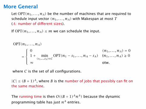
More GeneralLet OPT(n1, . . . , nA) be the number of machines that are required toschedule input vector (n1, . . . , nA) with Makespan at most T(A: number of different sizes).
If OPT(n1, . . . , nA) ≤m we can schedule the input.
OPT(n1, . . . , nA)
=
0 (n1, . . . , nA) = 01+ min
(s1,...,sA)∈COPT(n1 − s1, . . . , nA − sA) (n1, . . . , nA) Û 0
∞ otw.
where C is the set of all configurations.
|C| ≤ (B + 1)A, where B is the number of jobs that possibly can fit onthe same machine.
The running time is then O((B + 1)AnA) because the dynamic
programming table has just nA entries.
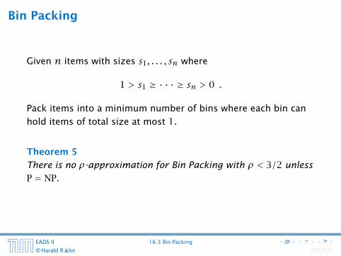
Bin Packing
Given n items with sizes s1, . . . , sn where
1 > s1 ≥ · · · ≥ sn > 0 .
Pack items into a minimum number of bins where each bin can
hold items of total size at most 1.
Theorem 5
There is no ρ-approximation for Bin Packing with ρ < 3/2 unless
P = NP.
EADS II 16.3 Bin Packing
© Harald Räcke 337/521
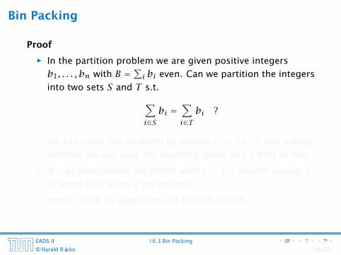
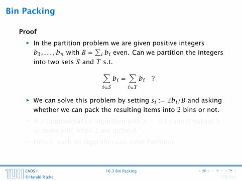
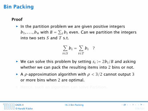
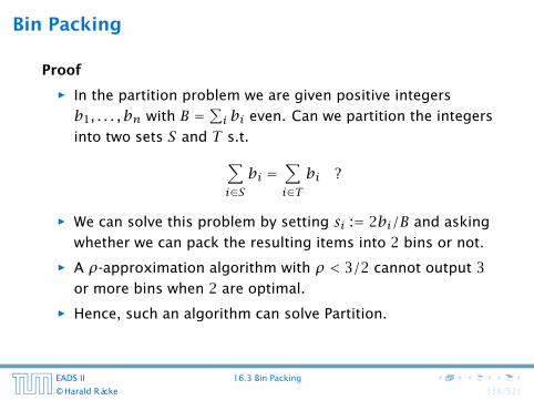
Bin Packing
Proof
ñ In the partition problem we are given positive integers
b1, . . . , bn with B =∑i bi even. Can we partition the integers
into two sets S and T s.t.∑i∈Sbi =
∑i∈Tbi ?
ñ We can solve this problem by setting si := 2bi/B and asking
whether we can pack the resulting items into 2 bins or not.
ñ A ρ-approximation algorithm with ρ < 3/2 cannot output 3
or more bins when 2 are optimal.
ñ Hence, such an algorithm can solve Partition.
EADS II 16.3 Bin Packing
© Harald Räcke 338/521
Bin Packing
Definition 6
An asymptotic polynomial-time approximation scheme (APTAS)
is a family of algorithms {Aε} along with a constant c such that
Aε returns a solution of value at most (1+ ε)OPT+ c for
minimization problems.
ñ Note that for Set Cover or for Knapsack it makes no sense
to differentiate between the notion of a PTAS or an APTAS
because of scaling.
ñ However, we will develop an APTAS for Bin Packing.
EADS II 16.3 Bin Packing
© Harald Räcke 339/521
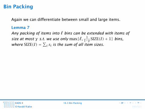
Bin Packing
Again we can differentiate between small and large items.
Lemma 7
Any packing of items into ` bins can be extended with items of
size at most γ s.t. we use only max{`, 11−γ SIZE(I)+ 1} bins,
where SIZE(I) =∑i si is the sum of all item sizes.
ñ If after Greedy we use more than ` bins, all bins (apart from
the last) must be full to at least 1− γ.
ñ Hence, r(1− γ) ≤ SIZE(I) where r is the number of
nearly-full bins.
ñ This gives the lemma.
EADS II 16.3 Bin Packing
© Harald Räcke 340/521
Choose γ = ε/2. Then we either use ` bins or at most
11− ε/2 ·OPT+ 1 ≤ (1+ ε) ·OPT+ 1
bins.
It remains to find an algorithm for the large items.
EADS II 16.3 Bin Packing
© Harald Räcke 341/521
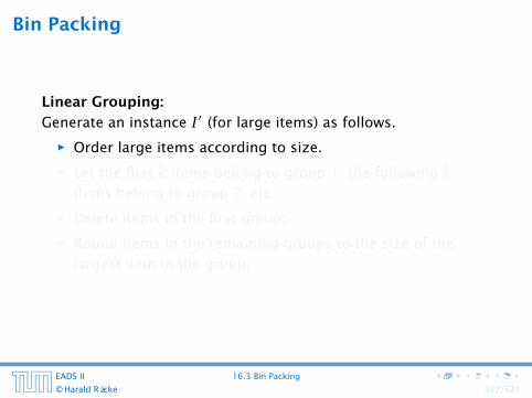
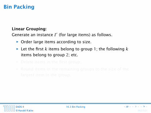
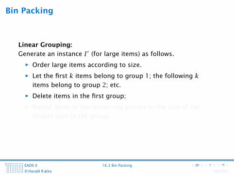
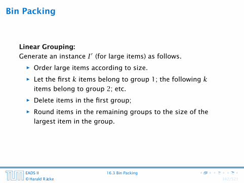
Bin Packing
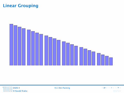
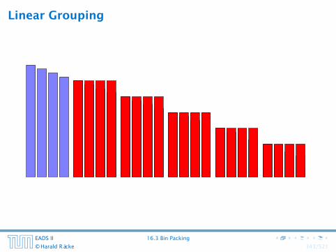
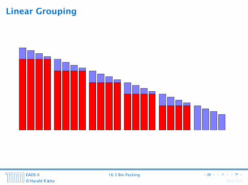
Linear Grouping:
Generate an instance I′ (for large items) as follows.
ñ Order large items according to size.
ñ Let the first k items belong to group 1; the following kitems belong to group 2; etc.
ñ Delete items in the first group;
ñ Round items in the remaining groups to the size of the
largest item in the group.
EADS II 16.3 Bin Packing
© Harald Räcke 342/521
Bin Packing
Linear Grouping:
Generate an instance I′ (for large items) as follows.
ñ Order large items according to size.
ñ Let the first k items belong to group 1; the following kitems belong to group 2; etc.
ñ Delete items in the first group;
ñ Round items in the remaining groups to the size of the
largest item in the group.
EADS II 16.3 Bin Packing
© Harald Räcke 342/521
Linear Grouping
EADS II 16.3 Bin Packing
© Harald Räcke 343/521
Linear Grouping
EADS II 16.3 Bin Packing
© Harald Räcke 343/521

Linear Grouping
EADS II 16.3 Bin Packing
© Harald Räcke 343/521
Linear Grouping
EADS II 16.3 Bin Packing
© Harald Räcke 343/521
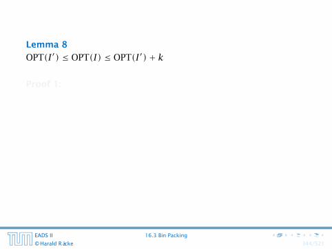
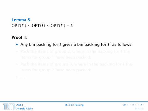
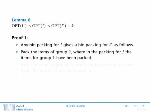
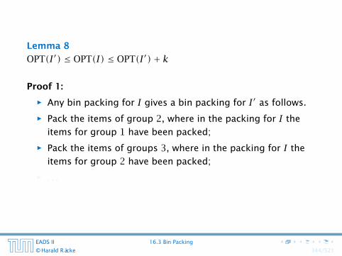
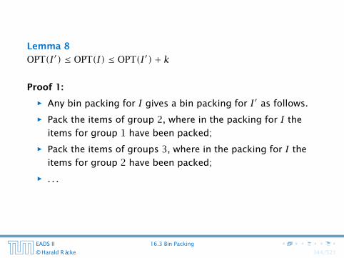
Lemma 8
OPT(I′) ≤ OPT(I) ≤ OPT(I′)+ k
Proof 1:
ñ Any bin packing for I gives a bin packing for I′ as follows.
ñ Pack the items of group 2, where in the packing for I the
items for group 1 have been packed;
ñ Pack the items of groups 3, where in the packing for I the
items for group 2 have been packed;
ñ . . .
EADS II 16.3 Bin Packing
© Harald Räcke 344/521
Lemma 9
OPT(I′) ≤ OPT(I) ≤ OPT(I′)+ k
Proof 2:
ñ Any bin packing for I′ gives a bin packing for I as follows.
ñ Pack the items of group 1 into k new bins;
ñ Pack the items of groups 2, where in the packing for I′ the
items for group 2 have been packed;
ñ . . .
EADS II 16.3 Bin Packing
© Harald Räcke 345/521
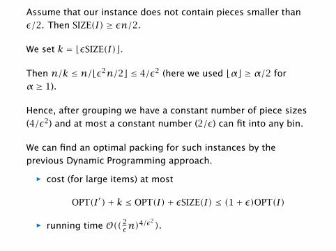
Assume that our instance does not contain pieces smaller than
ε/2. Then SIZE(I) ≥ εn/2.
We set k = bεSIZE(I)c.
Then n/k ≤ n/bε2n/2c ≤ 4/ε2 (here we used bαc ≥ α/2 for
α ≥ 1).
Hence, after grouping we have a constant number of piece sizes
(4/ε2) and at most a constant number (2/ε) can fit into any bin.
We can find an optimal packing for such instances by the
previous Dynamic Programming approach.
ñ cost (for large items) at most
OPT(I′)+ k ≤ OPT(I)+ εSIZE(I) ≤ (1+ ε)OPT(I)
ñ running time O((2εn)
4/ε2).
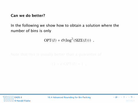
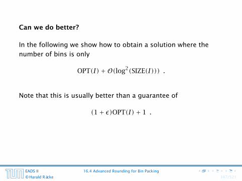
Can we do better?
In the following we show how to obtain a solution where the
number of bins is only
OPT(I)+O(log2(SIZE(I))) .
Note that this is usually better than a guarantee of
(1+ ε)OPT(I)+ 1 .
EADS II 16.4 Advanced Rounding for Bin Packing
© Harald Räcke 347/521
Can we do better?
In the following we show how to obtain a solution where the
number of bins is only
OPT(I)+O(log2(SIZE(I))) .
Note that this is usually better than a guarantee of
(1+ ε)OPT(I)+ 1 .
EADS II 16.4 Advanced Rounding for Bin Packing
© Harald Räcke 347/521
Can we do better?
In the following we show how to obtain a solution where the
number of bins is only
OPT(I)+O(log2(SIZE(I))) .
Note that this is usually better than a guarantee of
(1+ ε)OPT(I)+ 1 .
EADS II 16.4 Advanced Rounding for Bin Packing
© Harald Räcke 347/521
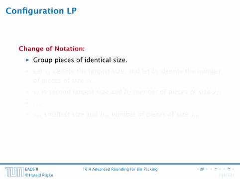
Configuration LP
Change of Notation:
ñ Group pieces of identical size.
ñ Let s1 denote the largest size, and let b1 denote the number
of pieces of size s1.
ñ s2 is second largest size and b2 number of pieces of size s2;
ñ . . .ñ sm smallest size and bm number of pieces of size sm.
EADS II 16.4 Advanced Rounding for Bin Packing
© Harald Räcke 348/521

Configuration LP
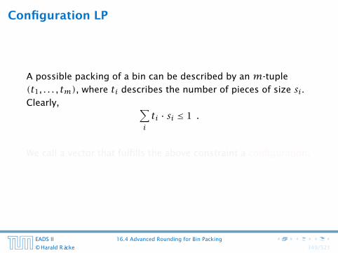
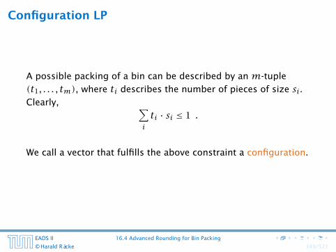
A possible packing of a bin can be described by an m-tuple
(t1, . . . , tm), where ti describes the number of pieces of size si.Clearly, ∑
iti · si ≤ 1 .
We call a vector that fulfills the above constraint a configuration.
EADS II 16.4 Advanced Rounding for Bin Packing
© Harald Räcke 349/521
Configuration LP
A possible packing of a bin can be described by an m-tuple
(t1, . . . , tm), where ti describes the number of pieces of size si.Clearly, ∑
iti · si ≤ 1 .
We call a vector that fulfills the above constraint a configuration.
EADS II 16.4 Advanced Rounding for Bin Packing
© Harald Räcke 349/521

Configuration LP
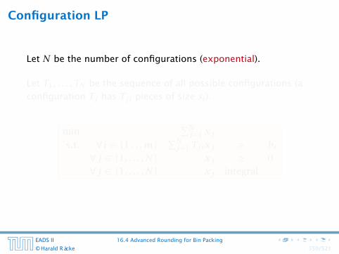
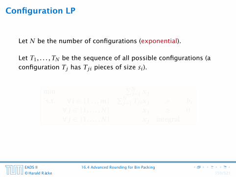
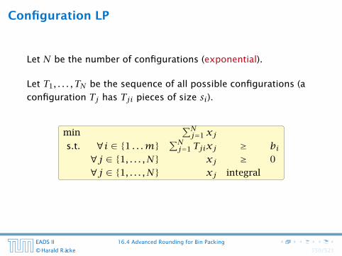
Let N be the number of configurations (exponential).
Let T1, . . . , TN be the sequence of all possible configurations (a
configuration Tj has Tji pieces of size si).
min∑Nj=1 xj
s.t. ∀i ∈ {1 . . .m}∑Nj=1 Tjixj ≥ bi
∀j ∈ {1, . . . ,N} xj ≥ 0
∀j ∈ {1, . . . ,N} xj integral
EADS II 16.4 Advanced Rounding for Bin Packing
© Harald Räcke 350/521
Configuration LP
Let N be the number of configurations (exponential).
Let T1, . . . , TN be the sequence of all possible configurations (a
configuration Tj has Tji pieces of size si).
min∑Nj=1 xj
s.t. ∀i ∈ {1 . . .m}∑Nj=1 Tjixj ≥ bi
∀j ∈ {1, . . . ,N} xj ≥ 0
∀j ∈ {1, . . . ,N} xj integral
EADS II 16.4 Advanced Rounding for Bin Packing
© Harald Räcke 350/521

How to solve this LP?
later...
EADS II 16.4 Advanced Rounding for Bin Packing
© Harald Räcke 351/521
We can assume that each item has size at least 1/SIZE(I).
EADS II 16.4 Advanced Rounding for Bin Packing
© Harald Räcke 352/521
Harmonic Grouping
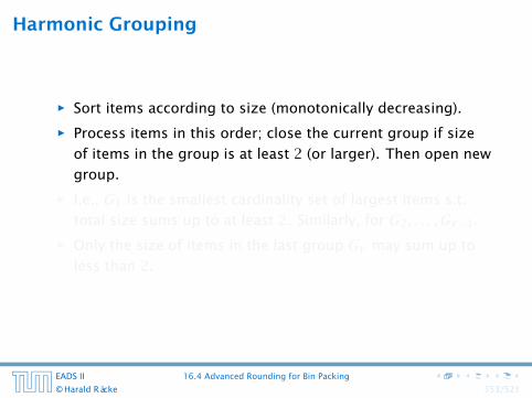
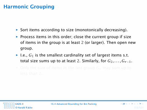
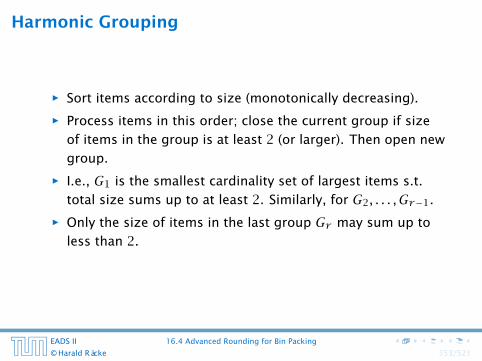
ñ Sort items according to size (monotonically decreasing).
ñ Process items in this order; close the current group if size
of items in the group is at least 2 (or larger). Then open new
group.
ñ I.e., G1 is the smallest cardinality set of largest items s.t.
total size sums up to at least 2. Similarly, for G2, . . . , Gr−1.
ñ Only the size of items in the last group Gr may sum up to
less than 2.
EADS II 16.4 Advanced Rounding for Bin Packing
© Harald Räcke 353/521
Harmonic Grouping
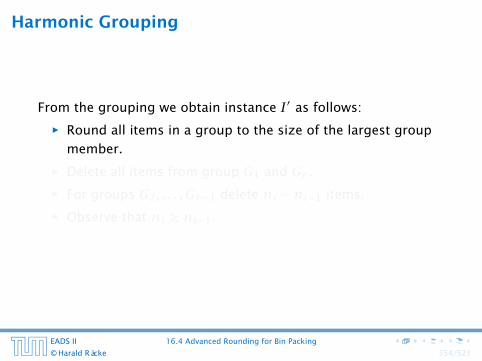
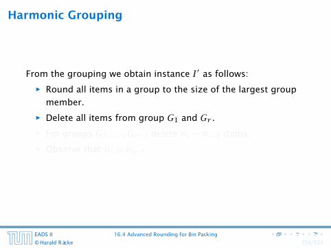
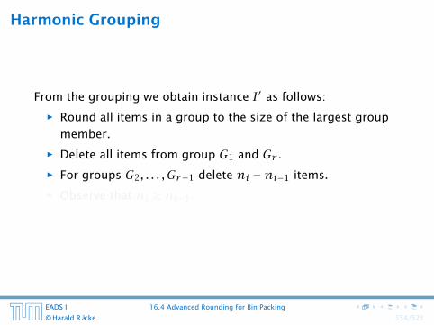
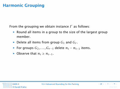
From the grouping we obtain instance I′ as follows:
ñ Round all items in a group to the size of the largest group
member.
ñ Delete all items from group G1 and Gr .ñ For groups G2, . . . , Gr−1 delete ni −ni−1 items.
ñ Observe that ni ≥ ni−1.
EADS II 16.4 Advanced Rounding for Bin Packing
© Harald Räcke 354/521
Harmonic Grouping
From the grouping we obtain instance I′ as follows:
ñ Round all items in a group to the size of the largest group
member.
ñ Delete all items from group G1 and Gr .ñ For groups G2, . . . , Gr−1 delete ni −ni−1 items.
ñ Observe that ni ≥ ni−1.
EADS II 16.4 Advanced Rounding for Bin Packing
© Harald Räcke 354/521
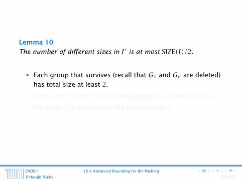
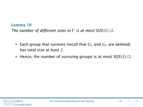
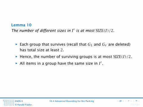
Lemma 10
The number of different sizes in I′ is at most SIZE(I)/2.
ñ Each group that survives (recall that G1 and Gr are deleted)
has total size at least 2.
ñ Hence, the number of surviving groups is at most SIZE(I)/2.
ñ All items in a group have the same size in I′.
EADS II 16.4 Advanced Rounding for Bin Packing
© Harald Räcke 355/521
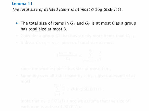
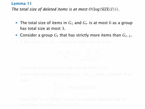
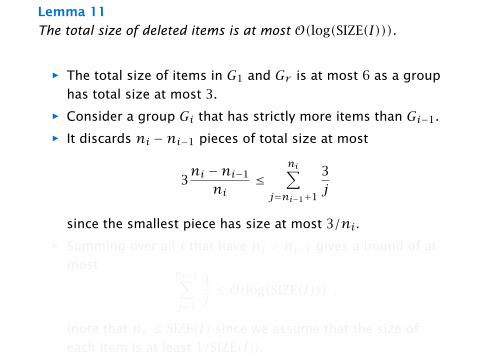
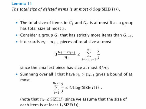
Lemma 11
The total size of deleted items is at most O(log(SIZE(I))).
ñ The total size of items in G1 and Gr is at most 6 as a group
has total size at most 3.
ñ Consider a group Gi that has strictly more items than Gi−1.
ñ It discards ni −ni−1 pieces of total size at most
3ni −ni−1
ni≤
ni∑j=ni−1+1
3j
since the smallest piece has size at most 3/ni.ñ Summing over all i that have ni > ni−1 gives a bound of at
mostnr−1∑j=1
3j≤ O(log(SIZE(I))) .
(note that nr ≤ SIZE(I) since we assume that the size of
each item is at least 1/SIZE(I)).
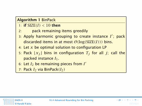
Algorithm 1 BinPack
1: if SIZE(I) < 10 then
2: pack remaining items greedily
3: Apply harmonic grouping to create instance I′; pack
discarded items in at most O(log(SIZE(I))) bins.
4: Let x be optimal solution to configuration LP
5: Pack bxjc bins in configuration Tj for all j; call the
packed instance I1.
6: Let I2 be remaining pieces from I′
7: Pack I2 via BinPack(I2)
EADS II 16.4 Advanced Rounding for Bin Packing
© Harald Räcke 357/521
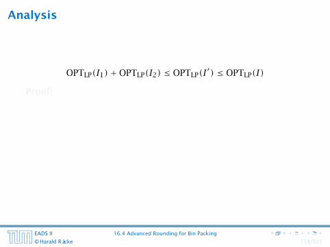
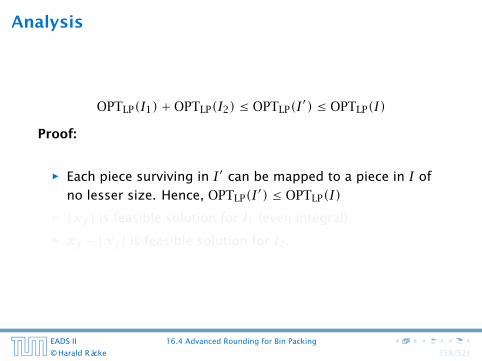
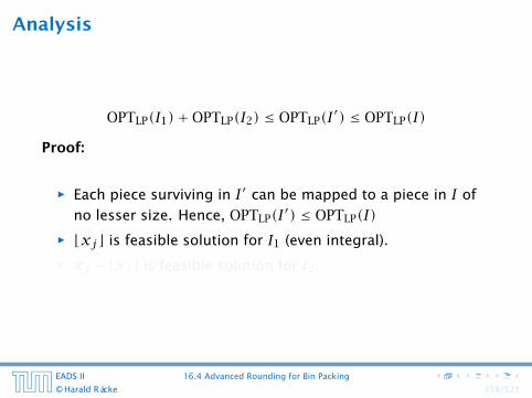
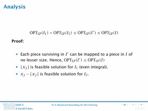
Analysis
OPTLP(I1)+OPTLP(I2) ≤ OPTLP(I′) ≤ OPTLP(I)
Proof:
ñ Each piece surviving in I′ can be mapped to a piece in I of
no lesser size. Hence, OPTLP(I′) ≤ OPTLP(I)ñ bxjc is feasible solution for I1 (even integral).
ñ xj − bxjc is feasible solution for I2.
EADS II 16.4 Advanced Rounding for Bin Packing
© Harald Räcke 358/521
Analysis
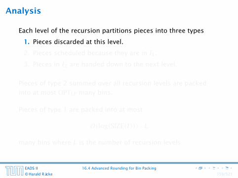
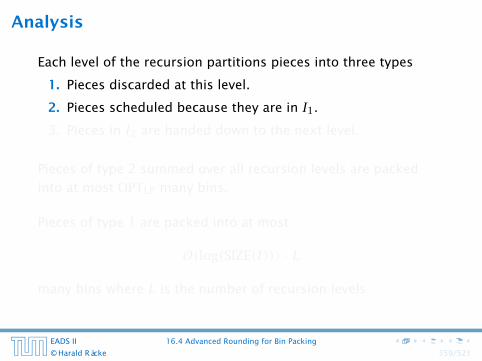
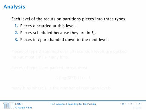
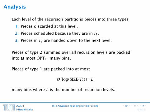
Each level of the recursion partitions pieces into three types
1. Pieces discarded at this level.
2. Pieces scheduled because they are in I1.
3. Pieces in I2 are handed down to the next level.
Pieces of type 2 summed over all recursion levels are packed
into at most OPTLP many bins.
Pieces of type 1 are packed into at most
O(log(SIZE(I))) · L
many bins where L is the number of recursion levels.
EADS II 16.4 Advanced Rounding for Bin Packing
© Harald Räcke 359/521
Analysis
Each level of the recursion partitions pieces into three types
1. Pieces discarded at this level.
2. Pieces scheduled because they are in I1.
3. Pieces in I2 are handed down to the next level.
Pieces of type 2 summed over all recursion levels are packed
into at most OPTLP many bins.
Pieces of type 1 are packed into at most
O(log(SIZE(I))) · L
many bins where L is the number of recursion levels.
EADS II 16.4 Advanced Rounding for Bin Packing
© Harald Räcke 359/521
Analysis
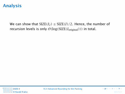
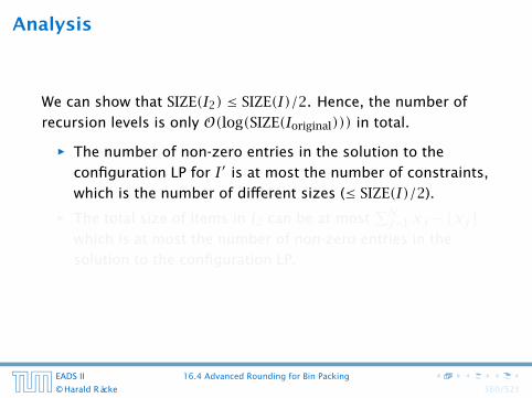
We can show that SIZE(I2) ≤ SIZE(I)/2. Hence, the number of
recursion levels is only O(log(SIZE(Ioriginal))) in total.
ñ The number of non-zero entries in the solution to the
configuration LP for I′ is at most the number of constraints,
which is the number of different sizes (≤ SIZE(I)/2).
ñ The total size of items in I2 can be at most∑Nj=1 xj − bxjc
which is at most the number of non-zero entries in the
solution to the configuration LP.
EADS II 16.4 Advanced Rounding for Bin Packing
© Harald Räcke 360/521
Analysis
We can show that SIZE(I2) ≤ SIZE(I)/2. Hence, the number of
recursion levels is only O(log(SIZE(Ioriginal))) in total.
ñ The number of non-zero entries in the solution to the
configuration LP for I′ is at most the number of constraints,
which is the number of different sizes (≤ SIZE(I)/2).
ñ The total size of items in I2 can be at most∑Nj=1 xj − bxjc
which is at most the number of non-zero entries in the
solution to the configuration LP.
EADS II 16.4 Advanced Rounding for Bin Packing
© Harald Räcke 360/521

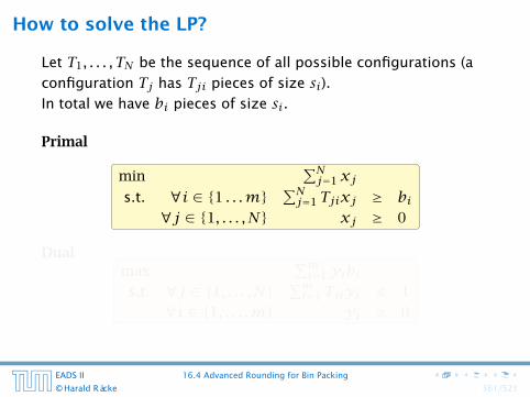
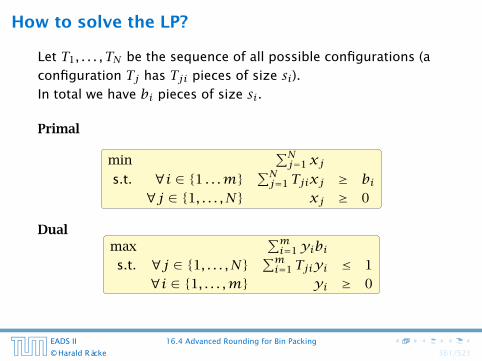
How to solve the LP?
Let T1, . . . , TN be the sequence of all possible configurations (a
configuration Tj has Tji pieces of size si).In total we have bi pieces of size si.
Primal
min∑Nj=1 xj
s.t. ∀i ∈ {1 . . .m}∑Nj=1 Tjixj ≥ bi
∀j ∈ {1, . . . ,N} xj ≥ 0
Dualmax
∑mi=1yibi
s.t. ∀j ∈ {1, . . . ,N}∑mi=1 Tjiyi ≤ 1
∀i ∈ {1, . . . ,m} yi ≥ 0
EADS II 16.4 Advanced Rounding for Bin Packing
© Harald Räcke 361/521

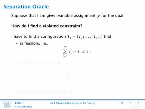
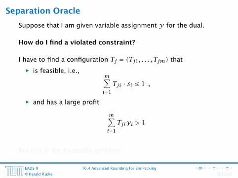
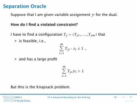
Separation Oracle
Suppose that I am given variable assignment y for the dual.
How do I find a violated constraint?
I have to find a configuration Tj = (Tj1, . . . , Tjm) that
ñ is feasible, i.e.,m∑i=1
Tji · si ≤ 1 ,
ñ and has a large profit
m∑i=1
Tjiyi > 1
But this is the Knapsack problem.
EADS II 16.4 Advanced Rounding for Bin Packing
© Harald Räcke 362/521
Separation Oracle
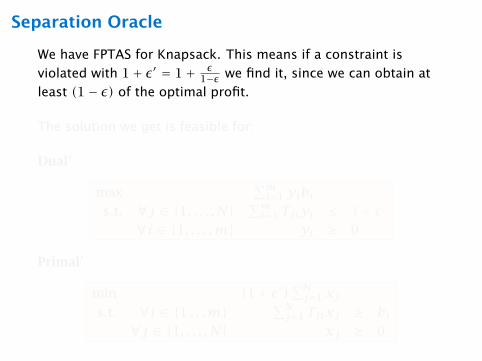
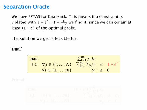
We have FPTAS for Knapsack. This means if a constraint is
violated with 1+ ε′ = 1+ ε1−ε we find it, since we can obtain at
least (1− ε) of the optimal profit.
The solution we get is feasible for:
Dual′
max∑mi=1yibi
s.t. ∀j ∈ {1, . . . ,N}∑mi=1 Tjiyi ≤ 1+ ε′
∀i ∈ {1, . . . ,m} yi ≥ 0
Primal′
min (1+ ε′)∑Nj=1 xj
s.t. ∀i ∈ {1 . . .m}∑Nj=1 Tjixj ≥ bi
∀j ∈ {1, . . . ,N} xj ≥ 0
Separation Oracle
We have FPTAS for Knapsack. This means if a constraint is
violated with 1+ ε′ = 1+ ε1−ε we find it, since we can obtain at
least (1− ε) of the optimal profit.
The solution we get is feasible for:
Dual′
max∑mi=1yibi
s.t. ∀j ∈ {1, . . . ,N}∑mi=1 Tjiyi ≤ 1+ ε′
∀i ∈ {1, . . . ,m} yi ≥ 0
Primal′
min (1+ ε′)∑Nj=1 xj
s.t. ∀i ∈ {1 . . .m}∑Nj=1 Tjixj ≥ bi
∀j ∈ {1, . . . ,N} xj ≥ 0
Separation Oracle
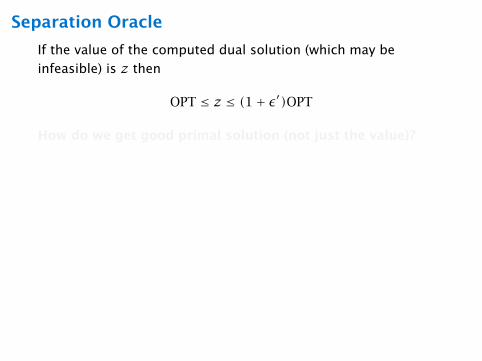
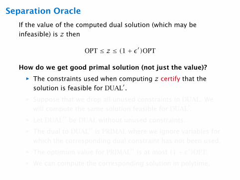
If the value of the computed dual solution (which may be
infeasible) is z then
OPT ≤ z ≤ (1+ ε′)OPT
How do we get good primal solution (not just the value)?
ñ The constraints used when computing z certify that the
solution is feasible for DUAL′.
ñ Suppose that we drop all unused constraints in DUAL. We
will compute the same solution feasible for DUAL′.
ñ Let DUAL′′ be DUAL without unused constraints.
ñ The dual to DUAL′′ is PRIMAL where we ignore variables for
which the corresponding dual constraint has not been used.
ñ The optimum value for PRIMAL′′ is at most (1+ ε′)OPT.
ñ We can compute the corresponding solution in polytime.
Separation Oracle
If the value of the computed dual solution (which may be
infeasible) is z then
OPT ≤ z ≤ (1+ ε′)OPT
How do we get good primal solution (not just the value)?
ñ The constraints used when computing z certify that the
solution is feasible for DUAL′.
ñ Suppose that we drop all unused constraints in DUAL. We
will compute the same solution feasible for DUAL′.
ñ Let DUAL′′ be DUAL without unused constraints.
ñ The dual to DUAL′′ is PRIMAL where we ignore variables for
which the corresponding dual constraint has not been used.
ñ The optimum value for PRIMAL′′ is at most (1+ ε′)OPT.
ñ We can compute the corresponding solution in polytime.
This gives that overall we need at most
(1+ ε′)OPTLP(I)+O(log2(SIZE(I)))
bins.
We can choose ε′ = 1OPT as OPT ≤ #items and since we have a
fully polynomial time approximation scheme (FPTAS) for
knapsack.
EADS II 16.4 Advanced Rounding for Bin Packing
© Harald Räcke 365/521
This gives that overall we need at most
(1+ ε′)OPTLP(I)+O(log2(SIZE(I)))
bins.
We can choose ε′ = 1OPT as OPT ≤ #items and since we have a
fully polynomial time approximation scheme (FPTAS) for
knapsack.
EADS II 16.4 Advanced Rounding for Bin Packing
© Harald Räcke 365/521