16.1. - university of virginiagalileo.phys.virginia.edu/classes/321.jvn.fall02/var... · ·...
TRANSCRIPT

Chapter 16
Variational methods
The calculus of variations originated with attempts to solve Queen Dido'sproblem1, known to mathematicians as the isoperimetric problem: to deter-mine the shape of that closed plane curve of �xed length that encloses themaximum possible area.
The next major development was the brachistochrone problem: to �nd thecurve of a thin wire joining two points at di�erent elevations, down whicha bead slides without friction, in minimum time. According to lore, thisproblem was �rst posed by Galileo; the Swiss mathematician Jakob Bernoullisubsequently (in the late 17th Century) o�ered a reward for its solution. The�rst to solve it was apparently Isaac Newton, who submitted his solutionanonymously. Bernoulli was not fooled, however, remarking \One knowsthe lion by his claw."
Problems of extrema remain a rich and diÆcult area of modern mathematics.Plateau's problem|to �nd the surface of minimum area that spans a generalclosed curve in space|is unsolved to this day2.
The possibility of expressing physical principles in a mathematical form, in
1According to legend, Dido, in return for a service to a North African chieftain, wasgiven as much land as she could enclose within a bull's hide. She cleverly �rst cut the hideinto thongs, tied them together to make a long string, and enclosed with them a circularplot of ground, upon which she founded the city of Cathage.
2An �thestic aspect of Plateau's problem arises from the fact that soap �lms on bentwire frames tend to minimize the energy of surface tension, thereby minimizing their area.
429

430 CHAPTER 16. VARIATIONAL METHODS
which the desired result makes some quantity that depends on it an ex-tremum, has turned out to be of enormous importance. It is the basis ofHamilton's Principle in mechanics, has led subsequently to the path integralformulation of quantum mechanics, and is also the basis of quantum �eldtheory, not to mention string theory. The practical applications of varia-tional methods are legion, in �elds ranging from structural engineering toeconomics and �nance. This chapter will touch on the basic ideas and somerepresentative applications.
16.1 Classical variational calculus
In di�erential calculus we often make use of the property that the derivativeof a function (of one or several variables) vanishes at a (local) minimumor maximum to locate such extremal points. As we have seen in Chapter9, we can think of functions|especially continuous ones|as vectors in anabstract space. If this space is a separable Hilbert space such as L2 wecan think of the function as a denumerable set of independent variables3.In that case a functional F (ffg) that depends on the function f(x) is thegeneralization, from an ordinary function of several variables, to a functionof in�nitely many variables.
16.1.1 Functionals
Here are some speci�c examples of functionals:
1. Suppose a curve in the plane is represented by the vector ~r = (x; y = f(x));then the length of the curve is
` =
Z b
adx
q1 + (f 0(x))2
and the area enclosed between it and the x-axis is
A =
Z b
af(x) dx :
3: : :for example the coeÆcients in an expansion of f(x) in a complete set of orthonormalfunctions �k(x).

16.1. CLASSICAL VARIATIONAL CALCULUS 431
2. If an arbitrary curve f(x) represents a stationary uniform chain ofmass � per unit length, then its (potential) energy is
V = �g
Z b
adx f(x)
q1 + (f 0(x))2 :
3. If the curve f(x) represents a sti� wire in the vertical plane (x hori-zontal, y vertical), along which a bead can slide without friction underthe in uence of gravity, then the time the bead takes to slide downthe wire is
T =
Z b
a
ds(x)
v(x)�Z b
adx
s1 + (f 0(x))2
2gf(x)
4. If
~r(�) =
0B@ x(�)y(�)z(�)
1CA
represents the parametric curve of a light ray in a medium of variablerefractive index n (~r), then
T =1
c
Z �2
�1
n (~r (�))q_x2 + _y2 + _z2 d�
is the time for the light to go from ~r (�1) to ~r (�2), where _x = dx/d� ,etc.
5. The energy of a thin beam of uniform density � per unit length, witha central load W at the midway point is
E (f�g) =LZ0
24Y I
2
d2�
dz2
!2
+ �g� (z) +WÆ (z � L/2) � (z)
35 dz ;
where Y is Young's modulus and I the \areal moment of inertia".

432 CHAPTER 16. VARIATIONAL METHODS
16.1.2 The Euler-Lagrange equation
The central problem of the calculus of variations is to �nd extrema of func-tionals. The basic idea is this: replace the unknown function f in thefunctional F ffg by f + �, where �(x) is a \small" function. The variationof F under this change is
ÆF = F (ff + �g)�F (ffg) ;
if f is the function that makes the functional extremal, the variation mustvanish, to �rst order in �. To make this more explicit, consider a functionalthat depends only on f(x), f 0(x) and explicitly on x:
F (ffg) =Z b
a��f(x); f 0(x); x
�dx : (16.1)
Clearly,
ÆF (ffg) =
=
Z b
a
���f(x) + �(x); f 0(x) + �0(x); x
�� ��f(x); f 0(x); x
��dx
=
Z b
a
�@�
@f� +
@�
@f 0�0 + : : :
�dx
We then set the terms linear in � to zero. The diÆculty we now face is thatwhile we imagine we know the \small" deviation �, we know nothing aboutits derivative. So the idea is to re-express the term containing (�)0 so we getrid of the derivative. This can be accomplished using integration by parts:
Z b
a
@�
@f 0�0(x) dx =
Z b
a
d
dx
�@�
@f 0�
�dx�
Z b
a�d
dx
�@�
@f 0
�dx
=
�@�
@f 0�
�����ba
�Z b
a�d
dx
�@�
@f 0
�dx :

16.1. CLASSICAL VARIATIONAL CALCULUS 433
We now note that in most cases we want to specify the values f(a) and f(b).For example, in the brachistochrone problem the end points (x; y) are �xed.The function �(x) must therefore vanish at the ends of the interval, so theperfect derivative term vanishes:
�@�
@f 0�
�����b
a
= 0
and we can write, to �rst order in �,
ÆF =
Z b
a
�@�
@f� d
dx
�@�
@f 0
��� (x) dx = 0 : (16.2)
Now the variation �(x) can be any function that vanishes at x = a andx = b. Hence we may take it to be proportional to successive members of acomplete orthonormal system. The extremal condition then amounts to thestatement that the contents of the square bracket in Eq. 16.2 is orthogonalto every member of a complete set. This means that the bracketed functionitself must vanish for all x 2 [a; b], except possibly on a set of Lebesguemeasure zero. That is, we have found
@�
@f� d
dx
�@�
@f 0
�= 0 : (16.3)
Equation 16.3 is known as the Euler-Lagrange equation.
. . . . . . . . . . . . . . . . . . . . . . . . . . . . . . . . . . . . . . . . . . . . . . . . . . . . . . . . . . . . . . . . . . . . . . . . . .
Exercise 16.1
If we approximate the function f(x) by the �rst N terms of its expansion ina complete orthonormal set f�kg,
f (x) =NXk=1
fk�k (x) ;
we may think of the functionalF as a function of a �nite number of variables,fk. With F de�ned as in Eq. 16.1, show that the condition for F to have

434 CHAPTER 16. VARIATIONAL METHODS
an extremum:
@F
@fk= 0; k = 1; : : : ; N
can be put in the form of the Euler-Lagrange equation, as long as
�N (x) =NXk=1
Æfk�k (x)
vanishes at the endpoints of the interval.
. . . . . . . . . . . . . . . . . . . . . . . . . . . . . . . . . . . . . . . . . . . . . . . . . . . . . . . . . . . . . . . . . . . . . . . . . .
16.1.3 Applications
Let us begin with the brachistochrone problem. A bead slides frictionlesslyon a wire that is bent into a plane curve, in the x�z plane, and falls from aninitial point (a; za) to a lower point (b; zb). The time of the fall is therefore
T =
Z b
a
ds(x)
v(x)�Z b
adx
s1 + (z0(x))2
2g z(x):
The function � is
��z; z0
�=
s1 + (z0(x))2
z(x)
(the factor 2g is immaterial) and the Euler-Lagrange equation becomes
@�
@z� d
dx
�@�
@z0
�
� �1
2
s1 + (z0(x))2
z3(x)� d
dx
0BB@ z0(x)r
z(x)h1 + (z0(x))2
i1CCA = 0

16.1. CLASSICAL VARIATIONAL CALCULUS 435
This leads to an impressively ugly second-order nonlinear di�erential equa-tion to solve, so it is best to employ a trick. We turn the problem on itsside, so to speak, and take z for the variable of integration. Then letting_x = dx/dz we have
Æ
Z zb
za
dz
s1 + _x2
z= 0
or (since there is no explicit dependence on x)
d
dz
0@ _x
1 + _x2
s1 + _x2
z
1A = 0 :
This can be integrated immediately, and squared, to give the �rst-orderequation
1
z� _x2
1 + _x2= A2
which leads to the separable form
dx = �dzs
A2z
1�A2z:
We want the � sign because on physical grounds the altitude z(x) mustdecrease monotonically with x. The solution is the equation of a cycloid,
A2x+B =qA2z (1�A2z)� sin�1
pA2z ;
where the constants A2 and B must be adjusted to match the initial and�nal conditions.
As a second application, let us solve Dido's problem. We express the curveparametrically (in Cartesian coordinates) in terms of an angle �:
A =1
2
Z 2�
0d�hx2 (�) + y2 (�)
i

436 CHAPTER 16. VARIATIONAL METHODS
` =
Z 2�
0d�q_x2 (�) + _y2 (�)
as shown below
where
_x = dxd�; _y = dy
d�:
We want to maximize the area A while keeping the perimeter ` �xed4; thisis an example of a constrained variational problem. We employ the samedevice used when �nding the extremum of a function of a �nite numberof variables, subject to constraints|namely a Lagrange multiplier for eachconstraint. We therefore want to set
Æ (�A+ `) = 0
which leads to the Euler-Lagrange equations (there are two equations, onefor each function x(�) and y(�))
�x+_y
( _x2 + _y2)3/2( _x �y � _y �x) = 0
4: : :or minimize ` while keeping A constant.
16.1. CLASSICAL VARIATIONAL CALCULUS 437
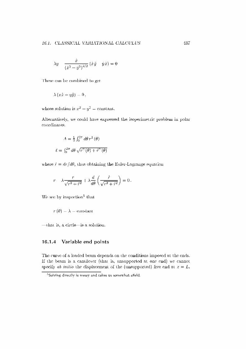
�y � _x
( _x2 + _y2)3/2( _x �y � _y �x) = 0
These can be combined to get
� (x _x+ y _y) = 0 ;
whose solution is x2 + y2 = constant.
Alternatively, we could have expressed the isoperimetric problem in polarcoordinates,
A = 12
R 2�0 d� r2 (�)
` =R 2�0 d�
pr2 (�) + _r2 (�)
where _r = dr/d�, thus obtaining the Euler-Lagrange equation
r � �rp
r2 + _r2+ �
d
d�
�_rp
r2 + _r2
�= 0 :
We see by inspection5 that
r (�) = � = constant
|that is, a circle|is a solution.
16.1.4 Variable end points
The curve of a loaded beam depends on the conditions imposed at the ends.If the beam is a cantilever (that is, unsupported at one end) we cannotspecify ab initio the displacement of the (unsupported) free end at z = L.
5Solving directly is messy and takes us somewhat a�eld.

438 CHAPTER 16. VARIATIONAL METHODS
All we can say is that �(0) = �0(0) = 0 (because obviously, the supportedend must be clamped or it cannot remain in static equilibrium). If we varythe energy (here we consider the case with a weight hung on the free end ofthe beam) to �nd its minimum, we obtain
Æ
Z L
0
�Y I
2
��00�2+ �g� +WÆ (z � L+ ") �
�= 0
or, with f(z) = �g� +WÆ (z � L+ "),
Z L
0
"Y I
d4�
dz4+ f(z)
#�+
Y I
d2�
dz2�0!�����
L
0
� Y I
d3�
dz3�
!�����L
0
= 0 :
(Note that we get around any problems with the delta function by hangingthe weight a distance " in from the end. We can let " ! 0 after we aredone.) Because the function �(z) is arbitrary, the Euler-Lagrange equation
Y Id4�
dz4+ f(z) = 0
is still satis�ed. However, we now also have the end-point contributions
Y I
d2�
dz2�0
!�����L
0
� Y I
d3�
dz3�
!�����L
0
that must vanish as well. The conditions at the clamped end require
�(0) = �0(0) = 0
so we deduce the subsidiary conditions
d2�
dz2
�����z=L
=d3�
dz3
�����z=L
= 0 :

16.1. CLASSICAL VARIATIONAL CALCULUS 439
To solve this problem we simply integrate:
d3�
dz3
!�����z
0
= � 1
Y I
Z z
0d� f (�) = � �g
Y Iz � W
Y I� (z � L+ ")
or
d3�
dz3= A� �g
Y Iz � W
Y I� (z � L+ ") :
Integrating again,
d2�
dz2= B +Az � �g
2Y Iz2 � W
Y I(z � L+ ") � (z � L+ ")
and again,
d�
dz=
�d�
dz
����z=0
� 0
�+Bz +
A
2z2 � �g
6Y Iz3 � W
2Y I(z � L+ ")2 � (z � L+ ")
and a �nal time yields
� = (�(0) � 0) +B
2z2 +
A
6z3 � �g
24Y Iz4 � W
6Y I(z � L+ ")3 � (z � L+ ") :
The two non-vanishing constants of integration, A;B, are determined fromthe end-point conditions at z = L:
�00(L) = 0 ) B +AL� �g2Y IL
2 = 0
�000(L) = 0 ) A� �gY IL� W
Y I= 0
leading to
� (z) = �1
2
�gL2
2Y I+WL
Y I
!z2 +
1
6
��gL
Y I+W
Y I
�z3 � �g
Y Iz4 :

440 CHAPTER 16. VARIATIONAL METHODS
. . . . . . . . . . . . . . . . . . . . . . . . . . . . . . . . . . . . . . . . . . . . . . . . . . . . . . . . . . . . . . . . . . . . . . . . . .
Exercise 16.2
Find the curve of a uniform chain of mass � per unit length, hanging fromtwo level supports a distance L apart, by minimizing its potential energy
V = �g
Z b
adx y(x)
q1 + (y0(x))2
subject to a suitable constraint.
. . . . . . . . . . . . . . . . . . . . . . . . . . . . . . . . . . . . . . . . . . . . . . . . . . . . . . . . . . . . . . . . . . . . . . . . . .
Exercise 16.3
Find the curve of a uniform thin beam of mass � per unit length, loadedwith a point weight W halfway between the level end-supports, for the twocases:
a) the ends are clamped to be horizontal (that is, both the displacement�, and its �rst derivative, d�/dz vanish at both ends);
b) the ends simply rest on the supports (that is, the displacement � van-ishes at the ends, but its derivative is unconstrained there).
. . . . . . . . . . . . . . . . . . . . . . . . . . . . . . . . . . . . . . . . . . . . . . . . . . . . . . . . . . . . . . . . . . . . . . . . . .
Exercise 16.4
In x16.1.1, the fourth example is Fermat's Principle of Least Time. Considertwo cases:
a) Light travels from one medium of uniform refractive index n1 across aplane interface to another medium of (uniform) index n2. Show thatthe ray obeys Snell's Law.
b) The index has the form n(x; y; z) = 1+�z. What is the equation of thecurve traversed by a light ray, taking x as the parameter representingthe curve|that is, what are y(x) and z(x)? (This is the explanationof the mirage.)
. . . . . . . . . . . . . . . . . . . . . . . . . . . . . . . . . . . . . . . . . . . . . . . . . . . . . . . . . . . . . . . . . . . . . . . . . .

16.2. HAMILTON'S PRINCIPLE 441
16.2 Hamilton's principle
D'Alembert's principle of virtual work [?] allows us to derive the equationsof motion for mechanical systems, subject to holonomic constraints, directlyfrom Newton's Second Law of motion,
d~p
dt= ~F :
For each generalized coordinate q(t) we �nd an equation of the form
@L
@q� d
dt
�@L
@ _q
�= 0 : (16.4)
We immediately recognize this as the Euler-Lagrange equation, where L isthe Lagrangian of the system, expressed in terms of kinetic energy T andpotential energy V
L = T � V :
Sir William Rowan Hamilton noticed that Eq. 16.4 could be expressed as avariational problem,
Æ
Z t2
t1
dtL (q; _q; t) = 0 ; (16.5)
now called variously Hamilton's Principle, or the Principle of Least Action6,since Eq. 16.4 is just the corresponding Euler-Lagrange equation for thefunction q(t) that makes the functional in Eq. 16.5 an extremum.
. . . . . . . . . . . . . . . . . . . . . . . . . . . . . . . . . . . . . . . . . . . . . . . . . . . . . . . . . . . . . . . . . . . . . . . . . .
Exercise 16.5
The Lagrangian of a pendulum, consisting of a bob of mass m and negligiblephysical extension on the end of a massless rigid rod of length `, suspended
6The latter name derives from the fact that the time-integral of the Lagrangian inEq. 16.5 is called the action.

442 CHAPTER 16. VARIATIONAL METHODS
below a �xed pivot is
L =m
2
�_x2 + _y2
��mgy
where x and y are the position coordinates of the bob, and _x and _y respec-tively the components of its velocity.
a) Express the Lagrangian in terms of a single generalized coordinate,the angle � the rod makes with the vertical.
b) Derive the equation of motion for �(t).
c) Reduce this equation to quadrature (that is, express the answer as anintegral).
. . . . . . . . . . . . . . . . . . . . . . . . . . . . . . . . . . . . . . . . . . . . . . . . . . . . . . . . . . . . . . . . . . . . . . . . . .
16.3 The role of symmetry
Principle of Least Action is important in theoretical physics because it pro-vides a way to incorporate the fundamental symmetries of a system ab initio,thereby restricting the possible forms that the Lagrangian can take. Con-sider, for example, a non-interacting particle in three dimensions. Trans-lation invariance in space and time implies the Lagrangian cannot dependeither on position ~x or on the time, t. Hence it can depend only on thevelocity,
~v =d~x
dt:
Rotation invariance implies the Lagrangian must be a scalar, i.e. a functionof ~v � ~v. The simplest such function is
L =1
2m~v � ~v ;

16.3. THE ROLE OF SYMMETRY 443
which we see is the usual non-relativistic kinetic energy.
We could have determined the form of the Lagrangian, up to the factor m/2,by imposing the symmetry of Galilean invariance. According to Galileo, ifthe velocity of a particle in frame S is ~v, then in frame S 0 moving withvelocity ~V relative to the �rst, the velocity is
~v0 = ~v � ~V ;
and the time di�erential is
dt0 = dt :
Since the Lagrangian is a general function of ~v2, we have in system S 0,
A0 =
Z t2
t1
dtL
��~v � ~V
�2�
We want A0 to be reducible to A plus, at most, a constant. Suppose ~V issmall|then we can expand in Taylor's series to �nd
A0 �Z t2
t1
dt
�L�~v2�� 2~v � ~V @L
@ (~v2)+ : : :
�:
Now, in order for the term
�A0 = �2~V �Z t2
t1
dt
�~v@L
@ (~v2)
�
to be a constant|that is, independent of the path taken by the particle7|the integrand must be a perfect di�erential with respect to time. Since
7This condition must be satis�ed in order that varying the term �A0 not a�ect thedynamics.

444 CHAPTER 16. VARIATIONAL METHODS
~v is already a perfect di�erential, namely d~x/dt, the only way the entireintegrand can be a perfect di�erential is if
@L
@ (~v2)= constant ;
that is, if L / ~v2. In plain terms, the only possible Galilean-invariantLagrangian that describes a non-interacting particle is
L =1
2m~v2 :
Suppose we wanted to impose Lorentz invariance, rather than Galilean in-variance, as the fundamental symmetry. As Einstein showed, the correctformula for addition of velocities is, for small ~V (but large ~v),
~v0 � ~v � ~V
1� ~v � ~V.c2:
We must also correct the time: in the moving frame we have, under thesame conditions,
dt0 � dt�1� ~v � ~V
.c2�:
Hence
A0 � A� ~V �Z t2
t1
dt~v
�L
c2+ 2
�1� ~v2
.c2� @L
@ (~v2)
�;
the condition that the term linear in ~V be independent of path yields therelation
L
c2+ 2
�1� ~v2
.c2� @L
@ (~v2)= � = constant ;

16.4. VARIATIONAL PROBLEMS IN CONTINUOUS SYSTEMS 445
whose solution is
L = �c2 + �
r1� ~v2
.c2 :
To make contact with the nonrelativistic result for small ~v we choose � =m,� = �mc2; thus the unique (up to an additive constant that contributesnothing to the dynamics) Lagrangian is
L = mc2 �mc2r1� ~v2
.c2 :
It is perhaps worth pointing out that
dt
r1� ~v2
.c2 � d� ;
where the di�erential d� of the \proper time" is a manifestly Lorentz-invariant quantity, so the integral
Rd� is also manifestly Lorentz-invariant.
16.4 Variational problems in continuous systems
The equation of motion of a vibrating stretched string is
T@2
@x2� �
@2
@t2= 0 (16.6)
where x is the coordinate along the string, (x; t) is the instantaneous dis-placement of the piece of string between x and x + dx in the directionperpendicular to the string, T is the string tension, and �(x) the mass perunit length. If we look at the string as composed of masses �(x)�x con-nected by massless segments of tension T , and if we add up the kinetic andpotential energies of the masses, we get a Lagrangian
L =1
2
Xxk=k�x
�� (xk)�x
�_ (xk)
�2 � T
�x( (xk+1)� (xk))
2�

446 CHAPTER 16. VARIATIONAL METHODS
!�x!0
1
2
Z `
0dx
"� (x)
�@
@t
�2� T
�@
@x
�2#:
The action is therefore
A =1
2
Zdt
Zdx
"� (x)
�@
@t
�2� T
�@
@x
�2#
and we can apply Hamilton's principle as before. Imagine the string isclamped at the ends; then (0; t) = (`; t) = 0, hence the small variation�(x; t) also vanishes at the supports. The result is that (assuming � alsovanishes at the beginning and end of the time interval in the action)
ÆA =
Zdt
Zdx
"T@2
@x2� �
@2
@t2
#� (x; t) = 0
which, because of the generality of �(x; t), gives us the wave equation 16.6.
The energy (Hamiltonian) of the system becomes
H =1
2
Z `
0dx
"� (x)
�@
@t
�2+ T
�@
@x
�2#(16.7)
where we have made the contact transformation8 that is the continuumequivalent of
H = _q@L
@ _q� L :
Note that the Hamiltonian, Eq. 16.7, is manifestly real and positive.
Suppose we consider sinusoidal vibrations,
(x; t) = cos (!t)' (x) :
8see, e.g. , Goldstein, Classical Mechanics.

16.4. VARIATIONAL PROBLEMS IN CONTINUOUS SYSTEMS 447
The action then becomes
A =1
2
Z t2
t1
dt
Z `
0dx
"!2� (x)'2 sin2(!t)� T
�d'
dx
�2cos2(!t)
#;
which, for time intervals � 2�!�1, has the limit
!t2�t1
1
4
Z `
0dx
"!2� (x)'2 � T
�d'
dx
�2#:
The Principle of Least Action is then equivalent to the constrained extremumproblem
Æ
Z `
0dx
"T
�d'
dx
�2� �� (x) (' (x))2
#= 0
|that is, extremizing the string tension energy while keeping the (weighted)normalization integral
N =
Z `
0dx� (x)'2(x)
�xed. The Lagrange multiplier � is just !2 in the resulting eigenvalue equa-tion
�d2'
dx2= !2
� (x)
T' (x) : (16.8)
If the linear mass-density is uniform , � = constant, Eq. 16.8 is the equivalentof the time-independent Schr�odinger equation for a particle con�ned in aone-dimensional box. This suggests that we might represent all the linearpartial di�erential equations of mathematical physics as appropriate actionprinciples, and that seems to be so.

448 CHAPTER 16. VARIATIONAL METHODS
16.5 Bilinear functionals
We saw in Chapter 11 that the matrix elements h'jH j i of linear operatorsin Hilbert space could be regarded as bilinear functionals of the functions 'and . The eigenvalue equation
H = �
may therefore be obtained by varying with respect to 'y subject to the con-straint h' j i = constant. The relation between the variational calculus andlinear eigenvalue problems leads to some useful approximation techniques.
16.5.1 Rayleigh-Ritz upper bound
For example, suppose the operator H is hermitian9 on some Hilbert spaceH: then its eigenfunctions form a complete orthogonal system f'kg10 withcorresponding (real) eigenvalues hk. We may then express any diagonalmatrix element of H as
h jH j i =1Xk=0
jckj2 hk ;
where
(x) =1Xk=0
h'k j i'k (x) =1Xk=0
ck'k (x) :
Now consider the ratio
h jH j ih j i �
1Pk=0
jckj2 hk1Pk=0
jckj2; (16.9)
9: : : or better yet, essentially self-adjoint.

16.5. BILINEAR FUNCTIONALS 449
since jckj2 > 0, the right hand side of Eq. 16.9 can be minimized by replacingall the hk by the smallest eigenvalue. That is, for any
hmin �
1Pk=0
jckj2 hk1Pk=0
jckj2� h jH j i
h j idf= �h :
This fact leads to the Rayleigh-Ritz variational method for estimating thelowest eigenvalue of the operator H: we choose a function that containsundetermined parameters, compute the left side of Eq. 16.9, obtaining afunction of those parameters, then minimize that function, obtaining a �niteset of algebraic equations to solve. By this means the ground state energy(and hence the electron removal energy) of the helium atom was calculatedto great precision, historically providing enormous con�dence in the newquantum mechanics.
. . . . . . . . . . . . . . . . . . . . . . . . . . . . . . . . . . . . . . . . . . . . . . . . . . . . . . . . . . . . . . . . . . . . . . . . . .
Exercise 16.6
Find an upper bound to the ground state energy of a one-dimensionalquantum-mechanical harmonic oscillator whose Hamiltonian is
H = � �h2
2m
d2
dx2+1
2m2x2 ;
using a trial function that is the ground state of a particle in a 1-dimensionalbox of width L. (That is, take L for your variational parameter.) Make surethe wave function is symmetric about x = 0.
. . . . . . . . . . . . . . . . . . . . . . . . . . . . . . . . . . . . . . . . . . . . . . . . . . . . . . . . . . . . . . . . . . . . . . . . . .
Exercise 16.7
Compute an upper bound to the ground state energy of the hydrogenic atomin three dimensions, with Hamiltonian
H = � �h2
2mr2 � Ze2
r;

450 CHAPTER 16. VARIATIONAL METHODS
using a trial wave function of the form
(~r) = e��r2
:
. . . . . . . . . . . . . . . . . . . . . . . . . . . . . . . . . . . . . . . . . . . . . . . . . . . . . . . . . . . . . . . . . . . . . . . . . .
16.5.2 Lower bounds
We may evaluate the ratio10
K (�; f g) =�H � �h
� �� (H � �)
�h j i � hH j H i
h j i � �h2df=�� �h2
for any � and any . We then may expand in eigenfunctions of H toobtain
K (�; f g) = �� �h2 =
1Pk=0
jckj2�hn � �h
�(hn � �)
1Pk=0
jckj2:
There are two ways we might use this relation:
1. let � = �h and suppose we know that
�hmin � �h
�2 � �hn � �h�2 8n ;
clearly, then,
�� �h2 =
1Pk=0
jckj2�hn � �h
�21Pk=0
jckj2� �hmin � �h
�2 � 0 ;
10The methods in this subsection come from Goertzel and Tralli, Some Mathematical
Methods of Physics.

16.5. BILINEAR FUNCTIONALS 451
or
�h�p�� �h2 � hmin � �h+
p�� �h2 :
(For this bound to have the correct ordering and signs, either H mustbe positive, or else if hmin < 0, the Rayleigh-Ritz upper bound �h mustalso be negative.)
Example:Let us consider the vibrating string of unit length. Thenwe can obtain an upper bound on the lowest eigenvalue,hmin, (which we know is �2) of �D2 � �d2Ædx2 using adi�erentiable function (x) which vanishes at x = 0 and atx = 1. Such a function is x(1� x). Then
�h =
R 10 dx
hddx(x (1� x))
i2R 10 dx [x (1� x)]2
= 10 > �2 :
We evaluate the lower bound next:
� =
R 10 dx
hd2
dx2(x (1� x))
i2R 10 dx [x (1� x)]2
= 120
or, combining the two bounds,
10�p120 � 100 � hmin � �h = 10 :
Admittedly 10 � p20 = 5:527 : : : is not a very close lower
bound to �2, but it is de�nitely a lower bound. With moreinformation we can do better, as we see below.
2. Suppose we have approximate knowledge of the second eigenvalue, h1(we suppose the eigenvalues are ordered, hmin � h0 � h1 � h2 : : :).Then if we know that h0 � �h � h1, choose
� = h0 + h1 � �h ;
giving
�� �h2 =
1Pk=0
jckj2�hn � �h
� �hn + �h� h0 � h1
�1Pk=0
jckj2:
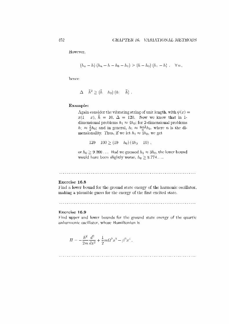
452 CHAPTER 16. VARIATIONAL METHODS
However,
�hn � �h
� �hn + �h� h0 � h1
� � ��h� h0� �h1 � �h
�; 8n ;
hence
�� �h2 � ��h� h0� �h1 � �h
�:
Example:
Again consider the vibrating string of unit length, with (x) =x(1 � x), �h = 10, � = 120. Now we know that in 1-dimensional problems h1 � 4h0; for 2-dimensional problemsh1 � 5
2h0; and in general, h1 � n+3nh0, where n is the di-
mensionality. Thus, if we let h1 � 4h0, we get
120� 100 � (10� h0) (4h0 � 10) ;
or h0 � 9:260 : : :. Had we guessed h1 � 3h0, the lower boundwould have been slightly worse, h0 � 8:774 : : :.
. . . . . . . . . . . . . . . . . . . . . . . . . . . . . . . . . . . . . . . . . . . . . . . . . . . . . . . . . . . . . . . . . . . . . . . . . .
Exercise 16.8
Find a lower bound for the ground state energy of the harmonic oscillator,making a plausible guess for the energy of the �rst excited state.
. . . . . . . . . . . . . . . . . . . . . . . . . . . . . . . . . . . . . . . . . . . . . . . . . . . . . . . . . . . . . . . . . . . . . . . . . .
Exercise 16.9
Find upper and lower bounds for the ground state energy of the quarticanharmonic oscillator, whose Hamiltonian is
H = � �h2
2m
d2
dx2+1
2m2x2 + �2x4 :
. . . . . . . . . . . . . . . . . . . . . . . . . . . . . . . . . . . . . . . . . . . . . . . . . . . . . . . . . . . . . . . . . . . . . . . . . .

16.5. BILINEAR FUNCTIONALS 453
16.5.3 Bounds for positive operators
A positive operator A � 0 is a Hermitian operator for which h�jA j�i � 0for any vector j�i in the Hilbert space. We say an operator A � C if bothare Hermitian and
h�j (A� C) j�i � 0 :
Using the trial vector
j�i = ji �NXn=1
cn j'ni
where the f'ngN1 are any set of N vectors in H and is an arbitrary vector,we see that
h�jA j�i = h jA j i �NXn=1
(cn hjA j'ni+ c�n h'njA ji)
+Xm;n
c�mcn h'mjA j'ni
� 0 :
Treating the c�n as variational parameters we may minimize and evaluate theexpression for the minimizing values, to �nd
h�jA j�imin = h jA j i �Xm;n
h jA j'miBmn h'njA ji � 0 ;
where Bmn is the inverse of the N � N matrix h'mjA j'ni. Since isarbitrary, in operator terms we have found an operator that is a lower boundfor A:
A �Xm;n
A j'miBmn h'njA : (16.10)

454 CHAPTER 16. VARIATIONAL METHODS
The virtue of the bound Eq. 16.10 is that by increasing the number offunctions in the set f'ngN1 we can increase the lower-bounding operatorand thereby improve|say|the lower bound on an eigenvalue.
. . . . . . . . . . . . . . . . . . . . . . . . . . . . . . . . . . . . . . . . . . . . . . . . . . . . . . . . . . . . . . . . . . . . . . . . . .
Exercise 16.10
The electron-electron interaction in the helium atom is manifestly positive,since
h jV ji = e2Zd3r1
Zd3r2
j(~r1; ~r2)j2j~r1 � ~r2j
� 4�e2Zd3R
Zd3q
���~ �~R; ~q����2q2
where
~�~R; ~q
�=
Zd3r
�~R+
1
2~r; ~R� 1
2~r
�ei~q�~r :
Therefore it is possible to bound this term below by an operator of �nite rankN , as in Eq. 16.10, and thereby obtain a series of (increasing) lower boundsto the ground state energy of helium. Choose two suitable trial functionsand thereby obtain a rank-2 lower bound for the ground state energy of He.
. . . . . . . . . . . . . . . . . . . . . . . . . . . . . . . . . . . . . . . . . . . . . . . . . . . . . . . . . . . . . . . . . . . . . . . . . .
16.6 Feynman-Hellman theorem
Suppose a Hermitian operator H(�) depends on a parameter �. Then, natu-rally, all the eigenvalues, hn(�), and eigenvectors, j'n(�)i, will be functionsof � as well. We may express hn(�) as
hn (�) =h'n (�)jH (�) j'n (�)ih'n (�) j 'n (�)i ;
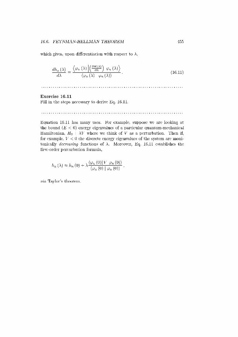
16.6. FEYNMAN-HELLMAN THEOREM 455
which gives, upon di�erentiation with respect to �,
dhn (�)
d��D'n (�)
����@H(�)@�
����'n (�)Eh'n (�) j 'n (�)i : (16.11)
. . . . . . . . . . . . . . . . . . . . . . . . . . . . . . . . . . . . . . . . . . . . . . . . . . . . . . . . . . . . . . . . . . . . . . . . . .
Exercise 16.11
Fill in the steps necessary to derive Eq. 16.11.
. . . . . . . . . . . . . . . . . . . . . . . . . . . . . . . . . . . . . . . . . . . . . . . . . . . . . . . . . . . . . . . . . . . . . . . . . .
Equation 16.11 has many uses. For example, suppose we are looking atthe bound (E < 0) energy eigenvalues of a particular quantum-mechanicalHamiltonian, H0 + �V where we think of V as a perturbation. Then if,for example, V < 0 the discrete energy eigenvalues of the system are moni-tonically decreasing functions of �. Moreover, Eq. 16.11 establishes the�rst-order perturbation formula,
hn (�) � hn (0) + �h'n (0)j V j'n (0)ih'n (0) j 'n (0)i ;
via Taylor's theorem.