16377544 ims dbdc workshop
TRANSCRIPT
IMS DB/DC
Workshop
Design of hierarchical DBs or
A basic presentation about IMS DB/DC…
Presented by
Dipl. Ing. Werner Hoffmann EMAIL: [email protected] or
2007

1
Date: 21.06.2007 IMS_DB_01.ppt Page: 1
IBM Mainframe
IMS DB/DC
Workshop
Design of hierarchical Design of hierarchical DBsDBsoror
A basic presentation about IMS DB/DCA basic presentation about IMS DB/DC……June 2007 June 2007 –– 1st Version1st Version
presented bypresented by
Dipl. Dipl. IngIng. Werner Hoffmann. Werner Hoffmann
EMAIL: EMAIL: pwhoffmann @ tpwhoffmann @ t--online.deonline.de
A member of IEEE and ACM
Mainframe
Please see the notes pages for additional comments. Please see the notes pages for additional comments.
Welcome to the workshop called “IMS DB/DC".
2
IMS_DB Page: 2Date: 21.06.2007
AgendaAgenda
I - Overview Workshop Sessions
II - IMS Overview
III - IMS Hierarchical Database Model
1: Initial Session
2: Basics
3: Hierarchical Access Methods
4: Logical Relationships/ Logical Databases
5: Indexed Databases
6: Data Sharing Issues
7: Implementing IMS DatabasesIV - IMS Transaction Manager – Basics
V - IMS Database Design
VI - IMS DB Implementation (DB Admin.)
…
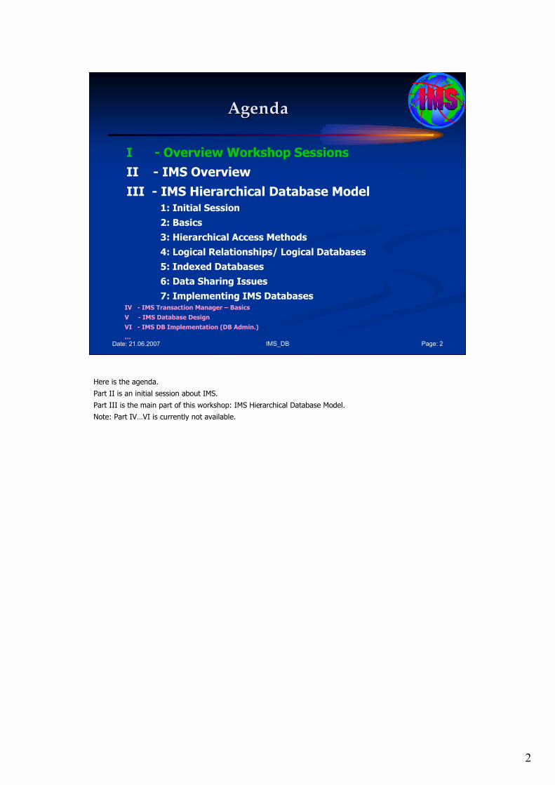
Here is the agenda.
Part II is an initial session about IMS.
Part III is the main part of this workshop: IMS Hierarchical Database Model.
Note: Part IV…VI is currently not available.

3
IMS_DB Page: 3Date: 21.06.2007
Let’s now start the sessions...
Workshop
The world depends on it
I hope this workshop is right for you! Enjoy the following sessions!

1
Date: 21.06.2007 IMS_02.ppt Page: 1
IBM Mainframe
IMS DB/DC
Presentation (Workshop)
Part II: IMS OverviewPart II: IMS Overview
June 2007 June 2007 –– 1st Version1st Version
presented bypresented by
Dipl. Dipl. IngIng. Werner Hoffmann. Werner Hoffmann
EMAIL: EMAIL: pwhoffmann @ tpwhoffmann @ t--online.deonline.de
A member of IEEE and ACM
Mainframe
Please see the notes pages for additional comments. Please see the notes pages for additional comments.
Welcome to the presentation (initial presentation/workshop) called “IMS DB/DC".
And welcome to the world of IMS, my still favorite world…
2
IMS_DB/DC Page: 2Date: 21.06.2007
Agenda
1. Term of IMS
2. Overview of the IMS product
3. An initial example
4. IMS DB and IMS TM
5. FAQ about TM/DB Basics
6. IMS Usage and Technology Trends
7. Summary
DB –Design Workshop:Point of Interest
Note:
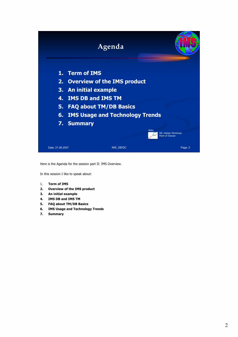
Here is the Agenda for the session part II: IMS Overview.
In this session I like to speak about:
1. Term of IMS
2. Overview of the IMS product
3. An initial example
4. IMS DB and IMS TM
5. FAQ about TM/DB Basics
6. IMS Usage and Technology Trends
7. Summary
3
IMS_DB/DC Page: 3Date: 21.06.2007
Agenda
1. Term of IMS
2. Overview of the IMS product
3. An initial example
4. IMS DB and IMS TM
5. FAQ about TM/DB Basics
6. IMS Usage and Technology Trends
7. Summary
Step 1: Term IMS

4
IMS_DB/DC Page: 4Date: 21.06.2007
Term of IMS…
IBM’s Information Management System(IMS) is a joint hierarchical database and information management system with extensive transaction processingcapability. Data Communication
Manager (DC) or IMS TM
Database Manager (DB)
Note: IMS DB/DC is not “IP Multimedia Subsystem (IMS)”!
IMS/ESA is an IBM program product that provides transaction management and database management functions for large commercial application systems. It was originally introduced in 1968. There are two major parts to IMS, a data communication manager (DC) and a Database Manager (DB).
IMS TM is a message-based transaction processor that is designed to use the OS/390 or MVS/ESA environment to your best advantage. IMS TM provides services to process messages received from the terminal network (input messages) and messages created by application programs (output messages). It also provides an underlying queuing mechanism for handling these messages.
IMS DB is a hierarchical database manager which provides an organization of business data with program and device independence. It has a built in data share capability.
It has been developed to provide an environment for applications that require very high levels of performance, throughput and availability. The development has been designed to make maximum use of the facilities of the operating system and hardware on which it runs, currently OS/390 or z/OS on S/390 or zSeries hardware.
Note: IBM Information Management System (IMS DC/DB) is one of the world’s premier software products. Period!
IMS is not in the news and is barely mentioned in today’s computer science classes, but it has been and, for the foreseeable future, will be continue to be, a major, crucial component of the world’s software infrastructure.
5
IMS_DB/DC Page: 5Date: 21.06.2007
Agenda
1. Term of IMS
2. Overview of the IMS product
3. An initial example
4. IMS DB and IMS TM
5. FAQ about TM/DB Basics
6. IMS Usage and Technology Trends
7. Summary
Step 2: Overview of the IMS product
6
IMS_DB/DC Page: 6Date: 21.06.2007
DB2
Overview of the IMS product
ACF/
VTAMSNA
Network
MVS
TCP/IPTCP/IP
Network
ITOC
MQ
Series
APPC/
MVS
IMS System
Services
Transaction
Management
Database
Manager
IMS
Message
Queues
DB2
Tables
IMS
Logs
MVS Console
IMS
Databases
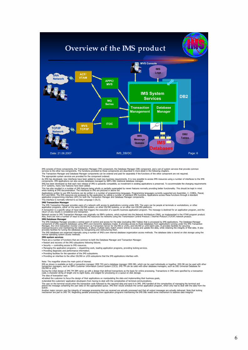
IMS consists of three components, the Transaction Manager (TM) component, the Database Manager (DB) component, and a set of system services that provide common services to the other two components. The functions provided by these components are described in more detail in the following chapters.
The Transaction Manager and Database Manager components can be ordered and paid for separately if the functions of the other component are not required.
The appropriate system services are provided for the component ordered.
As IMS has developed, new interfaces have been added to meet new business requirements. It is now possible to access IMS resources using a number of interfaces to the IMS components. IMS applications can also access databases managed by IBM’s DB2 relational database manager.
IMS has been developed so that each new release of IMS is upwardly compatible, so investment in existing applications is preserved. To accommodate the changing requirements of IT systems, many new features have been added.
This has also resulted in a number of IMS features being wholly or partially superseded by newer features normally providing better functionality. This should be kept in mind when looking at IMS documentation. The interfaces to IMS are pictured in above foil.
Applications written to use IMS functions can be written in a number of programming languages. Programming languages currently supported are Assembler, C, COBOL, Pascal, PL/I and REXX. The IMS resources are accessed by the application by calling a number of standard IMS functions. Applications access these functions through a standard application programming interface (API) for both the Transaction Manager and Database Manager components.
This interface is normally referred to as Data Language I (DL/I).
IMS Transaction Manager
The IMS Transaction Manager provides users of a network with access to applications running under IMS. The users can be people at terminals or workstations, or other application programs, either on the same OS/390 system, on other OS/390 systems, or on other non-OS/390 platforms.
A transaction is a specific setup of input data that triggers the execution of a specific business application program. The message is destined for an application program, and the return of any results is considered one transaction.
Network access to IMS Transaction Manager was originally via IBM’s systems, which evolved into the Network Architecture (SNA), as implemented in the VTAM program product. Also, there are now a number of ways to access IMS resources via networks using the Transmission Control Protocol / Internet Protocol (TCP/IP) network product.
IMS Database Manager
The IMS Database Manager provides a central point of control and access for the data (excluding DB2 Tables) that is processed by IMS applications. The Database Manager component of IMS supports databases using IMS’s own hierarchic database model. It provides access to these databases from applications running under the IMS Transaction Manager, the CICS transaction monitor (now known as Transaction Server for OS/390 or z/OS), and OS/390 or z/OS batch jobs. It provides facilities for securing (backup/recovery) and maintaining the databases. It allows multiple tasks (batch and/or online) to access and update the data, while retaining the integrity of that data. It also provides facilities for tuning the databases by reorganizing and restructuring them.
The IMS databases are organized internally using a number of IMS’s own internal database organization access methods. The database data is stored on disk storage using the normal operating system access methods.
IMS system services
There are a number of functions that are common to both the Database Manager and Transaction Manager:
• Restart and recovery of the IMS subsystems following failures.
• Security — controlling access to IMS resources.
• Managing the application programs — dispatching work, loading application programs, providing locking services.
• Providing diagnostic and performance information.
• Providing facilities for the operation of the IMS subsystems.
• Providing an interface to the other OS/390 or z/OS subsystems that the IMS applications interface with.
Note: The magnifier shows the main point of interest.
IMS as shown is available as both a transaction manager (IMS TM) and a database manager (IMS DB), which can be used individually or together. IMS DB can be used with other transaction managers, such as IBM’s Customer Information Control System (CICS). IMS TM can be used with other database managers, such as DB2 Universal Database for OS/390 or z/OS.
During the initial design of IMS TM IBM came up with a design that defined transactions as the basis for online processing. Transactions in IMS were specified by a transaction code, a character string of length one to eight bytes, and staged for processing on a queue on disk storage.
The idea of transaction was:
•Enabled the customer to focus the design of their applications on manipulating the data and implementing their business goals,
•Liberated the customers’ application developers from having to deal with the complexities of terminal communications.
The user on the terminal would enter the transaction code followed by the required data and send it to IMS. IMS handled all the complexities of managing the terminal and placed the message containing the user data on the appropriated queue. IMS then would schedule the correct application program, which only had to deal with the data from the queue.
Another major concern was the integrity of message processing that are received are actually processed and that all output messages are actually delivered. Note that locking mechanism are part to IMS TM. Regarding parallel processing even application programs maintaining the IMS DBs needs some mechanism to address data integrity!
7
IMS_DB/DC Page: 7Date: 21.06.2007
JAVA
Batch
Processing
MPPMPP
IMS control region
MPP
Application
Program
JAVAMPP
IFP
Application
Program
Fath Path DBs
LogsNetwork
IRLM
Region
IMS
System
DL/I
Separate
Address
Space
DBRC
Region
Full Function DBs RECONs
IMS Message Queues
IMS Libraries
Application RegionAddress Spaces
System AddressSpaces
ControlRegionAddressSpace
DependentRegionAddressSpaces
Legend:
MPPMPP
BMP
Application
Program
Message
Processing
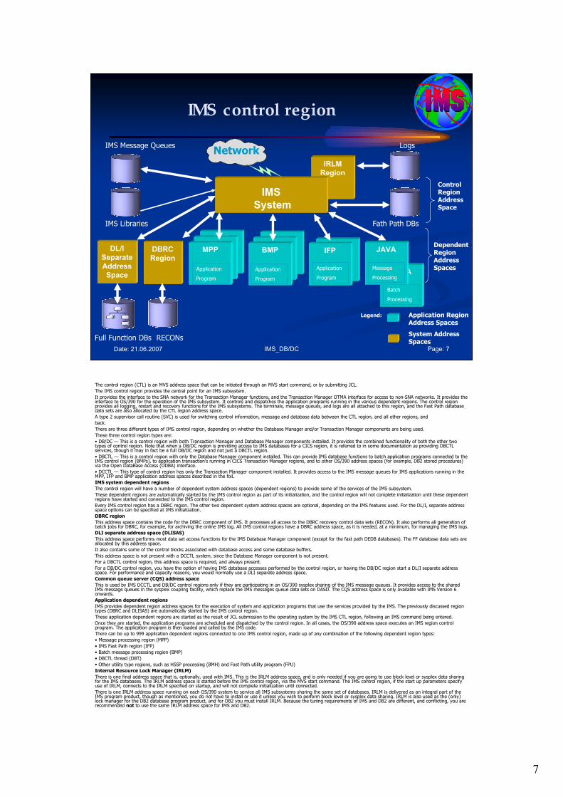
The control region (CTL) is an MVS address space that can be initiated through an MVS start command, or by submitting JCL.
The IMS control region provides the central point for an IMS subsystem.
It provides the interface to the SNA network for the Transaction Manager functions, and the Transaction Manager OTMA interface for access to non-SNA networks. It provides the interface to OS/390 for the operation of the IMS subsystem. It controls and dispatches the application programs running in the various dependent regions. The control region provides all logging, restart and recovery functions for the IMS subsystems. The terminals, message queues, and logs are all attached to this region, and the Fast Path database data sets are also allocated by the CTL region address space.
A type 2 supervisor call routine (SVC) is used for switching control information, message and database data between the CTL region, and all other regions, and
back.
There are three different types of IMS control region, depending on whether the Database Manager and/or Transaction Manager components are being used.
These three control region types are:
• DB/DC — This is a control region with both Transaction Manager and Database Manager components installed. It provides the combined functionality of both the other two types of control region. Note that when a DB/DC region is providing access to IMS databases for a CICS region, it is referred to in some documentation as providing DBCTL services, though it may in fact be a full DB/DC region and not just a DBCTL region.
• DBCTL — This is a control region with only the Database Manager component installed. This can provide IMS database functions to batch application programs connected to the IMS control region (BMPs), to application transaction’s running in CICS Transaction Manager regions, and to other OS/390 address spaces (for example, DB2 stored procedures) via the Open DataBase Access (ODBA) interface.
• DCCTL — This type of control region has only the Transaction Manager component installed. It provides access to the IMS message queues for IMS applications running in the MPP, IFP and BMP application address spaces described in the foil.
IMS system dependent regions
The control region will have a number of dependent system address spaces (dependent regions) to provide some of the services of the IMS subsystem.
These dependent regions are automatically started by the IMS control region as part of its initialization, and the control region will not complete initialization until these dependent regions have started and connected to the IMS control region.
Every IMS control region has a DBRC region. The other two dependent system address spaces are optional, depending on the IMS features used. For the DL/I, separate address space options can be specified at IMS initialization.
DBRC region
This address space contains the code for the DBRC component of IMS. It processes all access to the DBRC recovery control data sets (RECON). It also performs all generation of batch jobs for DBRC, for example, for archiving the online IMS log. All IMS control regions have a DBRC address space, as it is needed, at a minimum, for managing the IMS logs.
DLI separate address space (DLISAS)
This address space performs most data set access functions for the IMS Database Manager component (except for the fast path DEDB databases). The FF database data sets are allocated by this address space.
It also contains some of the control blocks associated with database access and some database buffers.
This address space is not present with a DCCTL system, since the Database Manager component is not present.
For a DBCTL control region, this address space is required, and always present.
For a DB/DC control region, you have the option of having IMS database accesses performed by the control region, or having the DB/DC region start a DL/I separate address space. For performance and capacity reasons, you would normally use a DLI separate address space.
Common queue server (CQS) address space
This is used by IMS DCCTL and DB/DC control regions only if they are participating in an OS/390 sysplex sharing of the IMS message queues. It provides access to the shared IMS message queues in the sysplex coupling facility, which replace the IMS messages queue data sets on DASD. The CQS address space is only available with IMS Version 6 onwards.
Application dependent regions
IMS provides dependent region address spaces for the execution of system and application programs that use the services provided by the IMS. The previously discussed region types (DBRC and DLISAS) are automatically started by the IMS control region.
These application dependent regions are started as the result of JCL submission to the operating system by the IMS CTL region, following an IMS command being entered.
Once they are started, the application programs are scheduled and dispatched by the control region. In all cases, the OS/390 address space executes an IMS region control program. The application program is then loaded and called by the IMS code.
There can be up to 999 application dependent regions connected to one IMS control region, made up of any combination of the following dependent region types:
• Message processing region (MPP)
• IMS Fast Path region (IFP)
• Batch message processing region (BMP)
• DBCTL thread (DBT)
• Other utility type regions, such as HSSP processing (BMH) and Fast Path utility program (FPU)
Internal Resource Lock Manager (IRLM)
There is one final address space that is, optionally, used with IMS. This is the IRLM address space, and is only needed if you are going to use block level or sysplex data sharing for the IMS databases. The IRLM address space is started before the IMS control region, via the MVS start command. The IMS control region, if the start up parameters specify use of IRLM, connects to the IRLM specified on startup, and will not complete initialization until connected.
There is one IRLM address space running on each OS/390 system to service all IMS subsystems sharing the same set of databases. IRLM is delivered as an integral part of the IMS program product, though as mentioned, you do not have to install or use it unless you wish to perform block level or sysplex data sharing. IRLM is also used as the (only) lock manager for the DB2 database program product, and for DB2 you must install IRLM. Because the tuning requirements of IMS and DB2 are different, and conflicting, you are recommended not to use the same IRLM address space for IMS and DB2.

8
IMS_DB/DC Page: 8Date: 21.06.2007
Agenda
1. Term of IMS
2. Overview of the IMS product
3. An initial example
4. IMS DB and IMS TM
5. FAQ about TM/DB Basics
6. IMS Usage and Technology Trends
7. Summary
Step 3: An initial example
9
IMS_DB/DC Page: 9Date: 21.06.2007
A Typical Manual System: Loan Application
CustomereXtendBank
Loan Officer
1. Fill in Loan
Application at Loan
Dept
2. Loan Officer enters
loan information (3270
emulator)
IMS
3. Requests
FAX Credit
Report
5. Makes a
decision on
Loan
Application
4. Makes decision as
to whether this Loan
application needs
approval.
6. Loan
Officer
reserves
Funds
7.Sends email to
Assess Business
Risk –
(Government
Watch List)
8. Notifies
customer
Business Analyst
(Rules change
frequently)
Developer
Loan Officer
Loan Officer Loan Officer Loan Officer Loan OfficerBank Manager
Application
Server
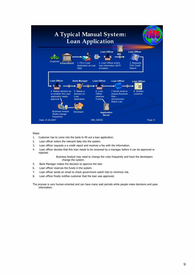
Steps:
1. Customer has to come into the bank to fill out a loan application.
2. Loan officer enters the relevant data into the system.
3. Loan officer requests a a credit report and receives a fax with the information.
4. Loan officer decides that this loan needs to be reviewed by a manager before it can be approved or rejected.
Business Analyst may need to change the rules frequently and have the developers change the system.
5. Bank Manager makes the decision to approve the loan
6. Loan officer reserves the funds in the system.
7. Loan officer sends an email to check government watch lists to minimize risk.
8. Loan officer finally notifies customer that the loan was approved.
The process is very human-oriented and can have many wait periods while people make decisions and pass information.
10
IMS_DB/DC Page: 10Date: 21.06.2007
Automated*) *) *) *)
computer assistedcomputer assisted
Loan Application Process
Start
Create Loan App
Credit Check
Pre-
approved?Loan Officer
Approval
ApproveReserve Funds
Assess Loan Risk
Too Risky?
Send Rejection Email
Send Confirmation Email
End
Service (Web)
Service (IMS)
Service (J2EE)
Service (Web)
Service (JavaMail)
Service (JavaMail)
12
YES
NO
NO
YES
YES
NO
LegendServices
Business Rules
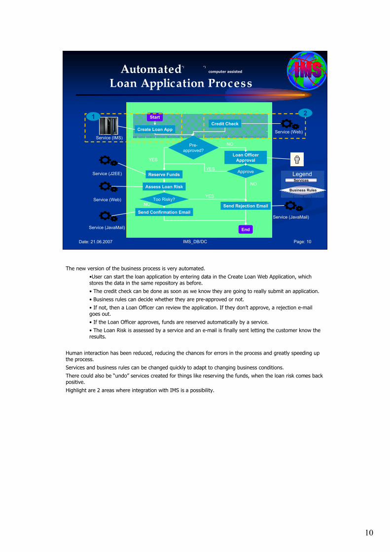
The new version of the business process is very automated.
•User can start the loan application by entering data in the Create Loan Web Application, which stores the data in the same repository as before.
• The credit check can be done as soon as we know they are going to really submit an application.
• Business rules can decide whether they are pre-approved or not.
• If not, then a Loan Officer can review the application. If they don’t approve, a rejection e-mail goes out.
• If the Loan Officer approves, funds are reserved automatically by a service.
• The Loan Risk is assessed by a service and an e-mail is finally sent letting the customer know the results.
Human interaction has been reduced, reducing the chances for errors in the process and greatly speeding up the process.
Services and business rules can be changed quickly to adapt to changing business conditions.
There could also be “undo” services created for things like reserving the funds, when the loan risk comes back positive.
Highlight are 2 areas where integration with IMS is a possibility.
11
IMS_DB/DC Page: 11Date: 21.06.2007
Scenario 1: Create an IMS Service
RetrieveCustInfo Import
binding=<“EIS”>
Create Loan App
Service (IMS)
1
CreateLoanApp
Impl = “Java”
IMS
Connector
for Java
IMS transaction is invoked and retrieves applicant information and returns it via the IMS resource adapter
ACF/
VTAMIMS DB/DC
IMS
DBs
Classical IMS DB/DC environment:
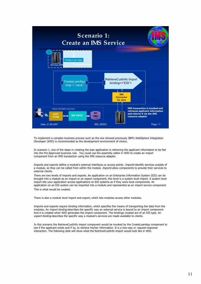
To implement a complex business process such as the one showed previously IBM’s WebSphere Integration Developer (WID) is recommended as the development environment of choice.
In scenario 1, one of the steps in creating the loan application is retrieving the applicant information to be fed into the Pre-Approved business rule. You could use the assembly editor in WID to create an import component from an IMS transaction using the IMS resource adapter.
Imports and exports define a module's external interfaces or access points. Imports identify services outside of a module, so they can be called from within the module. Exports allow components to provide their services to external clients.
There are two levels of imports and exports. An application on an Enterprise Information System (EIS) can be brought into a module as an import or an export component; this level is a system level import. A system level import lets your application access applications on EIS systems as if they were local components. An application on an EIS system can be imported into a module and represented as an import service component.
This is what would be created.
There is also a module level import and export, which lets modules access other modules.
Imports and exports require binding information, which specifies the means of transporting the data from the modules. An import binding describes the specific way an external service is bound to an import component. And it is created when WID generates the import component. The bindings created are of an EIS type. An export binding describes the specific way a module's services are made available to clients.
In this scenario the RetrieveCustInfo import component would be invoked by the CreateLoanApp component to see if the applicant exists and if so, to retrieve his/her information. It is a two-way or request-responseinteraction. The following slide will show what the RetrieveCustInfo import would look like in WID.
12
IMS_DB/DC Page: 12Date: 21.06.2007
Scenario 2: Create an IMS Web Service import
CreditCheck Import
binding = “WebService”
Credit Check
Service (Web)
2
LoanApp
Impl = “BPEL”
…
Application
IMS DB
IMS
Connect
IMS
Connector
for
Java
IMS DBDB2
Application ServerApplication
ApplicationIMS
TM
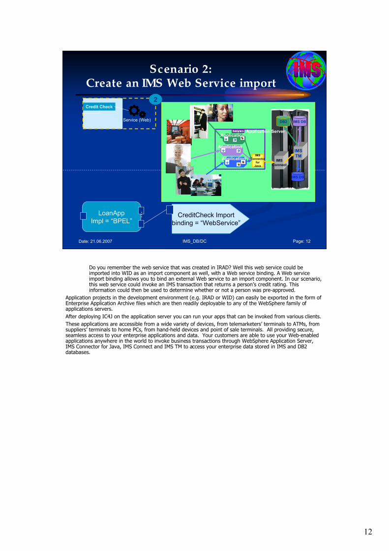
Do you remember the web service that was created in IRAD? Well this web service could be imported into WID as an import component as well, with a Web service binding. A Web service import binding allows you to bind an external Web service to an import component. In our scenario, this web service could invoke an IMS transaction that returns a person’s credit rating. This information could then be used to determine whether or not a person was pre-approved.
Application projects in the development environment (e.g. IRAD or WID) can easily be exported in the form of Enterprise Application Archive files which are then readily deployable to any of the WebSphere family of applications servers.
After deploying IC4J on the application server you can run your apps that can be invoked from various clients.
These applications are accessible from a wide variety of devices, from telemarketers’ terminals to ATMs, from suppliers’ terminals to home PCs, from hand-held devices and point of sale terminals. All providing secure,seamless access to your enterprise applications and data. Your customers are able to use your Web-enabled applications anywhere in the world to invoke business transactions through WebSphere Application Server, IMS Connector for Java, IMS Connect and IMS TM to access your enterprise data stored in IMS and DB2 databases.
13
IMS_DB/DC Page: 13Date: 21.06.2007
IMS TM & the World Wide Webthe World Wide Web
3270 Terminal
1,2
VTAM IMS MPP
3 4,5
8,9 7 6
NCP
Web Browser
1,2
WebServer
CGIProgram
3 4,5
8,9 7 6
TCP/IPTCP/IP
Program to ProgramCommunications

14
IMS_DB/DC Page: 14Date: 21.06.2007
Agenda
1. Term of IMS
2. Overview of the IMS product
3. An initial example
4. IMS DB and IMS TM
5. FAQ about TM/DB Basics
6. IMS Usage and Technology Trends
7. Summary
Step 4: IMS DB and IMS TM
15
IMS_DB/DC Page: 15Date: 21.06.2007
IMS is a Database Management System – IMS DB
ORDER
DETAIL/PART SHIPMENT
STOCK
Logical Database
Physical Databases
DETAIL
STOCK
PART
STOCK
ORDER
DETAIL SHIPMENT
PART
Physical DBORDER
Physical DB
IX-ADDR
Logical
Relationship
Secondary
Index
Source
Target
concatenated
segmentORDERSTOCKSTOCK
DEALER
STOCK
MODEL
ORDER
Hierarchical Database Model
Level
1
2
3
Parent
Child
Child
ChildTwins
DB
Segment
Type
Segments are
Implicit joined
with each
other
Siblings
Root Segment
Dependent Segment
Key
Key
Key
Key
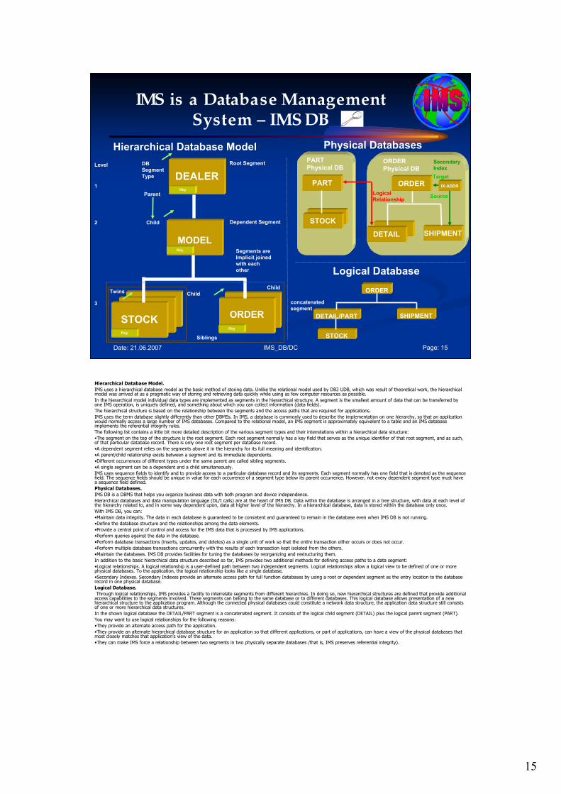
Hierarchical Database Model.
IMS uses a hierarchical database model as the basic method of storing data. Unlike the relational model used by DB2 UDB, which was result of theoretical work, the hierarchical model was arrived at as a pragmatic way of storing and retrieving data quickly while using as few computer resources as possible.
In the hierarchical model individual data types are implemented as segments in the hierarchical structure. A segment is the smallest amount of data that can be transferred by one IMS operation, is uniquely defined, and something about which you can collect information (data fields).
The hierarchical structure is based on the relationship between the segments and the access paths that are required for applications.
IMS uses the term database slightly differently than other DBMSs. In IMS, a database is commonly used to describe the implementation on one hierarchy, so that an application would normally access a large number of IMS databases. Compared to the relational model, an IMS segment is approximately equivalent to a table and an IMS database implements the referential integrity rules.
The following list contains a little bit more detailed description of the various segment types and their interrelations within a hierarchical data structure:
•The segment on the top of the structure is the root segment. Each root segment normally has a key field that serves as the unique identifier of that root segment, and as such, of that particular database record. There is only one root segment per database record.
•A dependent segment relies on the segments above it in the hierarchy for its full meaning and identification.
•A parent/child relationship exists between a segment and its immediate dependents.
•Different occurrences of different types under the same parent are called sibling segments.
•A single segment can be a dependent and a child simultaneously.
IMS uses sequence fields to identify and to provide access to a particular database record and its segments. Each segment normally has one field that is denoted as the sequence field. The sequence fields should be unique in value for each occurrence of a segment type below its parent occurrence. However, not every dependent segment type must have a sequence field defined.
Physical Databases.
IMS DB is a DBMS that helps you organize business data with both program and device independence.
Hierarchical databases and data manipulation language (DL/I calls) are at the heart of IMS DB. Data within the database is arranged in a tree structure, with data at each level of the hierarchy related to, and in some way dependent upon, data at higher level of the hierarchy. In a hierarchical database, data is stored within the database only once.
With IMS DB, you can:
•Maintain data integrity. The data in each database is guaranteed to be consistent and guaranteed to remain in the database even when IMS DB is not running.
•Define the database structure and the relationships among the data elements.
•Provide a central point of control and access for the IMS data that is processed by IMS applications.
•Perform queries against the data in the database.
•Perform database transactions (inserts, updates, and deletes) as a single unit of work so that the entire transaction either occurs or does not occur.
•Perform multiple database transactions concurrently with the results of each transaction kept isolated from the others.
•Maintain the databases. IMS DB provides facilities for tuning the databases by reorganizing and restructuring them.
In addition to the basic hierarchical data structure described so far, IMS provides two additional methods for defining access paths to a data segment:
•Logical relationships. A logical relationship is a user-defined path between two independent segments. Logical relationships allow a logical view to be defined of one or more physical databases. To the application, the logical relationship looks like a single database.
•Secondary Indexes. Secondary Indexes provide an alternate access path for full function databases by using a root or dependent segment as the entry location to the database record in one physical database.
Logical Database.
Through logical relationships, IMS provides a facility to interrelate segments from different hierarchies. In doing so, new hierarchical structures are defined that provide additional access capabilities to the segments involved. These segments can belong to the same database or to different databases. This logical database allows presentation of a new hierarchical structure to the application program. Although the connected physical databases could constitute a network data structure, the application data structure still consists of one or more hierarchical data structures.
In the shown logical database the DETAIL/PART segment is a concatenated segment. It consists of the logical child segment (DETAIL) plus the logical parent segment (PART).
You may want to use logical relationships for the following reasons:
•They provide an alternate access path for the application.
•They provide an alternate hierarchical database structure for an application so that different applications, or part of applications, can have a view of the physical databases that most closely matches that application’s view of the data.
•They can make IMS force a relationship between two segments in two physically separate databases /that is, IMS preserves referential integrity).
16
IMS_DB/DC Page: 16Date: 21.06.2007
IMS is a Database Management System
A
B C
D E
IMS DB is organized hierarchically
� To optimize storage and retrieval
� To ensure integrity and recovery
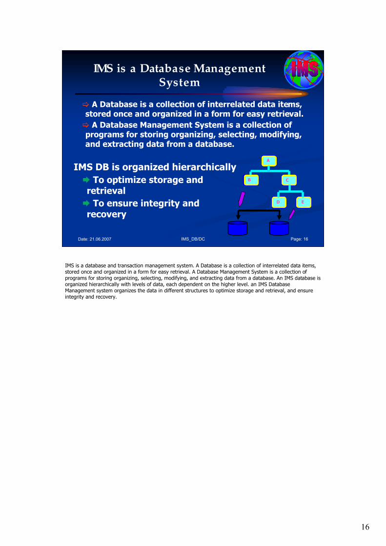
� A Database is a collection of interrelated data items, stored once and organized in a form for easy retrieval.
� A Database Management System is a collection of programs for storing organizing, selecting, modifying, and extracting data from a database.
IMS is a database and transaction management system. A Database is a collection of interrelated data items, stored once and organized in a form for easy retrieval. A Database Management System is a collection of programs for storing organizing, selecting, modifying, and extracting data from a database. An IMS database is organized hierarchically with levels of data, each dependent on the higher level. an IMS Database Management system organizes the data in different structures to optimize storage and retrieval, and ensure integrity and recovery.
17
IMS_DB/DC Page: 17Date: 21.06.2007
Program Structure Program Structure –– Data FlowData Flow(Traditional)(Traditional)
Application Program – (Batch)
PROGRAM ENTRY
DEFINE PSB (PCB AREAS)
GET INPUT RECORDS FROM INPUT FILE
CALLS TO DL/I DB FUNCTIONS
RETRIEVEINSERTREPLACEDELETE
CHECK STATUS CODES
PUT OUTPUT RECORDS
TERMINATION
IOAREAPrefix
Segment
visible in
Application program
Segments Segmentsto/from to/from
databasesdatabases
E
N
T
R
y
E
X
I
T
DLI modules
Call from
from DLI
PCB-Mask
IO AREA
PSB
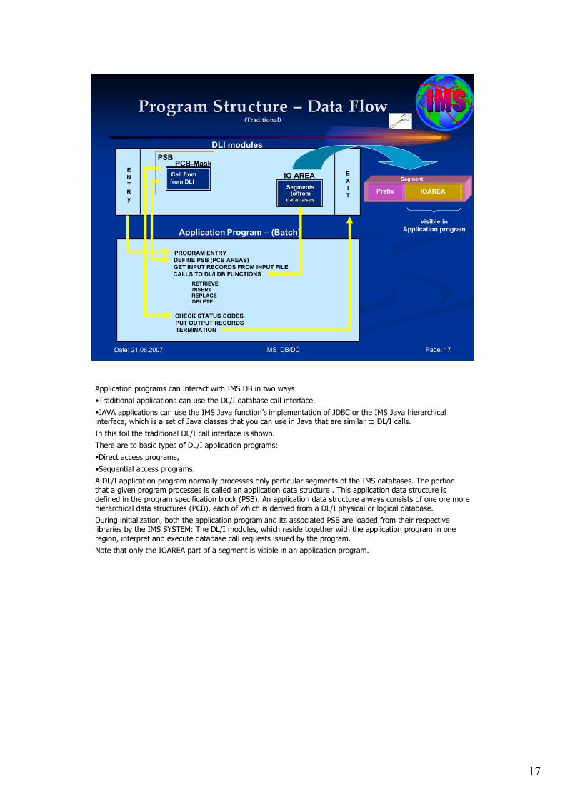
Application programs can interact with IMS DB in two ways:
•Traditional applications can use the DL/I database call interface.
•JAVA applications can use the IMS Java function’s implementation of JDBC or the IMS Java hierarchical interface, which is a set of Java classes that you can use in Java that are similar to DL/I calls.
In this foil the traditional DL/I call interface is shown.
There are to basic types of DL/I application programs:
•Direct access programs,
•Sequential access programs.
A DL/I application program normally processes only particular segments of the IMS databases. The portion that a given program processes is called an application data structure . This application data structure is defined in the program specification block (PSB). An application data structure always consists of one ore more hierarchical data structures (PCB), each of which is derived from a DL/I physical or logical database.
During initialization, both the application program and its associated PSB are loaded from their respective libraries by the IMS SYSTEM: The DL/I modules, which reside together with the application program in one region, interpret and execute database call requests issued by the program.
Note that only the IOAREA part of a segment is visible in an application program.
18
IMS_DB/DC Page: 18Date: 21.06.2007
Data Characteristics
Application Oriented
Limited Integration
Constantly Updated
Current Values Only
Supports Daily Operations
Operational Data
Subject Oriented
Integrated
Non-volatile
Values Over Time
Supports Decision Making
Informational Data
Operational and Informational Data Fundamentally Different
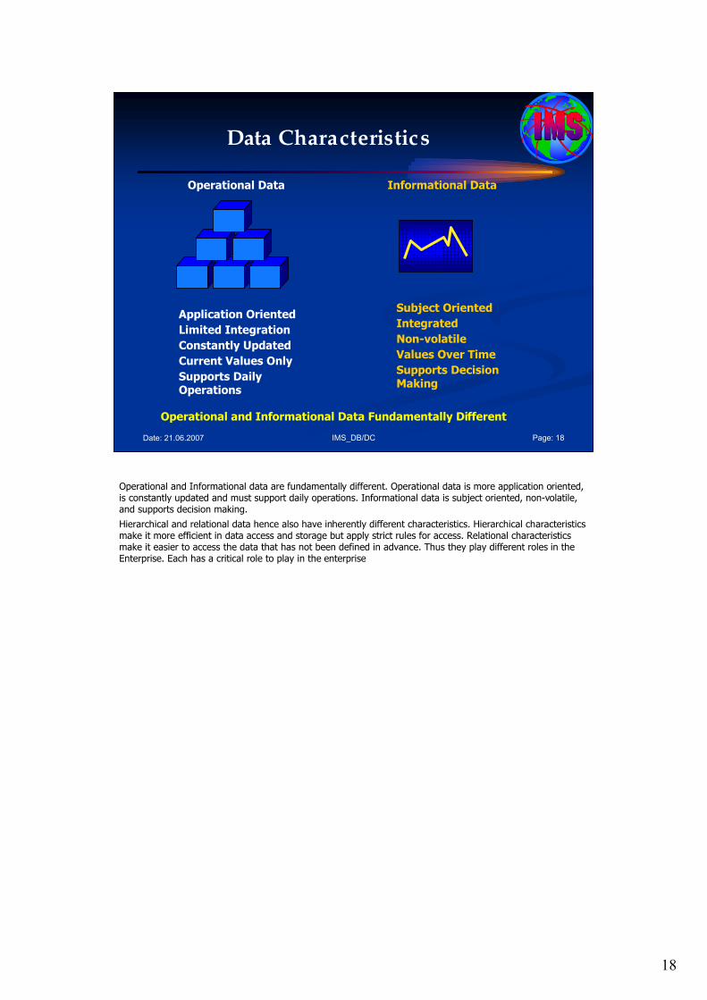
Operational and Informational data are fundamentally different. Operational data is more application oriented, is constantly updated and must support daily operations. Informational data is subject oriented, non-volatile, and supports decision making.
Hierarchical and relational data hence also have inherently different characteristics. Hierarchical characteristics make it more efficient in data access and storage but apply strict rules for access. Relational characteristics make it easier to access the data that has not been defined in advance. Thus they play different roles in the Enterprise. Each has a critical role to play in the enterprise
19
IMS_DB/DC Page: 19Date: 21.06.2007
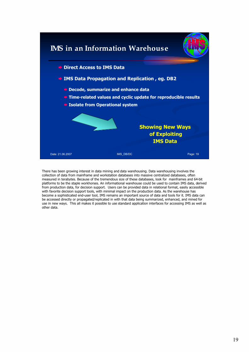
IMS in an Information Warehouse
� Direct Access to IMS Data
� IMS Data Propagation and Replication , eg. DB2
� Decode, summarize and enhance data
� Time-related values and cyclic update for reproducible results
� Isolate from Operational system
Showing New Ways
of Exploiting
IMS Data
There has been growing interest in data mining and data warehousing. Data warehousing involves the collection of data from mainframe and workstation databases into massive centralized databases, often measured in terabytes. Because of the tremendous size of these databases, look for mainframes and 64-bit platforms to be the staple workhorses. An informational warehouse could be used to contain IMS data, derived from production data, for decision support. Users can be provided data in relational format, easily accessible with favorite decision support tools, with minimal impact on the production data. As the warehouse has become a sophisticated end-user tool, IMS remains an important source of data and tools for it. IMS data can be accessed directly or propagated/replicated in with that data being summarized, enhanced, and mined for use in new ways. This all makes it possible to use standard application interfaces for accessing IMS as well as other data.
20
IMS_DB/DC Page: 20Date: 21.06.2007
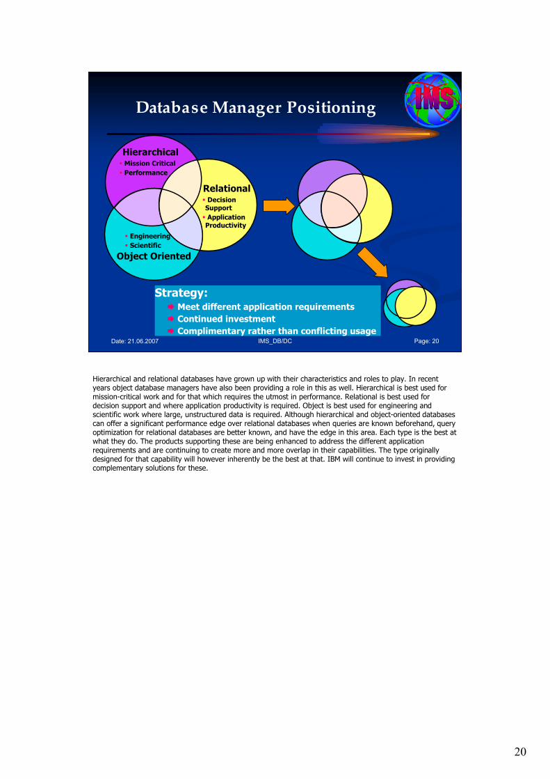
Database Manager Positioning
Strategy:� Meet different application requirements
� Continued investment
� Complimentary rather than conflicting usage
Hierarchical� Mission Critical
� Performance
Relational� Decision Support
� Application Productivity
� Engineering
� Scientific
Object Oriented
Hierarchical and relational databases have grown up with their characteristics and roles to play. In recent years object database managers have also been providing a role in this as well. Hierarchical is best used for mission-critical work and for that which requires the utmost in performance. Relational is best used for decision support and where application productivity is required. Object is best used for engineering and scientific work where large, unstructured data is required. Although hierarchical and object-oriented databases can offer a significant performance edge over relational databases when queries are known beforehand, query optimization for relational databases are better known, and have the edge in this area. Each type is the best at what they do. The products supporting these are being enhanced to address the different application requirements and are continuing to create more and more overlap in their capabilities. The type originally designed for that capability will however inherently be the best at that. IBM will continue to invest in providing complementary solutions for these.
21
IMS_DB/DC Page: 21Date: 21.06.2007
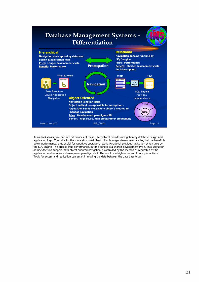
Database Management Systems -Differentiation
HierarchicalNavigation done apriori by database
design & application logic
Price: Longer development cycle
Benefit: Performance
RelationalNavigation done at run time by
'SQL' engine
Price: Performance
Benefit: Shorter development cycle
decision support
Propagation
SQL
Engine
Application
SQL Engine
Provides
Independence
HowWhat
Method
1
Data
Method
2
Method
3
Navigation
Object OrientedNavigation is not an issue
Object method is responsible for navigation -
Application sends message to object's method to
manage navigation
Price: Development paradigm shift
Benefit: High reuse, high programmer productivity
Data Structure
Drives Application
Navigation
Application
What & How?
As we look closer, you can see differences of these. Hierarchical provides navigation by database design and application logic. The price for the more structured hierarchical is longer development cycles, but the benefit is better performance, thus useful for repetitive operational work. Relational provides navigation at run time by the SQL engine. The price is thus performance, but the benefit is a shorter development cycle, thus useful for ad-hoc decision support. With object oriented navigation is controlled by the method as requested by the application and requires a development paradigm shift. The result is a high reuse and future productivity. Tools for access and replication can assist in moving the data between the data base types.
22
IMS_DB/DC Page: 22Date: 21.06.2007
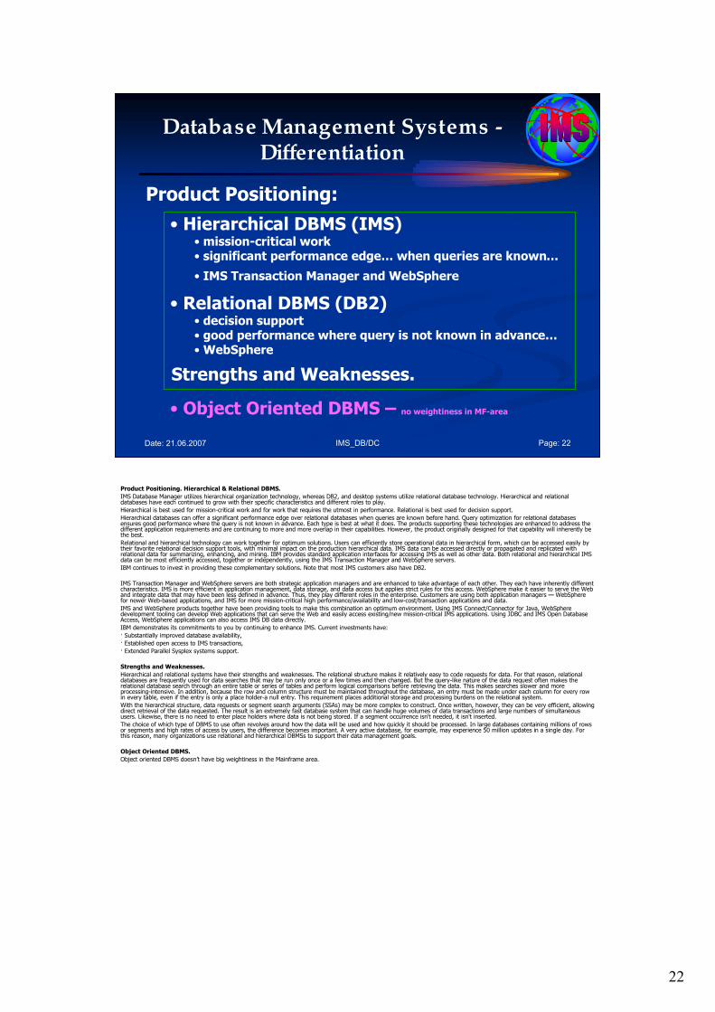
Database Management Systems -Differentiation
Product Positioning:
• Hierarchical DBMS (IMS)• mission-critical work• significant performance edge… when queries are known…
• IMS Transaction Manager and WebSphere
• Relational DBMS (DB2)• decision support• good performance where query is not known in advance…• WebSphere
Strengths and Weaknesses.
• Object Oriented DBMS – no weightiness in MF-area
Product Positioning. Hierarchical & Relational DBMS.
IMS Database Manager utilizes hierarchical organization technology, whereas DB2, and desktop systems utilize relational database technology. Hierarchical and relational databases have each continued to grow with their specific characteristics and different roles to play.
Hierarchical is best used for mission-critical work and for work that requires the utmost in performance. Relational is best used for decision support.
Hierarchical databases can offer a significant performance edge over relational databases when queries are known before hand. Query optimization for relational databases ensures good performance where the query is not known in advance. Each type is best at what it does. The products supporting these technologies are enhanced to address the different application requirements and are continuing to more and more overlap in their capabilities. However, the product originally designed for that capability will inherently be the best.
Relational and hierarchical technology can work together for optimum solutions. Users can efficiently store operational data in hierarchical form, which can be accessed easily by their favorite relational decision support tools, with minimal impact on the production hierarchical data. IMS data can be accessed directly or propagated and replicated with relational data for summarizing, enhancing, and mining. IBM provides standard application interfaces for accessing IMS as well as other data. Both relational and hierarchical IMS data can be most efficiently accessed, together or independently, using the IMS Transaction Manager and WebSphere servers.
IBM continues to invest in providing these complementary solutions. Note that most IMS customers also have DB2.
IMS Transaction Manager and WebSphere servers are both strategic application managers and are enhanced to take advantage of each other. They each have inherently different characteristics. IMS is more efficient in application management, data storage, and data access but applies strict rules for this access. WebSphere make it easier to serve the Web and integrate data that may have been less defined in advance. Thus, they play different roles in the enterprise. Customers are using both application managers — WebSpherefor newer Web-based applications, and IMS for more mission-critical high performance/availability and low-cost/transaction applications and data.
IMS and WebSphere products together have been providing tools to make this combination an optimum environment. Using IMS Connect/Connector for Java, WebSpheredevelopment tooling can develop Web applications that can serve the Web and easily access existing/new mission-critical IMS applications. Using JDBC and IMS Open Database Access, WebSphere applications can also access IMS DB data directly.
IBM demonstrates its commitments to you by continuing to enhance IMS. Current investments have:
� Substantially improved database availability,
� Established open access to IMS transactions,
� Extended Parallel Sysplex systems support.
Strengths and Weaknesses.
Hierarchical and relational systems have their strengths and weaknesses. The relational structure makes it relatively easy to code requests for data. For that reason, relational databases are frequently used for data searches that may be run only once or a few times and then changed. But the query-like nature of the data request often makes the relational database search through an entire table or series of tables and perform logical comparisons before retrieving the data. This makes searches slower and more processing-intensive. In addition, because the row and column structure must be maintained throughout the database, an entry must be made under each column for every row in every table, even if the entry is only a place holder-a null entry. This requirement places additional storage and processing burdens on the relational system.
With the hierarchical structure, data requests or segment search arguments (SSAs) may be more complex to construct. Once written, however, they can be very efficient, allowing direct retrieval of the data requested. The result is an extremely fast database system that can handle huge volumes of data transactions and large numbers of simultaneous users. Likewise, there is no need to enter place holders where data is not being stored. If a segment occurrence isn't needed, it isn't inserted.
The choice of which type of DBMS to use often revolves around how the data will be used and how quickly it should be processed. In large databases containing millions of rows or segments and high rates of access by users, the difference becomes important. A very active database, for example, may experience 50 million updates in a single day. For this reason, many organizations use relational and hierarchical DBMSs to support their data management goals.
Object Oriented DBMS.
Object oriented DBMS doesn’t have big weightiness in the Mainframe area.
23
IMS_DB/DC Page: 23Date: 21.06.2007
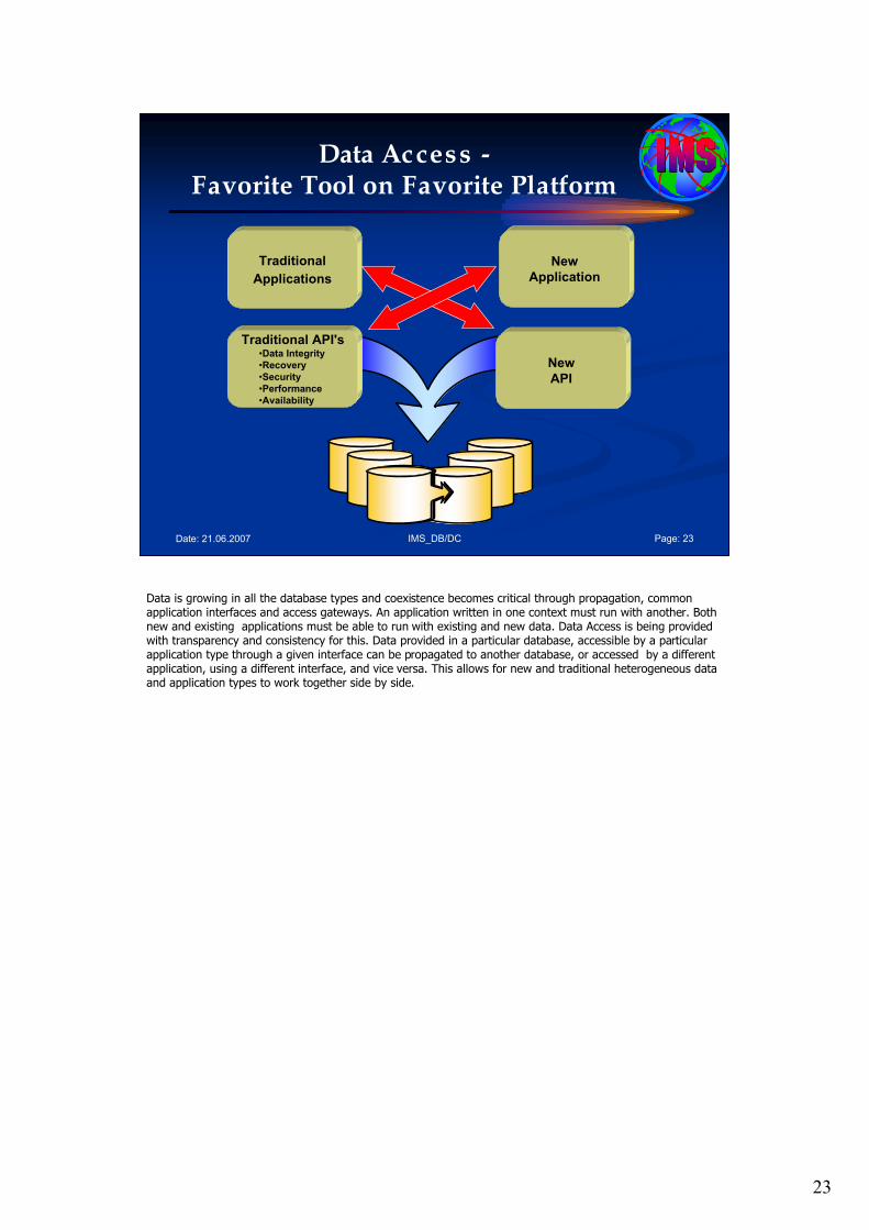
Data Access -Favorite Tool on Favorite Platform
Traditional
Applications
Traditional API's•Data Integrity
•Recovery
•Security
•Performance
•Availability
New
Application
New
API
Data is growing in all the database types and coexistence becomes critical through propagation, common application interfaces and access gateways. An application written in one context must run with another. Both new and existing applications must be able to run with existing and new data. Data Access is being provided with transparency and consistency for this. Data provided in a particular database, accessible by a particular application type through a given interface can be propagated to another database, or accessed by a different application, using a different interface, and vice versa. This allows for new and traditional heterogeneous data and application types to work together side by side.
24
IMS_DB/DC Page: 24Date: 21.06.2007
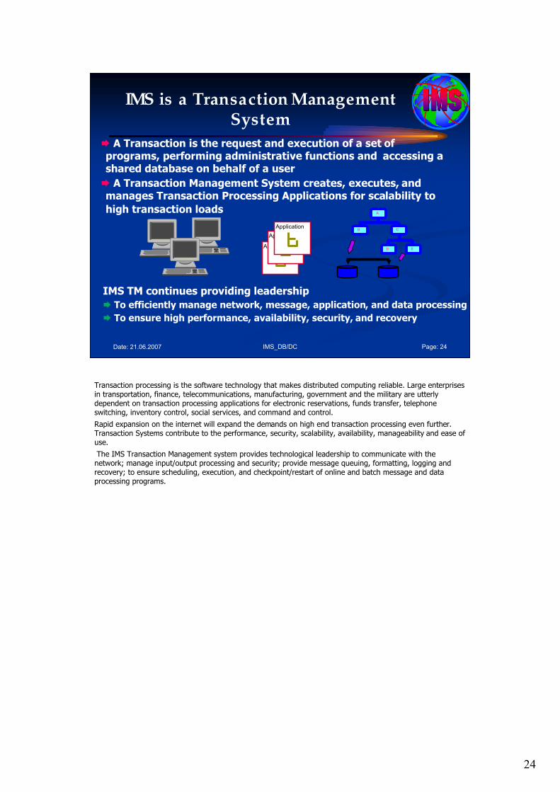
IMS is a Transaction Management System
A
B C
D EApplication
Application
Application
IMS TM continues providing leadership
� To efficiently manage network, message, application, and data processing
� To ensure high performance, availability, security, and recovery
� A Transaction is the request and execution of a set of programs, performing administrative functions and accessing a shared database on behalf of a user
� A Transaction Management System creates, executes, and manages Transaction Processing Applications for scalability to
high transaction loads
Transaction processing is the software technology that makes distributed computing reliable. Large enterprises in transportation, finance, telecommunications, manufacturing, government and the military are utterly dependent on transaction processing applications for electronic reservations, funds transfer, telephone switching, inventory control, social services, and command and control.
Rapid expansion on the internet will expand the demands on high end transaction processing even further. Transaction Systems contribute to the performance, security, scalability, availability, manageability and ease of use.
The IMS Transaction Management system provides technological leadership to communicate with the network; manage input/output processing and security; provide message queuing, formatting, logging and recovery; to ensure scheduling, execution, and checkpoint/restart of online and batch message and data processing programs.
25
IMS_DB/DC Page: 25Date: 21.06.2007
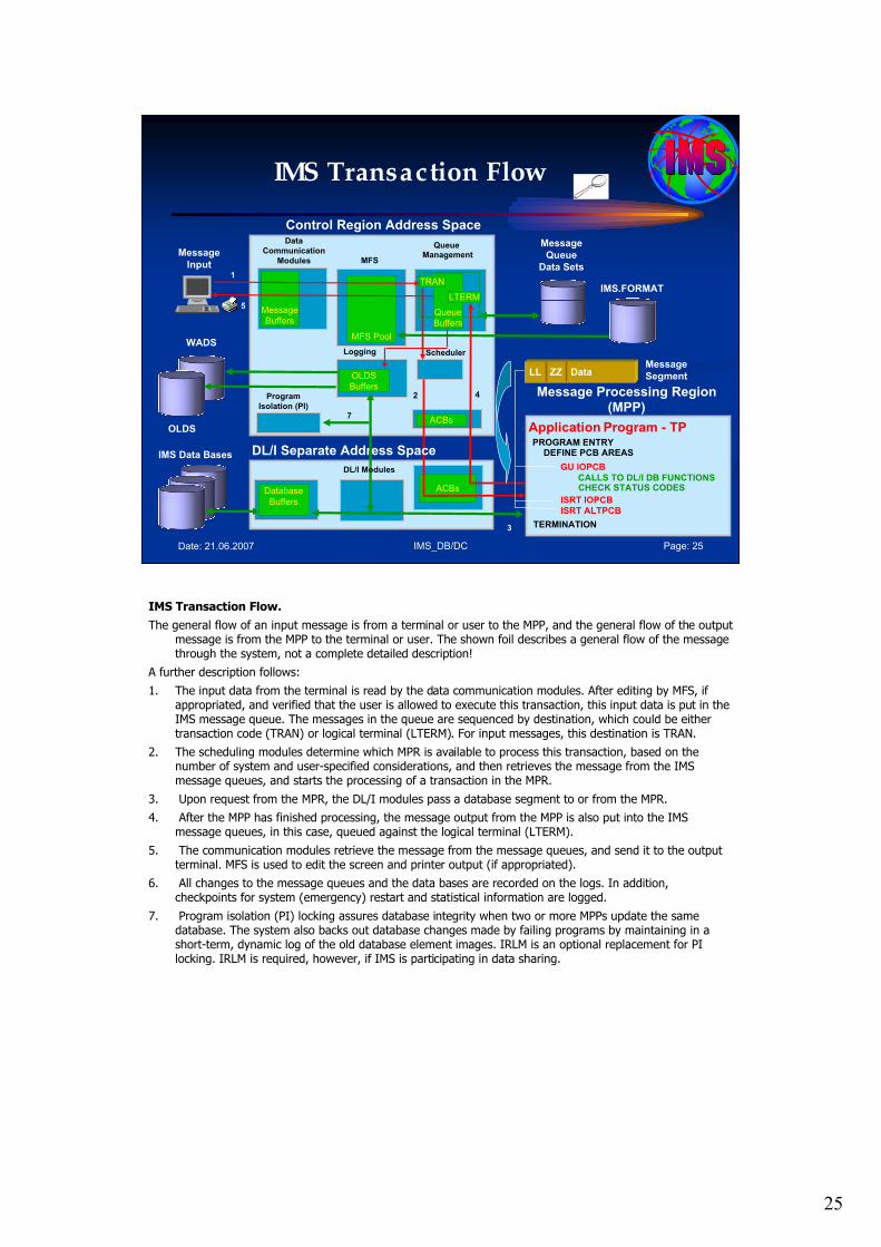
IMS Transaction Flow
Control Region Address Space
MessageBuffers
Data
Communication
Modules
Queue Management
Application Program - TPPROGRAM ENTRYDEFINE PCB AREAS
CALLS TO DL/I DB FUNCTIONSCHECK STATUS CODES
TERMINATION
MFS Pool
MFSMessage
Input
Message
Queue
Data Sets
IMS.FORMAT
OLDSBuffers
LoggingWADS
OLDS
Program
Isolation (PI)
Scheduler
ACBs
ACBsDatabase
Buffers
GU IOPCB
ISRT IOPCBISRT ALTPCB
DL/I Separate Address Space
Message Processing Region(MPP)
IMS Data Bases
DL/I Modules
LL ZZ Data Message
Segment
1
2
3
4
QueueBuffers
TRAN
LTERM5
7
IMS Transaction Flow.
The general flow of an input message is from a terminal or user to the MPP, and the general flow of the output message is from the MPP to the terminal or user. The shown foil describes a general flow of the message through the system, not a complete detailed description!
A further description follows:
1. The input data from the terminal is read by the data communication modules. After editing by MFS, if appropriated, and verified that the user is allowed to execute this transaction, this input data is put in the IMS message queue. The messages in the queue are sequenced by destination, which could be either transaction code (TRAN) or logical terminal (LTERM). For input messages, this destination is TRAN.
2. The scheduling modules determine which MPR is available to process this transaction, based on the number of system and user-specified considerations, and then retrieves the message from the IMS message queues, and starts the processing of a transaction in the MPR.
3. Upon request from the MPR, the DL/I modules pass a database segment to or from the MPR.
4. After the MPP has finished processing, the message output from the MPP is also put into the IMS message queues, in this case, queued against the logical terminal (LTERM).
5. The communication modules retrieve the message from the message queues, and send it to the output terminal. MFS is used to edit the screen and printer output (if appropriated).
6. All changes to the message queues and the data bases are recorded on the logs. In addition, checkpoints for system (emergency) restart and statistical information are logged.
7. Program isolation (PI) locking assures database integrity when two or more MPPs update the same database. The system also backs out database changes made by failing programs by maintaining in a short-term, dynamic log of the old database element images. IRLM is an optional replacement for PI locking. IRLM is required, however, if IMS is participating in data sharing.
26
IMS_DB/DC Page: 26Date: 21.06.2007
Agenda
1. Term of IMS
2. Overview of the IMS product
3. An initial example
4. IMS DB and IMS TM
5. FAQ about TM/DB Basics
6. IMS Usage and Technology Trends
7. Summary
Step 5: FAQ about IMS TM and IMS DB Basics.
27
IMS_DB/DC Page: 27Date: 21.06.2007
Why not just Data Systems ?
Database
Management
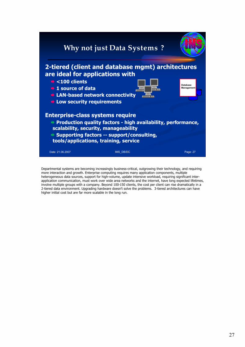
2-tiered (client and database mgmt) architectures are ideal for applications with
� <100 clients
� 1 source of data
� LAN-based network connectivity
� Low security requirements
Enterprise-class systems require
� Production quality factors - high availability, performance, scalability, security, manageability
� Supporting factors -- support/consulting, tools/applications, training, service
Departmental systems are becoming increasingly business-critical, outgrowing their technology, and requiring more interaction and growth. Enterprise computing requires many application components, multiple heterogeneous data sources, support for high-volume, update intensive workload, requiring significant inter-application communication, must work over wide area networks and the internet, have long expected lifetimes, involve multiple groups with a company. Beyond 100-150 clients, the cost per client can rise dramatically in a 2-tiered data environment. Upgrading hardware doesn't solve the problems. 3-tiered architectures can have higher initial cost but are far more scalable in the long run.
28
IMS_DB/DC Page: 28Date: 21.06.2007
Why Transaction Management ?
Transaction Management
Database
Management
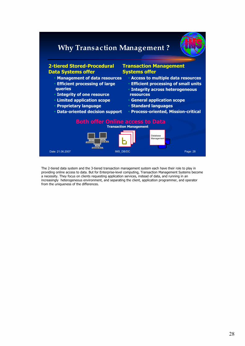
2-tiered Stored-Procedural Data Systems offer
� Management of data resources
� Efficient processing of large queries
� Integrity of one resource
� Limited application scope
� Proprietary language
� Data-oriented decision support
Transaction Management Systems offer
� Access to multiple data resources
� Efficient processing of small units
� Integrity across heterogeneous resources
� General application scope
� Standard languages
� Process-oriented, Mission-critical
Both offer Online access to Data
The 2-tiered data system and the 3-tiered transaction management system each have their role to play in providing online access to data. But for Enterprise-level computing, Transaction Management Systems become a necessity. They focus on clients requesting application services, instead of data, and running in an increasingly heterogeneous environment, and separating the client, application programmer, and operator from the uniqueness of the differences.
29
IMS_DB/DC Page: 29Date: 21.06.2007
Why Transaction Management ?
Transaction Management
Both offer Online access to Data
Database
ManagementEnterprise Application ServersApplication Platform Suites
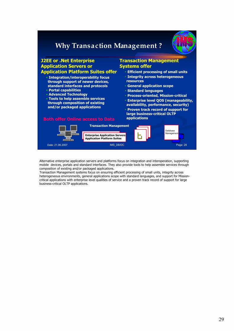
J2EE or .Net Enterprise Application Servers or Application Platform Suites offer
• Integration/interoperability focus through support of newer devices, standard interfaces and protocols
• Portal capabilities • Advanced Technology • Tools to help assemble services through composition of existing and/or packaged applications
Transaction Management Systems offer
� Efficient processing of small units
� Integrity across heterogeneous resources
� General application scope
� Standard languages
� Process-oriented, Mission-critical
� Enterprise level QOS (manageability, availability, performance, security)
� Proven track record of support for large business-critical OLTP applications
Alternative enterprise application servers and platforms focus on integration and interoperation, supporting mobile devices, portals and standard interfaces. They also provide tools to help assemble services through composition of existing and/or packaged applications.Transaction Management systems focus on ensuring efficient processing of small units, integrity across heterogeneous environments, general applications scope with standard languages, and support for Mission-critical applications with enterprise level qualities of service and a proven track record of support for large business-critical OLTP applications.
30
IMS_DB/DC Page: 30Date: 21.06.2007
Why IMS Transaction Management ?
IMS Transaction Management
Database
Management
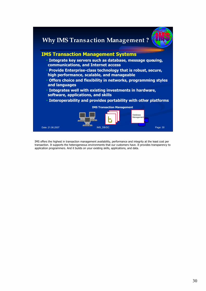
IMS Transaction Management Systems� Integrate key servers such as database, message queuing, communications, and Internet access
� Provide Enterprise-class technology that is robust, secure, high performance, scalable, and manageable
� Offers choice and flexibility in networks, programming styles and languages
� Integrates well with existing investments in hardware, software, applications, and skills
� Interoperability and provides portability with other platforms
IMS offers the highest in transaction management availability, performance and integrity at the least cost per transaction. It supports the heterogeneous environments that our customers have. It provides transparency to application programmers. And it builds on your existing skills, applications, and data.
31
IMS_DB/DC Page: 31Date: 21.06.2007
Agenda
1. Term of IMS
2. Overview of the IMS product
3. An initial example
4. IMS DB and IMS TM
5. FAQ about TM/DB Basics
6. IMS Usage and Technology Trends
7. Summary
Step 6: IMS Usage and Technology Trends.

32
IMS_DB/DC Page: 32Date: 21.06.2007
Overall Message:IMS is an evolving, thriving species –that is CORE to your business
Born to beBorn to be…… a Winner!a Winner!
Overall Message: IMS is an evolving, thriving species –that is CORE to your business
All great things seem to start in a box. Many successful motorcycle companies started out in small garages or shacks – an idea, a place to tinker. IMS started in a box: the System 360/65 computer (pictured is the operator’s console).
Then the hard work and innovation takes off – winning races (first racing bike and first rocket to the moon (Apollo program)), and defining ‘cool’ - (the cruisers (a style of motorcycle) and access 24/7 to your cold hard cash (the ATM))...
And a good thing keeps on going – with modern superbike designs that push the limit speed, and hardware (the z9) that blows away anything in its path.
But, at the heart of both are powerful engines. IMS is a powerful engine that continues to adapt and grow –helping you and your company win…
33
IMS_DB/DC Page: 33Date: 21.06.2007
The World Depends on IMS
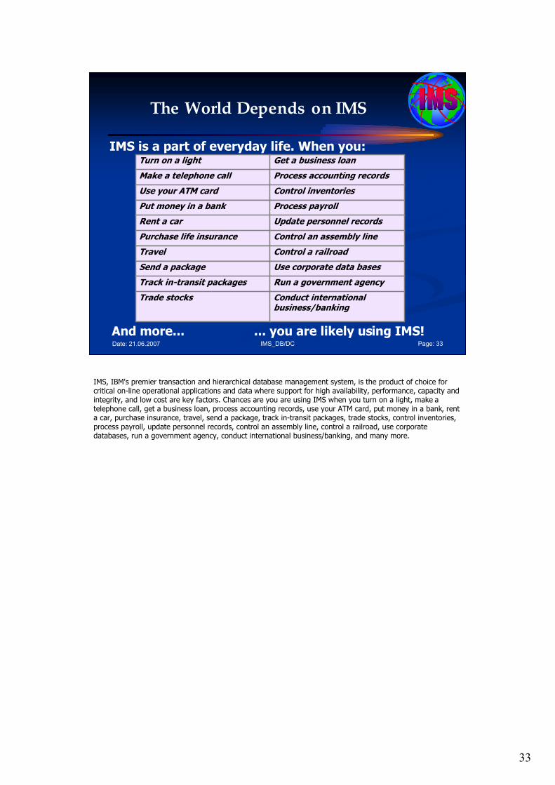
IMS is a part of everyday life. When you: Turn on a light Get a business loan
Make a telephone call Process accounting records
Use your ATM card Control inventories
Put money in a bank Process payroll
Rent a car Update personnel records
Purchase life insurance Control an assembly line
Travel Control a railroad
Send a package Use corporate data bases
Track in-transit packages Run a government agency
Trade stocks Conduct international business/banking
And more... ... you are likely using IMS!
IMS, IBM's premier transaction and hierarchical database management system, is the product of choice for critical on-line operational applications and data where support for high availability, performance, capacity and integrity, and low cost are key factors. Chances are you are using IMS when you turn on a light, make a telephone call, get a business loan, process accounting records, use your ATM card, put money in a bank, rent a car, purchase insurance, travel, send a package, track in-transit packages, trade stocks, control inventories, process payroll, update personnel records, control an assembly line, control a railroad, use corporate databases, run a government agency, conduct international business/banking, and many more.
34
IMS_DB/DC Page: 34Date: 21.06.2007
The World Depends on IMS
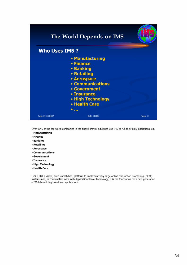
• Manufacturing• Finance• Banking• Retailing• Aerospace• Communications• Government• Insurance• High Technology• Health Care• …
Who Uses IMS ?
Over 90% of the top world companies in the above shown industries use IMS to run their daily operations, eg.
• Manufacturing
• Finance
• Banking
• Retailing
• Aerospace
• Communications
• Government
• Insurance
• High Technology
• Health Care
IMS is still a viable, even unmatched, platform to implement very large online transaction processing (OLTP) systems and, in combination with Web Application Server technology, it is the foundation for a new generation of Web-based, high-workload applications.
35
IMS_DB/DC Page: 35Date: 21.06.2007
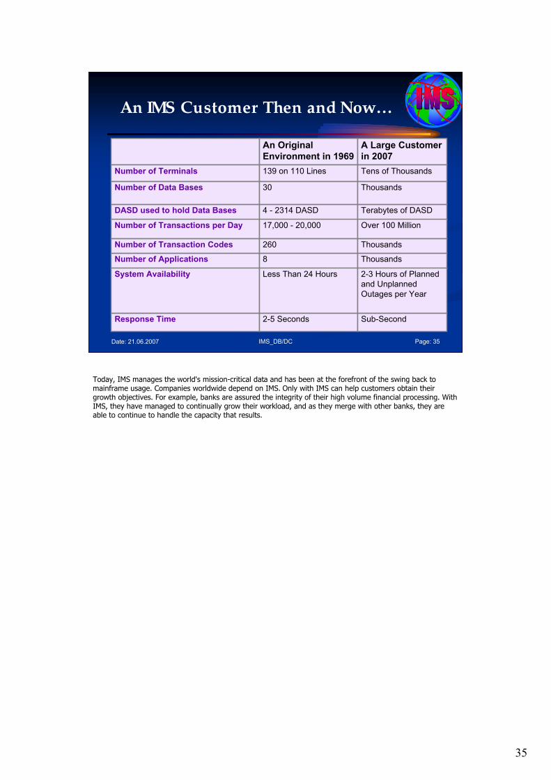
An IMS Customer Then and Now…
Number of Terminals
Number of Data Bases
DASD used to hold Data Bases
Number of Transactions per Day
Number of Transaction Codes
Number of Applications
System Availability
Response Time
An Original
Environment in 1969
139 on 110 Lines
30
4 - 2314 DASD
17,000 - 20,000
260
8
Less Than 24 Hours
2-5 Seconds
A Large Customer
in 2007
Tens of Thousands
Thousands
Terabytes of DASD
Over 100 Million
Thousands
Thousands
2-3 Hours of Planned
and Unplanned
Outages per Year
Sub-Second
Today, IMS manages the world's mission-critical data and has been at the forefront of the swing back tomainframe usage. Companies worldwide depend on IMS. Only with IMS can help customers obtain their growth objectives. For example, banks are assured the integrity of their high volume financial processing. With IMS, they have managed to continually grow their workload, and as they merge with other banks, they are able to continue to handle the capacity that results.
36
IMS_DB/DC Page: 36Date: 21.06.2007
IMS Runs the World...
Most Corporate Data is Managed by IMS� Over 95% of top Fortune 1000 Companies use IMS� IMS Manages over 15 Billion GBs of Production Data
� $2.5 Trillion/day transferred through IMS by one customer
Over 50 Billion Transactions a Day run through IMS� IMS Serves Close to 200 Million Users a Day� Over 100 Million IMS Trans/Day Handled by One Customer on a single system� 120M IMS Trans/day, 7M per hour handled by another customer� 6000 Trans/sec across TCP/IP to single IMS with a single Connect instance� Over 21,000 Trans/sec (near 2 Billion/day) with IMS Data/Queued sharing on a
single processor
Gartner Group: "A large and loyal IMS installed base. Rock-solid reputation of a transactional workhorse for very large workloads. Successfully proven in large, Web-based applications. IMS is still a viable, even unmatched, platform to implement very large OLTP systems, and, in combination with Web Application Server technology, it can be a foundation for a new generation of Web-based, high-workload applications."
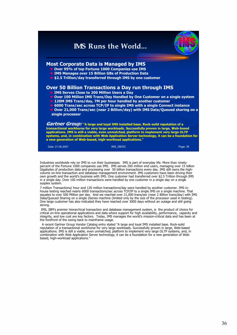
Industries worldwide rely on IMS to run their businesses. IMS is part of everyday life. More than ninety-percent of the Fortune 1000 companies use IMS. IMS serves 200 million end users, managing over 15 billion Gigabytes of production data and processing over 50 billion transactions every day. IMS still owns the high-volume on-line transaction and database management environment. IMS customers have been driving their own growth and the world's business with IMS. One customer had transferred over $2.5 Trillion through IMS in a single day. Over 100 million transactions were handled by one customer in a single day on a single sysplex system.
7 million Transactions/ hour and 120 million transactions/day were handled by another customer. IMS in-house testing reached nearly 6000 transactions/sec across TCP/IP to a single IMS on a single machine. That equates to over 500 Million per day. And we reached over 21,000 trans/sec (near 2 Billion trans/day) with IMS Data/Queued Sharing on a single zSeries machine (limited only by the size of the processor used in testing). One large customer has also indicated they have reached over 3000 days without an outage and still going strong.
IMS, IBM's premier hierarchical transaction and database management system, is the product of choice for critical on-line operational applications and data where support for high availability, performance, capacity and integrity, and low cost are key factors. Today, IMS manages the world's mission-critical data and has been at the forefront of the swing back to mainframe usage.
A recent Gartner Group Vendor Catalog entry stated "A large and loyal IMS installed base. Rock-solid reputation of a transactional workhorse for very large workloads. Successfully proven in large, Web-based applications. IMS is still a viable, even unmatched, platform to implement very large OLTP systems, and, in combination with Web Application Server technology, it can be a foundation for a new generation of Web-based, high-workload applications."
37
IMS_DB/DC Page: 37Date: 21.06.2007
IMS Today
� Command processing
� Memory Management
� Operations Interface
� Global resource management
� Inter-systems communications
� Network Management
� Message Management
� Data communications
� Security
� Organize
� Store and Retrieve
� Data Integrity
� Recoverability
Network Access
CICS
DB2 Stored
Procedures
Single Point
of Control
Control
Center
Operations Management
Mainframe Workstation
zOS
Transaction
Management
Systems
Services
Database
Management
IMS
Websphere
DB2 IMS DB
Java
Integrated
Connect
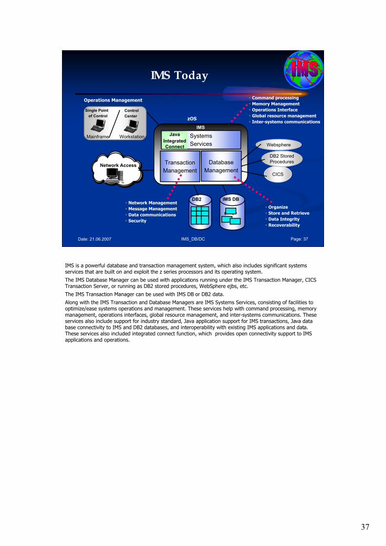
IMS is a powerful database and transaction management system, which also includes significant systems services that are built on and exploit the z series processors and its operating system.
The IMS Database Manager can be used with applications running under the IMS Transaction Manager, CICS Transaction Server, or running as DB2 stored procedures, WebSphere ejbs, etc.
The IMS Transaction Manager can be used with IMS DB or DB2 data.
Along with the IMS Transaction and Database Managers are IMS Systems Services, consisting of facilities to optimize/ease systems operations and management. These services help with command processing, memory management, operations interfaces, global resource management, and inter-systems communications. These services also include support for industry standard, Java application support for IMS transactions, Java data base connectivity to IMS and DB2 databases, and interoperability with existing IMS applications and data. These services also included integrated connect function, which provides open connectivity support to IMS applications and operations.
38
IMS_DB/DC Page: 38Date: 21.06.2007
IMS: 39+ years and stillleading the industry!!!
Data Base Concurrent Update
From Multiple User/System
Multiple Systems Coupling (MSC)
Batch
DBMS
Exploit MP
Architecture
Two Phase
Commit
Deadlock Detection
> 2500 Transactions
Per Second
Local Hot Standby DBMS (XRF)
1968
2007+
Concurrent Image Copy
Parallel Systems N-Way Data Sharing
2-way Data Sharing
Remote Site Recovery
APPC/IMS
Internet Access
Shared Message
Queues
...Extended Terminal Option (ETO)
Web Services
> 1000 Transactions
Per Second
> 22000 Transactions
Per Second
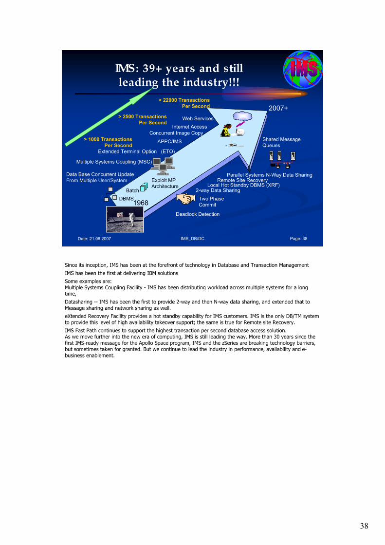
Since its inception, IMS has been at the forefront of technology in Database and Transaction Management
IMS has been the first at delivering IBM solutions
Some examples are: Multiple Systems Coupling Facility - IMS has been distributing workload across multiple systems for a long time,
Datasharing -- IMS has been the first to provide 2-way and then N-way data sharing, and extended that to Message sharing and network sharing as well.
eXtended Recovery Facility provides a hot standby capability for IMS customers. IMS is the only DB/TM system to provide this level of high availability takeover support; the same is true for Remote site Recovery.
IMS Fast Path continues to support the highest transaction per second database access solution.As we move further into the new era of computing, IMS is still leading the way. More than 30 years since the first IMS-ready message for the Apollo Space program, IMS and the zSeries are breaking technology barriers, but sometimes taken for granted. But we continue to lead the industry in performance, availability and e-business enablement.
39
IMS_DB/DC Page: 39Date: 21.06.2007
IMS in a Parallel Sysplex
Easier access and management of enterprise applications and data
Allocation
of workstations
Dynamic
Workload
Balancing
Data
Sharing� IMS DB
� DB2
VTAM
IMS TM
VTAM
IMS TM
VTAM
IMS TM
IMS
TM
IMS DB
DB2
Lock
Manager
IMS
TM
IMS DB
DB2
Lock
Manager
IMS
TM
IMS DB
DB2
Lock
Manager
MSG
Queue
Locks
Directories
Caches
Coupling Facility
IMS DB2
Database Database
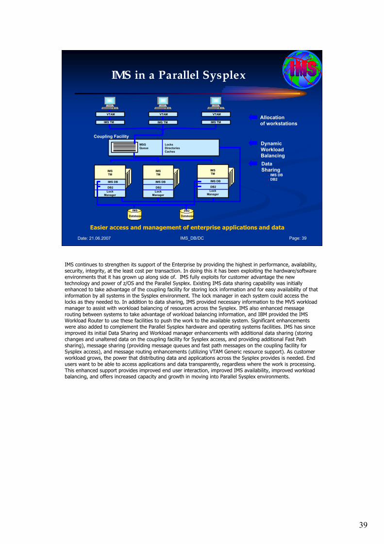
IMS continues to strengthen its support of the Enterprise by providing the highest in performance, availability, security, integrity, at the least cost per transaction. In doing this it has been exploiting the hardware/software environments that it has grown up along side of. IMS fully exploits for customer advantage the new technology and power of z/OS and the Parallel Sysplex. Existing IMS data sharing capability was initially enhanced to take advantage of the coupling facility for storing lock information and for easy availability of that information by all systems in the Sysplex environment. The lock manager in each system could access the locks as they needed to. In addition to data sharing, IMS provided necessary information to the MVS workload manager to assist with workload balancing of resources across the Sysplex. IMS also enhanced message routing between systems to take advantage of workload balancing information, and IBM provided the IMS Workload Router to use these facilities to push the work to the available system. Significant enhancements were also added to complement the Parallel Sysplex hardware and operating systems facilities. IMS has since improved its initial Data Sharing and Workload manager enhancements with additional data sharing (storing changes and unaltered data on the coupling facility for Sysplex access, and providing additional Fast Path sharing), message sharing (providing message queues and fast path messages on the coupling facility for Sysplex access), and message routing enhancements (utilizing VTAM Generic resource support). As customer workload grows, the power that distributing data and applications across the Sysplex provides is needed. End users want to be able to access applications and data transparently, regardless where the work is processing. This enhanced support provides improved end user interaction, improved IMS availability, improved workload balancing, and offers increased capacity and growth in moving into Parallel Sysplex environments.

40
IMS_DB/DC Page: 40Date: 21.06.2007
IMS and zSeries Breaking Barriers in Scalability
Benchmarked over 22,000 IMS Transactions/Second with Database Update on a SINGLE SYSTEM
Approximately 2 billion transactions/day
IMS V9 continues to leverage zSeries leadership capabilities offering a broad range of scalability and continually increasing performance/ capacity
Practically limitless volumes of data
Increased l/O bandwidth
Faster shared queues and shared data
Significantly more transaction throughput
IMS is designed, built and tuned to exploit the IBM Mainframe, leveraging the scalability, stability and technology advances on this platform. The zArchitecture will continue to provide growth and protect your enterprise computing investment well into the future.
What other platform provides the ability to demonstrate over 22,000 IMS transactions per second with database update on a single system? The latest versions of IMS and IBM System z9 hardware provide even higher levels of throughput and performance – managing even larger amounts of data and transactions.
41
IMS_DB/DC Page: 41Date: 21.06.2007
Ensuring Availability with IMS
END USER COMPONENT SYSTEM COMPONENT
Parallel Sysplex Support
IMS XRF, FDBR
Duplex DSs - MADS, Logs,
RECONs...
Multiple Address Space Design
Auto Opns
Programmed Operator Interface
Self Adjusting Governors
Application Task Isolation
/O Error Toleration
eXtended Restart Facility
Remote Site Recovery
Application vs System Isolation
Controlled Resource Allocation
System/Application
Checkpoint/Restart
Measure
Document
Resolve
Daylight Savings Support
ETO, OLC, VTAM GR
MADS, Dynamic OLDS/WADS
PDB, Online Reorg
XRF
Parallel Sysplex Exploitation
XRF
Online Data Reorg / Backup
Block Level Data Sharing
BMPs
Dynamic Allocation
Fault
Tolerance
Fault
Avoidance
Environmental
Independence
Failure-resistant
Applications
Availability
Management
Non-disruptive
Change
Non-disruptive
Maintenance
Continuous
Applications
High
Availability
** UNPLANNED
**
** OUTAGE
**
Continuous
Operations
** PLANNED **
** OUTAGE **
Continuous
Availability
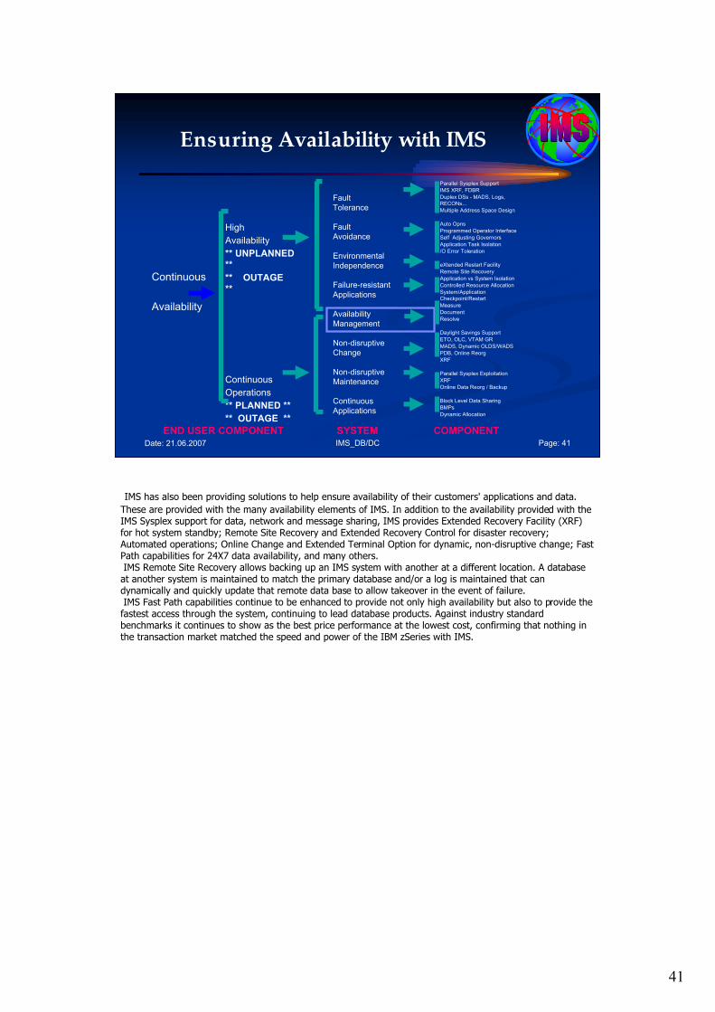
IMS has also been providing solutions to help ensure availability of their customers' applications and data.
These are provided with the many availability elements of IMS. In addition to the availability provided with the IMS Sysplex support for data, network and message sharing, IMS provides Extended Recovery Facility (XRF) for hot system standby; Remote Site Recovery and Extended Recovery Control for disaster recovery; Automated operations; Online Change and Extended Terminal Option for dynamic, non-disruptive change; Fast Path capabilities for 24X7 data availability, and many others.IMS Remote Site Recovery allows backing up an IMS system with another at a different location. A database at another system is maintained to match the primary database and/or a log is maintained that can dynamically and quickly update that remote data base to allow takeover in the event of failure. IMS Fast Path capabilities continue to be enhanced to provide not only high availability but also to provide the fastest access through the system, continuing to lead database products. Against industry standard benchmarks it continues to show as the best price performance at the lowest cost, confirming that nothing in the transaction market matched the speed and power of the IBM zSeries with IMS.

42
IMS_DB/DC Page: 42Date: 21.06.2007
Total Cost of Ownership
Performance/Scalability
Availability
Tools & Utilities
Systems Management
Education and Skills
The total cost of ownership is much more than software and hardware costs. We continue to work on a wide range of items where you have concerns.
The ability to scale as far as you need and using the processing capability efficiently continues to be a key concern.
The cost of an outage can be tens of thousands of dollars per minute, so extending our traditional strength is crucial.
Many customers pay more for tools and utilities than for the base products. We are helping to provide better value for the money.
Systems management is key. Enhancements are being designed/delivered to ease IMS systems management and move toward Autonomic Computing.
Finding people with S/390 and z/OS education and skills has become more and more difficult. We not only are trying to ease use and management of the system to bring down the skill level requirements, but to also provide certification programs, training and working with universities to continue building up our skill base.
43
IMS_DB/DC Page: 43Date: 21.06.2007
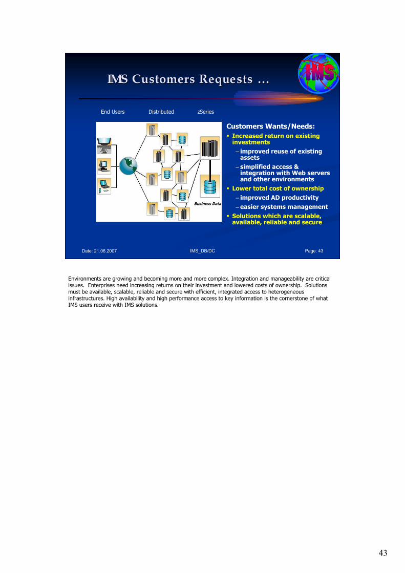
IMS Customers Requests IMS Customers Requests ……
Business Data
End Users Distributed zSeries
Customers Wants/Needs:
� Increased return on existing investments
– improved reuse of existing assets
– simplified access & integration with Web servers and other environments
� Lower total cost of ownership
– improved AD productivity
– easier systems management
� Solutions which are scalable, available, reliable and secure
Environments are growing and becoming more and more complex. Integration and manageability are critical issues. Enterprises need increasing returns on their investment and lowered costs of ownership. Solutions must be available, scalable, reliable and secure with efficient, integrated access to heterogeneous infrastructures. High availability and high performance access to key information is the cornerstone of what IMS users receive with IMS solutions.
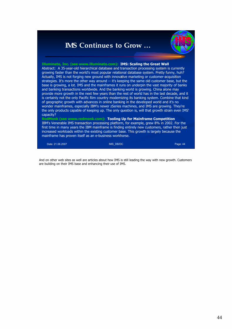
44
IMS_DB/DC Page: 44Date: 21.06.2007
IMS Continues to Grow …
Illuminata, Inc. (see www.illuminata.com): IMS: Scaling the Great Wall Abstract: A 35-year-old hierarchical database and transaction processing system is currently growing faster than the world's most popular relational database system. Pretty funny, huh? Actually, IMS is not forging new ground with innovative marketing or customer-acquisition strategies. It's more the other way around -- it's keeping the same old customer base, but the base is growing, a lot. IMS and the mainframes it runs on underpin the vast majority of banks and banking transactions worldwide. And the banking world is growing. China alone may provide more growth in the next few years than the rest of world has in the last decade, and it is certainly not the only Pacific Rim country modernizing its banking system. Combine that kind of geographic growth with advances in online banking in the developed world and it's no wonder mainframes, especially IBM's newer zSeries machines, and IMS are growing. They're the only products capable of keeping up. The only question is, will that growth strain even IMS' capacity?RedMonk (see www.redmonk.com): Tooling Up for Mainframe Competition IBM's Venerable IMS transaction processing platform, for example, grew 8% in 2002. For the first time in many years the IBM mainframe is finding entirely new customers, rather then just increased workloads within the existing customer base. This growth is largely because the mainframe has proven itself as an e-business workhorse.
And on other web sites as well are articles about how IMS is still leading the way with new growth. Customers are building on their IMS base and enhancing their use of IMS.
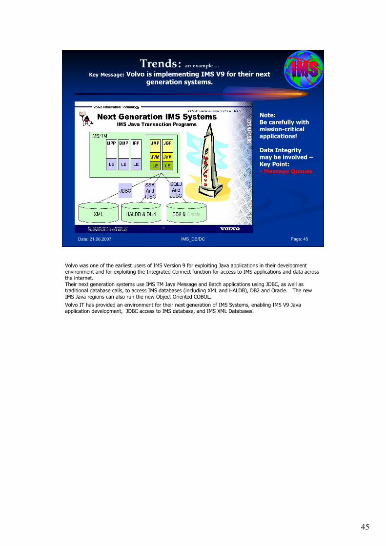
45
IMS_DB/DC Page: 45Date: 21.06.2007
Trends: an example …
Key Message: Volvo is implementing IMS V9 for their next generation systems.
Note:Be carefully withmission-criticalapplications!
Data Integritymay be involved –Key Point:• Message Queues
Volvo was one of the earliest users of IMS Version 9 for exploiting Java applications in their development environment and for exploiting the Integrated Connect function for access to IMS applications and data across the internet. Their next generation systems use IMS TM Java Message and Batch applications using JDBC, as well as traditional database calls, to access IMS databases (including XML and HALDB), DB2 and Oracle. The new IMS Java regions can also run the new Object Oriented COBOL.
Volvo IT has provided an environment for their next generation of IMS Systems, enabling IMS V9 Java application development, JDBC access to IMS database, and IMS XML Databases.
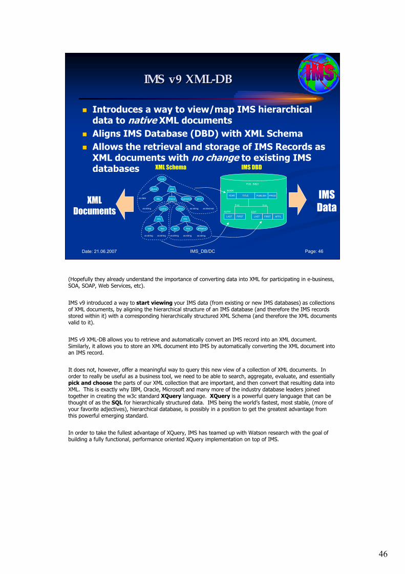
46
IMS_DB/DC Page: 46Date: 21.06.2007
IMS v9 XMLIMS v9 XML--DBDB
� Introduces a way to view/map IMS hierarchical data to native XML documents
� Aligns IMS Database (DBD) with XML Schema
� Allows the retrieval and storage of IMS Records as XML documents with no change to existing IMS databases
book
@year
title
seq
pricepublisherchoice
author
last first
seq
editor
last first
seq
affiliation
xs:date
xs:string
xs:string xs:string xs:string xs:string xs:string
xs:string xs:decimal
TITLE PUBLISH
FIRSTLAST FIRST
0:oo0:oo
AUTH EDIT
BOOK
YEAR PRICE
LAST AFFIL
PCB: BIB21
XML Schema IMS DBD
XML
Documents
IMS
Data
(Hopefully they already understand the importance of converting data into XML for participating in e-business, SOA, SOAP, Web Services, etc).
IMS v9 introduced a way to start viewing your IMS data (from existing or new IMS databases) as collections of XML documents, by aligning the hierarchical structure of an IMS database (and therefore the IMS records stored within it) with a corresponding hierarchically structured XML Schema (and therefore the XML documents valid to it).
IMS v9 XML-DB allows you to retrieve and automatically convert an IMS record into an XML document. Similarly, it allows you to store an XML document into IMS by automatically converting the XML document into an IMS record.
It does not, however, offer a meaningful way to query this new view of a collection of XML documents. In order to really be useful as a business tool, we need to be able to search, aggregate, evaluate, and essentially pick and choose the parts of our XML collection that are important, and then convert that resulting data into XML. This is exactly why IBM, Oracle, Microsoft and many more of the industry database leaders joined together in creating the w3c standard XQuery language. XQuery is a powerful query language that can be thought of as the SQL for hierarchically structured data. IMS being the world’s fastest, most stable, (more of your favorite adjectives), hierarchical database, is possibly in a position to get the greatest advantage from this powerful emerging standard.
In order to take the fullest advantage of XQuery, IMS has teamed up with Watson research with the goal of building a fully functional, performance oriented XQuery implementation on top of IMS.
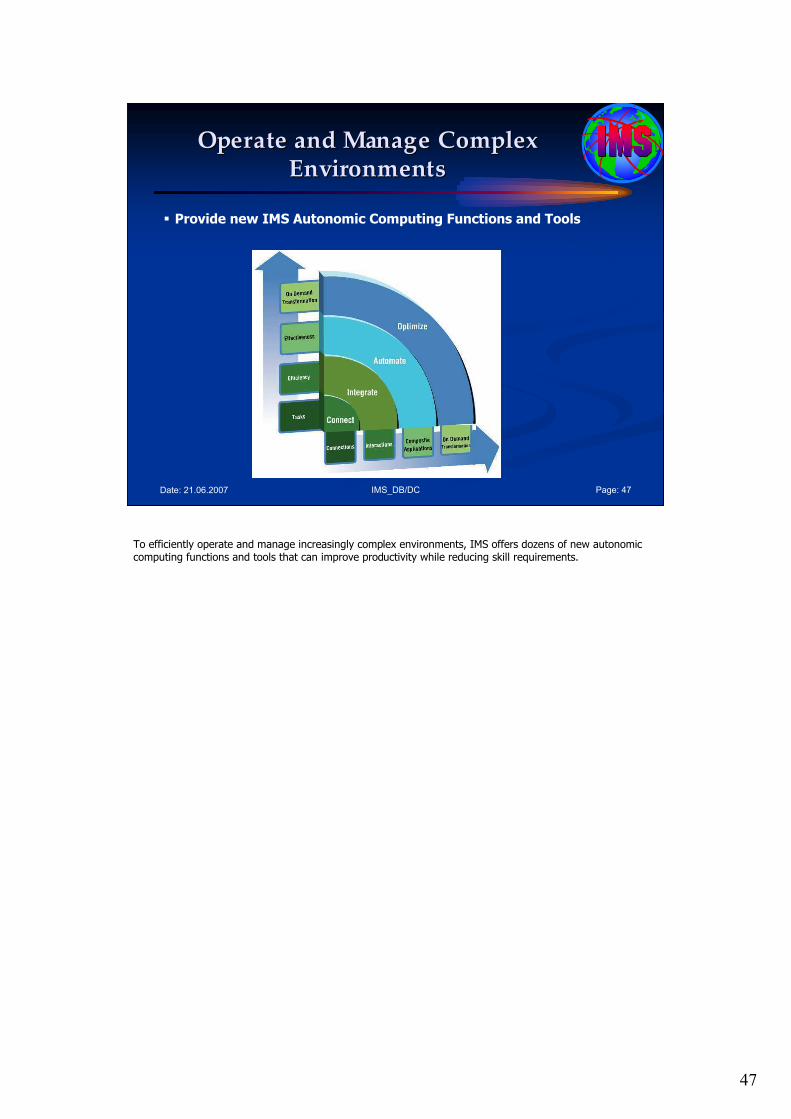
47
IMS_DB/DC Page: 47Date: 21.06.2007
Operate and Manage Complex Operate and Manage Complex
EnvironmentsEnvironments
� Provide new IMS Autonomic Computing Functions and Tools
To efficiently operate and manage increasingly complex environments, IMS offers dozens of new autonomic computing functions and tools that can improve productivity while reducing skill requirements.

48
IMS_DB/DC Page: 48Date: 21.06.2007
Agenda
1. Term of IMS
2. Overview of the IMS product
3. An initial example
4. IMS DB and IMS TM
5. FAQ about TM/DB Basics
6. IMS Usage and Technology Trends
7. Summary
Step 7: Summary of session part I: IMS Overview
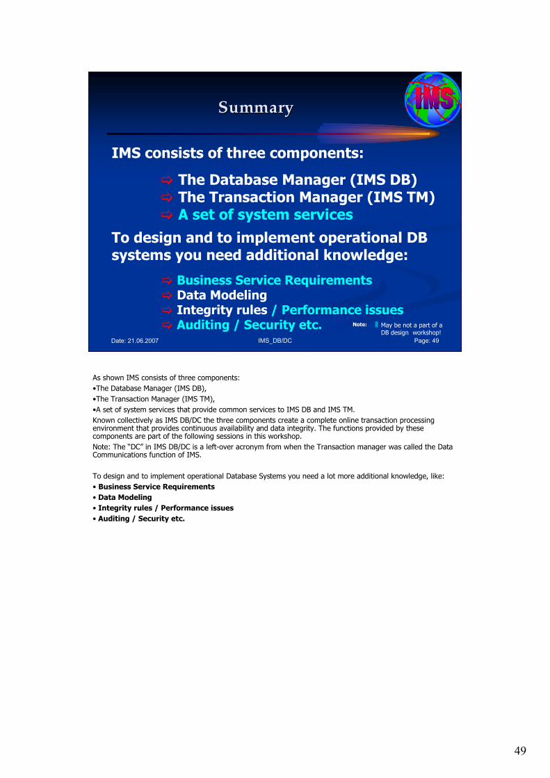
49
IMS_DB/DC Page: 49Date: 21.06.2007
SummarySummary
IMS consists of three components:
� The Database Manager (IMS DB)� The Transaction Manager (IMS TM)� A set of system services
To design and to implement operational DB systems you need additional knowledge:
� Business Service Requirements� Data Modeling� Integrity rules / Performance issues � Auditing / Security etc. May be not a part of a
DB design workshop!
Note:
As shown IMS consists of three components:
•The Database Manager (IMS DB),
•The Transaction Manager (IMS TM),
•A set of system services that provide common services to IMS DB and IMS TM.
Known collectively as IMS DB/DC the three components create a complete online transaction processing environment that provides continuous availability and data integrity. The functions provided by these components are part of the following sessions in this workshop.
Note: The “DC” in IMS DB/DC is a left-over acronym from when the Transaction manager was called the Data Communications function of IMS.
To design and to implement operational Database Systems you need a lot more additional knowledge, like:
• Business Service Requirements
• Data Modeling
• Integrity rules / Performance issues
• Auditing / Security etc.

50
IMS_DB/DC Page: 50Date: 21.06.2007
Source
See: • IBM Web page
http://www-306.ibm.com/software/data/ims/
• BookAn Introduction to IMS, IBM Press
In all sessions I like to motivate you to study additional books and publications about IMS DB/DC.

51
Date: 21.06.2007 IMS_02.ppt Page: 51
Questions / CommentsQuestions / Comments……
? ? ?? ? ?
Questions, comments, further information?
Please feel free to e-mail me!
Dipl.Ing. Werner HoffmannDipl.Ing. Werner Hoffmann
EMAIL: EMAIL: pwhoffmann@[email protected]
The time for this session is over. If you have additional questions or comments or like to get further information please feel free to e mail me at [email protected].

52
IMS_DB/DC Page: 52Date: 21.06.2007
The End…
Part II: IMS Overview
Workshop
The world depends on it
I hope this presentation was right for you! Enjoy the following discussion!
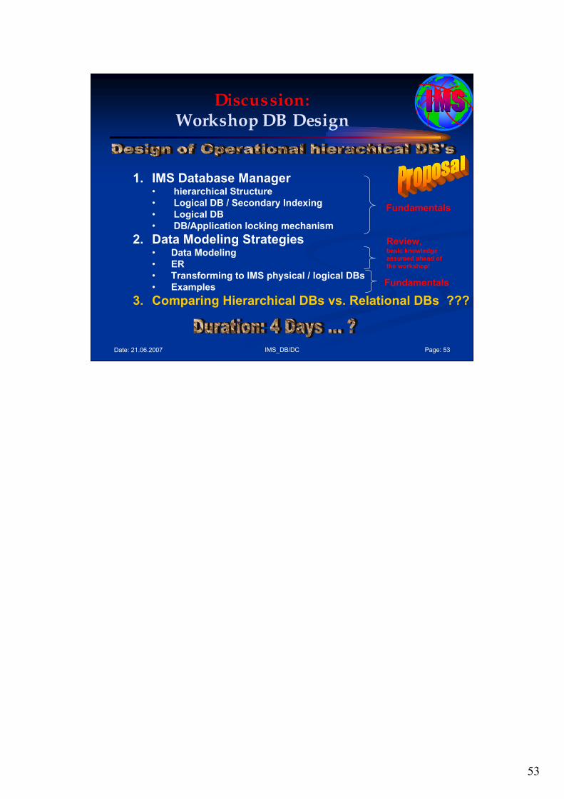
53
IMS_DB/DC Page: 53Date: 21.06.2007
Discussion:Workshop DB Design
1. IMS Database Manager• hierarchical Structure
• Logical DB / Secondary Indexing
• Logical DB
• DB/Application locking mechanism
2. Data Modeling Strategies• Data Modeling
• ER
• Transforming to IMS physical / logical DBs
• Examples
3. Comparing Hierarchical DBs vs. Relational DBs ???
Fundamentals
Fundamentals
Review,basic knowledge
assumed ahead of
the workshop!
1
Date: 21.06.2007 IMS_03._1ppt Page: 1
IBM Mainframe
IMS DB/DC
Database Design Workshop
Part III: Part III:
IMS Hierarchical Database ModelIMS Hierarchical Database ModelSession 1: Initial SessionSession 1: Initial Session
March 2007 March 2007 –– 1st Version1st Version
presented bypresented by
Dipl. Dipl. IngIng. Werner Hoffmann. Werner HoffmannEMAIL: EMAIL: pwhoffmann@[email protected]
A member of IEEE and ACM
Mainframe
Please see the notes pages for additional comments. Please see the notes pages for additional comments.
Welcome to the workshop called “IMS DB/DC". This is part 3: IMS Hierarchical Database Model – Session 1: Initial Session.
Note: This workshop is not a replacement of any of the IBM IMS manuals. And it doesn’t replace any educational staff!
2
IMS_DB/DC Page: 2Date: 21.06.2007
Agenda
IMS Hierarchical Database ModelIMS Hierarchical Database Model
1. Initial Session (this session)
2. Database Basics
3. Hierarchical Access Methods
4. Logical Databases /Logical Relationships
5. Indexed databases
6. Data Sharing Issues
7. Implementing IMS databases
Part III: Sessions
Here is the Agenda for the session Part III: IMS Hierarchical Database Model.

3
Date: 21.06.2007 IMS_03._1ppt Page: 3
Questions / CommentsQuestions / Comments……
? ? ?? ? ?
Questions, comments, further information?
Please feel free to e-mail me!
Dipl.Ing. Werner HoffmannDipl.Ing. Werner Hoffmann
EMAIL: EMAIL: pwhoffmann@[email protected]
The time for this session is over. If you have additional questions or comments or like to get further information please feel free to e mail me at [email protected].

4
IMS_DB/DC Page: 4Date: 21.06.2007
The End…
Part III/1: IMS Hierarchical Database Model IMS Hierarchical Database Model
Initial Session Initial Session
Workshop
The world depends on it
I hope this presentation was right for you! Enjoy the following discussion!
1
Date: 21.06.2007 IMS_03_2.ppt Page: 1
IBM Mainframe
IMS DB/DC
Database Design Workshop
Part III: Part III:
IMS Hierarchical Database ModelIMS Hierarchical Database ModelSession 2: BasicsSession 2: Basics
April 2007 April 2007 –– 2nd Version2nd Version
presented bypresented by
Dipl. Dipl. IngIng. Werner Hoffmann. Werner HoffmannEMAIL: EMAIL: pwhoffmann@[email protected]
A member of IEEE and ACM
Mainframe
Please see the notes pages for additional comments. Please see the notes pages for additional comments.
Welcome to the workshop called “IMS DB/DC". This is part 3: IMS Hierarchical Database Model - Basics.

2
IMS_DB/DC Page: 2Date: 21.06.2007
Agenda Session 2: Database Basics
1. Basic Terms
2. Physical Database
3. Logical Database / Relationships
4. Secondary Indexes
5. How data is stored/retrieved in a DB
6. DB Records, Segments, Pointers
7. Database Segments & Data Area
8. Points not addressed
Here is the Agenda for the IMS DB/DC workshop part III/2: IMS Database Basics.
In this session I like to speak about:
1. Basic Terms
2. Physical Database
3. Logical Database / Relationships
4. Secondary Indexes
5. How data is stored/retrieved in a DB
6. DB Records, Segments, Pointers
7. Database Segments & Data Area
8. Points not addressed.

3
IMS_DB/DC Page: 3Date: 21.06.2007
Agenda Session 2: Database Basics
1. Basic Terms
2. Physical Database
3. Logical Database / Relationships
4. Secondary Indexes
5. How data is stored/retrieved in a DB
6. DB Records, Segments, Pointers
7. Database Segments & Data Area
8. Points not addressed
1. Basic Terms
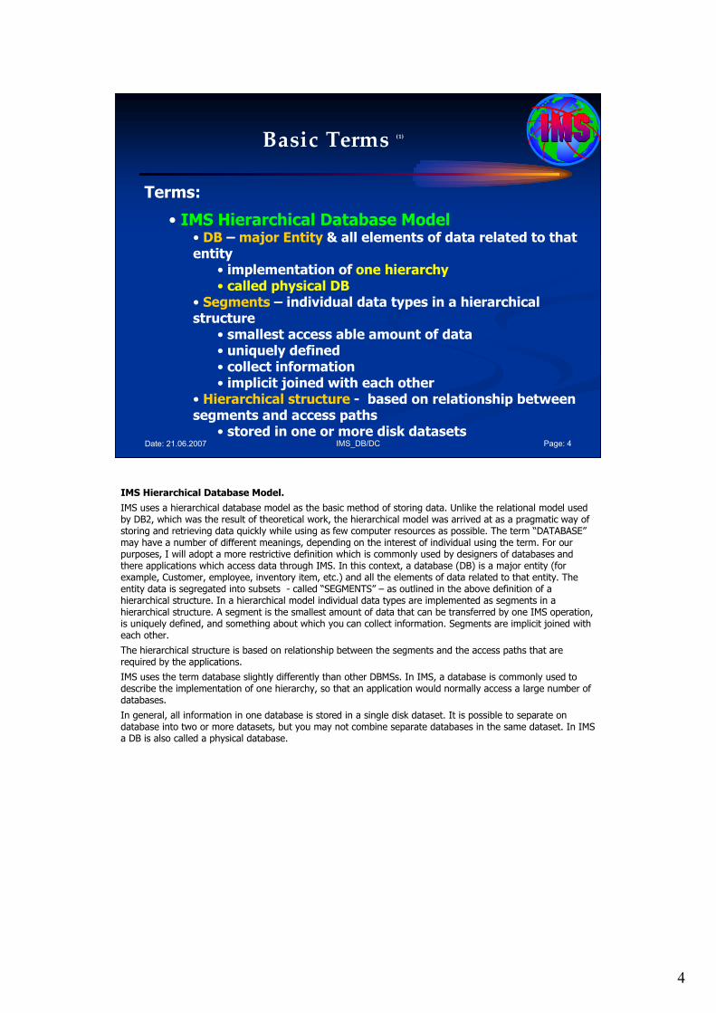
4
IMS_DB/DC Page: 4Date: 21.06.2007
Basic Terms (1)
Terms:
• IMS Hierarchical Database Model• DB – major Entity & all elements of data related to that entity
• implementation of one hierarchy• called physical DB
• Segments – individual data types in a hierarchical structure
• smallest access able amount of data• uniquely defined• collect information• implicit joined with each other
• Hierarchical structure - based on relationship between segments and access paths
• stored in one or more disk datasets
IMS Hierarchical Database Model.
IMS uses a hierarchical database model as the basic method of storing data. Unlike the relational model used by DB2, which was the result of theoretical work, the hierarchical model was arrived at as a pragmatic way of storing and retrieving data quickly while using as few computer resources as possible. The term “DATABASE”may have a number of different meanings, depending on the interest of individual using the term. For our purposes, I will adopt a more restrictive definition which is commonly used by designers of databases and there applications which access data through IMS. In this context, a database (DB) is a major entity (for example, Customer, employee, inventory item, etc.) and all the elements of data related to that entity. The entity data is segregated into subsets - called “SEGMENTS” – as outlined in the above definition of a hierarchical structure. In a hierarchical model individual data types are implemented as segments in a hierarchical structure. A segment is the smallest amount of data that can be transferred by one IMS operation, is uniquely defined, and something about which you can collect information. Segments are implicit joined with each other.
The hierarchical structure is based on relationship between the segments and the access paths that are required by the applications.
IMS uses the term database slightly differently than other DBMSs. In IMS, a database is commonly used to describe the implementation of one hierarchy, so that an application would normally access a large number of databases.
In general, all information in one database is stored in a single disk dataset. It is possible to separate on database into two or more datasets, but you may not combine separate databases in the same dataset. In IMS a DB is also called a physical database.
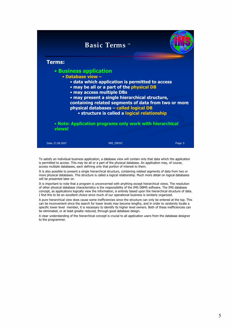
5
IMS_DB/DC Page: 5Date: 21.06.2007
Basic Terms (2)
Terms:
• Business application• Database view –
• data which application is permitted to access• may be all or a part of the physical DB• may access multiple DBs• may present a single hierarchical structure, containing related segments of data from two or more physical databases – called logical DB
• structure is called a logical relationship
• Note: Application programs only work with hierarchical views!
To satisfy an individual business application, a database view will contain only that data which the application is permitted to access. This may be all or a part of the physical database. An application may, of course, access multiple databases, each defining only that portion of interest to them.
It is also possible to present a single hierarchical structure, containing related segments of data from two or more physical databases. This structure is called a logical relationship. Much more detail on logical databases will be presented later on.
It is important to note that a program is unconcerned with anything except hierarchical views. The resolution of other physical database characteristics is the responsibility of the IMS DBMS software. The IMS database concept, as applications logically view the information, is entirely based upon the hierarchical structure of data. I find this to be an excellent choice since much of our operational business is similarly organized.
A pure hierarchical view does cause some inefficiencies since the structure can only be entered at the top. This can be inconvenient since the search for lower levels may become lengthy, and in order to randomly locate a specific lower level member, it is necessary to identify its higher level owners. Both of these inefficiencies can be eliminated, or at least greatly reduced, through good database design.
A clear understanding of the hierarchical concept is crucial to all application users from the database designer to the programmer.

6
IMS_DB/DC Page: 6Date: 21.06.2007
Agenda Session 2: Database Basics
1. Basic Terms
2. Physical Database
3. Logical Database / Relationships
4. Secondary Indexes
5. How data is stored/retrieved in a DB
6. DB Records, Segments, Pointers
7. Database Segments & Data Area
8. Points not addressed
2. Physical Database
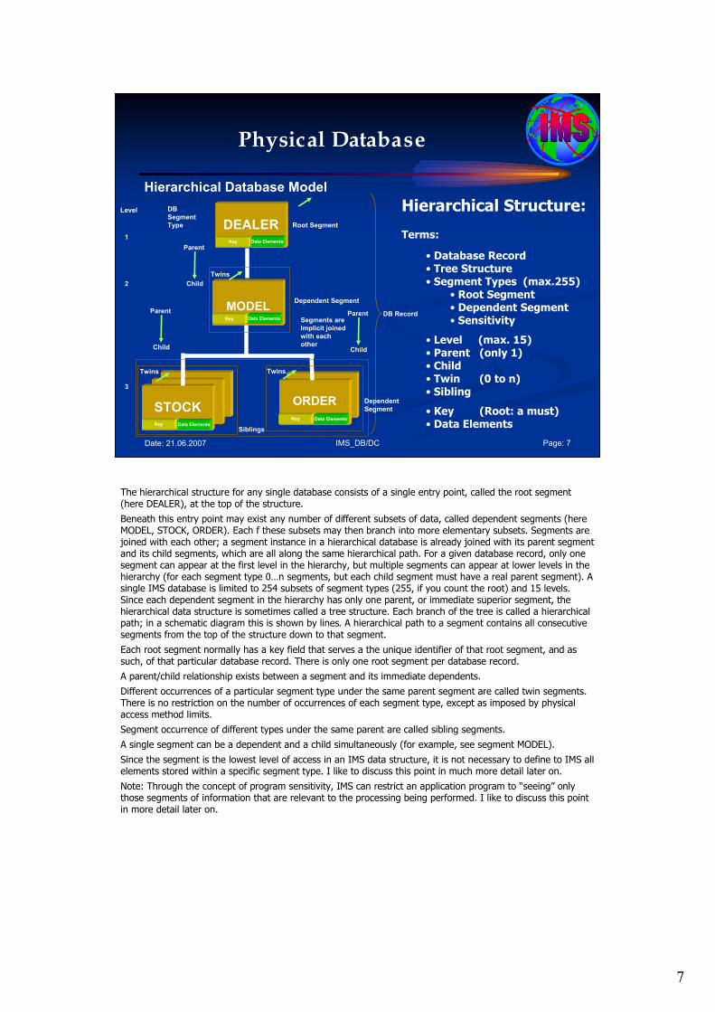
7
IMS_DB/DC Page: 7Date: 21.06.2007
Physical Database
Hierarchical Structure:
Terms:
• Database Record• Tree Structure• Segment Types (max.255)
• Root Segment• Dependent Segment• Sensitivity
• Level (max. 15)• Parent (only 1)• Child• Twin (0 to n) • Sibling
• Key (Root: a must)• Data Elements
ORDERSTOCKSTOCK
DEALER
STOCK
MODEL
ORDER
Hierarchical Database Model
Level
1
2
3
Parent
Child
Twins
DB
Segment
Type
Segments are
Implicit joined
with each
other
Siblings
Root Segment
Dependent Segment
Key
Key
Key
Key
DB Record
Dependent
Segment
Twins
Twins
Data Elements
Data Elements
Data Elements
Data Elements
Parent
Child
Parent
Child
The hierarchical structure for any single database consists of a single entry point, called the root segment (here DEALER), at the top of the structure.
Beneath this entry point may exist any number of different subsets of data, called dependent segments (here MODEL, STOCK, ORDER). Each f these subsets may then branch into more elementary subsets. Segments are joined with each other; a segment instance in a hierarchical database is already joined with its parent segment and its child segments, which are all along the same hierarchical path. For a given database record, only one segment can appear at the first level in the hierarchy, but multiple segments can appear at lower levels in the hierarchy (for each segment type 0…n segments, but each child segment must have a real parent segment). A single IMS database is limited to 254 subsets of segment types (255, if you count the root) and 15 levels. Since each dependent segment in the hierarchy has only one parent, or immediate superior segment, the hierarchical data structure is sometimes called a tree structure. Each branch of the tree is called a hierarchical path; in a schematic diagram this is shown by lines. A hierarchical path to a segment contains all consecutive segments from the top of the structure down to that segment.
Each root segment normally has a key field that serves a the unique identifier of that root segment, and as such, of that particular database record. There is only one root segment per database record.
A parent/child relationship exists between a segment and its immediate dependents.
Different occurrences of a particular segment type under the same parent segment are called twin segments. There is no restriction on the number of occurrences of each segment type, except as imposed by physical access method limits.
Segment occurrence of different types under the same parent are called sibling segments.
A single segment can be a dependent and a child simultaneously (for example, see segment MODEL).
Since the segment is the lowest level of access in an IMS data structure, it is not necessary to define to IMS all elements stored within a specific segment type. I like to discuss this point in much more detail later on.
Note: Through the concept of program sensitivity, IMS can restrict an application program to “seeing” only those segments of information that are relevant to the processing being performed. I like to discuss this point in more detail later on.
8
IMS_DB/DC Page: 8Date: 21.06.2007
Agenda Session 2: Database Basics
1. Basic Terms
2. Physical Database
3. Logical Database / Relationships
4. Secondary Indexes
5. How data is stored/retrieved in a DB
6. DB Records, Segments, Pointers
7. Database Segments & Data Area
8. Points not addressed
3. Logical Database / Relationships
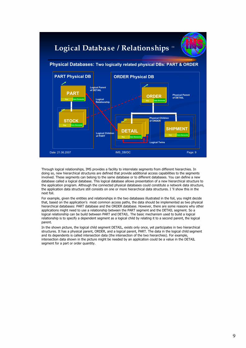
9
IMS_DB/DC Page: 9Date: 21.06.2007
Logical Database / Relationships (1)
STOCKSTOCKDETAIL
ORDER
SHIPMENT
Key
Key
Key
Data Elements
Data Elements
Data Elements
ORDER Physical DB
Physical Children
of ORDER
Physical Parent
of DETAIL
Physical Databases: Two logically related physical DBs: PART & ORDER
PARTKey Data Elements
STOCKKey Data Elements
PART Physical DB
Logical
Relationship
Logical Parent
of DETAIL
Logical Children
of PART
Logical Twins
Through logical relationships, IMS provides a facility to interrelate segments from different hierarchies. In doing so, new hierarchical structures are defined that provide additional access capabilities to the segments involved. These segments can belong to the same database or to different databases. You can define a new database called a logical database. This logical database allows presentation of a new hierarchical structure to the application program. Although the connected physical databases could constitute a network data structure, the application data structure still consists on one or more hierarchical data structures. I ‘ll show this in the next foil.
For example, given the entities and relationships in the two databases illustrated in the foil, you might decide that, based on the application’s most common access paths, the data should be implemented as two physical hierarchical databases: PART database and the ORDER database. However, there are some reasons why other applications might need to use a relationship between the PART segment and the DETAIL segment. So a logical relationship can be build between PART and DETAIL. The basic mechanism used to build a logical relationship is to specify a dependent segment as a logical child by relating it to a second parent, the logical parent.
In the shown picture, the logical child segment DETAIL, exists only once, yet participates in two hierarchical structures. It has a physical parent, ORDER, and a logical parent, PART. The data in the logical child segment and its dependents is called intersection data (the intersection of the two hierarchies). For example, intersection data shown in the picture might be needed by an application could be a value in the DETAIL segment for a part or order quantity.
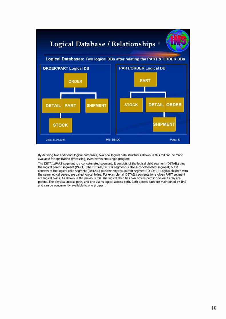
10
IMS_DB/DC Page: 10Date: 21.06.2007
Logical Database / Relationships (2)
Logical Databases: Two logical DBs after relating the PART & ORDER DBs
DETAIL PART
ORDER
SHIPMENT
ORDER/PART Logical DB
STOCK
DETAIL ORDER
PART
STOCK
PART/ORDER Logical DB
SHIPMENT
By defining two additional logical databases, two new logical data structures shown in this foil can be made available for application processing, even within one single program.
The DETAIL/PART segment is a concatenated segment. It consists of the logical child segment (DETAIL) plus the logical parent segment (PART). The DETAIL/ORDER segment is also a concatenated segment, but it consists of the logical child segment (DETAIL) plus the physical parent segment (ORDER). Logical children with the same logical parent are called logical twins. For example, all DETAIL segments for a given PART segment are logical twins. As shown in the previous foil. The logical child has two access paths: one via its physical parent, The physical access path, and one via its logical access path. Both access path are maintained by IMS and can be concurrently available to one program.
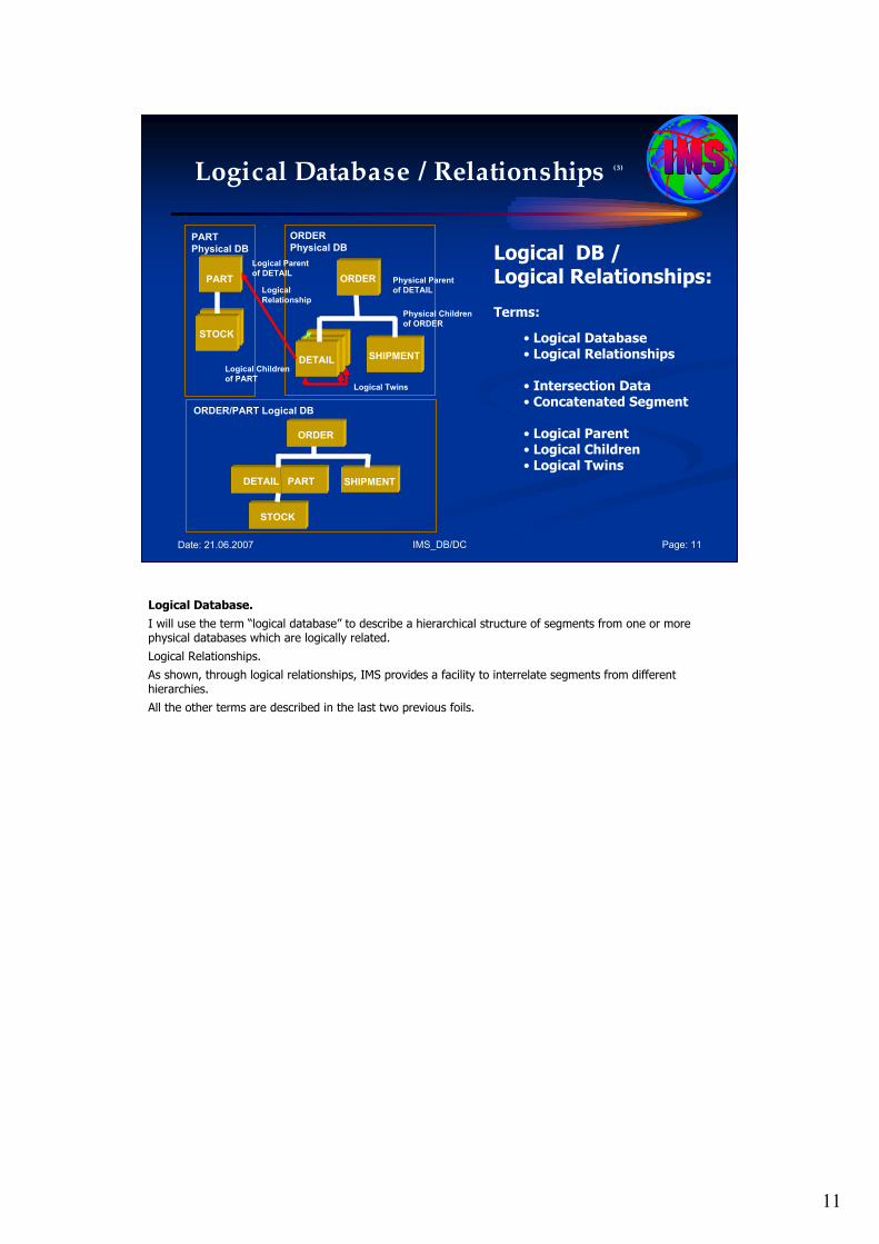
11
IMS_DB/DC Page: 11Date: 21.06.2007
Logical Database / Relationships (3)
Logical DB /Logical Relationships:
Terms:
• Logical Database• Logical Relationships
• Intersection Data• Concatenated Segment
• Logical Parent• Logical Children• Logical Twins
PART
DETAIL
ORDER
SHIPMENT
STOCK
PART
Physical DB
ORDER
Physical DB
Logical
Relationship
Logical Parent
of DETAIL
Logical Children
of PART
Physical Children
of ORDER
Physical Parent
of DETAIL
Logical Twins
DETAIL PART
ORDER
SHIPMENT
ORDER/PART Logical DB
STOCK
Logical Database.
I will use the term “logical database” to describe a hierarchical structure of segments from one or more physical databases which are logically related.
Logical Relationships.
As shown, through logical relationships, IMS provides a facility to interrelate segments from different hierarchies.
All the other terms are described in the last two previous foils.
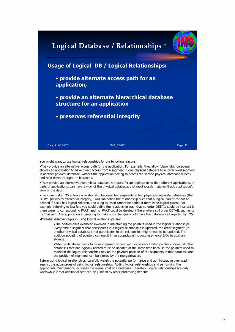
12
IMS_DB/DC Page: 12Date: 21.06.2007
Logical Database / Relationships (4)
Usage of Logical DB / Logical Relationships:
• provide alternate access path for an application,
• provide an alternate hierarchical database structure for an application
• preserves referential integrity
You might want to use logical relationships for the following reasons:
•They provide an alternative access path for the application. For example, they allow (depending on pointer choice) an application to have direct access from a segment in one physical database to a lower level segment in another physical database, without the application having to access the second physical database directly and read down through the hierarchy.
•They provide an alternative hierarchical database structure for an application so that different applications, or parts of applications, can have a view of the physical databases that most closely matches that’s application’s view of the data.
•They can make IMS enforce a relationship between two segments in two physically separate databases (that is, IMS preserves referential integrity). You can define the relationship such that a logical parent cannot be deleted if it still has logical children, and a logical child cannot be added if there is no logical parent. For example, referring to last foil, you could define the relationship such that no order DETAIL could be inserted it there were no corresponding PART, and no PART could be deleted if there where still order DETAIL segments for that part. Any application attempting to make such changes would have the database call rejected by IMS.
•Potential disadvantages in using logical relationships are:
•The performance overhead involved in maintaining the pointers used in the logical relationships. Every time a segment that participates in a logical relationship is updated, the other segment (in another physical database) that participates in the relationship might need to be updated. The addition updating of pointers can result in an appreciable increase in physical I/Os to auxiliary storage.
•When a database needs to be reorganized, except with some very limited pointer choices, all other databases that are logically related must be updated at the same time because the pointers used to maintain the logical relationships rely on the physical position of the segments in that database and the position of segments can be altered by the reorganization.
Before using logical relationships, carefully weigh the potential performance and administrative overhead against the advantages of using logical relationships. Adding logical relationships and performing the appropriate maintenance increases the overall cost of a database. Therefore, logical relationships are only worthwhile if that additional cost can be justified by other processing benefits.
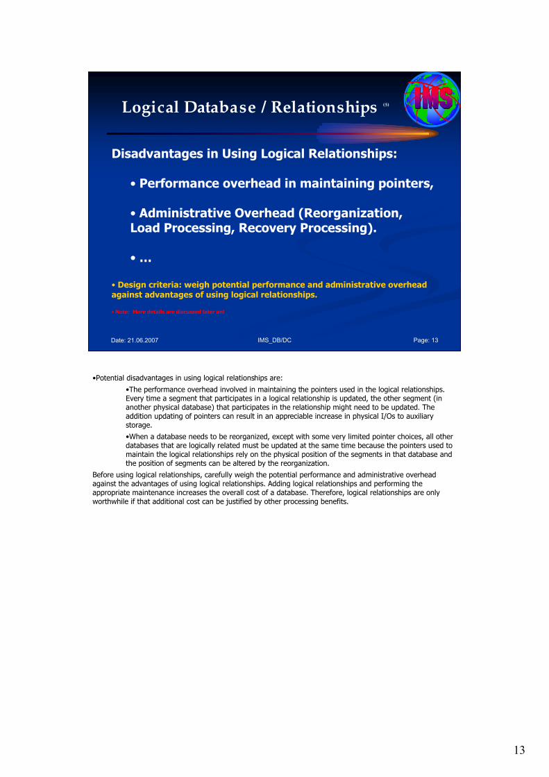
13
IMS_DB/DC Page: 13Date: 21.06.2007
Logical Database / Relationships (5)
Disadvantages in Using Logical Relationships:
• Performance overhead in maintaining pointers,
• Administrative Overhead (Reorganization, Load Processing, Recovery Processing).
•…
• Design criteria: weigh potential performance and administrative overhead against advantages of using logical relationships.
• Note: More details are discussed later on!
•Potential disadvantages in using logical relationships are:
•The performance overhead involved in maintaining the pointers used in the logical relationships. Every time a segment that participates in a logical relationship is updated, the other segment (in another physical database) that participates in the relationship might need to be updated. The addition updating of pointers can result in an appreciable increase in physical I/Os to auxiliary storage.
•When a database needs to be reorganized, except with some very limited pointer choices, all other databases that are logically related must be updated at the same time because the pointers used to maintain the logical relationships rely on the physical position of the segments in that database and the position of segments can be altered by the reorganization.
Before using logical relationships, carefully weigh the potential performance and administrative overhead against the advantages of using logical relationships. Adding logical relationships and performing the appropriate maintenance increases the overall cost of a database. Therefore, logical relationships are only worthwhile if that additional cost can be justified by other processing benefits.
14
IMS_DB/DC Page: 14Date: 21.06.2007
Agenda Session 2: Database Basics
1. Basic Terms
2. Physical Database
3. Logical Database / Relationships
4. Secondary Indexes
5. How data is stored/retrieved in a DB
6. DB Records, Segments, Pointers
7. Database Segments & Data Area
8. Points not addressed
4. Secondary Indexes

15
IMS_DB/DC Page: 15Date: 21.06.2007
Secondary Indexes (1)
Segments used for
Secondary Indexes:
Terms:
• Target Segment• Source Segment• Pointer Segment
• Sparse Indexing
• secondary index key -> search field
• max. 32 Sec.IX/segment type• max. 1000 Sec.IX/DB• Sec.IX key: 1..5 fields from the index source field
Pointer
Segment
Secondary Index
DB
Sec.IX
DB
Ordered by Sec.IX key
Key:
Unique
/SX
/CX
or
not unique
value
Target
Segment
Source
Segment
A Root or
dependent
segment
type
Same segment
type as the
target segment
type or, as shown,
a dependent of the
target segment
type
Physical or
Logical DB
IMS DB
Order dependent
on access method
Indexed
DB
The content of specified
fields in each source
segment is duplicated
in the respective pointer
segment.
IMS provides additional access flexibility with secondary index databases. A secondary index represents a different access path (pointers) to any segment in the database other tha the path defined by the key field in the root segment. The additional access paths can result in faster retrieval of data. A secondary index is in its own separate database.
There can be 32 secondary indexes for a segment type and a total of 1000 secondary indexes for a single database.
To setup a secondary index, three types of segments must be defined to IMS: a pointer segment, a target segment, and a source segment.
After an index is defined, IMS automatically maintains the index if the data on which the index relies changes, even if the program causing that change is not aware of the index.
Pointer Segment.
The pointer segment is contained in the secondary index database and is the only type of segment in the secondary index database.
Target segment.
The index target segment is the segment that becomes initially accessible from the secondary index. The target segment:
•Is the segment that the application program needs to view as a root in a hierarchy.
•Is in the database that is being indexed.
•Is pointed to by the pointer segment.
•Can be at any one of the 15 levels in the database.
•Is accessed directly using the RBA or symbolic pointer stored in the pointer segment.
The database being indexed can be a physical or logical database. Quit often, the target segment is the root segment.
Source Segment.
The source segment is also in the regular database. The source segment contains the field (or fields) that the pointer segment has as its key field. Data is copied from the source segment and put in the pointer segment’s key field. The source and the target segment can be the same segment, or the source segment can be a dependent of the target segment.
The pointer segments are ordered and accessed based on the field contents of the index source segment. In general, there is one index pointer segment for each index source segment, but multiple index pointer segments can point to the same index target segment. The index source and index target segment might be the same, or the index source segment might be a dependent of the index target segment.
The secondary index key (search field) is made up of one to five fields from the index source segment. The search field does not have to be a unique value, but I strongly recommends you make it a unique value to avoid the overhead in storing and searching duplicates. There are a number of fields that can be concatenated to the end of the secondary index search field to make it unique:
•A subsequence field, consisting of one to five more fields from the index source segment. This is maintained by IMS but, unlike the search field, cannot be used by an application for a search argument when using the secondary index.
•A system defined field that uniquely defines the index source segment: the /SX variable.
•A system defined field that defines the concatenated key (the concatenation of the key values of all of the segment occurrences in the hierarchical path leading to that segment) of the index source segment: the /CX variable.
Sparse Indexing.
Another technique that can be used with secondary indexes is sparse indexing. Normally IMS maintains index entries for all occurrences of the secondary index source segment. However, it is possible to cause IMS suppress index entries for some of the occurrences of the index source segment. You may want to suppress index entries if you were only interested in processing segments that had a non-null value in the field. As a general rule, only consider this technique if you expect 205 or less of the index source segments to be created. The suppression can be done either by specifying that all bytes in the field should be a specific character (NULLVAL parameter) or by selection with the Secondary index Maintenance exit routine.
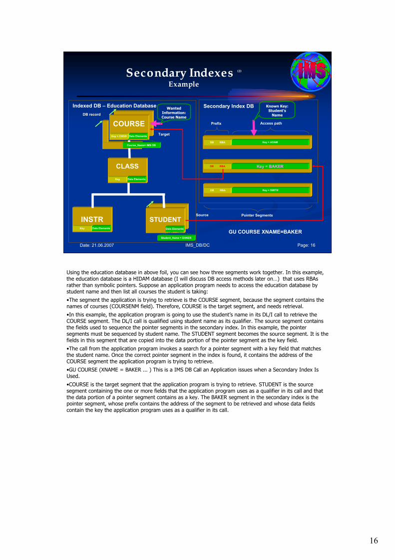
16
IMS_DB/DC Page: 16Date: 21.06.2007
Secondary Indexes (2)
Example
GU COURSE XNAME=BAKERKey= S0222
Prefix
DB RBA Key = ADAM
DB RBA Key = BAKER
DB RBA Key = SMITH
Pointer Segments
Secondary Index DB
Access pathCOURSE
CLASS
INSTR STUDENT
Indexed DB – Education Database
DB record
Key = C0020 Data Elements
Key Data Elements
Key Data Elements Data Elements
Known Key:Student’s Name
Wanted Information:Course Name
Course_Name= IMS DB
Target
Source
Student_Name = BAKER
Using the education database in above foil, you can see how three segments work together. In this example, the education database is a HIDAM database (I will discuss DB access methods later on…) that uses RBAsrather than symbolic pointers. Suppose an application program needs to access the education database by student name and then list all courses the student is taking:
•The segment the application is trying to retrieve is the COURSE segment, because the segment contains the names of courses (COURSENM field). Therefore, COURSE is the target segment, and needs retrieval.
•In this example, the application program is going to use the student’s name in its DL/I call to retrieve the COURSE segment. The DL/I call is qualified using student name as its qualifier. The source segment contains the fields used to sequence the pointer segments in the secondary index. In this example, the pointer segments must be sequenced by student name. The STUDENT segment becomes the source segment. It is the fields in this segment that are copied into the data portion of the pointer segment as the key field.
•The call from the application program invokes a search for a pointer segment with a key field that matches the student name. Once the correct pointer segment in the index is found, it contains the address of the COURSE segment the application program is trying to retrieve.
•GU COURSE (XNAME = BAKER ... ) This is a IMS DB Call an Application issues when a Secondary Index Is Used.
•COURSE is the target segment that the application program is trying to retrieve. STUDENT is the source segment containing the one or more fields that the application program uses as a qualifier in its call and that the data portion of a pointer segment contains as a key. The BAKER segment in the secondary index is the pointer segment, whose prefix contains the address of the segment to be retrieved and whose data fields contain the key the application program uses as a qualifier in its call.
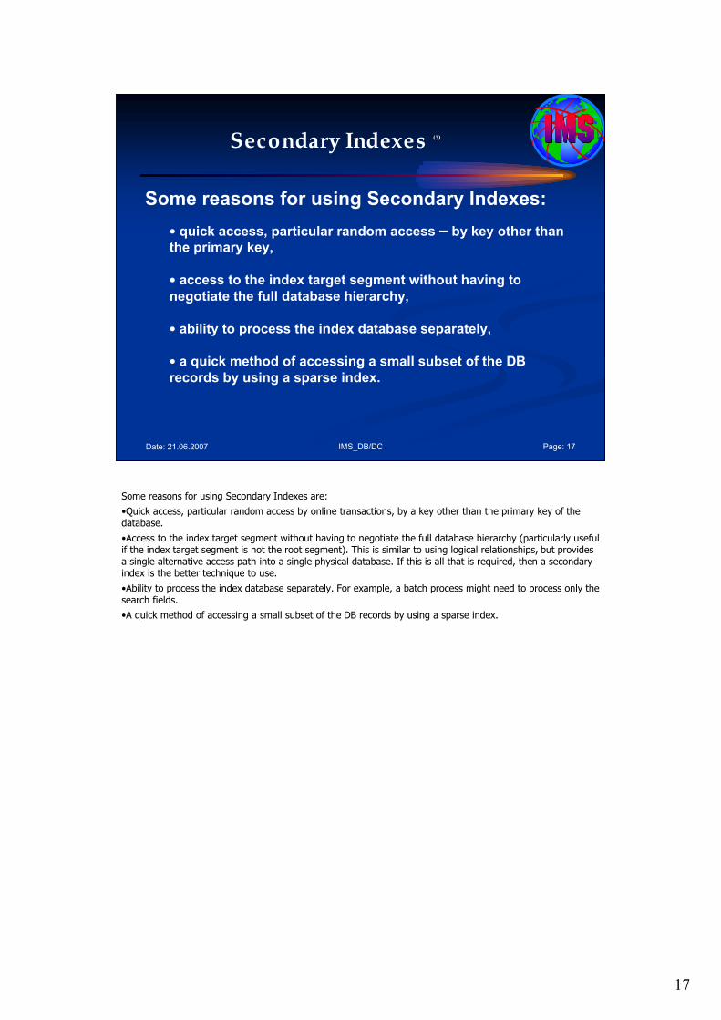
17
IMS_DB/DC Page: 17Date: 21.06.2007
Secondary Indexes (3)
Some reasons for using Secondary Indexes:
• quick access, particular random access – by key other than the primary key,
• access to the index target segment without having to negotiate the full database hierarchy,
• ability to process the index database separately,
• a quick method of accessing a small subset of the DB records by using a sparse index.
Some reasons for using Secondary Indexes are:
•Quick access, particular random access by online transactions, by a key other than the primary key of the database.
•Access to the index target segment without having to negotiate the full database hierarchy (particularly useful if the index target segment is not the root segment). This is similar to using logical relationships, but provides a single alternative access path into a single physical database. If this is all that is required, then a secondary index is the better technique to use.
•Ability to process the index database separately. For example, a batch process might need to process only the search fields.
•A quick method of accessing a small subset of the DB records by using a sparse index.

18
IMS_DB/DC Page: 18Date: 21.06.2007
Secondary Indexes (4)
Disadvantages in using Secondary Indexes:
• the performance overheads in updating the secondary index DB,
• the administrative overheads in setting up, monitoring, backing up, and tuning the secondary index DB,
• when the database containing the index source segment is reorganized, the secondary index must also be rebuilt.
• Design criteria: weigh potential performance and administrative overhead against advantages of using Secondary Indexes.
• Note: More details are discussed later on!
Potential disadvantages in using Secondary Indexes are:
•The performance overheads in updating the secondary index database every time any of the fields making up search field in the index source segment is updated or when the index source segment is inserted or deleted.
•The administrative overheads in setting up, monitoring, backing up, and tuning the secondary index database.
•When the database containing the index source segment is reorganized, the secondary index must also be rebuilt because the pointers used to maintain the connection between the source segment and the secondary index rely on the physical position of the source segment in the database, which can be altered by the reorganization.
As with logical relationships, consider carefully whether the benefits of using a secondary index outweigh the performance and administrative overhead.
19
IMS_DB/DC Page: 19Date: 21.06.2007
Agenda Session 2: Database Basics
1. Basic Terms
2. Physical Database
3. Logical Database / Relationships
4. Secondary Indexes
5. How data is stored/retrieved in a DB
6. DB Records, Segments, Pointers
7. Database Segments & Data Area
8. Points not addressed
5. How data is stored/retrieved in a DB
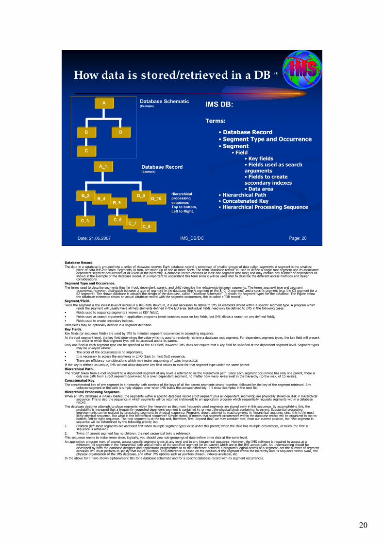
20
IMS_DB/DC Page: 20Date: 21.06.2007
How data is stored/retrieved in a DB (1)
A
B
C
D
Database Schematic(Example)
D_10
C_8C_7
B_5B_4
A_1
B_2
C_3
D_9
C_6
Database Record(Example)
Hierarchical
processing
sequence:
Top to bottom,
Left to Right.
IMS DB:
Terms:
• Database Record• Segment Type and Occurrence• Segment
• Field• Key fields• Fields used as search arguments• Fields to create secondary indexes• Data area
• Hierarchical Path• Concatenated Key• Hierarchical Processing Sequence
Database Record.
The data in a database is grouped into a series of database records. Each database record is composed of smaller groups of data called segments. A segment is the smallest piece of data IMS can store. Segments, in turn, are made up of one or more fields. The term “database record” is used to define a single root segment and its associated dependent segment occurrences at all levels in the hierarchy. A database record contains at least one segment (the root) and may contain any number of dependents as shown in the example of the database record. It is important to understand this term since it will be used later to describe the different access methods and design considerations.
Segment Type and Occurrence.
The terms used to describe segments thus far (root, dependent, parent, and child) describe the relationship between segments. The terms segment type and segment occurrence, however, distinguish between a type of segment in the database (the A segment or the B, C, D segment) and a specific segment (e.g. the C3 segment for a B2 segment). The shown database is actually the design of the database, called “Database Schematic”. It shows the segment types for the database. The Figure below the database schematic shows an actual database record with the segment occurrences, this is called a “DB record”.
Segment/Field.
Since the segment is the lowest level of access in a IMS data structure, it is not necessary to define to IMS all elements stored within a specific segment type. A program which reads the segment will usually have all field elements defined in the I/O area. Individual fields need only be defined to IMS in the following cases:
• Fields used to sequence segments ( known as KEY fields),
• Fields used as search arguments in application programs (most searches occur on key fields, but IMS allows a search on any defined field),
• Fields used to create secondary indexes.
Data fields may be optionally defined in a segment definition.
Key Fields.
Key fields (or sequence fields) are used by IMS to maintain segment occurrences in ascending sequence.
At the root segment level, the key field determines the value which is used to randomly retrieve a database root segment. For dependent segment types, the key field will present the order in which that segment type will be accessed under its parent.
Only one field in each segment type can be specified as the KEY field, however, IMS does not require that a key field be specified at the dependent segment level. Segment types may be unkeyed where:
• The order of the occurrences is no importance,
• It is necessary to access the segments in LIFO (Last In, First Out) sequence,
• There are efficiency considerations which may make sequencing of twins impractical.
If the key is defined as unique, IMS will not allow duplicate key field values to exist for that segment type under the same parent.
Hierarchical Path.
The “road” taken from a root segment to a dependent segment at any level is referred to as the hierarchical path. Since each segment occurrence has only one parent, there is only one path from a root segment downward to a given dependant segment, no matter how many levels exist in the hierarchy (to the max. of 15 levels).
Concatenated Key.
The concatenated key of any segment in a hierarchy path consists of the keys of all the parent segments strung together, followed by the key of the segment retrieved. Any unkeyed segment in the path is simply skipped over when IMS builds the concatenated key. I ‘ll show examples in the next foil.
Hierarchical Processing Sequence.
When an IMS database is initially loaded, the segments within a specific database record (root segment plus all dependent segments) are physically stored on disk in hierarchical sequence. This is also the sequence in which segments will be returned (retrieved) to an application program which sequentially requests segments within a database record.
The database designer attempts to place segments within the hierarchy so that most frequently used segments are stored early in this sequence. By accomplishing this, the probability is increased that a frequently requested dependent segment is contained in, or near, the physical block containing its parent. Substantial processing improvements can be realized by processing segments in physical sequence. Programs should attempt to read segments in hierarchical sequence since this is the most likely physical sequence. But what is this hierarchical sequence? Simple stated, it means that segment occurrences within the database record will be organized in top-to-bottom, left-to-right sequence. The root segment is at the top and, therefore, first. Beyond that, we may consider that, from our current position, the next segment in sequence will be determined by the following priority list:
1. Children (left-most segments are accessed first when multiple segment types exist under this parent; when the child has multiple occurrences, or twins, the first in sequence is retrieved).
2. Twins (if current segment has no children, the next sequential twin is retrieved).
This sequence seems to make sense since, logically, you should view sub groupings of data before other data at the same level.
An application program may, of course, access specific segment types at any level and in any hierarchical sequence. However, the IMS software is required to access at a minimum, all segments in the hierarchical path and all twins of the specified segment (or its parent) which are in the IMS access path. An understanding should be developed by both the database designer and applications programmer as to the difference between a program’s logical access of a segment, ant the number of segment accesses IMS must perform to satisfy that logical function. This difference is based on the position of the segment within the hierarchy and its sequence within twins, the physical organization of the IMS database, and other IMS options such as pointers chosen, indexes available, etc.
In the above foil I have shown alphanumeric IDs for a database schematic and for a specific database record with its segment occurrences.
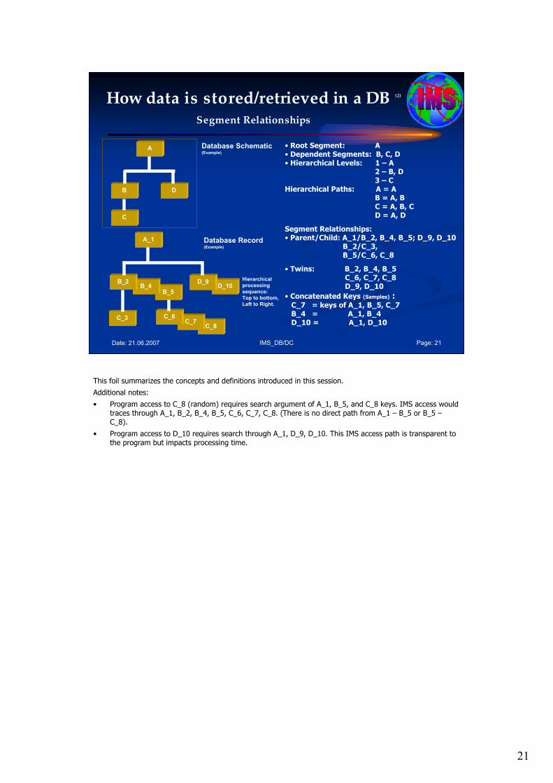
21
IMS_DB/DC Page: 21Date: 21.06.2007
How data is stored/retrieved in a DB (2)
Segment Relationships
A
B
C
D
Database Schematic(Example)
D_10
C_8C_7
B_5B_4
A_1
B_2
C_3
D_9
C_6
Database Record(Example)
Hierarchical
processing
sequence:
Top to bottom,
Left to Right.
• Root Segment: A• Dependent Segments: B, C, D• Hierarchical Levels: 1 – A
2 – B, D3 – C
Hierarchical Paths: A = AB = A, BC = A, B, CD = A, D
Segment Relationships:• Parent/Child: A_1/B_2, B_4, B_5; D_9, D_10
B_2/C_3,B_5/C_6, C_8
• Twins: B_2, B_4, B_5C_6, C_7, C_8D_9, D_10
• Concatenated Keys (Samples) :C_7 = keys of A_1, B_5, C_7B_4 = A_1, B_4D_10 = A_1, D_10
This foil summarizes the concepts and definitions introduced in this session.
Additional notes:
• Program access to C_8 (random) requires search argument of A_1, B_5, and C_8 keys. IMS access would traces through A_1, B_2, B_4, B_5, C_6, C_7, C_8. (There is no direct path from A_1 – B_5 or B_5 –C_8).
• Program access to D_10 requires search through A_1, D_9, D_10. This IMS access path is transparent to the program but impacts processing time.
22
IMS_DB/DC Page: 22Date: 21.06.2007
Agenda Session 2: Database Basics
1. Basic Terms
2. Physical Database
3. Logical Database / Relationships
4. Secondary Indexes
5. How data is stored/retrieved in a DB
6. DB Records, Segments, Pointers
7. Database Segments & Data Area
8. Points not addressed
6. DB Records, Segments, Pointers
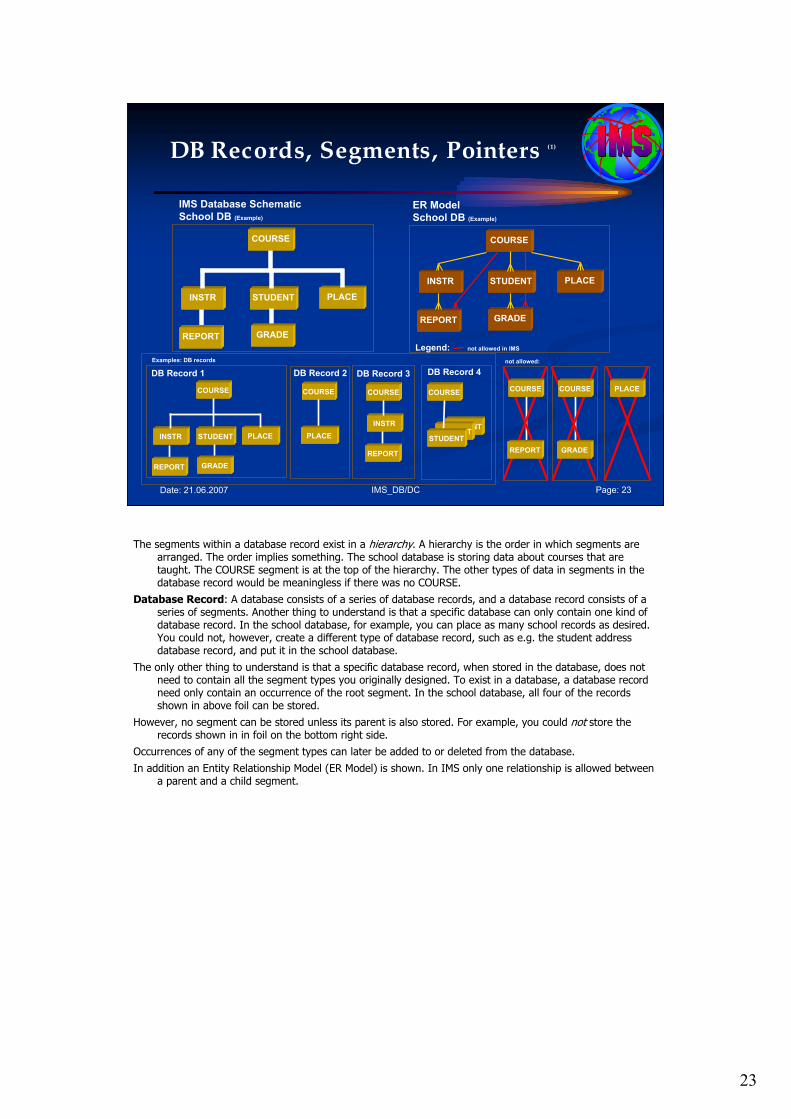
23
IMS_DB/DC Page: 23Date: 21.06.2007
DB Records, Segments, Pointers (1)
COURSE
INSTR STUDENT
IMS Database Schematic
School DB (Example)
PLACE
REPORT GRADE
COURSE
INSTR STUDENT PLACE
REPORT GRADE
ER Model
School DB (Example)
Legend: not allowed in IMS
PLACECOURSE
GRADE
COURSE
REPORT
not allowed:
STUDENTSTUDENT
COURSE
INSTR STUDENT PLACE
REPORT GRADE
COURSE
PLACE
COURSE
INSTR
REPORT
COURSE
STUDENT
DB Record 1 DB Record 2 DB Record 3 DB Record 4
Examples: DB records
The segments within a database record exist in a hierarchy. A hierarchy is the order in which segments are arranged. The order implies something. The school database is storing data about courses that are taught. The COURSE segment is at the top of the hierarchy. The other types of data in segments in the database record would be meaningless if there was no COURSE.
Database Record: A database consists of a series of database records, and a database record consists of a series of segments. Another thing to understand is that a specific database can only contain one kind of database record. In the school database, for example, you can place as many school records as desired. You could not, however, create a different type of database record, such as e.g. the student address database record, and put it in the school database.
The only other thing to understand is that a specific database record, when stored in the database, does not need to contain all the segment types you originally designed. To exist in a database, a database record need only contain an occurrence of the root segment. In the school database, all four of the records shown in above foil can be stored.
However, no segment can be stored unless its parent is also stored. For example, you could not store the records shown in in foil on the bottom right side.
Occurrences of any of the segment types can later be added to or deleted from the database.
In addition an Entity Relationship Model (ER Model) is shown. In IMS only one relationship is allowed between a parent and a child segment.
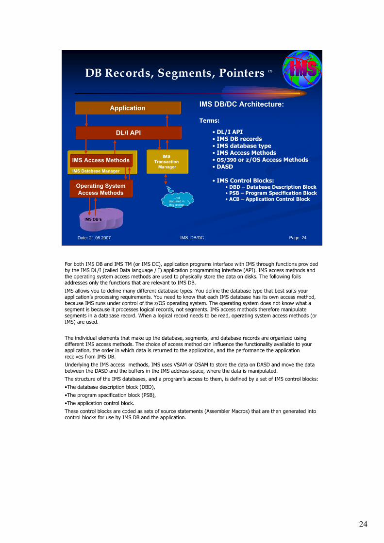
24
IMS_DB/DC Page: 24Date: 21.06.2007
DB Records, Segments, Pointers (2)
IMS Database Manager
Application
DL/I API
IMS Access Methods
Operating System
Access Methods
IMS
Transaction
Manager
IMS DB’s
…not discussed in this session
IMS DB/DC Architecture:
Terms:
• DL/I API• IMS DB records• IMS database type• IMS Access Methods• OS/390 or z/OS Access Methods • DASD
• IMS Control Blocks:• DBD – Database Description Block• PSB – Program Specification Block• ACB – Application Control Block
For both IMS DB and IMS TM (or IMS DC), application programs interface with IMS through functions provided by the IMS DL/I (called Data language / I) application programming interface (API). IMS access methods and the operating system access methods are used to physically store the data on disks. The following foils addresses only the functions that are relevant to IMS DB.
IMS allows you to define many different database types. You define the database type that best suits your application’s processing requirements. You need to know that each IMS database has its own access method, because IMS runs under control of the z/OS operating system. The operating system does not know what a segment is because it processes logical records, not segments. IMS access methods therefore manipulate segments in a database record. When a logical record needs to be read, operating system access methods (or IMS) are used.
The individual elements that make up the database, segments, and database records are organized using different IMS access methods. The choice of access method can influence the functionality available to your application, the order in which data is returned to the application, and the performance the application receives from IMS DB.
Underlying the IMS access methods, IMS uses VSAM or OSAM to store the data on DASD and move the data between the DASD and the buffers in the IMS address space, where the data is manipulated.
The structure of the IMS databases, and a program’s access to them, is defined by a set of IMS control blocks:
•The database description block (DBD),
•The program specification block (PSB),
•The application control block.
These control blocks are coded as sets of source statements (Assembler Macros) that are then generated into control blocks for use by IMS DB and the application.
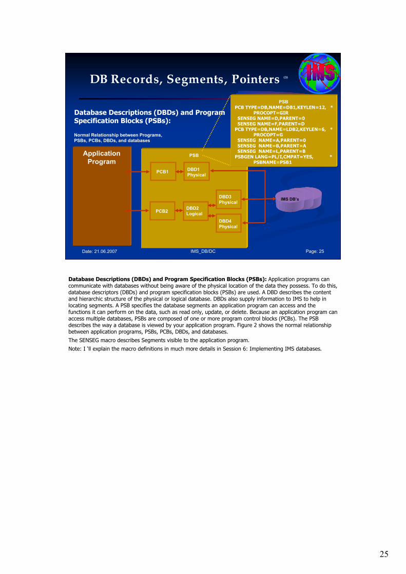
25
IMS_DB/DC Page: 25Date: 21.06.2007
DB Records, Segments, Pointers (3)
Database Descriptions (DBDs) and Program Specification Blocks (PSBs):
Application
Program
IMS DB’s
PSB
PCB1DBD1
Physical
DBD2
Logical
Normal Relationship between Programs,
PSBs, PCBs, DBDs, and databases
DBD3
Physical
DBD4
Physical
PCB2
PSB
PCB TYPE=DB,NAME=DB1,KEYLEN=12, *PROCOPT=GIR
SENSEG NAME=D,PARENT=0 SENSEG NAME=F,PARENT=D PCB TYPE=DB,NAME=LDB2,KEYLEN=6, *
PROCOPT=G SENSEG NAME=A,PARENT=0SENSEG NAME=B,PARENT=ASENSEG NAME=L,PARENT=BPSBGEN LANG=PL/I,CMPAT=YES, *
PSBNAME=PSB1
Database Descriptions (DBDs) and Program Specification Blocks (PSBs): Application programs can communicate with databases without being aware of the physical location of the data they possess. To do this, database descriptors (DBDs) and program specification blocks (PSBs) are used. A DBD describes the content and hierarchic structure of the physical or logical database. DBDs also supply information to IMS to help in locating segments. A PSB specifies the database segments an application program can access and the functions it can perform on the data, such as read only, update, or delete. Because an application program can access multiple databases, PSBs are composed of one or more program control blocks (PCBs). The PSB describes the way a database is viewed by your application program. Figure 2 shows the normal relationship between application programs, PSBs, PCBs, DBDs, and databases.
The SENSEG macro describes Segments visible to the application program.
Note: I ‘ll explain the macro definitions in much more details in Session 6: Implementing IMS databases.
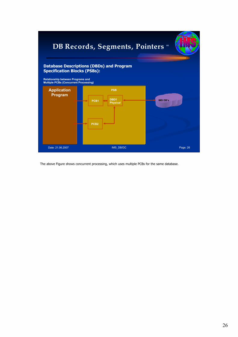
26
IMS_DB/DC Page: 26Date: 21.06.2007
DB Records, Segments, Pointers (4)
Database Descriptions (DBDs) and Program Specification Blocks (PSBs):
Application
Program
IMS DB’s
PSB
PCB1
PCB2
DBD1
Physical
Relationship between Programs and
Multiple PCBs (Concurrent Processing)
The above Figure shows concurrent processing, which uses multiple PCBs for the same database.
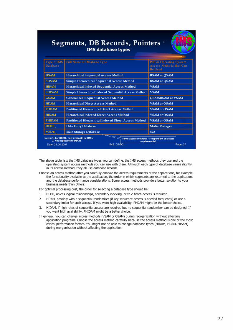
27
IMS_DB/DC Page: 27Date: 21.06.2007
Segments, DB Records, Pointers (5)
IMS database types
N/A Main Storage DatabaseMSDB 2
VSAM or OSAM Partitioned Hierarchical Indexed Direct Access MethodPHIDAM
VSAM or OSAMHierarchical Indexed Direct Access Method HIDAM
VSAM or OSAM Partitioned Hierarchical Direct Access Method PHDAM
VSAM or OSAM Hierarchical Direct Access MethodHDAM
QSAM/BSAM or VSAMGeneralized Sequential Access MethodGSAM
VSAM Simple Hierarchical Indexed Sequential Access Method SHISAM
VSAM Hierarchical Indexed Sequential Access Method HISAM
BSAM or QSAMSimple Hierarchical Sequential Access Method SHSAM
BSAM or QSAM Hierarchical Sequential Access MethodHSAM
Media Manager Data Entry Database DEDB 1
Full Name of Database Type Type of IMS Database
IMS or Operating System Access Methods that Can Be Used
Notes: 1. For DBCTL, only available to BMPs2. Not applicable to DBCTL
Term: Access methods -> dependent on access requirements!
The above table lists the IMS database types you can define, the IMS access methods they use and the operating system access methods you can use with them. Although each type of database varies slightly in its access method, they all use database records.
Choose an access method after you carefully analyze the access requirements of the applications, for example, the functionality available to the application, the order in which segments are returned to the application, and the database performance considerations. Some access methods provide a better solution to your business needs than others.
For optimal processing cost, the order for selecting a database type should be:
1. DEDB, unless logical relationships, secondary indexing, or true batch access is required.
2. HDAM, possibly with a sequential randomizer (if key sequence access is needed frequently) or use a secondary index for such access. If you want high availability, PHDAM might be the better choice.
3. HIDAM, if high rates of sequential access are required but no sequential randomizer can be designed. If you want high availability, PHIDAM might be a better choice.
In general, you can change access methods (VSAM or OSAM) during reorganization without affecting application programs. Choose the access method carefully because the access method is one of the most critical performance factors. You might not be able to change database types (HIDAM, HDAM, HISAM) during reorganization without affecting the application.
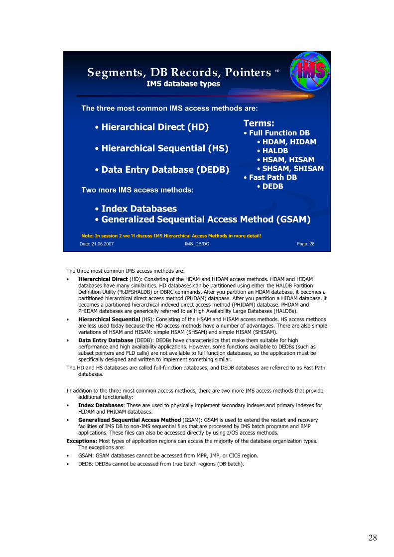
28
IMS_DB/DC Page: 28Date: 21.06.2007
Segments, DB Records, Pointers (6)
IMS database types
The three most common IMS access methods are:
• Hierarchical Direct (HD)
• Hierarchical Sequential (HS)
• Data Entry Database (DEDB)
Two more IMS access methods:
• Index Databases• Generalized Sequential Access Method (GSAM)
Terms:• Full Function DB
• HDAM, HIDAM• HALDB• HSAM, HISAM• SHSAM, SHISAM
• Fast Path DB• DEDB
Note: In session 2 we ‘ll discuss IMS Hierarchical Access Methods in more detail!
The three most common IMS access methods are:
• Hierarchical Direct (HD): Consisting of the HDAM and HIDAM access methods. HDAM and HIDAM databases have many similarities. HD databases can be partitioned using either the HALDB Partition Definition Utility (%DFSHALDB) or DBRC commands. After you partition an HDAM database, it becomes a partitioned hierarchical direct access method (PHDAM) database. After you partition a HIDAM database, it becomes a partitioned hierarchical indexed direct access method (PHIDAM) database. PHDAM and PHIDAM databases are generically referred to as High Availability Large Databases (HALDBs).
• Hierarchical Sequential (HS): Consisting of the HSAM and HISAM access methods. HS access methods are less used today because the HD access methods have a number of advantages. There are also simple variations of HSAM and HISAM: simple HSAM (SHSAM) and simple HISAM (SHISAM).
• Data Entry Database (DEDB): DEDBs have characteristics that make them suitable for high performance and high availability applications. However, some functions available to DEDBs (such as subset pointers and FLD calls) are not available to full function databases, so the application must be specifically designed and written to implement something similar.
The HD and HS databases are called full-function databases, and DEDB databases are referred to as Fast Path databases.
In addition to the three most common access methods, there are two more IMS access methods that provide additional functionality:
• Index Databases: These are used to physically implement secondary indexes and primary indexes for HIDAM and PHIDAM databases.
• Generalized Sequential Access Method (GSAM): GSAM is used to extend the restart and recovery facilities of IMS DB to non-IMS sequential files that are processed by IMS batch programs and BMP applications. These files can also be accessed directly by using z/OS access methods.
Exceptions: Most types of application regions can access the majority of the database organization types. The exceptions are:
• GSAM: GSAM databases cannot be accessed from MPR, JMP, or CICS region.
• DEDB: DEDBs cannot be accessed from true batch regions (DB batch).
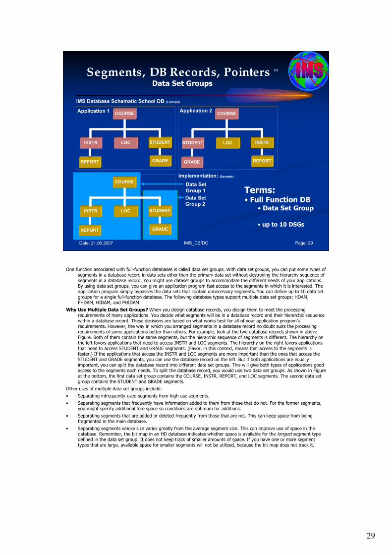
29
IMS_DB/DC Page: 29Date: 21.06.2007
Segments, DB Records, Pointers (7)
Data Set Groups
Terms:• Full Function DB
• Data Set Group
• up to 10 DSGs
IMS Database Schematic School DB (Example)
COURSE
INSTR LOC STUDENT
REPORT GRADE
Application 1COURSE
STUDENT LOC INSTR
GRADE REPORT
Application 2
COURSE
INSTR LOC STUDENT
REPORT GRADE
Data Set
Group 1
Data Set
Group 2
Implementation: (Example)
One function associated with full-function databases is called data set groups. With data set groups, you can put some types of segments in a database record in data sets other than the primary data set without destroying the hierarchy sequence of segments in a database record. You might use dataset groups to accommodate the different needs of your applications. By using data set groups, you can give an application program fast access to the segments in which it is interested. The application program simply bypasses the data sets that contain unnecessary segments. You can define up to 10 data set groups for a single full-function database. The following database types support multiple data set groups: HDAM, PHDAM, HIDAM, and PHIDAM.
Why Use Multiple Data Set Groups? When you design database records, you design them to meet the processing requirements of many applications. You decide what segments will be in a database record and their hierarchic sequence within a database record. These decisions are based on what works best for all of your application program’s requirements. However, the way in which you arranged segments in a database record no doubt suits the processing requirements of some applications better than others. For example, look at the two database records shown in above Figure. Both of them contain the same segments, but the hierarchic sequence of segments is different. The hierarchy on the left favors applications that need to access INSTR and LOC segments. The hierarchy on the right favors applications that need to access STUDENT and GRADE segments. (Favor, in this context, means that access to the segments is faster.) If the applications that access the INSTR and LOC segments are more important than the ones that access the STUDENT and GRADE segments, you can use the database record on the left. But if both applications are equally important, you can split the database record into different data set groups. This will give both types of applications good access to the segments each needs. To split the database record, you would use two data set groups. As shown in Figure at the bottom, the first data set group contains the COURSE, INSTR, REPORT, and LOC segments. The second data set group contains the STUDENT and GRADE segments.
Other uses of multiple data set groups include:
• Separating infrequently-used segments from high-use segments.
• Separating segments that frequently have information added to them from those that do not. For the former segments, you might specify additional free space so conditions are optimum for additions.
• Separating segments that are added or deleted frequently from those that are not. This can keep space from being fragmented in the main database.
• Separating segments whose size varies greatly from the average segment size. This can improve use of space in the database. Remember, the bit map in an HD database indicates whether space is available for the longest segment type defined in the data set group. It does not keep track of smaller amounts of space. If you have one or more segment types that are large, available space for smaller segments will not be utilized, because the bit map does not track it.
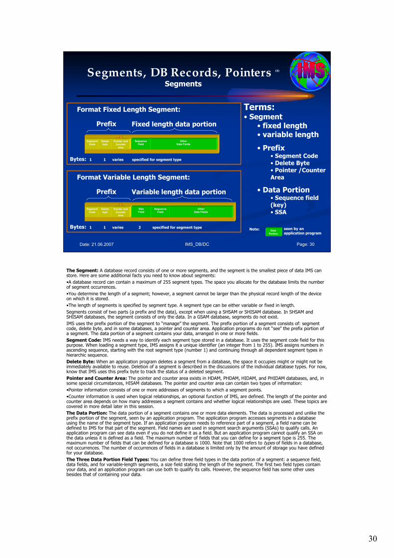
30
IMS_DB/DC Page: 30Date: 21.06.2007
Segments, DB Records, Pointers (8)
Segments
Segment
Code
Delete
byte
Pointer and
Counter
area
Prefix Variable length data portion
Format Variable Length Segment:
Bytes: 1 1 varies 2 specified for segment type
Size
FieldSequence
Field
Other
Data Fields
Segment
Code
Delete
byte
Pointer and
Counter
area
Sequence
Field
Other
Data Fields
Prefix Fixed length data portion
Format Fixed Length Segment:
Bytes: 1 1 varies specified for segment type
Terms:• Segment
• fixed length• variable length
• Prefix• Segment Code• Delete Byte• Pointer /Counter Area
• Data Portion• Sequence field (key)• SSA
Data
Portion
seen by anapplication program
Note:
The Segment: A database record consists of one or more segments, and the segment is the smallest piece of data IMS can store. Here are some additional facts you need to know about segments:
•A database record can contain a maximum of 255 segment types. The space you allocate for the database limits the number of segment occurrences.
•You determine the length of a segment; however, a segment cannot be larger than the physical record length of the device on which it is stored.
•The length of segments is specified by segment type. A segment type can be either variable or fixed in length.
Segments consist of two parts (a prefix and the data), except when using a SHSAM or SHISAM database. In SHSAM and SHISAM databases, the segment consists of only the data. In a GSAM database, segments do not exist.
IMS uses the prefix portion of the segment to “manage” the segment. The prefix portion of a segment consists of: segment code, delete byte, and in some databases, a pointer and counter area. Application programs do not “see” the prefix portion of a segment. The data portion of a segment contains your data, arranged in one or more fields.
Segment Code: IMS needs a way to identify each segment type stored in a database. It uses the segment code field for this purpose. When loading a segment type, IMS assigns it a unique identifier (an integer from 1 to 255). IMS assigns numbers in ascending sequence, starting with the root segment type (number 1) and continuing through all dependent segment types in hierarchic sequence.
Delete Byte: When an application program deletes a segment from a database, the space it occupies might or might not be immediately available to reuse. Deletion of a segment is described in the discussions of the individual database types. For now,know that IMS uses this prefix byte to track the status of a deleted segment.
Pointer and Counter Area: The pointer and counter area exists in HDAM, PHDAM, HIDAM, and PHIDAM databases, and, in some special circumstances, HISAM databases. The pointer and counter area can contain two types of information:
•Pointer information consists of one or more addresses of segments to which a segment points.
•Counter information is used when logical relationships, an optional function of IMS, are defined. The length of the pointer and counter area depends on how many addresses a segment contains and whether logical relationships are used. These topics are covered in more detail later in this session.
The Data Portion: The data portion of a segment contains one or more data elements. The data is processed and unlike the prefix portion of the segment, seen by an application program. The application program accesses segments in a database using the name of the segment type. If an application program needs to reference part of a segment, a field name can be defined to IMS for that part of the segment. Field names are used in segment search arguments (SSAs) to qualify calls. An application program can see data even if you do not define it as a field. But an application program cannot qualify an SSA on the data unless it is defined as a field. The maximum number of fields that you can define for a segment type is 255. The maximum number of fields that can be defined for a database is 1000. Note that 1000 refers to types of fields in a database, not occurrences. The number of occurrences of fields in a database is limited only by the amount of storage you have defined for your database.
The Three Data Portion Field Types: You can define three field types in the data portion of a segment: a sequence field, data fields, and for variable-length segments, a size field stating the length of the segment. The first two field types contain your data, and an application program can use both to qualify its calls. However, the sequence field has some other uses besides that of containing your data.
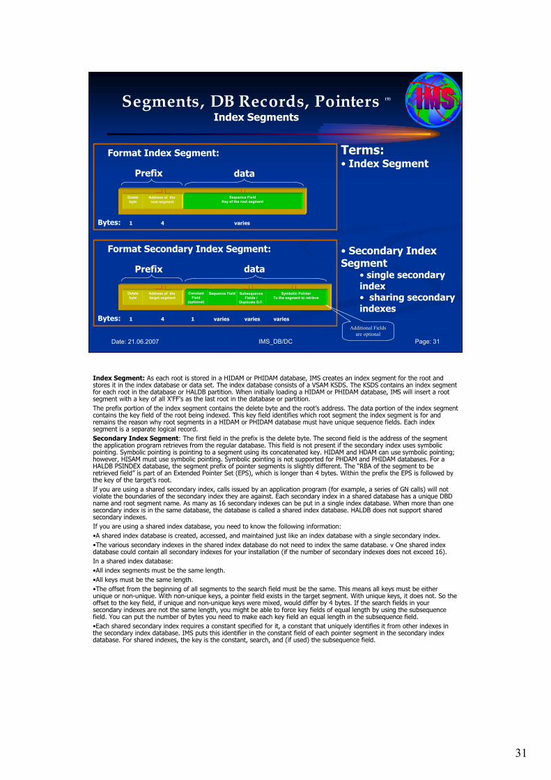
31
IMS_DB/DC Page: 31Date: 21.06.2007
Segments, DB Records, Pointers (9)
Index Segments
Terms:• Index Segment
• Secondary Index Segment
• single secondary index• sharing secondary indexes
Delete
byte
Address of the
root segment
Sequence Field
Key of the root segment
Prefix data
Format Index Segment:
Bytes: 1 4 varies
Delete
byte
Address of the
target segment
Prefix data
Format Secondary Index Segment:
Bytes: 1 4 1 varies varies varies
Constant
Field
(optional)
Sequence Field Subsequence
Fields /
Duplicate D.F.
Symbolic Pointer
To the segment to retrieve
Additional Fields
are optional
Index Segment: As each root is stored in a HIDAM or PHIDAM database, IMS creates an index segment for the root and stores it in the index database or data set. The index database consists of a VSAM KSDS. The KSDS contains an index segment for each root in the database or HALDB partition. When initially loading a HIDAM or PHIDAM database, IMS will insert a root segment with a key of all X'FF's as the last root in the database or partition.
The prefix portion of the index segment contains the delete byte and the root’s address. The data portion of the index segment contains the key field of the root being indexed. This key field identifies which root segment the index segment is for and remains the reason why root segments in a HIDAM or PHIDAM database must have unique sequence fields. Each index segment is a separate logical record.
Secondary Index Segment: The first field in the prefix is the delete byte. The second field is the address of the segment the application program retrieves from the regular database. This field is not present if the secondary index uses symbolic pointing. Symbolic pointing is pointing to a segment using its concatenated key. HIDAM and HDAM can use symbolic pointing; however, HISAM must use symbolic pointing. Symbolic pointing is not supported for PHDAM and PHIDAM databases. For a HALDB PSINDEX database, the segment prefix of pointer segments is slightly different. The “RBA of the segment to be retrieved field” is part of an Extended Pointer Set (EPS), which is longer than 4 bytes. Within the prefix the EPS is followed by the key of the target’s root.
If you are using a shared secondary index, calls issued by an application program (for example, a series of GN calls) will not violate the boundaries of the secondary index they are against. Each secondary index in a shared database has a unique DBD name and root segment name. As many as 16 secondary indexes can be put in a single index database. When more than one secondary index is in the same database, the database is called a shared index database. HALDB does not support shared secondary indexes.
If you are using a shared index database, you need to know the following information:
•A shared index database is created, accessed, and maintained just like an index database with a single secondary index.
•The various secondary indexes in the shared index database do not need to index the same database. v One shared index database could contain all secondary indexes for your installation (if the number of secondary indexes does not exceed 16).
In a shared index database:
•All index segments must be the same length.
•All keys must be the same length.
•The offset from the beginning of all segments to the search field must be the same. This means all keys must be either unique or non-unique. With non-unique keys, a pointer field exists in the target segment. With unique keys, it does not. So the offset to the key field, if unique and non-unique keys were mixed, would differ by 4 bytes. If the search fields in your secondary indexes are not the same length, you might be able to force key fields of equal length by using the subsequence field. You can put the number of bytes you need to make each key field an equal length in the subsequence field.
•Each shared secondary index requires a constant specified for it, a constant that uniquely identifies it from other indexes in the secondary index database. IMS puts this identifier in the constant field of each pointer segment in the secondary index database. For shared indexes, the key is the constant, search, and (if used) the subsequence field.
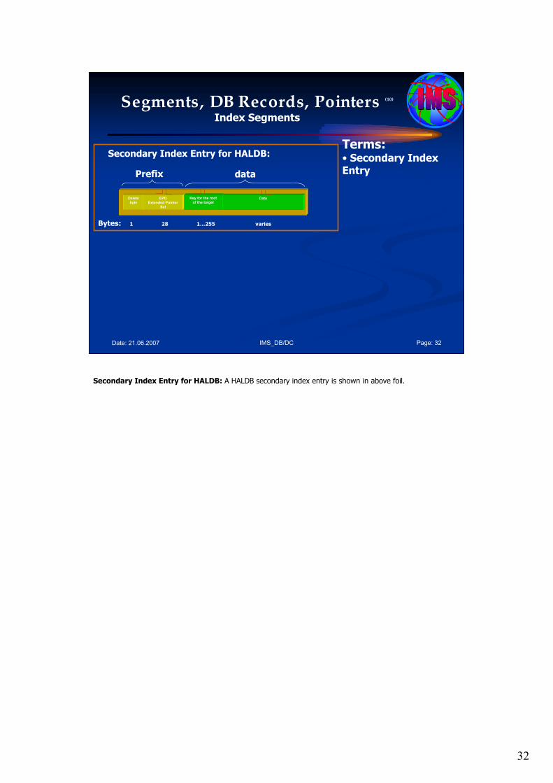
32
IMS_DB/DC Page: 32Date: 21.06.2007
Segments, DB Records, Pointers (10)
Index Segments
Terms:• Secondary Index Entry
Delete
byte
EPD
Extended Pointer
Set
Key for the root
of the target
Prefix data
Secondary Index Entry for HALDB:
Bytes: 1 28 1…255 varies
Data
Secondary Index Entry for HALDB: A HALDB secondary index entry is shown in above foil.

33
IMS_DB/DC Page: 33Date: 21.06.2007
Segments, DB Records, Pointers (11)
HD Pointers
Terms:
Types of Pointers:
• Physical child pointers, • Physical twin pointers,
• Hierarchic pointers.
Pointer:First, LastForward, Backward
Forward, Backward
… mixed pointers
Before looking in detail at how HD databases are stored and processed, you need to become familiar with: The various types of pointers you can specify for a HD database.
Types of Pointers You Can Specify: The hierarchic sequence of segments in a database record using the sequential access methods is maintained by keeping segments physically adjacent to each other in storage. In the HD access methods, segments in a database record are kept in hierarchic sequence using direct-address pointers. Except for a few special cases, each prefix in an HD segment contains one or more pointers. Each pointer is 4 bytes long and consists of the relative byte address of the segment to which it points. Relative, in this case, means relative to the beginning of the data set. Several different types of direct-address pointers exist, and you will see how each works in the topics that follow in this session. However, there are three basic types:
•Hierarchic pointers, which point from one segment to the next in either forward or forward and backward hierarchic sequence,
•Physical child pointers, which point from a parent to each of its first or first and last children, for each child segment type,
•Physical twin pointers, which point forward or forward and backward from one segment occurrence of a segment type to the next, under the same parent.
When segments in a database record are typically processed in hierarchic sequence, use hierarchic pointers. When segments in a database record are typically processed randomly, use a combination of physical child and physical twin pointers. One thing to keep in mind while reading about pointers is that the different types, subject to some rules, can be mixed within a database record. However, because pointers are specified by segment type, all occurrences of the same segment type have the same type of pointer. Additional we have to look at different type of pointers; for physical child pointers we have physical child first and optional physical child last pointers, for the other types we have forward and optional backward pointers.
Additional we have to discuss, how pointers can be mixed.

34
IMS_DB/DC Page: 34Date: 21.06.2007
Segments, DB Records, Pointers (12)
Database Segments andPointers
Terms:Prefix:
Pointer -> RBA• PTF – Physical Twin Forward• PTB – Physical Twin Backward• PCF – Physical Child First• PCL – Physical Child Last
A first look at Pointers…
… PTF PTB PCF PCF Root 1
… PTF Dependent 1
Occurrence 1
… PTF PTB PCF PCF Root 2
… PTF Dependent 2
Occurrence 1
… PTF Dependent 1
Occurrence 2
… PTF Dependent 1
Occurrence 1
… PTF Dependent 2
Occurrence 1
… PTF Dependent 2
Occurrence 2
… PTF Dependent 2
Occurrence 3
Next Root Segment
As shown before, in addition to the application data, each segment contains control information that is used by IMS. The control information is placed at the beginning of the segment in a segment prefix. The prefix is automatically maintained by IMS and is not accessible to the application. The control information in the prefix consists of various flags, descriptive fields (segment type code and delete byte), and pointers to implement the hierarchical structure and access paths. The contents of the prefix will vary - as shown in the next foil -, depending on the IMS access method and options chosen when the database is defined.
The RBA pointers in above figure consist of the relative offset (number of bytes) of the segment being pointed at, from the start of the data set being used to store the data. This is the relative byte address (RBA). For example, a root segment would contain pointer fields in the prefix for, at a minimum, all of the dependent segment types under the root. IMS will automatically define the minimum set of pointers to maintain the hierarchical structure. The database designer can also specify additional predefined types of pointers, in addition to those necessary for the minimum hierarchical structure. This pointer selection can influence the performance of applications using the database.
The above figure shows database segments with their pointers: physical twin forward (PTF), physical twin backward (PTB), and physical child first (PCF).
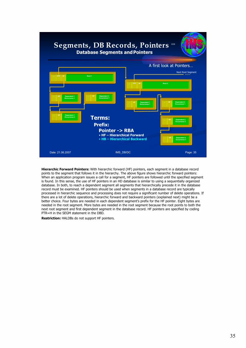
35
IMS_DB/DC Page: 35Date: 21.06.2007
Segments, DB Records, Pointers (13)
Database Segments andPointers
Terms:Prefix:
Pointer -> RBA• HF – Hierarchical Forward• HB – Hierarchical Backward
A first look at Pointers…
… PTF HF Root 1
… HF Dependent 1
Occurrence 1
… PTF HF Root 2
… HF Dependent 2
Occurrence 1
… HF Dependent 1
Occurrence 2
… HF Dependent 1
Occurrence 1
… HF Dependent 2
Occurrence 1
… HF Dependent 2
Occurrence 2
… HF Dependent 2
Occurrence 3
Next Root Segment
Hierarchic Forward Pointers: With hierarchic forward (HF) pointers, each segment in a database record points to the segment that follows it in the hierarchy. The above figure shows hierarchic forward pointers: When an application program issues a call for a segment, HF pointers are followed until the specified segment is found. In this sense, the use of HF pointers in an HD database is similar to using a sequentially organized database. In both, to reach a dependent segment all segments that hierarchically precede it in the database record must be examined. HF pointers should be used when segments in a database record are typically processed in hierarchic sequence and processing does not require a significant number of delete operations. If there are a lot of delete operations, hierarchic forward and backward pointers (explained next) might be a better choice. Four bytes are needed in each dependent segment’s prefix for the HF pointer. Eight bytes are needed in the root segment. More bytes are needed in the root segment because the root points to both the next root segment and first dependent segment in the database record. HF pointers are specified by coding PTR=H in the SEGM statement in the DBD.
Restriction: HALDBs do not support HF pointers.
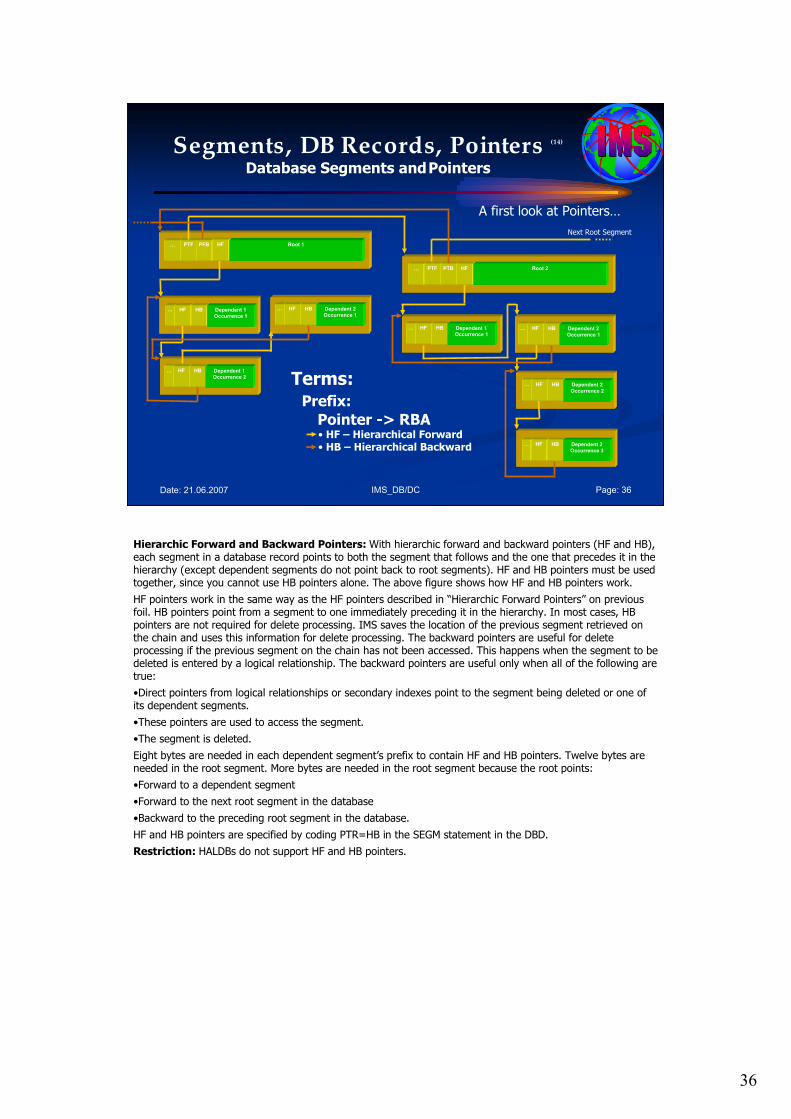
36
IMS_DB/DC Page: 36Date: 21.06.2007
Segments, DB Records, Pointers (14)
Database Segments andPointers
A first look at Pointers…
Terms:Prefix:
Pointer -> RBA• HF – Hierarchical Forward• HB – Hierarchical Backward
… PTF PFB
…
… PTF
Next Root Segment
HF
HF HB Dependent 1
Occurrence 1
… HF HB Dependent 1
Occurrence 2
Root 1
… HF HB Dependent 2
Occurrence 1
PTB HF Root 2
… HF HB Dependent 1
Occurrence 1
… HF HB Dependent 2
Occurrence 1
… HF HB Dependent 2
Occurrence 2
… HF HB Dependent 2
Occurrence 3
Hierarchic Forward and Backward Pointers: With hierarchic forward and backward pointers (HF and HB), each segment in a database record points to both the segment that follows and the one that precedes it in the hierarchy (except dependent segments do not point back to root segments). HF and HB pointers must be used together, since you cannot use HB pointers alone. The above figure shows how HF and HB pointers work.
HF pointers work in the same way as the HF pointers described in “Hierarchic Forward Pointers” on previous foil. HB pointers point from a segment to one immediately preceding it in the hierarchy. In most cases, HB pointers are not required for delete processing. IMS saves the location of the previous segment retrieved on the chain and uses this information for delete processing. The backward pointers are useful for delete processing if the previous segment on the chain has not been accessed. This happens when the segment to be deleted is entered by a logical relationship. The backward pointers are useful only when all of the following are true:
•Direct pointers from logical relationships or secondary indexes point to the segment being deleted or one of its dependent segments.
•These pointers are used to access the segment.
•The segment is deleted.
Eight bytes are needed in each dependent segment’s prefix to contain HF and HB pointers. Twelve bytes are needed in the root segment. More bytes are needed in the root segment because the root points:
•Forward to a dependent segment
•Forward to the next root segment in the database
•Backward to the preceding root segment in the database.
HF and HB pointers are specified by coding PTR=HB in the SEGM statement in the DBD.
Restriction: HALDBs do not support HF and HB pointers.
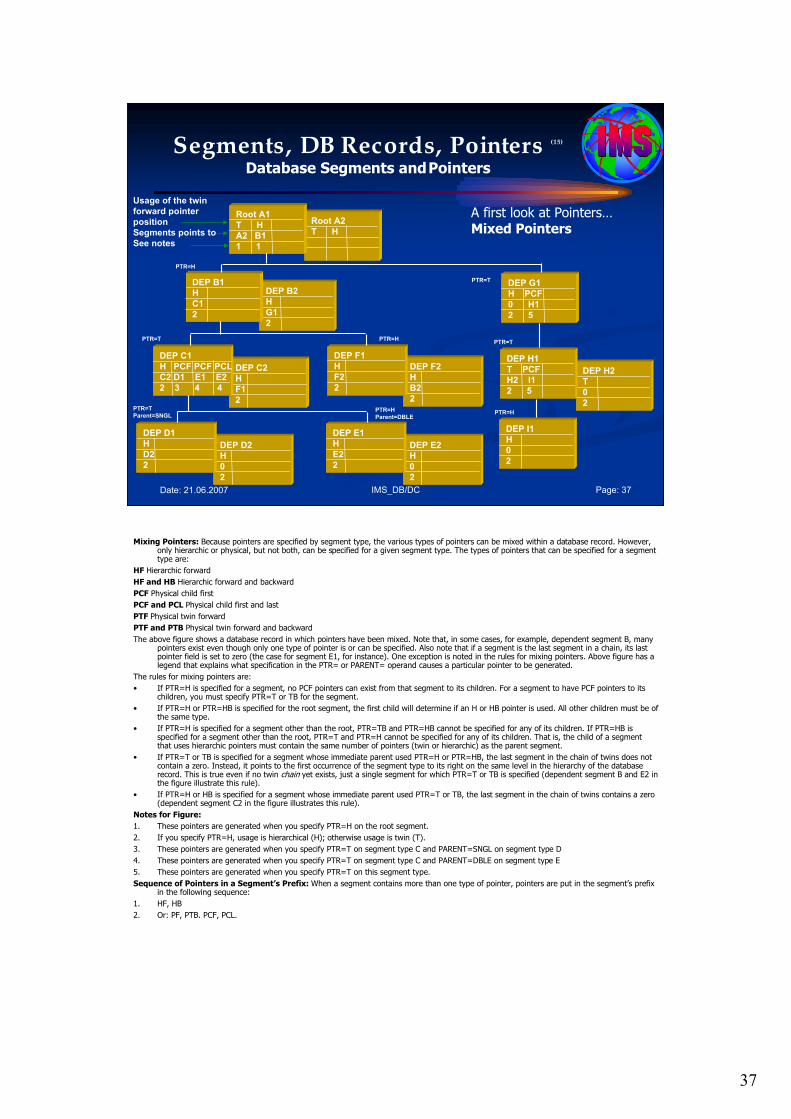
37
IMS_DB/DC Page: 37Date: 21.06.2007
Segments, DB Records, Pointers (15)
Database Segments andPointers
A first look at Pointers…Mixed Pointers
DEP H2
T
0
2
DEP F2
H
B2
2
DEP D2
H
0
2
DEP C2
H
F1
2
Root A2
T H
DEP B2
H
G1
2
Root A1
T H
A2 B1
1 1
DEP B1
H
C1
2
DEP C1
H PCF PCF PCL
C2 D1 E1 E2
2 3 4 4
DEP D1
H
D2
2
DEP F1
H
F2
2
DEP G1
H PCF
0 H1
2 5
DEP H1
T PCF
H2 I1
2 5
DEP I1
H
0
2
DEP E2
H
0
2
DEP E1
H
E2
2
Usage of the twin
forward pointer
position
Segments points to
See notes
PTR=H
PTR=T
PTR=T
Parent=SNGL
PTR=H
PTR=H
Parent=DBLE
PTR=T
PTR=T
PTR=H
Mixing Pointers: Because pointers are specified by segment type, the various types of pointers can be mixed within a database record. However, only hierarchic or physical, but not both, can be specified for a given segment type. The types of pointers that can be specified for a segment type are:
HF Hierarchic forward
HF and HB Hierarchic forward and backward
PCF Physical child first
PCF and PCL Physical child first and last
PTF Physical twin forward
PTF and PTB Physical twin forward and backward
The above figure shows a database record in which pointers have been mixed. Note that, in some cases, for example, dependent segment B, many pointers exist even though only one type of pointer is or can be specified. Also note that if a segment is the last segment in a chain, its last pointer field is set to zero (the case for segment E1, for instance). One exception is noted in the rules for mixing pointers. Above figure has a legend that explains what specification in the PTR= or PARENT= operand causes a particular pointer to be generated.
The rules for mixing pointers are:
• If PTR=H is specified for a segment, no PCF pointers can exist from that segment to its children. For a segment to have PCF pointers to its children, you must specify PTR=T or TB for the segment.
• If PTR=H or PTR=HB is specified for the root segment, the first child will determine if an H or HB pointer is used. All other children must be of the same type.
• If PTR=H is specified for a segment other than the root, PTR=TB and PTR=HB cannot be specified for any of its children. If PTR=HB is specified for a segment other than the root, PTR=T and PTR=H cannot be specified for any of its children. That is, the child of a segment that uses hierarchic pointers must contain the same number of pointers (twin or hierarchic) as the parent segment.
• If PTR=T or TB is specified for a segment whose immediate parent used PTR=H or PTR=HB, the last segment in the chain of twins does not contain a zero. Instead, it points to the first occurrence of the segment type to its right on the same level in the hierarchy of the database record. This is true even if no twin chain yet exists, just a single segment for which PTR=T or TB is specified (dependent segment B and E2 in the figure illustrate this rule).
• If PTR=H or HB is specified for a segment whose immediate parent used PTR=T or TB, the last segment in the chain of twins contains a zero (dependent segment C2 in the figure illustrates this rule).
Notes for Figure:
1. These pointers are generated when you specify PTR=H on the root segment.
2. If you specify PTR=H, usage is hierarchical (H); otherwise usage is twin (T).
3. These pointers are generated when you specify PTR=T on segment type C and PARENT=SNGL on segment type D
4. These pointers are generated when you specify PTR=T on segment type C and PARENT=DBLE on segment type E
5. These pointers are generated when you specify PTR=T on this segment type.
Sequence of Pointers in a Segment’s Prefix: When a segment contains more than one type of pointer, pointers are put in the segment’s prefix in the following sequence:
1. HF, HB
2. Or: PF, PTB. PCF, PCL.
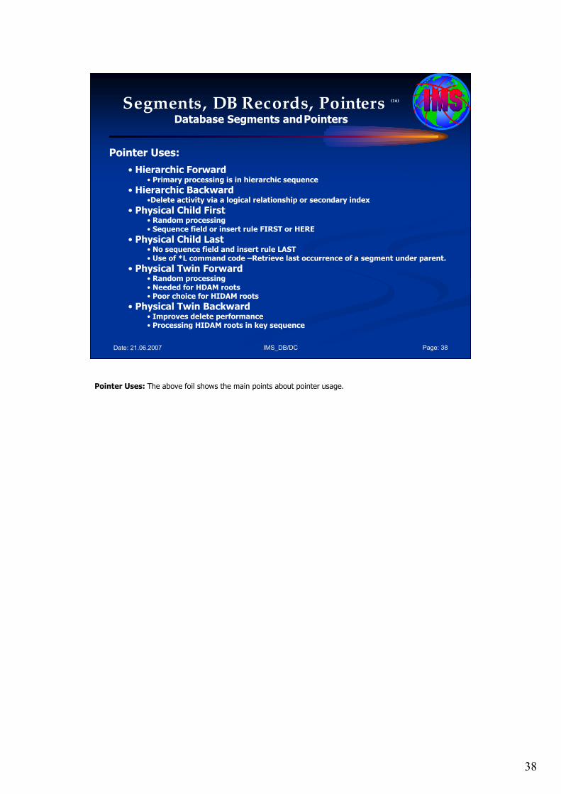
38
IMS_DB/DC Page: 38Date: 21.06.2007
Segments, DB Records, Pointers (16)
Database Segments andPointers
Pointer Uses:
• Hierarchic Forward• Primary processing is in hierarchic sequence
• Hierarchic Backward•Delete activity via a logical relationship or secondary index
• Physical Child First• Random processing• Sequence field or insert rule FIRST or HERE
• Physical Child Last• No sequence field and insert rule LAST• Use of *L command code –Retrieve last occurrence of a segment under parent.
• Physical Twin Forward• Random processing• Needed for HDAM roots• Poor choice for HIDAM roots
• Physical Twin Backward• Improves delete performance• Processing HIDAM roots in key sequence
Pointer Uses: The above foil shows the main points about pointer usage.
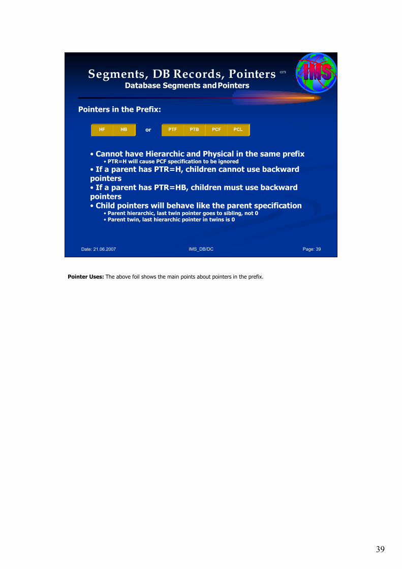
39
IMS_DB/DC Page: 39Date: 21.06.2007
Segments, DB Records, Pointers (17)
Database Segments andPointers
Pointers in the Prefix:
• Cannot have Hierarchic and Physical in the same prefix• PTR=H will cause PCF specification to be ignored
• If a parent has PTR=H, children cannot use backward pointers• If a parent has PTR=HB, children must use backward pointers• Child pointers will behave like the parent specification
• Parent hierarchic, last twin pointer goes to sibling, not 0• Parent twin, last hierarchic pointer in twins is 0
HF HB PTF PTB PCF PCLor
Pointer Uses: The above foil shows the main points about pointers in the prefix.
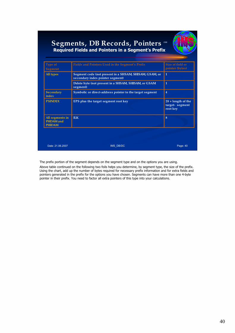
40
IMS_DB/DC Page: 40Date: 21.06.2007
Segments, DB Records, Pointers (18)
Required Fields and Pointers in a Segment’s Prefix
8ILKAll segments in PHDAM and PHIDAM
28 + length of the target- segment root key
EPS plus the target segment root key PSINDEX
4Symbolic or direct-address pointer to the target segmentSecondary index
1Delete byte (not present in a SHSAM, SHISAM, or GSAM segment)
1 Segment code (not present in a SHSAM, SHISAM, GSAM, or secondary index pointer segment)
All types
Fields and Pointers Used in the Segment’s PrefixType of
Segment
Size of field or pointer (bytes)
The prefix portion of the segment depends on the segment type and on the options you are using.
Above table continued on the following two foils helps you determine, by segment type, the size of the prefix. Using the chart, add up the number of bytes required for necessary prefix information and for extra fields and pointers generated in the prefix for the options you have chosen. Segments can have more than one 4-byte pointer in their prefix. You need to factor all extra pointers of this type into your calculations.
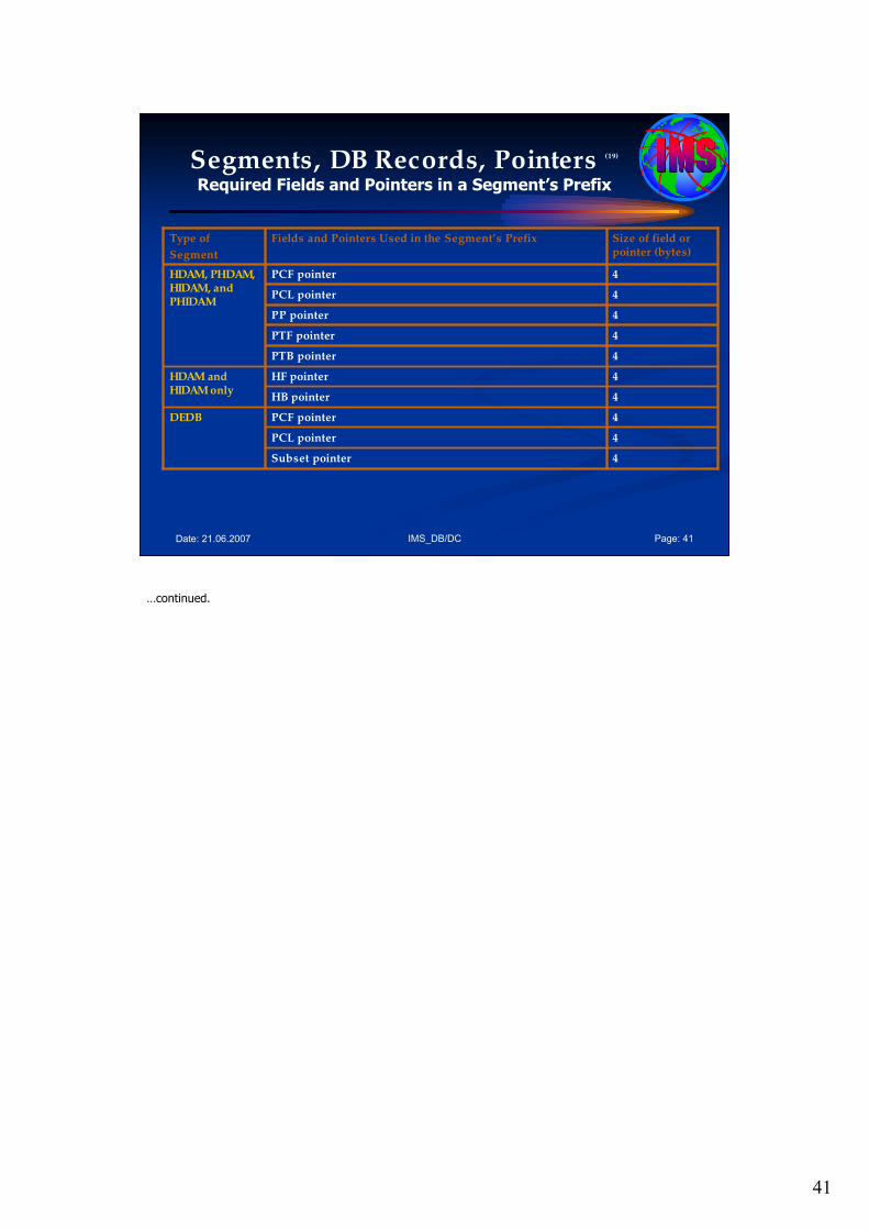
41
IMS_DB/DC Page: 41Date: 21.06.2007
Segments, DB Records, Pointers (19)
Required Fields and Pointers in a Segment’s Prefix
4Subset pointer
4PCL pointer
4HB pointer
4PTB pointer
4PTF pointer
4PP pointer
4PCL pointer
4PCF pointerDEDB
4HF pointerHDAM and HIDAM only
4PCF pointerHDAM, PHDAM, HIDAM, and PHIDAM
Fields and Pointers Used in the Segment’s PrefixType of
Segment
Size of field or pointer (bytes)
…continued.
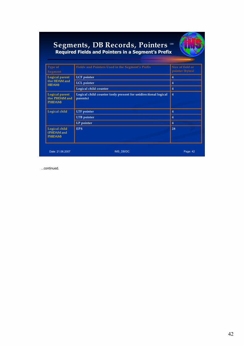
42
IMS_DB/DC Page: 42Date: 21.06.2007
Segments, DB Records, Pointers (20)
Required Fields and Pointers in a Segment’s Prefix
4LP pointer
4LTF pointerLogical child
28EPS
4LTB pointer
4Logical child counter
4LCL pointer
Logical child (PHDAM and PHIDAM)
4Logical child counter (only present for unidirectional logical parents)
Logical parent (for PHDAM and PHIDAM)
4LCF pointerLogical parent (for HDAM and HIDAM)
Fields and Pointers Used in the Segment’s PrefixType of
Segment
Size of field or pointer (bytes)
…continued.
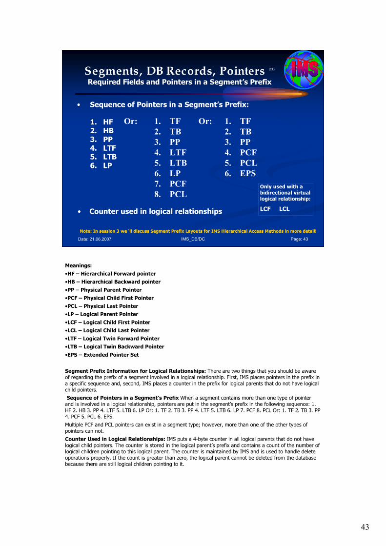
43
IMS_DB/DC Page: 43Date: 21.06.2007
Segments, DB Records, Pointers (21)
Required Fields and Pointers in a Segment’s Prefix
• Sequence of Pointers in a Segment’s Prefix:
1. HF 2. HB 3. PP 4. LTF 5. LTB 6. LP
1. TF
2. TB
3. PP
4. LTF
5. LTB
6. LP
7. PCF
8. PCL
Or: 1. TF
2. TB
3. PP
4. PCF
5. PCL
6. EPS
Or:
• Counter used in logical relationships
Note: In session 3 we ‘ll discuss Segment Prefix Layouts for IMS Hierarchical Access Methods in more detail!
Only used with a bidirectional virtual logical relationship:
LCF LCL
Meanings:
•HF – Hierarchical Forward pointer
•HB – Hierarchical Backward pointer
•PP – Physical Parent Pointer
•PCF – Physical Child First Pointer
•PCL – Physical Last Pointer
•LP – Logical Parent Pointer
•LCF – Logical Child First Pointer
•LCL – Logical Child Last Pointer
•LTF – Logical Twin Forward Pointer
•LTB – Logical Twin Backward Pointer
•EPS – Extended Pointer Set
Segment Prefix Information for Logical Relationships: There are two things that you should be aware of regarding the prefix of a segment involved in a logical relationship. First, IMS places pointers in the prefix in a specific sequence and, second, IMS places a counter in the prefix for logical parents that do not have logical child pointers.
Sequence of Pointers in a Segment’s Prefix When a segment contains more than one type of pointer and is involved in a logical relationship, pointers are put in the segment’s prefix in the following sequence: 1. HF 2. HB 3. PP 4. LTF 5. LTB 6. LP Or: 1. TF 2. TB 3. PP 4. LTF 5. LTB 6. LP 7. PCF 8. PCL Or: 1. TF 2. TB 3. PP 4. PCF 5. PCL 6. EPS.
Multiple PCF and PCL pointers can exist in a segment type; however, more than one of the other types of pointers can not.
Counter Used in Logical Relationships: IMS puts a 4-byte counter in all logical parents that do not have logical child pointers. The counter is stored in the logical parent’s prefix and contains a count of the number of logical children pointing to this logical parent. The counter is maintained by IMS and is used to handle delete operations properly. If the count is greater than zero, the logical parent cannot be deleted from the database because there are still logical children pointing to it.
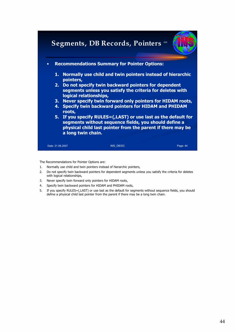
44
IMS_DB/DC Page: 44Date: 21.06.2007
Segments, DB Records, Pointers (22)
• Recommendations Summary for Pointer Options:
1. Normally use child and twin pointers instead of hierarchic pointers,
2. Do not specify twin backward pointers for dependent segments unless you satisfy the criteria for deletes with logical relationships,
3. Never specify twin forward only pointers for HIDAM roots,4. Specify twin backward pointers for HIDAM and PHIDAM
roots,5. If you specify RULES=(,LAST) or use last as the default for
segments without sequence fields, you should define a physical child last pointer from the parent if there may be a long twin chain.
The Recommendations for Pointer Options are:
1. Normally use child and twin pointers instead of hierarchic pointers,
2. Do not specify twin backward pointers for dependent segments unless you satisfy the criteria for deletes with logical relationships,
3. Never specify twin forward only pointers for HIDAM roots,
4. Specify twin backward pointers for HIDAM and PHIDAM roots,
5. If you specify RULES=(,LAST) or use last as the default for segments without sequence fields, you should define a physical child last pointer from the parent if there may be a long twin chain.
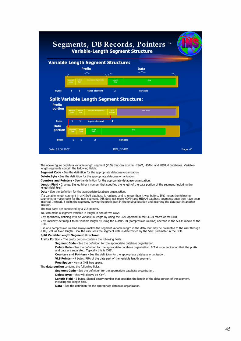
45
IMS_DB/DC Page: 45Date: 21.06.2007
Segments, DB Records, Pointers (23)
Variable-Length Segment Structure
Variable Length Segment Structure:
segment
code
delete
byte
counters and pointers Length
fielddata
Prefix Data
Bytes 1 1 4 per element 2 variable
Split Variable Length Segment Structure:
segment
code
delete
byte
counters and pointers Free space
Prefixportion
Bytes 1 1 4 per element 4
VLS
pointer
segment
code
delete
byteLength
fielddata
Bytes 1 1 2 variable
Dataportion
The above figure depicts a variable-length segment (VLS) that can exist in HISAM, HDAM, and HIDAM databases. Variable-length segments contain the following fields:
Segment Code - See the definition for the appropriate database organization.
Delete Byte - See the definition for the appropriate database organization.
Counters and Pointers - See the definition for the appropriate database organization.
Length Field - 2 bytes. Signed binary number that specifies the length of the data portion of the segment, including the length field itself.
Data - See the definition for the appropriate database organization.
If a variable-length segment in a HISAM database is replaced and is longer than it was before, IMS moves the following segments to make room for the new segment. IMS does not move HDAM and HIDAM database segments once they have been inserted. Instead, it splits the segment, leaving the prefix part in the original location and inserting the data part in another location.
The two parts are connected by a VLS pointer.
You can make a segment variable in length in one of two ways:
• by specifically defining it to be variable in length by using the SIZE operand in the SEGM macro of the DBD
• by implicitly defining it to be variable length by using the COMPRTN (compression routine) operand in the SEGM macro of the DBD.
Use of a compression routine always makes the segment variable length in the data, but may be presented to the user through a DL/I call as fixed length. How the user sees the segment data is determined by the SIZE parameter in the DBD.
Split Variable Length Segment Structure:
Prefix Portion - The prefix portion contains the following fields:
Segment Code - See the definition for the appropriate database organization.
Delete Byte - See the definition for the appropriate database organization. BIT 4 is on, indicating that the prefix and data are separated. Typically this is X'08'.
Counters and Pointers - See the definition for the appropriate database organization.
VLS Pointer - 4 bytes. RBA of the data part of the variable length segment.
Free Space - Normal IMS free space.
The data portion contains the following fields:
Segment Code - See the definition for the appropriate database organization.
Delete Byte - This will always be X'FF'.
Length Field - 2 bytes. Signed binary number that specifies the length of the data portion of the segment, including the length field.
Data - See the definition for the appropriate database organization.
46
IMS_DB/DC Page: 46Date: 21.06.2007
Agenda Session 2: Database Basics
1. Basic Terms
2. Physical Database
3. Logical Database / Relationships
4. Secondary Indexes
5. How data is stored/retrieved in a DB
6. DB Records, Segments, Pointers
7. Database Segments & Data Area
8. Points not addressed
7. Database Segments & Data Area
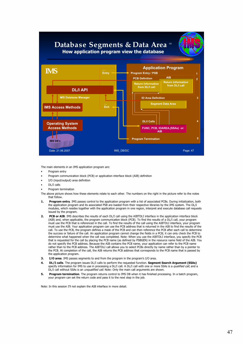
47
IMS_DB/DC Page: 47Date: 21.06.2007
Database Segments & Data Area (1)
How application program view the database
Application Program
Program Entry / PSB
PCB Definition AIB
Segment Data Area
IO Area Definition
FUNC, PCB, IOAREA,(SSAs) or:
AIB
DL/I Calls
Program Termination
1
2
3
4
5
Return Information
from DL/I callReturn Information
from DL/I call
IMS Database Manager
IMS Access Methods
Operating System
Access Methods
IMS DB’s
IMS …
Entry
…
Exit
DL/I API
The main elements in an IMS application program are:
• Program entry
• Program communication block (PCB) or application interface block (AIB) definition
• I/O (input/output) area definition
• DL/I calls
• Program termination
The above picture shows how these elements relate to each other. The numbers on the right in the picture refer to the notes that follow.
1. Program entry. IMS passes control to the application program with a list of associated PCBs. During initialization, both the application program and its associated PSB are loaded from their respective libraries by the IMS system. The DL/I modules, which resides together with the application program in one region, interpret and execute database call requests issued by the program.
2. PCB or AIB. IMS describes the results of each DL/I call using the AIBTDLI interface in the application interface block (AIB) and, when applicable, the program communication block (PCB). To find the results of a DL/I call, your program must use the PCB that is referenced in the call. To find the results of the call using the AIBTDLI interface, your program must use the AIB. Your application program can use the PCB address that is returned in the AIB to find the results of the call. To use the PCB, the program defines a mask of the PCB and can then reference the PCB after each call to determine the success or failure of the call. An application program cannot change the fields in a PCB; it can only check the PCB to determine what happened when the call was completed. Note: When you use the AIBTDLI interface, you specify the PCB that is requested for the call by placing the PCB name (as defined by PSBGEN) in the resource name field of the AIB. You do not specify the PCB address. Because the AIB contains the PCB name, your application can refer to the PCB name rather than to the PCB address. The AIBTDLI call allows you to select PCBs directly by name rather than by a pointer to the PCB. At completion of the call, the AIB returns the PCB address that corresponds to the PCB name that is passed by the application program.
3. I/O area. IMS passes segments to and from the program in the program’s I/O area.
4. DL/I calls. The program issues DL/I calls to perform the requested function. Segment Search Argument (SSAs)specify information for IMS to use in processing a DL/I call. A DL/I call with one or more SSAs is a qualified call, and a DL/I call without SSAs is an unqualified call. Note: Only the main call arguments are shown.
5. Program termination. The program returns control to IMS DB when it has finished processing. In a batch program, your program can set the return code and pass it to the next step in the job.
Note: In this session I’ll not explain the AIB interface in more detail.
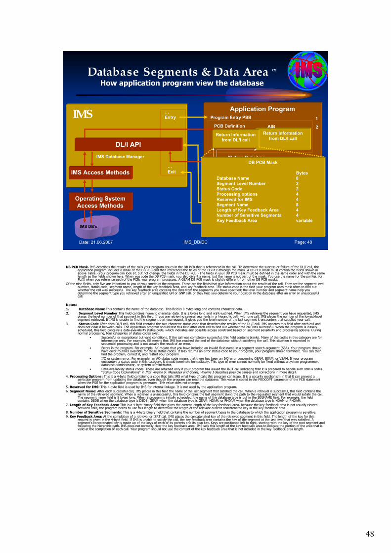
48
IMS_DB/DC Page: 48Date: 21.06.2007
Database Segments & Data Area (2)
How application program view the database
IMS Database Manager
Application Program
IMS Access Methods
Operating System
Access Methods
IMS DB’s
IMS …
Entry Program Entry PSB
Return Information
from DL/I call
PCB Definition AIB
Segment Data Area
IO Area Definition
FUNC, PCB/AIB, IOAREA,(SSA)
DL/I Calls
Program Termination
…
Exit
DL/I API
1
2
3
4
5
DB PCB Mask
Bytes
Database Name 8
Segment Level Number 2
Status Code 2
Processing options 4
Reserved for IMS 4
Segment Name 8
Length of Key Feedback Area 4
Number of Sensitive Segments 4
Key Feedback Area variable
Return Information
from DL/I call
DB PCB Mask. IMS describes the results of the calls your program issues in the DB PCB that is referenced in the call. To determine the success or failure of the DL/I call, the application program includes a mask of the DB PCB and then references the fields of the DB PCB through the mask. A DB PCB mask must contain the fields shown in above Table. (Your program can look at, but not change, the fields in the DB PCB.) The fields in your DB PCB mask must be defined in the same order and with the same length as the fields shown here. When you code the DB PCB mask, you also give it a name, but the name is not part of the mask. You use the name (or the pointer, for PL/I) when you reference each of the PCBs your program processes. A GSAM DB PCB mask is slightly different from other DB PCB masks.
Of the nine fields, only five are important to you as you construct the program. These are the fields that give information about the results of the call. They are the segment level number, status code, segment name, length of the key feedback area, and key feedback area. The status code is the field your program uses most often to find out whether the call was successful. The key feedback area contains the data from the segments you have specified; the level number and segment name help you determine the segment type you retrieved after an unqualified GN or GNP call, or they help you determine your position in the database after an error or unsuccessful call.
Notes:
1. Database Name This contains the name of the database. This field is 8 bytes long and contains character data.
2. Segment Level Number This field contains numeric character data. It is 2 bytes long and right-justified. When IMS retrieves the segment you have requested, IMS places the level number of that segment in this field. If you are retrieving several segments in a hierarchic path with one call, IMS places the number of the lowest-level segment retrieved. If IMS is unable to find the segment that you request, it gives you the level number of the last segment it encounters that satisfied your call.
3. Status Code After each DL/I call, this field contains the two-character status code that describes the results of the DL/I call. IMS updates this field after each call and does not clear it between calls. The application program should test this field after each call to find out whether the call was successful. When the program is initially scheduled, this field contains a data-availability status code, which indicates any possible access constraint based on segment sensitivity and processing options. During normal processing, four categories of status codes exist:
• Successful or exceptional but valid conditions. If the call was completely successful, this field contains blanks. Many of the codes in this category are for information only. For example, GB means that IMS has reached the end of the database without satisfying the call. This situation is expected in sequential processing and is not usually the result of an error.
• Errors in the program. For example, AK means that you have included an invalid field name in a segment search argument (SSA). Your program should have error routines available for these status codes. If IMS returns an error status code to your program, your program should terminate. You can then find the problem, correct it, and restart your program.
• I/O or system error. For example, an AO status code means that there has been an I/O error concerning OSAM, BSAM, or VSAM. If your program encounters a status code in this category, it should terminate immediately. This type of error cannot normally be fixed without a system programmer, database administrator, or system administrator.
• Data-availability status codes. These are returned only if your program has issued the INIT call indicating that it is prepared to handle such status codes. “Status Code Explanations” in IMS Version 9: Messages and Codes, Volume 1 describes possible causes and corrections in more detail.
4. Processing Options: This is a 4-byte field containing a code that tells IMS what type of calls this program can issue. It is a security mechanism in that it can prevent a particular program from updating the database, even though the program can read the database. This value is coded in the PROCOPT parameter of the PCB statement when the PSB for the application program is generated. The value does not change.
5. Reserved for IMS: This 4-byte field is used by IMS for internal linkage. It is not used by the application program.
6. Segment Name: After each successful call, IMS places in this field the name of the last segment that satisfied the call. When a retrieval is successful, this field contains the name of the retrieved segment. When a retrieval is unsuccessful, this field contains the last segment along the path to the requested segment that would satisfy the call. The segment name field is 8 bytes long. When a program is initially scheduled, the name of the database type is put in the SEGNAME field. For example, the field contains DEDB when the database type is DEDB; GSAM when the database type is GSAM; HDAM, or PHDAM when the database type is HDAM or PHDAM.
7. Length of Key Feedback Area: This is a 4-byte binary field that gives the current length of the key feedback area. Because the key feedback area is not usually cleared between calls, the program needs to use this length to determine the length of the relevant current concatenated key in the key feedback area.
8. Number of Sensitive Segments: This is a 4-byte binary field that contains the number of segment types in the database to which the application program is sensitive.
9. Key Feedback Area: At the completion of a retrieval or ISRT call, IMS places the concatenated key of the retrieved segment in this field. The length of the key for this request is given in the 4-byte field. If IMS is unable to satisfy the call, the key feedback area contains the key of the segment at the last level that was satisfied. A segment’s concatenated key is made up of the keys of each of its parents and its own key. Keys are positioned left to right, starting with the key of the root segment and following the hierarchic path. IMS does not normally clear the key feedback area. IMS sets this length of the key feedback area to indicate the portion of the area that is valid at the completion of each call. Your program should not use the content of the key feedback area that is not included in the key feedback area length.
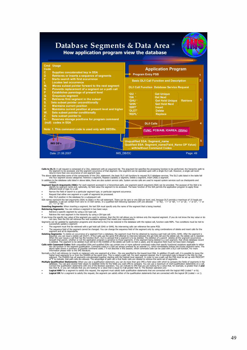
49
IMS_DB/DC Page: 49Date: 21.06.2007
Database Segments & Data Area (3)
How application program view the database
IMS Database Manager
Application Program
IMS Access Methods
Operating System
Access Methods
IMS DB’s
IMS …
Entry Program Entry PSB
Return Information
from DL/I call
PCB Definition AIB
Segment Data Area
IO Area Definition
FUNC, PCB/AIB, IOAREA, (SSAs)
DL/I Calls
Program Termination
…
Exit
DL/I API
1
2
3
4
5Key Feedback Area variable
Return Information
from DL/I call
Basic DL/I Call Function and Description
DL/I Call Function Database Service Request
‘GU ‘ Get Unique
‘GN ‘ Get Next
‘GHU ‘ Get Hold Unique Retrieve
‘GHN ‘ Get Hold Next
‘ISRT’ Insert
‘DLET’ Delete
‘REPL’ Replace
Unqualified SSA: Segment_name
Qualified SSA: Segment_name(Field_Name OP Value)
… with/without Command Codes
Cmd Usage
Code
C Supplies concatenated key in SSA
D Retrieves or inserts a sequence of segments
F Starts search with first occurrence
L Locates last occurrence
M1 Moves subset pointer forward to the next segment
N Prevents replacement of a segment on a path call
P Establishes parentage of present level
Q Enqueues segment
R1 Retrieves first segment in the subset
S1 Sets subset pointer unconditionally
U Maintains current position
V Maintains current position at present level and higher
W1 Sets subset pointer conditionally
Z1 Sets subset pointer to
0 - Reserves storage positions for program command
(null) codes in SSA
Note: 1. This command code is used only with DEDBs.
Calls to DL/I: A call request is composed of a CALL statement with an argument list. The argument list specifies the processing function to be performed, the hierarchic path to the segment to be accessed, and the segment occurrence of that segment. One segment can be operated upon with a single DL/I call. However, a single call never returns more than one occurrence of one segment type.
The above table describes some of the components of the CALL statement: the basic DL/I call functions to request DL/I database services. The DL/I calls listed in the table fall into four segment access categories: Retrieve a segment, Replace (Update) a segment, Delete a segment, insert (Add) a segment.
In addition to the database calls listed in above table, there are also system service calls. System service calls are used to request system services such as checkpoints and restarts.
Segment Search Arguments (SSA): For each segment accessed in a hierarchical path, one segment search argument (SSA) can be provided. The purpose of the SSA is to identify by segment name and, optionally, by field value the segment to be accessed. The basic function of the SSA permits the application program to apply three different kinds of logic to a call:
• Narrow the field of search to a particular segment type, or particular segment occurrence.
• Request that either one segment or a path of segments be processed.
• Alter DL/I position in the database for a subsequent call.
SSA names represent the last arguments (SSA1 to SSAn) in the call statement. There can be zero or one SSA per level, and, because DL/I permits a maximum of 15 levels per database, a call can contain from zero to 15 SSA names. In a qualified SSA following Operators (OP) are allowed: ‘ ‘ or ‘EQ’, ‘>=‘ or ‘GE’, ‘<=‘ or ‘LE’, ‘ >’ or GT’, ‘ <‘ or LT’, ‘<>’ or ‘NE’.
Inserting Segments: When inserting a segment, the last SSA must specify only the name of the segment that is being inserted.
Retrieving Segments: You can retrieve a segment in two basic ways:
• Retrieve a specific segment by using a GU type call,
• Retrieve the next segment in the hierarchy by using a GN type call.
If you know the specific key value of the segment you want to retrieve, then the GU call allows you to retrieve only the required segment. If you do not know the key value or do not care, then the GN call retrieves the next available segment that meets your requirements.
Segments can be updated by application programs and returned to DL/I to be restored in the database with the replace call, function code REPL. Two conditions must be met to successfully update a segment:
• The segment must first be retrieved with a get hold call (GHU or GHN). No intervening calls can reference the same PCB.
• The sequence field of the segment cannot be changed. You can change the sequence field of the segment only by using combinations of delete and insert calls for the segment and all its dependents.
Deleting Segments: To delete an occurrence of a segment from a database, the segment must first be obtained by issuing a get hold call (GHU, GHN). After the segment is acquired, you can issue a delete call (DLET). If DL/I calls use the same PCB attempt to intervene between the get hold call and the delete call, the delete call is rejected. When the user issues a call that has the function DLET, DL/I is advised that a segment is to be deleted. The deletion of a parent deletes all the segment occurrences beneath that parent, whether or not the application program is sensitive to those segments. If the segment being deleted is a root segment, that whole database record is deleted. The segment to be deleted must still be in the IOAREA of the delete call (with no SSA is used), and its sequence field must not have been changed.
Calls with Command Codes: Both unqualified SSAs and qualified SSAs can contain one or more optional command codes that specify functional variations applicable to either the call function or the segment qualification. Command codes in a SSA are always prefixed by an asterisk (*), which immediately follows the 8-byte segment name. The above table shows a summary of possible command codes. I ‘ll not describe in this session, which command code can be used with a DL/I call function. For more information please refer to the IMS literature.
Normally a DL/I call retrieves (or inserts or replaces) only one segment at a time – the one specified by the lowest level SSA. In addition (D-path call), it is possible to move the higher level segments to or from the IOAREA at the same time. This is called a path call. For each segment desired, the D command code is placed in the SSA for that segment. The IOAREA has all segments concatenated together starting with the highest level segment. In order to use a path call the PSB must be set up with PROCOPT of ‘P’ to indicate, that path calls are allowed. The advantage of path call is that fewer calls are needed to retrieve the same set of segments.
Multiple Qualification Statements: When you use a qualification statement, you can do more than give IMS a field value with which to compare the fields of segments in the database. You can give several field values to establish limits for the fields you want IMS to compare. You can use a maximum of 1024 qualification statements on a call. Connect the qualification statements with one of the Boolean operators. You can indicate to IMS that you are looking for a value that, for example, is greater than A and less than B, or you can indicate that you are looking for a value that is equal to A or greater than B. The Boolean operators are:
• Logical AND For a segment to satisfy this request, the segment must satisfy both qualification statements that are connected with the logical AND (coded * or &).
• Logical OR For a segment to satisfy this request, the segment can satisfy either of the qualification statements that are connected with the logical OR (coded + or |).
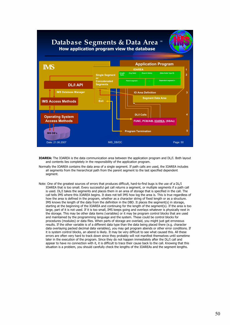
50
IMS_DB/DC Page: 50Date: 21.06.2007
Database Segments & Data Area (4)
How application program view the database
IMS Database Manager
Application Program
IMS Access Methods
Operating System
Access Methods
IMS DB’s
IMS …
Entry Program Entry PSB
Return Information
from DL/I call
PCB Definition AIB
Segment Data Area
IO Area Definition
FUNC, PCB/AIB, IOAREA, (SSAs)
DL/I Calls
Program Termination
…
Exit
DL/I API
1
2
3
4
5
Return Information
from DL/I call
IOAREA
(length
field)
(Key field) (Search fields) (Data fields Type B)
Parent segment Dependent segment n…
Single Segment
or
Concatenated
Segments
IOAREA: The IOAREA is the data communication area between the application program and DL/I. Both layout and contents lies completely in the responsibility of the application program.
Normally the IOAREA contains the data area of a single segment. If path calls are used, the IOAREA includes all segments from the hierarchical path from the parent segment to the last specified dependent segment.
Note: One of the greatest sources of errors that produces difficult, hard-to-find bugs is the use of a DL/I IOAREA that is too small. Every successful get call returns a segment, or multiple segments if a path call is used. DL/I takes the segments and places them in an area of storage that is specified in the call. The call tells IMS where this IOAREA begins. It does not tell IMS how log the area is. This is true regardless of how the area is defined in the program, whether as a character string of fixed length or as a structure. IMS knows the length of the data from the definition in the DBD. It places the segment(s) in storage, starting at the beginning of the IOAREA and continuing for the length of the segment(s). If the area is too large, part of it is not used. If it is too small, IMS keeps going and overlays whatever is physically next in the storage. This may be other data items (variables) or it may be program control blocks that are used and maintained by the programming language and the system. These could be control blocks for procedures (modules) or data files. When parts of storage are overlaid, you might just get erroneous results. If the other variable is of a different data type than the data being placed there (e.g. character data overlaying packed decimal data variables), you may get program abends or other error conditions. If it is system control blocks, an abend is likely. It may be very difficult to see what caused this. All these errors are often very hard to track down since they probably will not manifest themselves until sometime later in the execution of the program. Since they do not happen immediately after the DL/I call and appear to have no connection with it, it is difficult to trace their cause back to the call. Knowing that this situation is a problem, you should carefully check the lengths of the IOAREAs and the segment lengths.
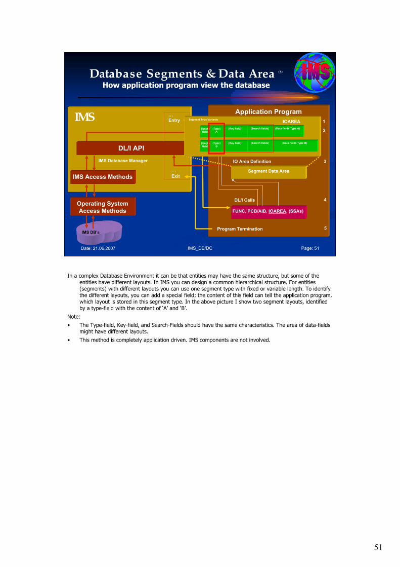
51
IMS_DB/DC Page: 51Date: 21.06.2007
Database Segments & Data Area (5)
How application program view the database
IMS Database Manager
Application Program
IMS Access Methods
Operating System
Access Methods
IMS DB’s
IMS …
Entry Program Entry PSB
Return Information
from DL/I call
PCB Definition AIB
Segment Data Area
IO Area Definition
FUNC, PCB/AIB, IOAREA, (SSAs)
DL/I Calls
Program Termination
…
Exit
DL/I API
1
2
3
4
5
Return Information
from DL/I call
IOAREA
(length
field)
(Type)
A
(Key field) (Search fields) (Data fields Type A)
(length
field)
(Type)
B
(Key field) (Search fields) (Data fields Type B)
Segment Type Variants
In a complex Database Environment it can be that entities may have the same structure, but some of the entities have different layouts. In IMS you can design a common hierarchical structure. For entities (segments) with different layouts you can use one segment type with fixed or variable length. To identify the different layouts, you can add a special field; the content of this field can tell the application program, which layout is stored in this segment type. In the above picture I show two segment layouts, identified by a type-field with the content of ‘A’ and ‘B’.
Note:
• The Type-field, Key-field, and Search-Fields should have the same characteristics. The area of data-fields might have different layouts.
• This method is completely application driven. IMS components are not involved.
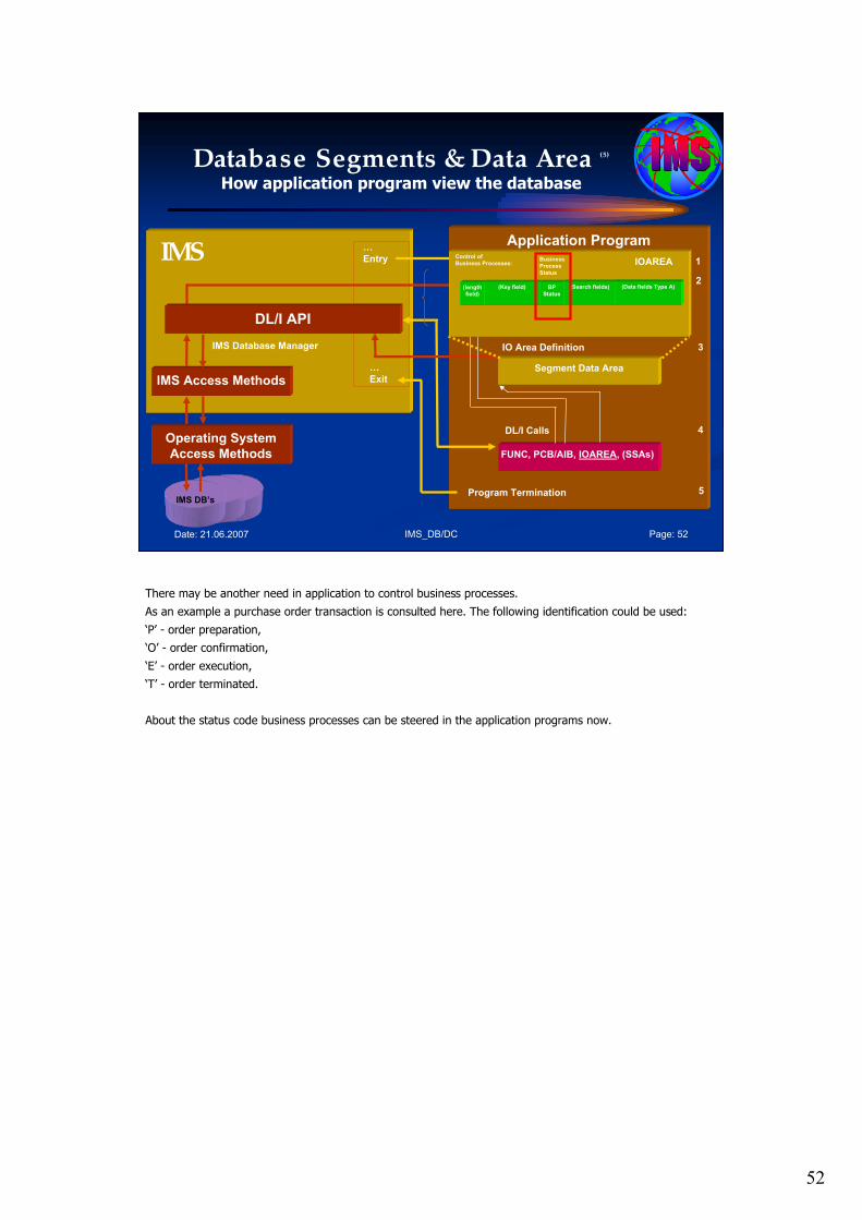
52
IMS_DB/DC Page: 52Date: 21.06.2007
Database Segments & Data Area (5)
How application program view the database
IMS Database Manager
Application Program
IMS Access Methods
Operating System
Access Methods
IMS DB’s
IMS …
Entry Program Entry PSB
Return Information
from DL/I call
PCB Definition AIB
Segment Data Area
IO Area Definition
FUNC, PCB/AIB, IOAREA, (SSAs)
DL/I Calls
Program Termination
…
Exit
DL/I API
1
2
3
4
5
Return Information
from DL/I call
IOAREA
(length
field)
Business
Process
Status
(Key field) BP
Status
(Search fields) (Data fields Type A)
Control of
Business Processes:
There may be another need in application to control business processes.
As an example a purchase order transaction is consulted here. The following identification could be used:
‘P’ - order preparation,
‘O’ - order confirmation,
‘E’ - order execution,
‘T’ - order terminated.
About the status code business processes can be steered in the application programs now.
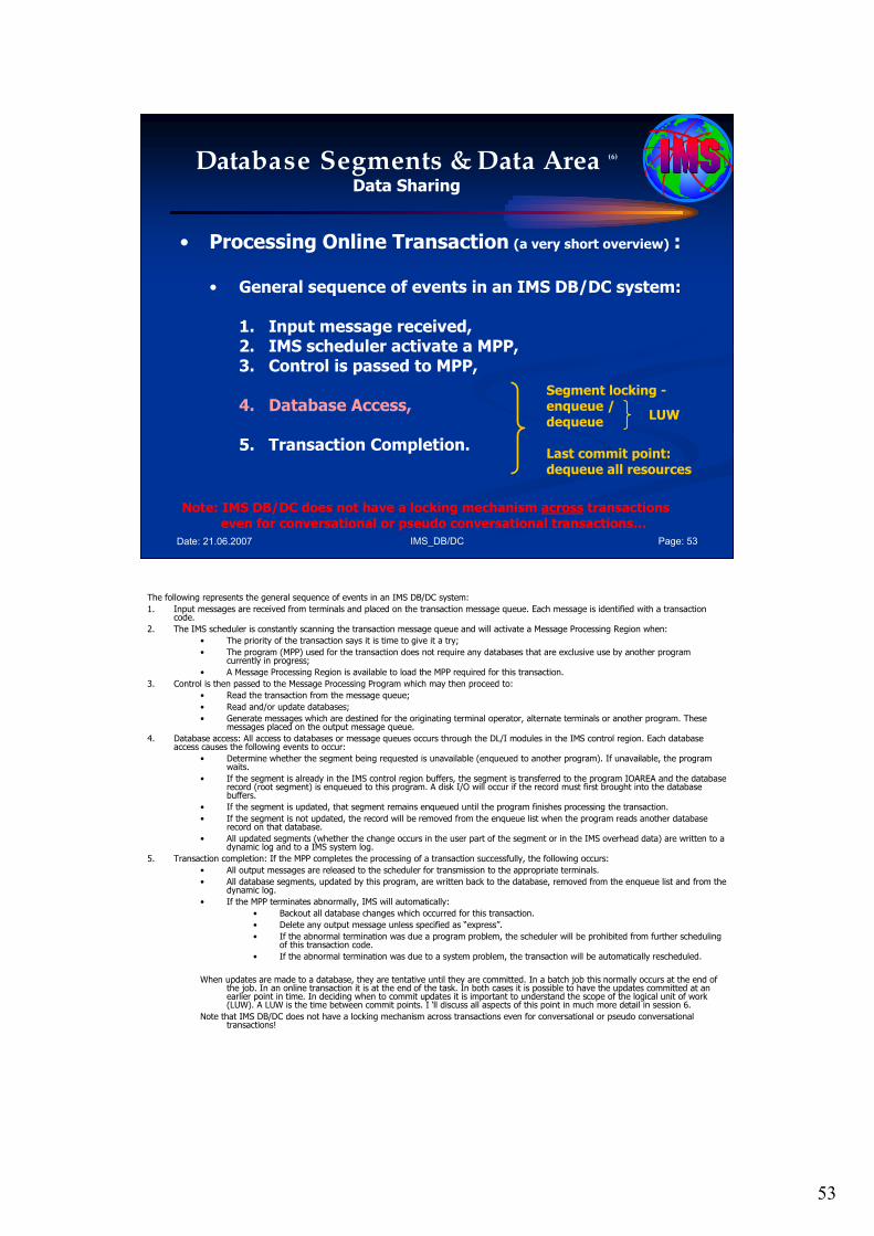
53
IMS_DB/DC Page: 53Date: 21.06.2007
Database Segments & Data Area (6)
Data Sharing
• Processing Online Transaction (a very short overview) :
• General sequence of events in an IMS DB/DC system:
1. Input message received,2. IMS scheduler activate a MPP,3. Control is passed to MPP,
4. Database Access,
5. Transaction Completion.
Note: IMS DB/DC does not have a locking mechanism across transactionseven for conversational or pseudo conversational transactions…
Segment locking -enqueue /dequeue
Last commit point:dequeue all resources
LUW
The following represents the general sequence of events in an IMS DB/DC system:
1. Input messages are received from terminals and placed on the transaction message queue. Each message is identified with a transaction code.
2. The IMS scheduler is constantly scanning the transaction message queue and will activate a Message Processing Region when:
• The priority of the transaction says it is time to give it a try;
• The program (MPP) used for the transaction does not require any databases that are exclusive use by another program currently in progress;
• A Message Processing Region is available to load the MPP required for this transaction.
3. Control is then passed to the Message Processing Program which may then proceed to:
• Read the transaction from the message queue;
• Read and/or update databases;
• Generate messages which are destined for the originating terminal operator, alternate terminals or another program. These messages placed on the output message queue.
4. Database access: All access to databases or message queues occurs through the DL/I modules in the IMS control region. Each database access causes the following events to occur:
• Determine whether the segment being requested is unavailable (enqueued to another program). If unavailable, the program waits.
• If the segment is already in the IMS control region buffers, the segment is transferred to the program IOAREA and the database record (root segment) is enqueued to this program. A disk I/O will occur if the record must first brought into the database buffers.
• If the segment is updated, that segment remains enqueued until the program finishes processing the transaction.
• If the segment is not updated, the record will be removed from the enqueue list when the program reads another database record on that database.
• All updated segments (whether the change occurs in the user part of the segment or in the IMS overhead data) are written to a dynamic log and to a IMS system log.
5. Transaction completion: If the MPP completes the processing of a transaction successfully, the following occurs:
• All output messages are released to the scheduler for transmission to the appropriate terminals.
• All database segments, updated by this program, are written back to the database, removed from the enqueue list and from the dynamic log.
• If the MPP terminates abnormally, IMS will automatically:
• Backout all database changes which occurred for this transaction.
• Delete any output message unless specified as “express”.
• If the abnormal termination was due a program problem, the scheduler will be prohibited from further scheduling of this transaction code.
• If the abnormal termination was due to a system problem, the transaction will be automatically rescheduled.
When updates are made to a database, they are tentative until they are committed. In a batch job this normally occurs at the end of the job. In an online transaction it is at the end of the task. In both cases it is possible to have the updates committed at anearlier point in time. In deciding when to commit updates it is important to understand the scope of the logical unit of work (LUW). A LUW is the time between commit points. I ‘ll discuss all aspects of this point in much more detail in session 6.
Note that IMS DB/DC does not have a locking mechanism across transactions even for conversational or pseudo conversational transactions!
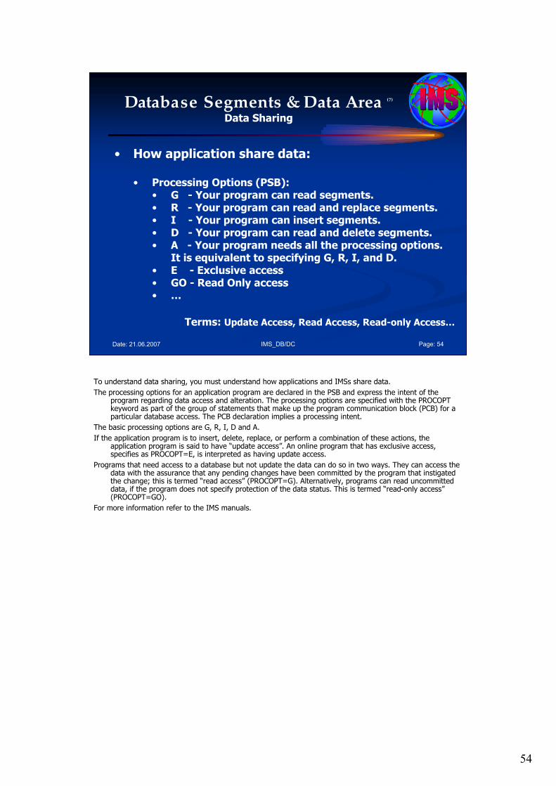
54
IMS_DB/DC Page: 54Date: 21.06.2007
Database Segments & Data Area (7)
Data Sharing
• How application share data:
• Processing Options (PSB):• G - Your program can read segments. • R - Your program can read and replace segments. • I - Your program can insert segments. • D - Your program can read and delete segments. • A - Your program needs all the processing options.
It is equivalent to specifying G, R, I, and D.• E - Exclusive access• GO - Read Only access• …
Terms: Update Access, Read Access, Read-only Access…
To understand data sharing, you must understand how applications and IMSs share data.
The processing options for an application program are declared in the PSB and express the intent of the program regarding data access and alteration. The processing options are specified with the PROCOPT keyword as part of the group of statements that make up the program communication block (PCB) for a particular database access. The PCB declaration implies a processing intent.
The basic processing options are G, R, I, D and A.
If the application program is to insert, delete, replace, or perform a combination of these actions, the application program is said to have “update access”. An online program that has exclusive access, specifies as PROCOPT=E, is interpreted as having update access.
Programs that need access to a database but not update the data can do so in two ways. They can access the data with the assurance that any pending changes have been committed by the program that instigated the change; this is termed “read access” (PROCOPT=G). Alternatively, programs can read uncommitted data, if the program does not specify protection of the data status. This is termed “read-only access”(PROCOPT=GO).
For more information refer to the IMS manuals.
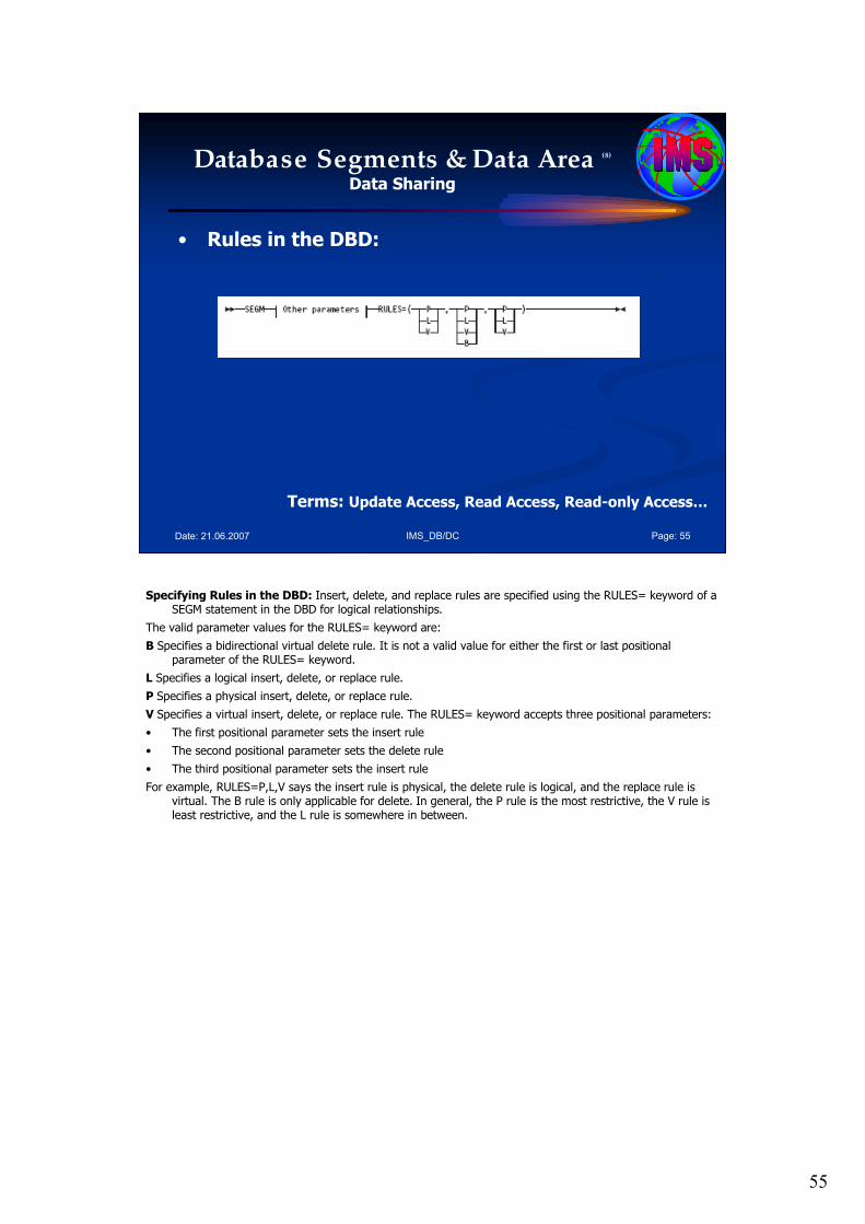
55
IMS_DB/DC Page: 55Date: 21.06.2007
Database Segments & Data Area (8)
Data Sharing
• Rules in the DBD:
Terms: Update Access, Read Access, Read-only Access…
Specifying Rules in the DBD: Insert, delete, and replace rules are specified using the RULES= keyword of a SEGM statement in the DBD for logical relationships.
The valid parameter values for the RULES= keyword are:
B Specifies a bidirectional virtual delete rule. It is not a valid value for either the first or last positional parameter of the RULES= keyword.
L Specifies a logical insert, delete, or replace rule.
P Specifies a physical insert, delete, or replace rule.
V Specifies a virtual insert, delete, or replace rule. The RULES= keyword accepts three positional parameters:
• The first positional parameter sets the insert rule
• The second positional parameter sets the delete rule
• The third positional parameter sets the insert rule
For example, RULES=P,L,V says the insert rule is physical, the delete rule is logical, and the replace rule is virtual. The B rule is only applicable for delete. In general, the P rule is the most restrictive, the V rule is least restrictive, and the L rule is somewhere in between.
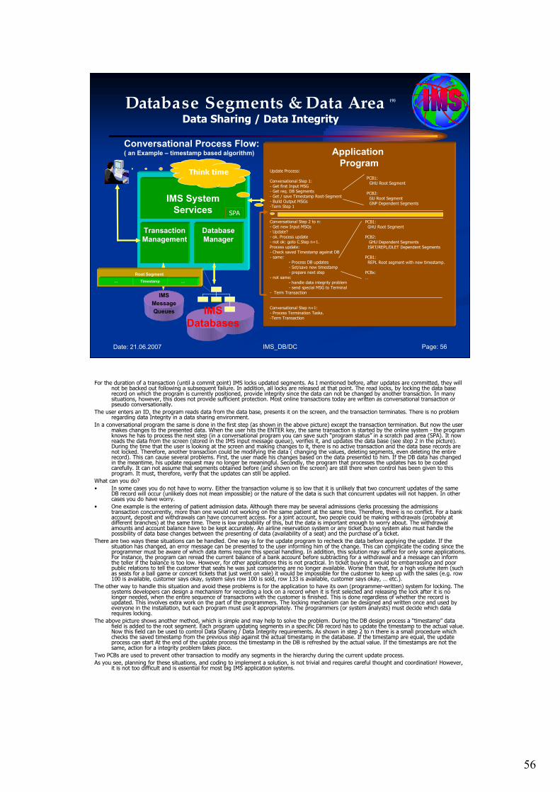
56
IMS_DB/DC Page: 56Date: 21.06.2007
Database Segments & Data Area (9)
Data Sharing / Data Integrity
Conversational Process Flow:( an Example – timestamp based algorithm)
IMS System
Services
Transaction
Management
Database
Manager
IMS
Message
Queues IMS
Databases
SPA
Application
ProgramUpdate Process:
Conversational Step 1:- Get first Input MSG- Get req. DB Segments- Get / save Timestamp Root-Segment- Build Output MSGs-Term Step 1
Conversational Step 2 to n:- Get new Input MSGs- Update?- ok. Process update - not ok: goto C.Step n+1.Process update:- Check saved Timestamp against DB - same:
- Process DB updates- Set/save new timestamp- prepare next step
- not same: - handle data integrity problem- send special MSG to Terminal
- Term Transaction
Conversational Step n+1:- Process Termination Tasks. -Term Transaction
PCB1:GHU Root Segment
PCB2:GU Root SegmentGNP Dependent Segments
PCB1:GHU Root Segment
PCB2:GHU Dependent SegmentsISRT/REPL/DLET Dependent Segments
PCB1:REPL Root segment with new timestamp.
PCBx:…
Root Segment
… Timestamp …
Think time
For the duration of a transaction (until a commit point) IMS locks updated segments. As I mentioned before, after updates are committed, they will not be backed out following a subsequent failure. In addition, all locks are released at that point. The read locks, by locking the data base record on which the program is currently positioned, provide integrity since the data can not be changed by another transaction. In many situations, however, this does not provide sufficient protection. Most online transactions today are written as conversational transaction or pseudo conversationally.
The user enters an ID, the program reads data from the data base, presents it on the screen, and the transaction terminates. There is no problem regarding data Integrity in a data sharing environment.
In a conversational program the same is done in the first step (as shown in the above picture) except the transaction termination. But now the user makes changes to the presented data. When the user hits the ENTER key, the same transaction is started by the online system - the program knows he has to process the next step (in a conversational program you can save such “program status” in a scratch pad area (SPA). It now reads the data from the screen (stored in the IMS input message queue), verifies it, and updates the data base (see step 2 in the picture). During the time that the user is looking at the screen and making changes to it, there is no active transaction and the data base records are not locked. Therefore, another transaction could be modifying the data ( changing the values, deleting segments, even deleting the entire record). This can cause several problems. First, the user made his changes based on the data presented to him. If the DB data has changed in the meantime, his update request may no longer be meaningful. Secondly, the program that processes the updates has to be coded carefully. It can not assume that segments obtained before (and shown on the screen) are still there when control has been given to this program. It must, therefore, verify that the updates can still be applied.
What can you do?
• In some cases you do not have to worry. Either the transaction volume is so low that it is unlikely that two concurrent updates of the same DB record will occur (unlikely does not mean impossible) or the nature of the data is such that concurrent updates will not happen. In other cases you do have worry.
• One example is the entering of patient admission data. Although there may be several admissions clerks processing the admissionstransaction concurrently, more than one would not working on the same patient at the same time. Therefore, there is no conflict. For a bank account, deposit and withdrawals can have concurrent access. For a joint account, two people could be making withdrawals (probably at different branches) at the same time. There is low probability of this, but the data is important enough to worry about. The withdrawal amounts and account balance have to be kept accurately. An airline reservation system or any ticket buying system also must handle the possibility of data base changes between the presenting of data (availability of a seat) and the purchase of a ticket.
There are two ways these situations can be handled. One way is for the update program to recheck the data before applying the update. If the situation has changed, an error message can be presented to the user informing him of the change. This can complicate the coding since the programmer must be aware of which data items require this special handling. In addition, this solution may suffice for only some applications. For instance, the program can reread the current balance of a bank account before subtracting for a withdrawal and a message can inform the teller if the balance is too low. However, for other applications this is not practical. In ticket buying it would be embarrassing and poor public relations to tell the customer that seats he was just considering are no longer available. Worse than that, for a high volume item (such as seats for a ball game or concert tickets that just went on sale) it would be impossible for the customer to keep up with the sales (e.g. row 100 is available, customer says okay, system says row 100 is sold, row 133 is available, customer says okay, … etc.).
The other way to handle this situation and avoid these problems is for the application to have its own (programmer-written) system for locking. The systems developers can design a mechanism for recording a lock on a record when it is first selected and releasing the lock after it is no longer needed, when the entire sequence of transactions with the customer is finished. This is done regardless of whether the record is updated. This involves extra work on the part of the programmers. The locking mechanism can be designed and written once and used by everyone in the installation, but each program must use it appropriately. The programmers (or system analysts) must decide which data requires locking.
The above picture shows another method, which is simple and may help to solve the problem. During the DB design process a “timestamp” data field is added to the root segment. Each program updating segments in a specific DB record has to update the timestamp to the actual value. Now this field can be used to control Data Sharing / Data Integrity requirements. As shown in step 2 to n there is a small procedure which checks the saved timestamp from the previous step against the actual timestamp in the database. If the timestamp are equal, the update process can start At the end of the update process the timestamp in the DB is refreshed by the actual value. If the timestamps are not the same, action for a integrity problem takes place.
Two PCBs are used to prevent other transaction to modify any segments in the hierarchy during the current update process.
As you see, planning for these situations, and coding to implement a solution, is not trivial and requires careful thought and coordination! However, it is not too difficult and is essential for most big IMS application systems.
57
IMS_DB/DC Page: 57Date: 21.06.2007
Database Segments & Data Area (10)
Data Compression
•Terms:
• Segment Edit/Compression Routines• saves space on DASD,• doesn’t affect view of the segment by application program• use of compression is a trade-off between storage, I/Os and CPU processing• Key Compression vs. Data Compression
You may compress segments by using Segment Edit/Compression Routines. This reduces the amount of space that is required on DASD for the segments. It does not affect the view of the segments by the application programs. You may use compression with PHDAM, PHIDAM, HISAM, HDAM, and HIDAM databases. You cannot use compression with PSINDEX, SHISAM, or INDEX databases.
You specify compression with the COMPRTN parameter on the SEGM statement in the DBD. You may use different specifications for different segment types. You may compress some segment types in a database while not compression others. You may use different compression routines for different segment types.
The use of compression is a trade-off between storage, I/Os and CPU processing.• Key Compression vs. Data Compression: If you implement compression, you have the option to
specifying whether you want key compression or only data compression. With key compression the entire segment past the prefix is compressed. With data compression only the data following the key is compressed. Key compression cannot be used with HISAM root segments. They must use data compression. The compression option you choose should depend on the amount of potential savings from key compression versus the extra processing it requires. This depends on the size of the key, the location of the key in the segment, and the type of processing done against the segment.
58
IMS_DB/DC Page: 58Date: 21.06.2007
Agenda Session 2: Database Basics
1. Basic Terms
2. Physical Database
3. Logical Database / Relationships
4. Secondary Indexes
5. How data is stored/retrieved in a DB
6. DB Records, Segments, Pointers
7. Database Segments & Data Area
8. Points not addressed
8. Database Segments & Data Area
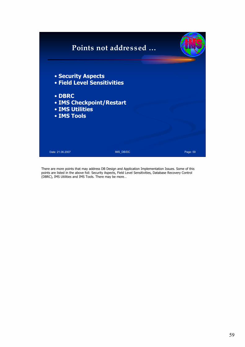
59
IMS_DB/DC Page: 59Date: 21.06.2007
Points not addressed …
• Security Aspects• Field Level Sensitivities
• DBRC• IMS Checkpoint/Restart• IMS Utilities• IMS Tools
There are more points that may address DB Design and Application Implementation Issues. Some of this points are listed in the above foil: Security Aspects, Field Level Sensitivities, Database Recovery Control (DBRC), IMS Utilities and IMS Tools. There may be more…

60
IMS_DB/DC Page: 60Date: 21.06.2007
Source
See: • IBM Web page
http://www-306.ibm.com/software/data/ims/
• BookAn Introduction to IMS, IBM Press
In all sessions I like to motivate you to study additional books and publications about IMS DB/DC.

61
Date: 21.06.2007 IMS_03_2.ppt Page: 61
Questions / CommentsQuestions / Comments……
? ? ?? ? ?
Questions, comments, further information?
Please feel free to e-mail me!
Dipl.Ing. Werner HoffmannDipl.Ing. Werner Hoffmann
EMAIL: EMAIL: pwhoffmann@[email protected]
The time for this session is over. If you have additional questions or comments or like to get further information please feel free to e mail me at [email protected].

62
IMS_DB/DC Page: 62Date: 21.06.2007
Workshop
The world depends on it
The End…
Part III/2: IMS Hierarchical Database Model IMS Hierarchical Database Model
BasicsBasics
I hope this presentation was right for you! Enjoy the following discussion!
1
Date: 21.06.2007 IMS_03_3.ppt Page: 1
IBM Mainframe
IMS DB/DC
Database Design Workshop
Part III: Part III:
IMS Hierarchical Database ModelIMS Hierarchical Database ModelSession 3: Session 3: Hierarchical Access MethodsHierarchical Access Methods
April 2007 April 2007 –– 2nd Version2nd Version
presented bypresented by
Dipl. Dipl. IngIng. Werner Hoffmann. Werner HoffmannEMAIL: EMAIL: pwhoffmann @ tpwhoffmann @ t--online.deonline.de
A member of IEEE and ACM
Mainframe
Please see the notes pages for additional comments. Please see the notes pages for additional comments.
Welcome to the workshop called “IMS DB/DC". This is part 3: IMS Hierarchical Database Model – Session 3: Hierarchical Access Methods.
2
IMS_DB/DC Page: 2Date: 21.06.2007
Agenda Session 3: Hierarchical Access Methods
1. HD DatabasesHDAM & HIDAM Access MethodPHDAM & PHIDAM Access Methods
2. Index Databases3. Fast Path DEDBs4. GSAM Access Method5. HS Databases
HSAM & HISAM Access Method
6. Operating System Access Methods7. Data Set Groups8. Summary
Here is the Agenda for the IMS DB/DC workshop part III/3: Hierarchical Access Methods.
In this session I like to speak about:
1. HDAM Access Method
2. HIDAM Access Method
3. PHDAM and PHIDAM Access Methods
4. Index Databases
5. Fast Path DEDBs
6. GSAM Access Method
7. HSAM and HISAM Access Method
8. Operating System Access Methods
9. Data Set Groups

3
IMS_DB/DC Page: 3Date: 21.06.2007
Agenda Session 3: Hierarchical Access Methods
1. HD Databases• HDAM & HIDAM Access Method
• PHDAM & PHIDAM Access Methods
2. Index Databases
3. Fast Path DEDBs
4. GSAM Access Method
5. HS Databases
• HSAM & HISAM Access Method
6. Operating System Access Methods
7. Data Set Groups
8. Summary
1. HD Databases.
4
IMS_DB/DC Page: 4Date: 21.06.2007
HD Databases (1)
HD databases share these characteristics:
• Pointers are used to relate segments.• Deleted segments are physically removed.• VSAM ESDS or OSAM data sets are used for storage.• HD databases are stored on DASD.• HD databases are of a more complex organization than sequentially organized databases.
Hierarchic Direct Databases: Hierarchic direct access method (HDAM) and hierarchic indexed direct access method (HIDAM) databases are referred to collectively as HD databases. The hierarchic direct databases were developed to overcome some of the deficiencies of sequential access databases. HD databases share these characteristics:
• Pointers are used to relate segments.
• Deleted segments are physically removed.
• VSAM ESDS or OSAM data sets are used for storage.
• HD databases are stored on DASD.
• HD databases are of a more complex organization than sequentially organized databases.
The following sections discuss HDAM, PHDAM, HIDAM and PHIDAM database organizations. Because pointers play such an integral role in direct access databases, they are referenced frequently in the text. Pointers are four-byte address values that give the offset from the beginning of the data set of the segment being addressed. They tie the segments together without the need for segments to be physically adjacent. Segments can be inserted or deleted without the need to move other segments.
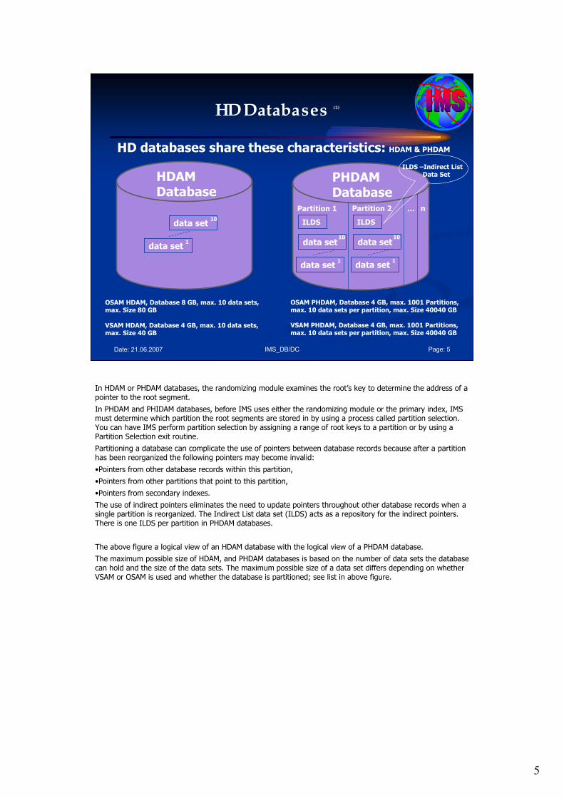
5
IMS_DB/DC Page: 5Date: 21.06.2007
HD Databases (2)
HD databases share these characteristics: HDAM & PHDAM
HDAMDatabase
PHDAMDatabase
data set1
data set10
data set1
data set10
ILDS
Partition 1
data set1
data set10
ILDS
Partition 2 n…
OSAM HDAM, Database 8 GB, max. 10 data sets,max. Size 80 GB
VSAM HDAM, Database 4 GB, max. 10 data sets,max. Size 40 GB
OSAM PHDAM, Database 4 GB, max. 1001 Partitions, max. 10 data sets per partition, max. Size 40040 GB
VSAM PHDAM, Database 4 GB, max. 1001 Partitions, max. 10 data sets per partition, max. Size 40040 GB
ILDS –Indirect ListData Set
In HDAM or PHDAM databases, the randomizing module examines the root’s key to determine the address of a pointer to the root segment.
In PHDAM and PHIDAM databases, before IMS uses either the randomizing module or the primary index, IMS must determine which partition the root segments are stored in by using a process called partition selection. You can have IMS perform partition selection by assigning a range of root keys to a partition or by using a Partition Selection exit routine.
Partitioning a database can complicate the use of pointers between database records because after a partition has been reorganized the following pointers may become invalid:
•Pointers from other database records within this partition,
•Pointers from other partitions that point to this partition,
•Pointers from secondary indexes.
The use of indirect pointers eliminates the need to update pointers throughout other database records when a single partition is reorganized. The Indirect List data set (ILDS) acts as a repository for the indirect pointers. There is one ILDS per partition in PHDAM databases.
The above figure a logical view of an HDAM database with the logical view of a PHDAM database.
The maximum possible size of HDAM, and PHDAM databases is based on the number of data sets the database can hold and the size of the data sets. The maximum possible size of a data set differs depending on whether VSAM or OSAM is used and whether the database is partitioned; see list in above figure.
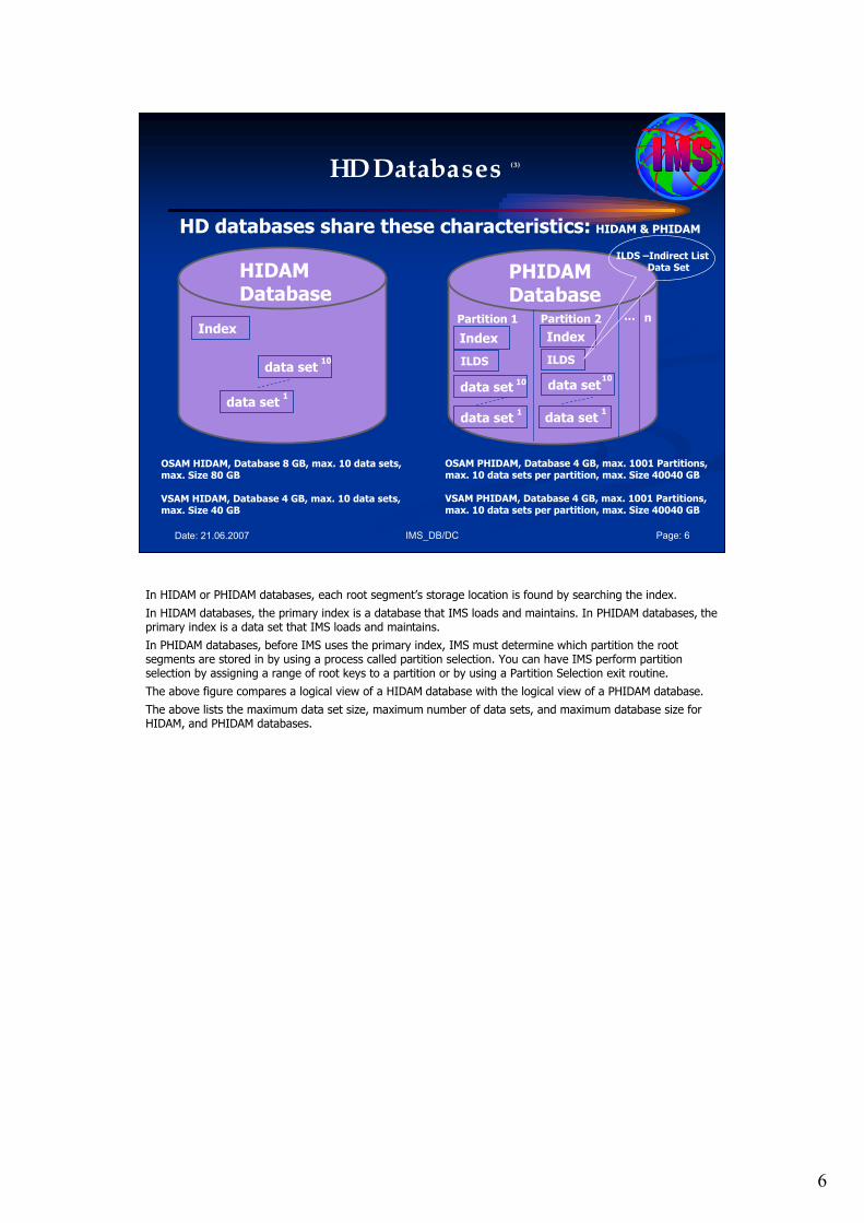
6
IMS_DB/DC Page: 6Date: 21.06.2007
HD Databases (3)
HD databases share these characteristics: HIDAM & PHIDAM
OSAM HIDAM, Database 8 GB, max. 10 data sets,max. Size 80 GB
VSAM HIDAM, Database 4 GB, max. 10 data sets,max. Size 40 GB
OSAM PHIDAM, Database 4 GB, max. 1001 Partitions, max. 10 data sets per partition, max. Size 40040 GB
VSAM PHIDAM, Database 4 GB, max. 1001 Partitions, max. 10 data sets per partition, max. Size 40040 GB
HIDAMDatabase
PHIDAMDatabase
data set1
data set10
data set1
data set10
ILDS
Partition 1
data set1
data set10
ILDS
Partition 2 n…Index
Index Index
ILDS –Indirect ListData Set
In HIDAM or PHIDAM databases, each root segment’s storage location is found by searching the index.
In HIDAM databases, the primary index is a database that IMS loads and maintains. In PHIDAM databases, the primary index is a data set that IMS loads and maintains.
In PHIDAM databases, before IMS uses the primary index, IMS must determine which partition the root segments are stored in by using a process called partition selection. You can have IMS perform partition selection by assigning a range of root keys to a partition or by using a Partition Selection exit routine.
The above figure compares a logical view of a HIDAM database with the logical view of a PHIDAM database.
The above lists the maximum data set size, maximum number of data sets, and maximum database size for HIDAM, and PHIDAM databases.
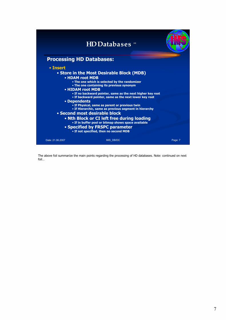
7
IMS_DB/DC Page: 7Date: 21.06.2007
HD Databases (4)
Processing HD Databases:
• Insert• Store in the Most Desirable Block (MDB)
• HDAM root MDB• The one which is selected by the randomizer• The one containing its previous synonym
• HIDAM root MDB• If no backward pointer, same as the next higher key root• If backward pointer, same as the next lower key root
• Dependents• If Physical, same as parent or previous twin• If Hierarchic, same as previous segment in hierarchy
• Second most desirable block• Nth Block or CI left free during loading
• If in buffer pool or bitmap shows space available
• Specified by FRSPC parameter• If not specified, then no second MDB
The above foil summarize the main points regarding the processing of HD databases. Note: continued on next foil…

8
IMS_DB/DC Page: 8Date: 21.06.2007
HD Databases (5)
Processing HD Databases:• Delete
• The segment and all of its dependents are removed • FSE is used indicate the space is free
• Create a new FSE and update the FSAP/FSE Chain• Update length field of preceding FSE
• Pointers are updated• Replace
• No change in length or fixed-length• Overwrite old segment with updated segment
• Shorter segment• Space previously occupied is freed• FSE created if at least 8 bytes shorter
• Longer segment• If adjacent free space lets it fit, store in original location• If no space available, separated data
Data part goes to overflow with prefix of SC and DB=x'FF'Bit 4 of DB in original prefix is turned onPointer to data in overflow is built after prefixRemainder of space is freed
Continued: The above foil summarize the main points regarding the processing of HD databases.

9
IMS_DB/DC Page: 9Date: 21.06.2007
HD Databases (6)
HD Space Management
HD Space Search Algorithm:
• In the MDB (this will be in the buffer pool)• In the second MDB• Any block in the buffer pool on the same cylinder• Any block on the same track
• If the bitmap shows space available
• Any block on the same cylinder• If the bitmap shows space available
• Any block in the buffer pool within +/-SCAN cylinders• Any block within +/-SCAN cylinders
• If the bitmap shows space available
• Any block at the end of the data set is in the pool• Any block at the end of the data set
• If the bitmap shows space available• Extend the data set if necessary
• Any block where the bitmap shows space
MDB - Most Desirable Block
The above foil describe the HD space search algorithm.
10
IMS_DB/DC Page: 10Date: 21.06.2007
Agenda Session 3: Hierarchical Access Methods
1. HD Databases• HDAM & HIDAM Access Method
• PHDAM & PHIDAM Access Methods
2. Index Databases
3. Fast Path DEDBs
4. GSAM Access Method
5. HS Databases
• HSAM & HISAM Access Method
6. Operating System Access Methods
7. Data Set Groups
8. Summary
HIDAM Access Method.
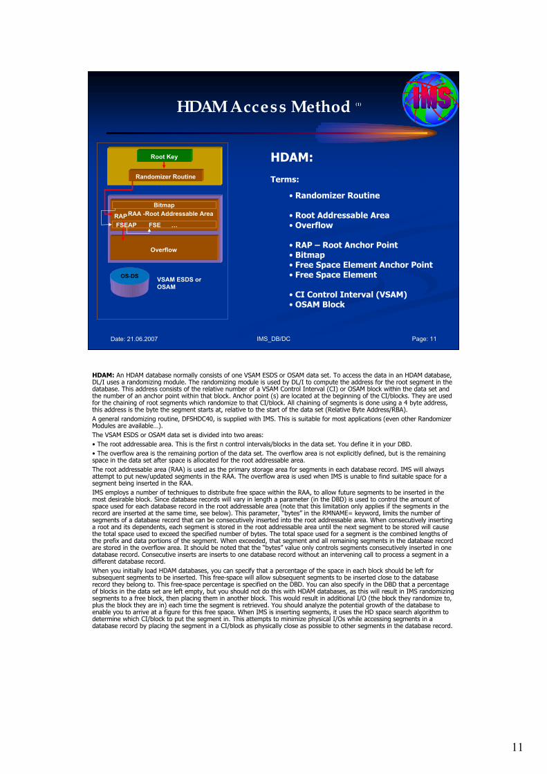
11
IMS_DB/DC Page: 11Date: 21.06.2007
HDAM Access Method (1)
HDAM:
Terms:
• Randomizer Routine
• Root Addressable Area• Overflow
• RAP – Root Anchor Point• Bitmap• Free Space Element Anchor Point• Free Space Element
• CI Control Interval (VSAM)• OSAM Block
Root Key
Randomizer Routine
RAA -Root Addressable Area
Overflow
OS-DSVSAM ESDS or
OSAM
RAP
Bitmap
FSEAP FSE …
HDAM: An HDAM database normally consists of one VSAM ESDS or OSAM data set. To access the data in an HDAM database, DL/I uses a randomizing module. The randomizing module is used by DL/I to compute the address for the root segment in the database. This address consists of the relative number of a VSAM Control Interval (CI) or OSAM block within the data set and the number of an anchor point within that block. Anchor point (s) are located at the beginning of the CI/blocks. They are used for the chaining of root segments which randomize to that CI/block. All chaining of segments is done using a 4 byte address, this address is the byte the segment starts at, relative to the start of the data set (Relative Byte Address/RBA).
A general randomizing routine, DFSHDC40, is supplied with IMS. This is suitable for most applications (even other Randomizer Modules are available…).
The VSAM ESDS or OSAM data set is divided into two areas:
• The root addressable area. This is the first n control intervals/blocks in the data set. You define it in your DBD.
• The overflow area is the remaining portion of the data set. The overflow area is not explicitly defined, but is the remaining space in the data set after space is allocated for the root addressable area.
The root addressable area (RAA) is used as the primary storage area for segments in each database record. IMS will always attempt to put new/updated segments in the RAA. The overflow area is used when IMS is unable to find suitable space for a segment being inserted in the RAA.
IMS employs a number of techniques to distribute free space within the RAA, to allow future segments to be inserted in the most desirable block. Since database records will vary in length a parameter (in the DBD) is used to control the amount of space used for each database record in the root addressable area (note that this limitation only applies if the segments in the record are inserted at the same time, see below). This parameter, “bytes” in the RMNAME= keyword, limits the number of segments of a database record that can be consecutively inserted into the root addressable area. When consecutively inserting a root and its dependents, each segment is stored in the root addressable area until the next segment to be stored will cause the total space used to exceed the specified number of bytes. The total space used for a segment is the combined lengths of the prefix and data portions of the segment. When exceeded, that segment and all remaining segments in the database record are stored in the overflow area. It should be noted that the “bytes” value only controls segments consecutively inserted in one database record. Consecutive inserts are inserts to one database record without an intervening call to process a segment in a different database record.
When you initially load HDAM databases, you can specify that a percentage of the space in each block should be left for subsequent segments to be inserted. This free-space will allow subsequent segments to be inserted close to the database record they belong to. This free-space percentage is specified on the DBD. You can also specify in the DBD that a percentage of blocks in the data set are left empty, but you should not do this with HDAM databases, as this will result in IMS randomizingsegments to a free block, then placing them in another block. This would result in additional I/O (the block they randomize to, plus the block they are in) each time the segment is retrieved. You should analyze the potential growth of the database to enable you to arrive at a figure for this free space. When IMS is inserting segments, it uses the HD space search algorithm to determine which CI/block to put the segment in. This attempts to minimize physical I/Os while accessing segments in a database record by placing the segment in a CI/block as physically close as possible to other segments in the database record.
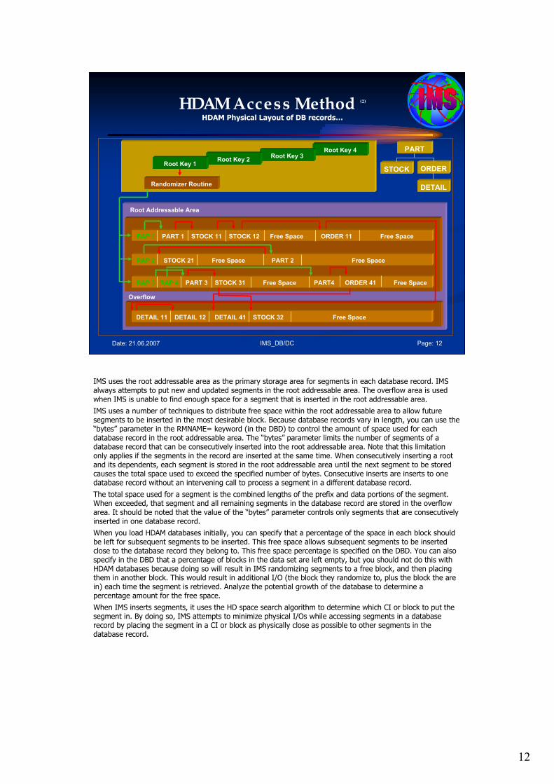
12
IMS_DB/DC Page: 12Date: 21.06.2007
HDAM Access Method (2)
HDAM Physical Layout of DB records…
Randomizer Routine
Root Key 4Root Key 3
Root Key 2Root Key 1
Root Addressable Area
Overflow
RAP 1 PART 1 STOCK 11 STOCK 12 Free Space ORDER 11 Free Space
RAP 2 STOCK 21 Free Space PART 2 Free Space
RAP 3 RAP 4 PART 3 STOCK 31 Free Space PART4 ORDER 41 Free Space
DETAIL 11 DETAIL 12 DETAIL 41 STOCK 32 Free Space
PART
STOCK ORDER
DETAIL
IMS uses the root addressable area as the primary storage area for segments in each database record. IMS always attempts to put new and updated segments in the root addressable area. The overflow area is used when IMS is unable to find enough space for a segment that is inserted in the root addressable area.
IMS uses a number of techniques to distribute free space within the root addressable area to allow future segments to be inserted in the most desirable block. Because database records vary in length, you can use the “bytes” parameter in the RMNAME= keyword (in the DBD) to control the amount of space used for each database record in the root addressable area. The “bytes” parameter limits the number of segments of a database record that can be consecutively inserted into the root addressable area. Note that this limitation only applies if the segments in the record are inserted at the same time. When consecutively inserting a root and its dependents, each segment is stored in the root addressable area until the next segment to be stored causes the total space used to exceed the specified number of bytes. Consecutive inserts are inserts to one database record without an intervening call to process a segment in a different database record.
The total space used for a segment is the combined lengths of the prefix and data portions of the segment. When exceeded, that segment and all remaining segments in the database record are stored in the overflow area. It should be noted that the value of the “bytes” parameter controls only segments that are consecutively inserted in one database record.
When you load HDAM databases initially, you can specify that a percentage of the space in each block should be left for subsequent segments to be inserted. This free space allows subsequent segments to be inserted close to the database record they belong to. This free space percentage is specified on the DBD. You can also specify in the DBD that a percentage of blocks in the data set are left empty, but you should not do this with HDAM databases because doing so will result in IMS randomizing segments to a free block, and then placing them in another block. This would result in additional I/O (the block they randomize to, plus the block the are in) each time the segment is retrieved. Analyze the potential growth of the database to determine a percentage amount for the free space.
When IMS inserts segments, it uses the HD space search algorithm to determine which CI or block to put the segment in. By doing so, IMS attempts to minimize physical I/Os while accessing segments in a database record by placing the segment in a CI or block as physically close as possible to other segments in the database record.
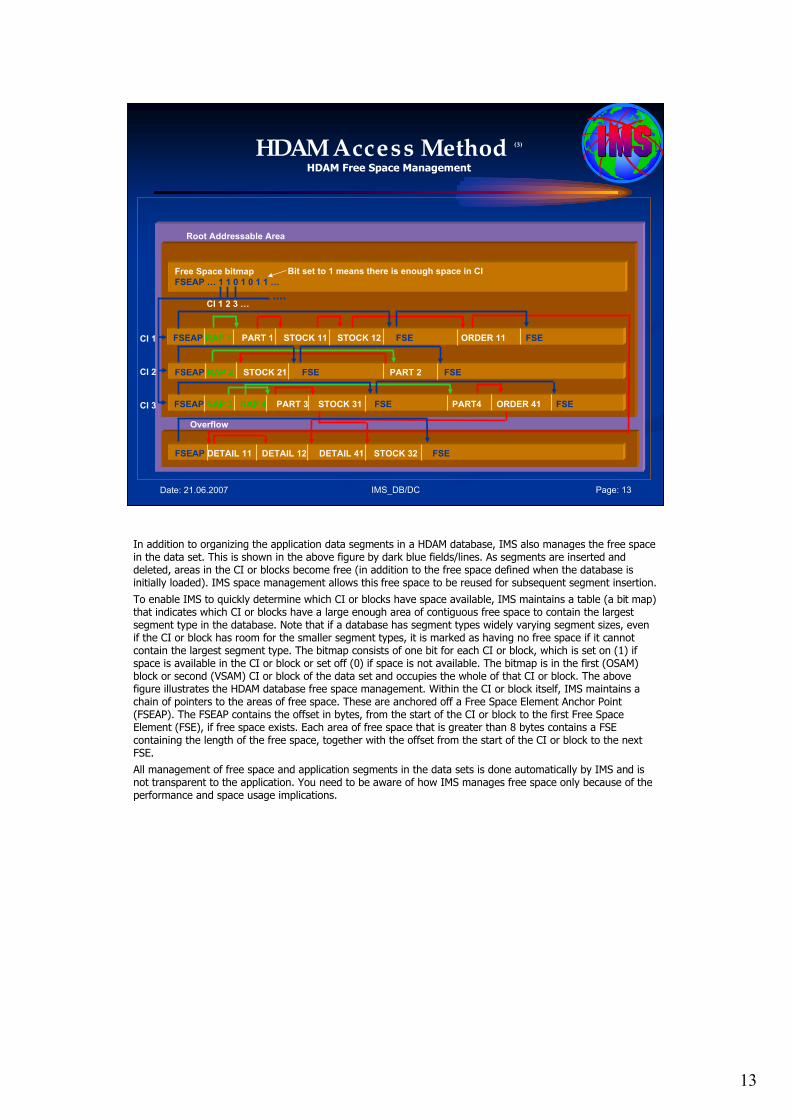
13
IMS_DB/DC Page: 13Date: 21.06.2007
HDAM Access Method (3)
HDAM Free Space Management
Root Addressable Area
Overflow
FSEAP RAP 1 PART 1 STOCK 11 STOCK 12 FSE ORDER 11 FSE
FSEAP RAP 2 STOCK 21 FSE PART 2 FSE
FSEAP RAP 3 RAP 4 PART 3 STOCK 31 FSE PART4 ORDER 41 FSE
FSEAP DETAIL 11 DETAIL 12 DETAIL 41 STOCK 32 FSE
Free Space bitmap
FSEAP … 1 1 0 1 0 1 1 …
Bit set to 1 means there is enough space in CI
CI 1
CI 2
CI 3
CI 1 2 3 …
In addition to organizing the application data segments in a HDAM database, IMS also manages the free space in the data set. This is shown in the above figure by dark blue fields/lines. As segments are inserted and deleted, areas in the CI or blocks become free (in addition to the free space defined when the database is initially loaded). IMS space management allows this free space to be reused for subsequent segment insertion.
To enable IMS to quickly determine which CI or blocks have space available, IMS maintains a table (a bit map) that indicates which CI or blocks have a large enough area of contiguous free space to contain the largest segment type in the database. Note that if a database has segment types widely varying segment sizes, even if the CI or block has room for the smaller segment types, it is marked as having no free space if it cannot contain the largest segment type. The bitmap consists of one bit for each CI or block, which is set on (1) if space is available in the CI or block or set off (0) if space is not available. The bitmap is in the first (OSAM) block or second (VSAM) CI or block of the data set and occupies the whole of that CI or block. The above figure illustrates the HDAM database free space management. Within the CI or block itself, IMS maintains a chain of pointers to the areas of free space. These are anchored off a Free Space Element Anchor Point (FSEAP). The FSEAP contains the offset in bytes, from the start of the CI or block to the first Free Space Element (FSE), if free space exists. Each area of free space that is greater than 8 bytes contains a FSE containing the length of the free space, together with the offset from the start of the CI or block to the next FSE.
All management of free space and application segments in the data sets is done automatically by IMS and is not transparent to the application. You need to be aware of how IMS manages free space only because of the performance and space usage implications.
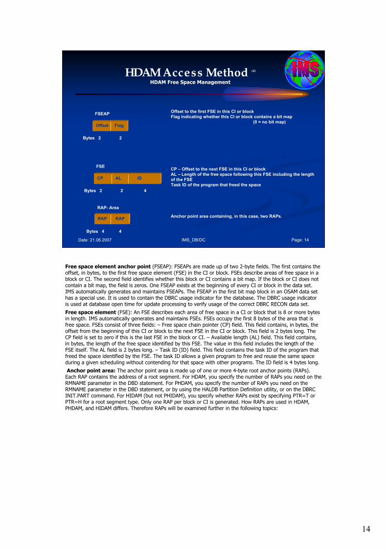
14
IMS_DB/DC Page: 14Date: 21.06.2007
HDAM Access Method (4)
HDAM Free Space Management
Offset Flag
FSEAP
Bytes 2 2
CP AL ID
FSE
Bytes 2 2 4
Offset to the first FSE in this CI or block
Flag indicating whether this CI or block contains a bit map
(0 = no bit map)
CP – Offset to the next FSE in this CI or block
AL – Length of the free space following this FSE including the length
of the FSE
Task ID of the program that freed the space
Anchor point area containing, in this case, two RAPs.RAP RAP
RAP- Area
Bytes 4 4
Free space element anchor point (FSEAP): FSEAPs are made up of two 2-byte fields. The first contains the offset, in bytes, to the first free space element (FSE) in the CI or block. FSEs describe areas of free space in a block or CI. The second field identifies whether this block or CI contains a bit map. If the block or CI does not contain a bit map, the field is zeros. One FSEAP exists at the beginning of every CI or block in the data set. IMS automatically generates and maintains FSEAPs. The FSEAP in the first bit map block in an OSAM data set has a special use. It is used to contain the DBRC usage indicator for the database. The DBRC usage indicator is used at database open time for update processing to verify usage of the correct DBRC RECON data set.
Free space element (FSE): An FSE describes each area of free space in a CI or block that is 8 or more bytes in length. IMS automatically generates and maintains FSEs. FSEs occupy the first 8 bytes of the area that is free space. FSEs consist of three fields: – Free space chain pointer (CP) field. This field contains, in bytes, the offset from the beginning of this CI or block to the next FSE in the CI or block. This field is 2 bytes long. The CP field is set to zero if this is the last FSE in the block or CI. – Available length (AL) field. This field contains, in bytes, the length of the free space identified by this FSE. The value in this field includes the length of the FSE itself. The AL field is 2 bytes long. – Task ID (ID) field. This field contains the task ID of the program that freed the space identified by the FSE. The task ID allows a given program to free and reuse the same space during a given scheduling without contending for that space with other programs. The ID field is 4 bytes long.
Anchor point area: The anchor point area is made up of one or more 4-byte root anchor points (RAPs). Each RAP contains the address of a root segment. For HDAM, you specify the number of RAPs you need on the RMNAME parameter in the DBD statement. For PHDAM, you specify the number of RAPs you need on the RMNAME parameter in the DBD statement, or by using the HALDB Partition Definition utility, or on the DBRC INIT.PART command. For HIDAM (but not PHIDAM), you specify whether RAPs exist by specifying PTR=T or PTR=H for a root segment type. Only one RAP per block or CI is generated. How RAPs are used in HDAM, PHDAM, and HIDAM differs. Therefore RAPs will be examined further in the following topics:
15
IMS_DB/DC Page: 15Date: 21.06.2007
HDAM Access Method (5)
Advantages of the HDAM Access Method:
• fast random access to the root segments,• fast direct access with few I/O operations,• quick access to segments in the DB record,• automatic reuse of space after segment deletions,• can have non-unique root segment keys.
The principle advantages of the HDAM access method are:
•Fast random access to the root segments, via the randomizing routine,
•Fast direct access (no index accesses) with few I/O operations,
•Quick access to segments in a database record, as IMS attempts to store them in the same, or physically near the CI or block,
•Automatic reuse of space after segment deletions,
•Can have non-unique root segment keys.
16
IMS_DB/DC Page: 16Date: 21.06.2007
HDAM Access Method (6)
Disadvantages of the HDAM Access Method:
• cannot access the root segments sequentially in key sequence order,• special actions necessary to load quickly HDAM DBs,• if space exceeds in the root addressable area, it will extend into overflow -> may result into performance problem,• poor performance may be possible if too many keys randomize to the same anchor point.
The principle disadvantages of the HDAM access method are:
•You cannot access the root segments sequentially in key sequence order, unless you create a randomizing module that randomizes into key sequence, or incur the overhead of creating and maintaining a secondary index,
•An HDAM database is slower to load than a HIDAM database, unless you sort the segments into randomizer sequence (for example, by writing user exit routines for the z/OS DFSSORT utility that call the randomizing module or by using the physical sequence sort for Reload utility that is available with the IMS High Performance Load tool from IBM),
•If the database exceeds the space in the root addressable area, it will extend into overflow. After it is in overflow, the performance of the access to these segments can decrease drastically. Note: To increase the space of the database, you must run the DBDGEN utility to increase the number of blocks in the root addressable area and run the ACBGEN utility to rebuild the online ACBs for use in the online system. This will require that you take the database offline (making it unavailable) to complete and coordinate the change,
•Poor performance is possible if too many keys randomize to the same anchor point.
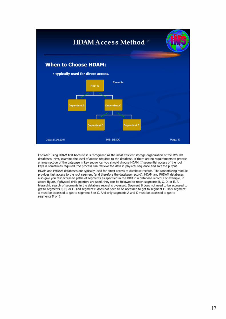
17
IMS_DB/DC Page: 17Date: 21.06.2007
HDAM Access Method (7)
When to Choose HDAM:
• typically used for direct access.
Root A
Dependent B Dependent C
Dependent D Dependent E
Example
Consider using HDAM first because it is recognized as the most efficient storage organization of the IMS HD databases. First, examine the level of access required to the database. If there are no requirements to process a large section of the database in key sequence, you should choose HDAM. If sequential access of the root keys is sometimes required, the process can retrieve the data in physical sequence and sort the putput.
HDAM and PHDAM databases are typically used for direct access to database records. The randomizing module provides fast access to the root segment (and therefore the database record). HDAM and PHDAM databases also give you fast access to paths of segments as specified in the DBD in a database record. For example, in above figure, if physical child pointers are used, they can be followed to reach segments B, C, D, or E. A hierarchic search of segments in the database record is bypassed. Segment B does not need to be accessed to get to segments C, D, or E. And segment D does not need to be accessed to get to segment E. Only segment A must be accessed to get to segment B or C. And only segments A and C must be accessed to get to segments D or E.
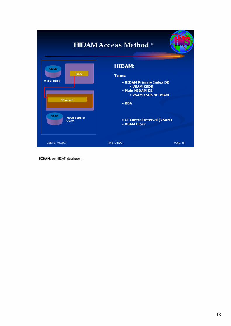
18
IMS_DB/DC Page: 18Date: 21.06.2007
HIDAM Access Method (1)
HIDAM:
Terms:
• HIDAM Primary Index DB• VSAM KSDS
• Main HIDAM DB• VSAM ESDS or OSAM
• RBA
• CI Control Interval (VSAM)• OSAM Block
OS-DSVSAM ESDS or
OSAM
OS-DS
VSAM KSDS
Index
DB record
HIDAM: An HIDAM database …
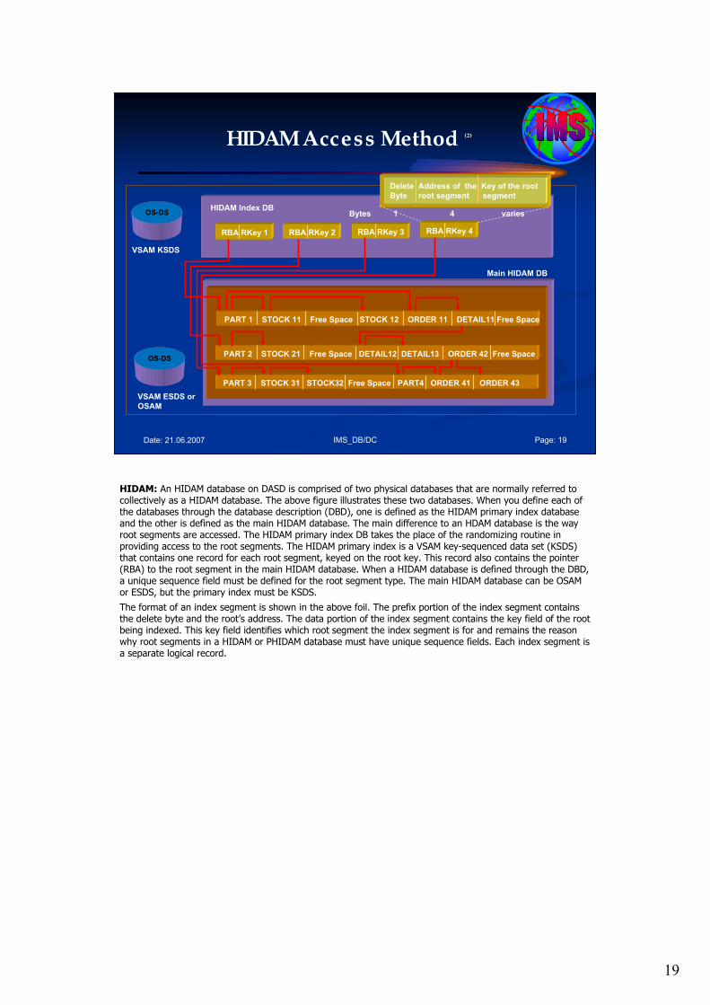
19
IMS_DB/DC Page: 19Date: 21.06.2007
HIDAM Access Method (2)
OS-DS
VSAM ESDS or
OSAM
OS-DS
VSAM KSDS
RBA RKey 1
PART 1 STOCK 11 Free Space STOCK 12 ORDER 11 DETAIL11 Free Space
PART 2 STOCK 21 Free Space DETAIL12 DETAIL13 ORDER 42 Free Space
PART 3 STOCK 31 STOCK32 Free Space PART4 ORDER 41 ORDER 43
RBA RKey 2 RBA RKey 3 RBA RKey 4
HIDAM Index DB
Main HIDAM DB
Bytes 1 4 varies
Delete Address of the Key of the root
Byte root segment segment
HIDAM: An HIDAM database on DASD is comprised of two physical databases that are normally referred to collectively as a HIDAM database. The above figure illustrates these two databases. When you define each of the databases through the database description (DBD), one is defined as the HIDAM primary index database and the other is defined as the main HIDAM database. The main difference to an HDAM database is the way root segments are accessed. The HIDAM primary index DB takes the place of the randomizing routine in providing access to the root segments. The HIDAM primary index is a VSAM key-sequenced data set (KSDS) that contains one record for each root segment, keyed on the root key. This record also contains the pointer (RBA) to the root segment in the main HIDAM database. When a HIDAM database is defined through the DBD, a unique sequence field must be defined for the root segment type. The main HIDAM database can be OSAM or ESDS, but the primary index must be KSDS.
The format of an index segment is shown in the above foil. The prefix portion of the index segment contains the delete byte and the root’s address. The data portion of the index segment contains the key field of the root being indexed. This key field identifies which root segment the index segment is for and remains the reason why root segments in a HIDAM or PHIDAM database must have unique sequence fields. Each index segment is a separate logical record.
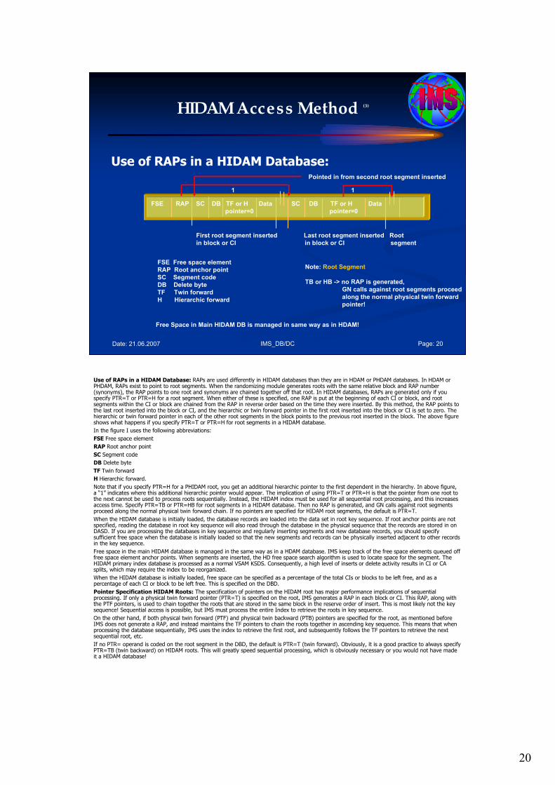
20
IMS_DB/DC Page: 20Date: 21.06.2007
HIDAM Access Method (3)
Use of RAPs in a HIDAM Database:
FSE Free space element
RAP Root anchor point
SC Segment code
DB Delete byte
TF Twin forward
H Hierarchic forward
FSE RAP SC DB TF or H Data SC DB TF or H Data
pointer=0 pointer=0
First root segment inserted Last root segment inserted Root
in block or CI in block or CI segment
Pointed in from second root segment inserted
1 1
Note: Root Segment
TB or HB -> no RAP is generated,
GN calls against root segments proceed
along the normal physical twin forward
pointer!
Free Space in Main HIDAM DB is managed in same way as in HDAM!
Use of RAPs in a HIDAM Database: RAPs are used differently in HIDAM databases than they are in HDAM or PHDAM databases. In HDAM or PHDAM, RAPs exist to point to root segments. When the randomizing module generates roots with the same relative block and RAP number (synonyms), the RAP points to one root and synonyms are chained together off that root. In HIDAM databases, RAPs are generated only if you specify PTR=T or PTR=H for a root segment. When either of these is specified, one RAP is put at the beginning of each CI or block, and root segments within the CI or block are chained from the RAP in reverse order based on the time they were inserted. By this method, the RAP points to the last root inserted into the block or CI, and the hierarchic or twin forward pointer in the first root inserted into the block or CI is set to zero. The hierarchic or twin forward pointer in each of the other root segments in the block points to the previous root inserted in the block. The above figure shows what happens if you specify PTR=T or PTR=H for root segments in a HIDAM database.
In the figure I uses the following abbreviations:
FSE Free space element
RAP Root anchor point
SC Segment code
DB Delete byte
TF Twin forward
H Hierarchic forward.
Note that if you specify PTR=H for a PHIDAM root, you get an additional hierarchic pointer to the first dependent in the hierarchy. In above figure, a “1” indicates where this additional hierarchic pointer would appear. The implication of using PTR=T or PTR=H is that the pointer from one root to the next cannot be used to process roots sequentially. Instead, the HIDAM index must be used for all sequential root processing, and this increases access time. Specify PTR=TB or PTR=HB for root segments in a HIDAM database. Then no RAP is generated, and GN calls against root segments proceed along the normal physical twin forward chain. If no pointers are specified for HIDAM root segments, the default is PTR=T.
When the HIDAM database is initially loaded, the database records are loaded into the data set in root key sequence. If root anchor points are not specified, reading the database in root key sequence will also read through the database in the physical sequence that the records are stored in on DASD. If you are processing the databases in key sequence and regularly inserting segments and new database records, you should specify sufficient free space when the database is initially loaded so that the new segments and records can be physically inserted adjacent to other records in the key sequence.
Free space in the main HIDAM database is managed in the same way as in a HDAM database. IMS keep track of the free space elements queued off free space element anchor points. When segments are inserted, the HD free space search algorithm is used to locate space for the segment. The HIDAM primary index database is processed as a normal VSAM KSDS. Consequently, a high level of inserts or delete activity results in CI or CA splits, which may require the index to be reorganized.
When the HIDAM database is initially loaded, free space can be specified as a percentage of the total CIs or blocks to be left free, and as a percentage of each CI or block to be left free. This is specified on the DBD.
Pointer Specification HIDAM Roots: The specification of pointers on the HIDAM root has major performance implications of sequential processing. If only a physical twin forward pointer (PTR=T) is specified on the root, IMS generates a RAP in each block or CI. This RAP, along with the PTF pointers, is used to chain together the roots that are stored in the same block in the reserve order of insert. This is most likely not the key sequence! Sequential access is possible, but IMS must process the entire Index to retrieve the roots in key sequence.
On the other hand, if both physical twin forward (PTF) and physical twin backward (PTB) pointers are specified for the root, as mentioned before IMS does not generate a RAP, and instead maintains the TF pointers to chain the roots together in ascending key sequence. This means that when processing the database sequentially, IMS uses the index to retrieve the first root, and subsequently follows the TF pointers to retrieve the next sequential root, etc.
If no PTR= operand is coded on the root segment in the DBD, the default is PTR=T (twin forward). Obviously, it is a good practice to always specify PTR=TB (twin backward) on HIDAM roots. This will greatly speed sequential processing, which is obviously necessary or you would not have made it a HIDAM database!
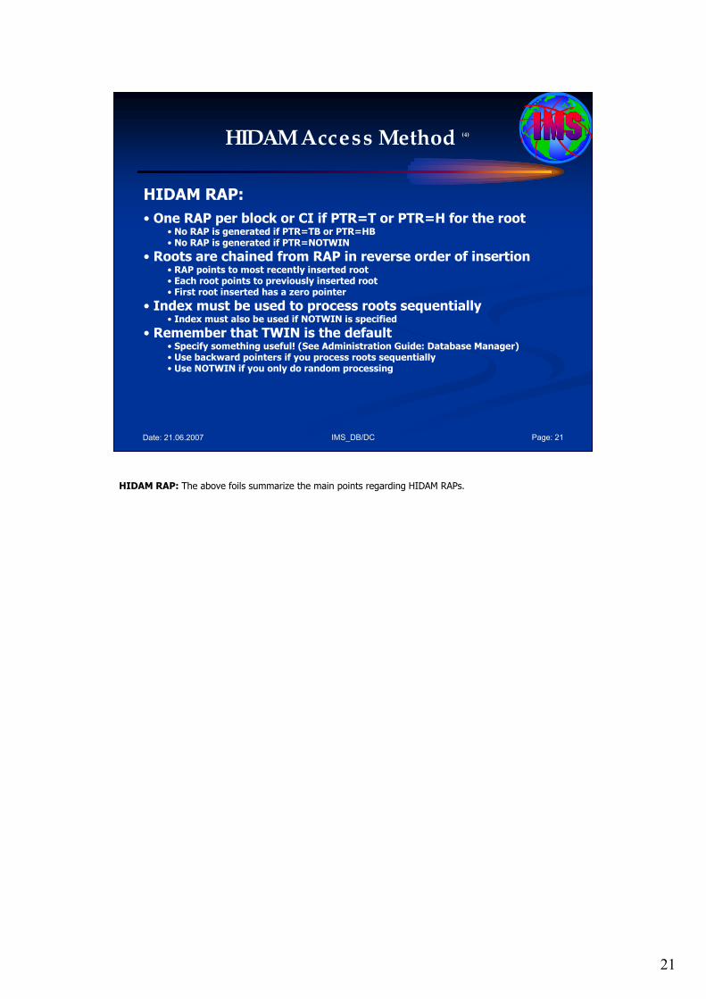
21
IMS_DB/DC Page: 21Date: 21.06.2007
HIDAM Access Method (4)
HIDAM RAP:
• One RAP per block or CI if PTR=T or PTR=H for the root• No RAP is generated if PTR=TB or PTR=HB• No RAP is generated if PTR=NOTWIN
• Roots are chained from RAP in reverse order of insertion• RAP points to most recently inserted root• Each root points to previously inserted root• First root inserted has a zero pointer
• Index must be used to process roots sequentially• Index must also be used if NOTWIN is specified
• Remember that TWIN is the default• Specify something useful! (See Administration Guide: Database Manager)• Use backward pointers if you process roots sequentially• Use NOTWIN if you only do random processing
HIDAM RAP: The above foils summarize the main points regarding HIDAM RAPs.

22
IMS_DB/DC Page: 22Date: 21.06.2007
HIDAM Access Method (5)
Advantages of the HIDAM Access Method:
• The ability to process the root segments and database records in root key sequence,• Quick access to segments in a database record, as IMS attempts to store them in the same, or physically near the, CI or block.• Automatic reuse of space after segment deletions.• The ability to reorganize the HIDAM primary index database in isolation from the main HIDAM database.
The principle advantages of the HIDAM access method are:
•The ability to process the root segments and database records in root key sequence,
•Quick access to segments in a database record, as IMS attempts to store them in the same, or physically near the, CI or block.
•Automatic reuse of space after segment deletions.
•The ability to reorganize the HIDAM primary index database in isolation from the main HIDAM database.
23
IMS_DB/DC Page: 23Date: 21.06.2007
HIDAM Access Method (6)
Disadvantages of the HIDAM Access Method:
• The HIDAM access method has a longer access path, compared to HDAM, when reading root segments randomly by key. There is at least one additional I/O operation to get the HIDAM primary index record before reading the block containing the root segment (excluding any buffering considerations).• Extra DASD space for the HIDAM primary index.• If there is frequent segment insert or delete activity, the HIDAM primary index database requires periodic reorganization to get all database records back to their root key sequence in physical storage.
The principle disadvantages of the HIDAM access method are:
•The HIDAM access method has a longer access path, compared to HDAM, when reading root segments randomly by key. There is at least one additional I/O operation to get the HIDAM primary index record before reading the block containing the root segment (excluding any buffering considerations).
•Extra DASD space for the HIDAM primary index.
•If there is frequent segment insert or delete activity, the HIDAM primary index database requires periodic reorganization to get all database records back to their root key sequence in physical storage.
24
IMS_DB/DC Page: 24Date: 21.06.2007
HIDAM Access Method (7)
When to Choose HIDAM:
•… most common type of database organization,•… need to regularly process the database or part of the database in root segment key sequence.
When to choose HIDAM: HIDAM is the most common type of database organization. HIDAM has the same advantages of the space usage as HDAM, but also keeps the root keys available in sequence. These days, with the speed of DASD, the extra read of the primary index database can be incurred without much overhead by specifying specific buffer pools for the primary index database to use, thus reducing the actual I/O to use the index pointer segments.
Choose HIDAM only if you need to regularly process the database in root segment key sequence. If you also need fast random access to roots from online systems, look at alternatives for the sequential access, such as unload and sort or secondary indexes.
HIDAM does not need to be monitored as closely as HDAM…

25
IMS_DB/DC Page: 25Date: 21.06.2007
HD Access Methods
Recommendations for using HD Access Methods:
1. Database records have great variations in their sizes,2. Database records are large and contain many types of segments,3. There are high volumes of deletes and inserts in the database,4. The database may have significant growth.
Recommendations for using HD Access Methods:
1. Database records have great variations in their sizes,
2. Database records are large and contain many types of segments,
3. There are high volumes of deletes and inserts in the database,
4. The database may have significant growth.

26
IMS_DB/DC Page: 26Date: 21.06.2007
Agenda Session 3: Hierarchical Access Methods
1. HD Databases• HDAM & HIDAM Access Method
• PHDAM & PHIDAM Access Methods
2. Index Databases
3. Fast Path DEDBs
4. GSAM Access Method
5. HS Databases
• HSAM & HISAM Access Method
6. Operating System Access Methods
7. Data Set Groups
8. Summary
PHDAM& PHIDAM Access Method.
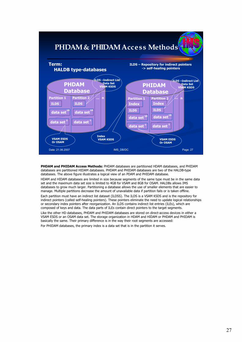
27
IMS_DB/DC Page: 27Date: 21.06.2007
PHDAM & PHIDAM Access Methods (1)
Term: HALDB type-databases
ILDS – Repository for indirect pointers-> self-healing pointers
PHDAMDatabase
data set1
data set10
ILDS
Partition 1
data set1
data set10
ILDS
Partition 2 n…
ILDS –Indirect ListData Set
VSAM KSDS PHIDAMDatabase
data set1
data set10
ILDS
Partition 1
data set1
data set10
ILDS
Partition 2 n…
Index Index
ILDS –Indirect ListData Set
VSAM KSDS
IndexVSAM KSDSVSAM ESDS
Or OSAMVSAM ESDSOr OSAM
PHDAM and PHIDAM Access Methods: PHDAM databases are partitioned HDAM databases, and PHIDAM databases are partitioned HIDAM databases. PHDAM and PHIDAM databases are two of the HALDB-type databases. The above figure illustrates a logical view of an PDAM and PHIDAM database.
HDAM and HIDAM databases are limited in size because segments of the same type must be in the same data set and the maximum data set size is limited to 4GB for VSAM and 8GB for OSAM. HALDBs allows IMS databases to grow much larger. Partitioning a database allows the use of smaller elements that are easier to manage. Multiple partitions decrease the amount of unavailable data if partition fails or is taken offline.
Each partition must have an indirect list dataset (ILDSS). The ILDS is a VSAM KSDS and is the repository for indirect pointers (called self-healing pointers). These pointers eliminate the need to update logical relationships or secondary index pointers after reorganization. An ILDS contains indirect list entries (ILEs), which are composed of keys and data. The data parts of ILEs contain direct pointers to the target segments.
Like the other HD databases, PHDAM and PHIDAM databases are stored on direct-access devices in either a VSAM ESDS or an OSAM data set. The storage organization in HDAM and HIDAM or PHDAM and PHIDAM is basically the same. Their primary difference is in the way their root segments are accessed:
For PHIDAM databases, the primary index is a data set that is in the partition it serves.
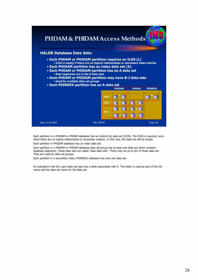
28
IMS_DB/DC Page: 28Date: 21.06.2007
PHDAM & PHIDAM Access Methods (1)
HALDB Database Data Sets:
• Each PHDAM or PHIDAM partition requires an ILDS (L)• ILDS is empty if there are no logical relationships or secondary index entries
• Each PHIDAM partition has an index data set (X)• Each PHDAM or PHIDAM partition has an A data set
• Root segments are in the A data sets
• Each PHDAM or PHIDAM partition may have B-J data sets• Used for multiple data set groups
• Each PSINDEX partition has an A data setPHIDAM PHDAM PSINDEX
Index
ILDS
Data
X…
L…
A…
J
A…
J
L…
A…
Each partition in a PHIDAM or PHDAM database has an indirect list data set (ILDS). The ILDS is required, even when there are no logical relationships or secondary indexes. In this case, the data set will be empty.
Each partition in PHIDAM database has an index data set.
Each partition in a PHIDAM or PHDAM database data set group has at least one data set which contains database segments. These data sets are called “data data sets”. There may be up to ten of these data set. They are used for data set groups.
Each partition in a secondary index (PSINDEX) database has only one data set.
As indicated in the foil, each data set type has a letter associated with it. This letter is used as part of the DD name and the data set name for the data set.
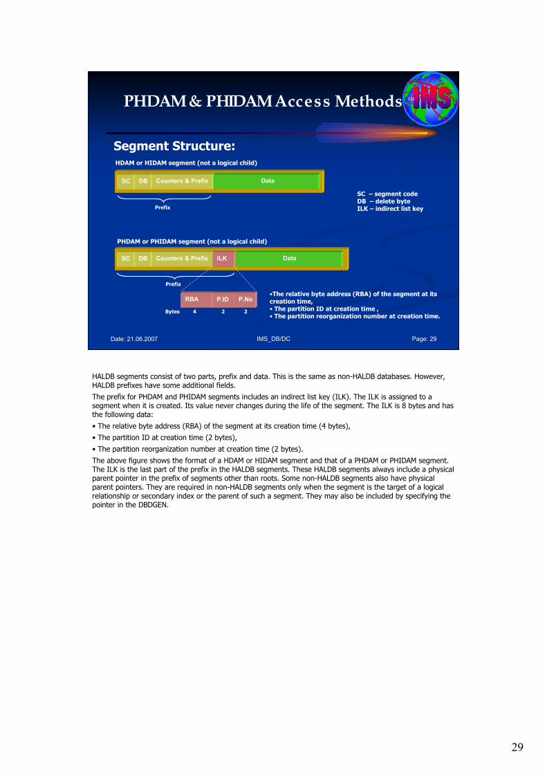
29
IMS_DB/DC Page: 29Date: 21.06.2007
PHDAM & PHIDAM Access Methods (2)
Segment Structure:
SC – segment codeDB – delete byteILK – indirect list key
SC DB Counters & Prefix Data
HDAM or HIDAM segment (not a logical child)
Prefix
•The relative byte address (RBA) of the segment at its creation time,• The partition ID at creation time ,• The partition reorganization number at creation time.
SC DB Counters & Prefix DataILK
PHDAM or PHIDAM segment (not a logical child)
Prefix
RBA P.ID P.No
Bytes 4 2 2
HALDB segments consist of two parts, prefix and data. This is the same as non-HALDB databases. However, HALDB prefixes have some additional fields.
The prefix for PHDAM and PHIDAM segments includes an indirect list key (ILK). The ILK is assigned to a segment when it is created. Its value never changes during the life of the segment. The ILK is 8 bytes and has the following data:
• The relative byte address (RBA) of the segment at its creation time (4 bytes),
• The partition ID at creation time (2 bytes),
• The partition reorganization number at creation time (2 bytes).
The above figure shows the format of a HDAM or HIDAM segment and that of a PHDAM or PHIDAM segment. The ILK is the last part of the prefix in the HALDB segments. These HALDB segments always include a physical parent pointer in the prefix of segments other than roots. Some non-HALDB segments also have physical parent pointers. They are required in non-HALDB segments only when the segment is the target of a logical relationship or secondary index or the parent of such a segment. They may also be included by specifying the pointer in the DBDGEN.
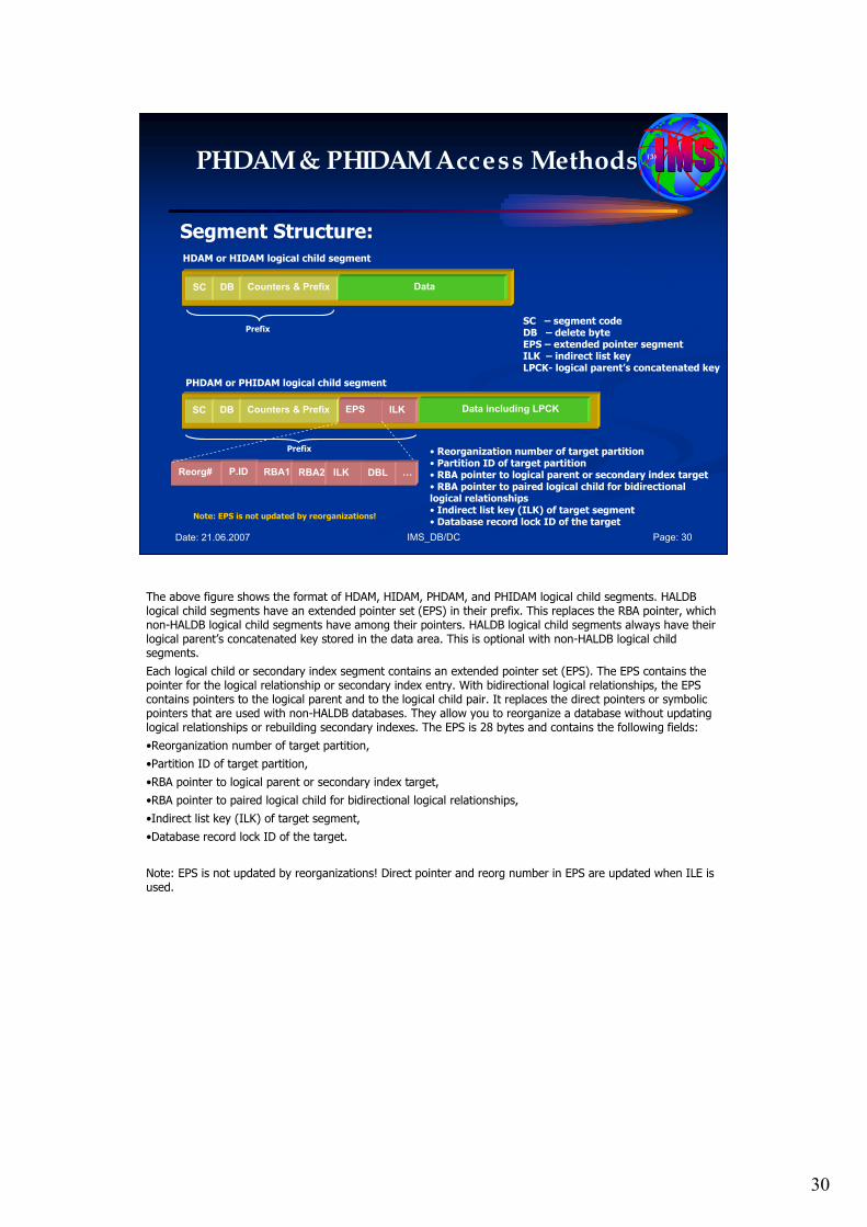
30
IMS_DB/DC Page: 30Date: 21.06.2007
PHDAM & PHIDAM Access Methods (3)
Segment Structure:
SC – segment codeDB – delete byteEPS – extended pointer segmentILK – indirect list keyLPCK- logical parent’s concatenated key
SC DB Counters & Prefix Data
HDAM or HIDAM logical child segment
Prefix
• Reorganization number of target partition• Partition ID of target partition• RBA pointer to logical parent or secondary index target• RBA pointer to paired logical child for bidirectional logical relationships• Indirect list key (ILK) of target segment• Database record lock ID of the target
Prefix
SC DB Counters & Prefix
PHDAM or PHIDAM logical child segment
EPS ILK Data including LPCK
Note: EPS is not updated by reorganizations!
Reorg# P.ID RBA1 RBA2 ILK DBL …
The above figure shows the format of HDAM, HIDAM, PHDAM, and PHIDAM logical child segments. HALDB logical child segments have an extended pointer set (EPS) in their prefix. This replaces the RBA pointer, which non-HALDB logical child segments have among their pointers. HALDB logical child segments always have their logical parent’s concatenated key stored in the data area. This is optional with non-HALDB logical child segments.
Each logical child or secondary index segment contains an extended pointer set (EPS). The EPS contains the pointer for the logical relationship or secondary index entry. With bidirectional logical relationships, the EPS contains pointers to the logical parent and to the logical child pair. It replaces the direct pointers or symbolic pointers that are used with non-HALDB databases. They allow you to reorganize a database without updating logical relationships or rebuilding secondary indexes. The EPS is 28 bytes and contains the following fields:
•Reorganization number of target partition,
•Partition ID of target partition,
•RBA pointer to logical parent or secondary index target,
•RBA pointer to paired logical child for bidirectional logical relationships,
•Indirect list key (ILK) of target segment,
•Database record lock ID of the target.
Note: EPS is not updated by reorganizations! Direct pointer and reorg number in EPS are updated when ILE is used.

31
IMS_DB/DC Page: 31Date: 21.06.2007
PHDAM & PHIDAM Access Methods (4)
Self Healing Pointers
Segments are uniquely identified by an ILK (Indirect List Key)
• ILK• Uniquely identifies a segment (8 bytes)• RBA of segment at its creation time (4 bytes)• Partition id at creation time (2 bytes)
• Reorg number at creation time (2 bytes)• Created when INSERTed into the database• Application program• HD Reload with MIGRATE=YES used in HD unloadedfrom non-HALDB database– Kept unchanged until segment is deleted
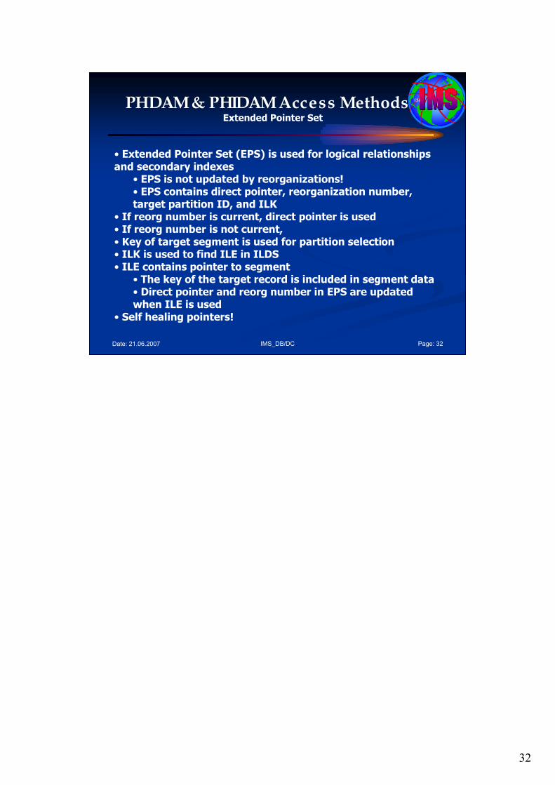
32
IMS_DB/DC Page: 32Date: 21.06.2007
PHDAM & PHIDAM Access Methods (5)
Extended Pointer Set
• Extended Pointer Set (EPS) is used for logical relationships and secondary indexes
• EPS is not updated by reorganizations!• EPS contains direct pointer, reorganization number, target partition ID, and ILK
• If reorg number is current, direct pointer is used• If reorg number is not current,• Key of target segment is used for partition selection• ILK is used to find ILE in ILDS• ILE contains pointer to segment
• The key of the target record is included in segment data• Direct pointer and reorg number in EPS are updated when ILE is used
• Self healing pointers!
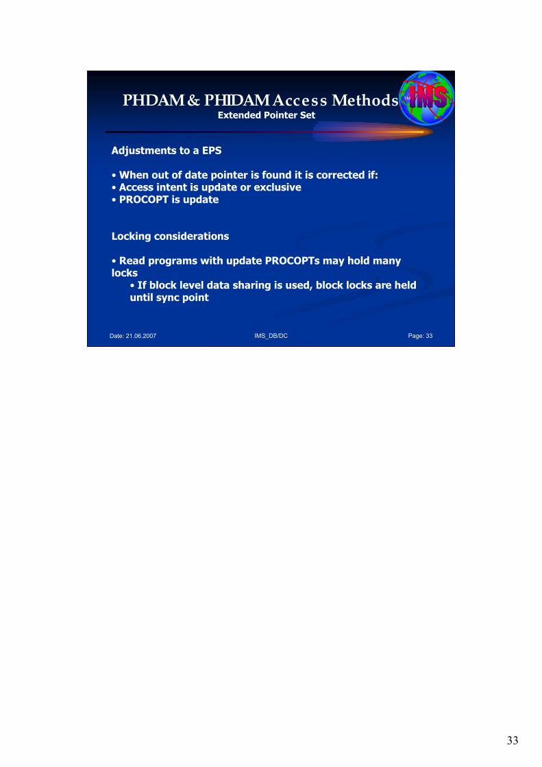
33
IMS_DB/DC Page: 33Date: 21.06.2007
PHDAM & PHIDAM Access Methods (6)
Extended Pointer Set
Adjustments to a EPS
•When out of date pointer is found it is corrected if:• Access intent is update or exclusive• PROCOPT is update
Locking considerations
• Read programs with update PROCOPTs may hold manylocks
• If block level data sharing is used, block locks are held until sync point
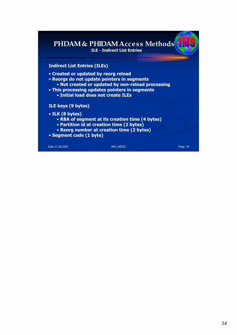
34
IMS_DB/DC Page: 34Date: 21.06.2007
PHDAM & PHIDAM Access Methods (7)
ILE - Indirect List Entries
Indirect List Entries (ILEs)
• Created or updated by reorg reload• Reorgs do not update pointers in segments
• Not created or updated by non-reload processing• This processing updates pointers in segments
• Initial load does not create ILEs
ILE keys (9 bytes)
• ILK (8 bytes)• RBA of segment at its creation time (4 bytes)• Partition id at creation time (2 bytes)• Reorg number at creation time (2 bytes)
• Segment code (1 byte)
35
IMS_DB/DC Page: 35Date: 21.06.2007
PHDAM & PHIDAM Access Methods (8)
When to choose PHDAM or PHIDAM:
• same as for choosing HDAM and HIDAM…
• the differences are the size of the data store and some administrative considerations.
•Note: Exceptions!
Related Reading: For more information about HALDBs, see IMS Administration Guide: Database Manager and the IBM Redbook: The Complete IMS HALDB Guide All You Need to Know to Manage HALDBs.
When to choose PHDAM or PHIDAM: The reasons for choosing PHDAM or PHIDAM are the same as described before for HDAM or HIDAM. The differences are the size of the data store and some administrative considerations.
You might not need to change any of your application programs when you migrate HDAM or HIDAM databases to HALDBs, but there might be exceptions. Exceptions include the initial loading of logically related databases and the processing of secondary indexes as databases.
You might also want to change applications to take advantage of some HALDB capabilities. These capabilities include processing in parallel, processing individual partitions, and handling unavailable partitions.

36
IMS_DB/DC Page: 36Date: 21.06.2007
(P)HDAM vs (P)HIDAM
Recommendations Summary for (P)HDAM vs. (P)HIDAM:
• PHIDAM and HIDAM have the following advantages over PHDAM and HDAM:
1. They tend to use less space.2. They allow you easily to process a DB in root key sequence.
• PHDAM and HDAM have the following advantages over PHIDAM and HIDAM:
1. They tend to require fewer I/Os to retrieve and insert root segments,
2. They tend to require fewer organizations when update activity is concentrated in a range of keys,
3. They tend to handle space management with creeping root keys better.
Recommendations Summary for (P)HDAM vs. (P)HIDAM:
• PHIDAM and HIDAM have the following advantages over PHDAM and HDAM:
1. They tend to use less space. This provides a performance advantage for batch jobs which sequentially process the entire database.
2. They allow you easily to process a DB in root key sequence.
PHDAM and HDAM have the following advantages over PHIDAM and HIDAM:
1. They tend to require fewer I/Os to retrieve and insert root segments,
2. They tend to require fewer organizations when update activity is concentrated in a range of keys,
3. They tend to handle space management with creeping root keys better.

37
IMS_DB/DC Page: 37Date: 21.06.2007
Agenda Session 3: Hierarchical Access Methods
1. HD Databases
• HDAM & HIDAM Access Method
• PHDAM & PHIDAM Access Methods
2. Index Databases
3. Fast Path DEDBs
4. GSAM Access Method
5. HS Databases
• HSAM & HISAM Access Method
6. Operating System Access Methods
7. Data Set Groups
8. Summary
2. Index Databases.

38
IMS_DB/DC Page: 38Date: 21.06.2007
Index Databases (1)
Types:
• Primary Index of HIDAM and PHIDAM databases,
• Index databases
• partitioned secondary Index databases (PSINDEX)
• VSAM KSDS• associated with another HD database
• Secondary Index: pointer RBA or symbolic• HIDAM primary Index: pointer always direct
Index databases are used to implement secondary indexes and the primary index of HIDAM and PHIDAM databases. An index database is always associated with another HD database and cannot exist by itself. An index database can, however, be processed separately by an application program.
An index database consists of a single VSAM KSDS. Unlike the VSAM ESDSs used by IMS, which are processed at the block or control interval level, the index database is processed as a normal indexed file. IMS uses the normal VSAM access method macros to process it.
The records in the KSDS contain the fields that make up the key, and a pointer to the target segment. For a secondary index, the pointer can be direct (relative byte address of the target segment) or symbolic (the complete, concatenated key of the target segment). For a HIDAM primary index, the pointer is always direct.
Another type of HALDB is a partitioned secondary index (PSINDEX) database. A PSINDEX database is the partitioned version of the HD secondary index database discussed earlier. All the concepts that apply to the HD secondary index databases apply to PSINDEX databases. The only real difference is that PSINDEX pointer segments can point only to target segments that reside in HALDBs.
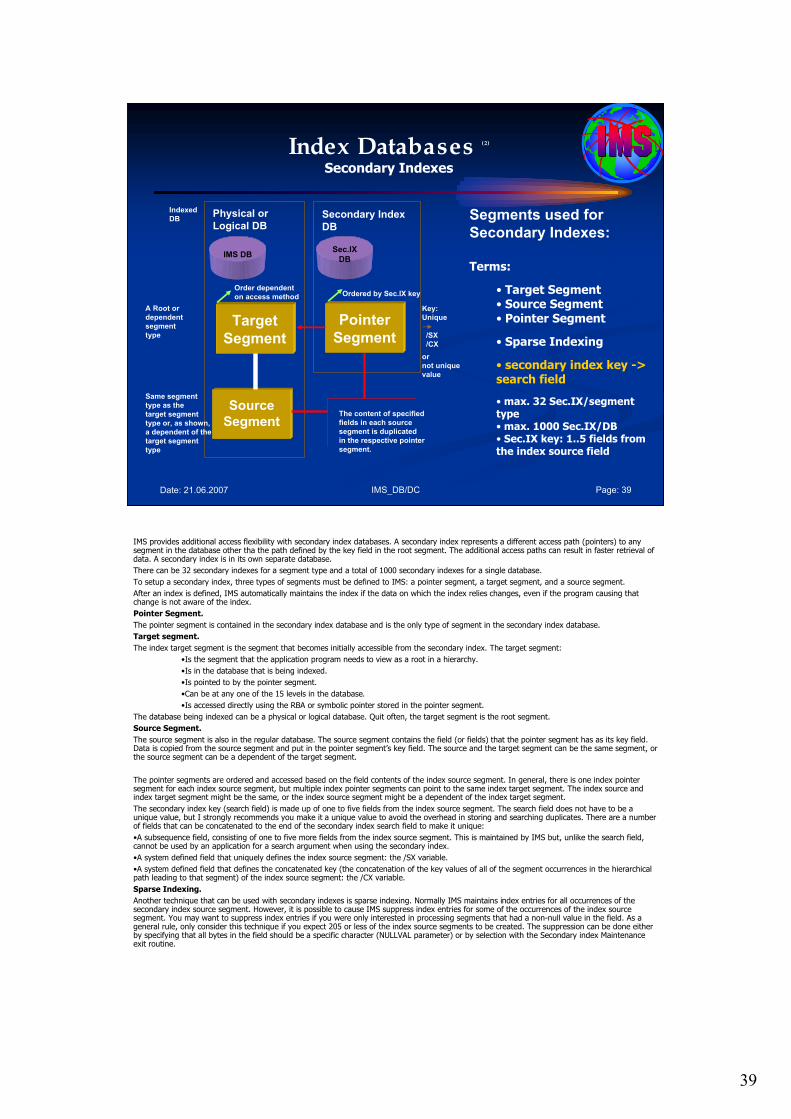
39
IMS_DB/DC Page: 39Date: 21.06.2007
Index Databases (2)
Secondary Indexes
Segments used for
Secondary Indexes:
Terms:
• Target Segment• Source Segment• Pointer Segment
• Sparse Indexing
• secondary index key -> search field
• max. 32 Sec.IX/segment type• max. 1000 Sec.IX/DB• Sec.IX key: 1..5 fields from the index source field
Pointer
Segment
Secondary Index
DB
Sec.IX
DB
Ordered by Sec.IX key
Key:
Unique
/SX
/CX
or
not unique
value
Target
Segment
Source
Segment
A Root or
dependent
segment
type
Same segment
type as the
target segment
type or, as shown,
a dependent of the
target segment
type
Physical or
Logical DB
IMS DB
Order dependent
on access method
Indexed
DB
The content of specified
fields in each source
segment is duplicated
in the respective pointer
segment.
IMS provides additional access flexibility with secondary index databases. A secondary index represents a different access path (pointers) to any segment in the database other tha the path defined by the key field in the root segment. The additional access paths can result in faster retrieval of data. A secondary index is in its own separate database.
There can be 32 secondary indexes for a segment type and a total of 1000 secondary indexes for a single database.
To setup a secondary index, three types of segments must be defined to IMS: a pointer segment, a target segment, and a source segment.
After an index is defined, IMS automatically maintains the index if the data on which the index relies changes, even if the program causing that change is not aware of the index.
Pointer Segment.
The pointer segment is contained in the secondary index database and is the only type of segment in the secondary index database.
Target segment.
The index target segment is the segment that becomes initially accessible from the secondary index. The target segment:
•Is the segment that the application program needs to view as a root in a hierarchy.
•Is in the database that is being indexed.
•Is pointed to by the pointer segment.
•Can be at any one of the 15 levels in the database.
•Is accessed directly using the RBA or symbolic pointer stored in the pointer segment.
The database being indexed can be a physical or logical database. Quit often, the target segment is the root segment.
Source Segment.
The source segment is also in the regular database. The source segment contains the field (or fields) that the pointer segment has as its key field. Data is copied from the source segment and put in the pointer segment’s key field. The source and the target segment can be the same segment, or the source segment can be a dependent of the target segment.
The pointer segments are ordered and accessed based on the field contents of the index source segment. In general, there is one index pointer segment for each index source segment, but multiple index pointer segments can point to the same index target segment. The index source and index target segment might be the same, or the index source segment might be a dependent of the index target segment.
The secondary index key (search field) is made up of one to five fields from the index source segment. The search field does not have to be a unique value, but I strongly recommends you make it a unique value to avoid the overhead in storing and searching duplicates. There are a number of fields that can be concatenated to the end of the secondary index search field to make it unique:
•A subsequence field, consisting of one to five more fields from the index source segment. This is maintained by IMS but, unlike the search field, cannot be used by an application for a search argument when using the secondary index.
•A system defined field that uniquely defines the index source segment: the /SX variable.
•A system defined field that defines the concatenated key (the concatenation of the key values of all of the segment occurrences in the hierarchical path leading to that segment) of the index source segment: the /CX variable.
Sparse Indexing.
Another technique that can be used with secondary indexes is sparse indexing. Normally IMS maintains index entries for all occurrences of the secondary index source segment. However, it is possible to cause IMS suppress index entries for some of the occurrences of the index source segment. You may want to suppress index entries if you were only interested in processing segments that had a non-null value in the field. As a general rule, only consider this technique if you expect 205 or less of the index source segments to be created. The suppression can be done either by specifying that all bytes in the field should be a specific character (NULLVAL parameter) or by selection with the Secondary index Maintenance exit routine.
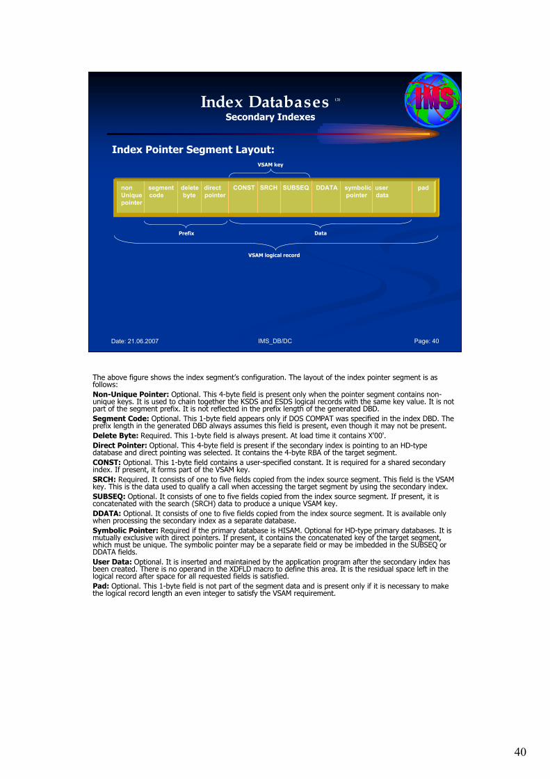
40
IMS_DB/DC Page: 40Date: 21.06.2007
Index Databases (3)
Secondary Indexes
Index Pointer Segment Layout:
non segment delete direct CONST SRCH SUBSEQ DDATA symbolic user pad
Unique code byte pointer pointer data
pointer
VSAM key
Prefix Data
VSAM logical record
The above figure shows the index segment’s configuration. The layout of the index pointer segment is as follows:
Non-Unique Pointer: Optional. This 4-byte field is present only when the pointer segment contains non-unique keys. It is used to chain together the KSDS and ESDS logical records with the same key value. It is not part of the segment prefix. It is not reflected in the prefix length of the generated DBD.
Segment Code: Optional. This 1-byte field appears only if DOS COMPAT was specified in the index DBD. The prefix length in the generated DBD always assumes this field is present, even though it may not be present.
Delete Byte: Required. This 1-byte field is always present. At load time it contains X'00'.
Direct Pointer: Optional. This 4-byte field is present if the secondary index is pointing to an HD-type database and direct pointing was selected. It contains the 4-byte RBA of the target segment.
CONST: Optional. This 1-byte field contains a user-specified constant. It is required for a shared secondary index. If present, it forms part of the VSAM key.
SRCH: Required. It consists of one to five fields copied from the index source segment. This field is the VSAM key. This is the data used to qualify a call when accessing the target segment by using the secondary index.
SUBSEQ: Optional. It consists of one to five fields copied from the index source segment. If present, it is concatenated with the search (SRCH) data to produce a unique VSAM key.
DDATA: Optional. It consists of one to five fields copied from the index source segment. It is available only when processing the secondary index as a separate database.
Symbolic Pointer: Required if the primary database is HISAM. Optional for HD-type primary databases. It is mutually exclusive with direct pointers. If present, it contains the concatenated key of the target segment, which must be unique. The symbolic pointer may be a separate field or may be imbedded in the SUBSEQ or DDATA fields.
User Data: Optional. It is inserted and maintained by the application program after the secondary index has been created. There is no operand in the XDFLD macro to define this area. It is the residual space left in the logical record after space for all requested fields is satisfied.
Pad: Optional. This 1-byte field is not part of the segment data and is present only if it is necessary to make the logical record length an even integer to satisfy the VSAM requirement.
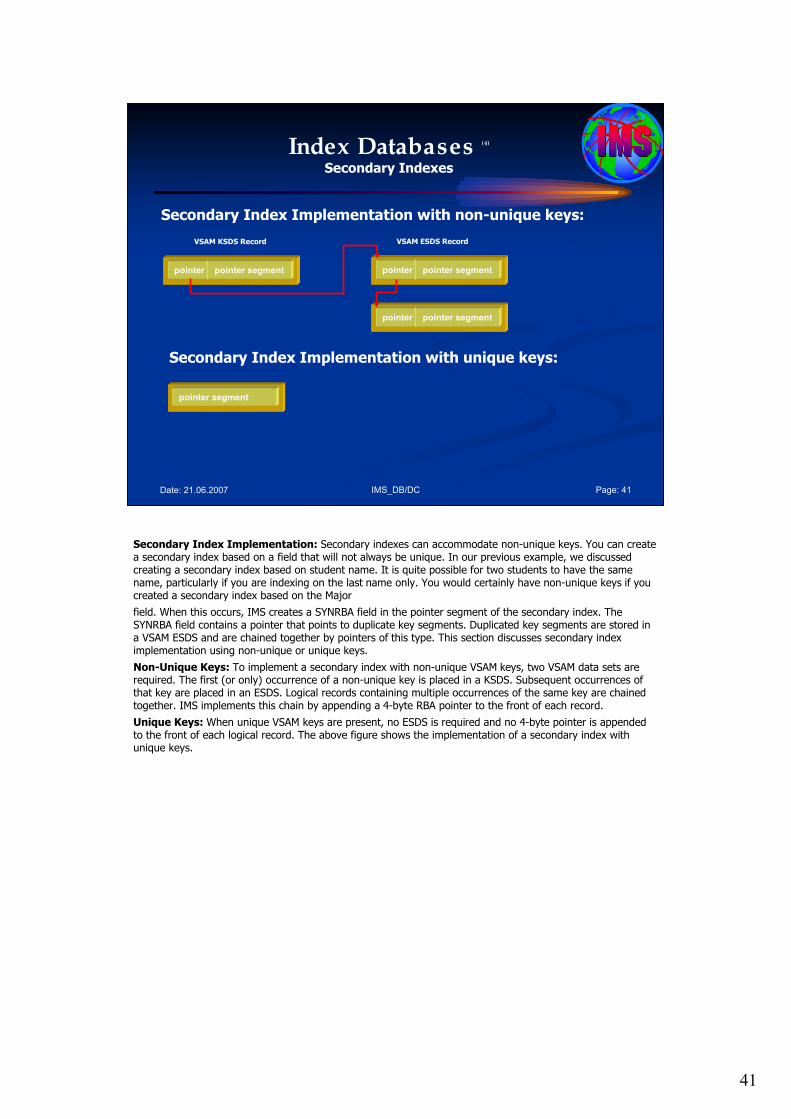
41
IMS_DB/DC Page: 41Date: 21.06.2007
Index Databases (4)
Secondary Indexes
Secondary Index Implementation with non-unique keys:
pointer pointer segment
VSAM KSDS Record
pointer pointer segment
pointer pointer segment
VSAM ESDS Record
pointer segment
Secondary Index Implementation with unique keys:
Secondary Index Implementation: Secondary indexes can accommodate non-unique keys. You can create a secondary index based on a field that will not always be unique. In our previous example, we discussed creating a secondary index based on student name. It is quite possible for two students to have the same name, particularly if you are indexing on the last name only. You would certainly have non-unique keys if you created a secondary index based on the Major
field. When this occurs, IMS creates a SYNRBA field in the pointer segment of the secondary index. The SYNRBA field contains a pointer that points to duplicate key segments. Duplicated key segments are stored in a VSAM ESDS and are chained together by pointers of this type. This section discusses secondary index implementation using non-unique or unique keys.
Non-Unique Keys: To implement a secondary index with non-unique VSAM keys, two VSAM data sets are required. The first (or only) occurrence of a non-unique key is placed in a KSDS. Subsequent occurrences of that key are placed in an ESDS. Logical records containing multiple occurrences of the same key are chained together. IMS implements this chain by appending a 4-byte RBA pointer to the front of each record.
Unique Keys: When unique VSAM keys are present, no ESDS is required and no 4-byte pointer is appended to the front of each logical record. The above figure shows the implementation of a secondary index with unique keys.
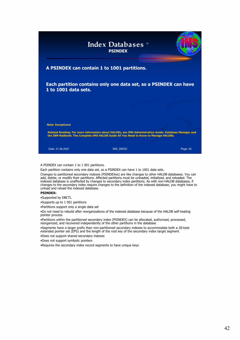
42
IMS_DB/DC Page: 42Date: 21.06.2007
Index Databases (5)
PSINDEX
A PSINDEX can contain 1 to 1001 partitions.
Each partition contains only one data set, so a PSINDEX can have1 to 1001 data sets.
Note: Exceptions!
Related Reading: For more information about HALDBs, see IMS Administration Guide: Database Manager and the IBM Redbook: The Complete IMS HALDB Guide All You Need to Know to Manage HALDBs.
A PSINDEX can contain 1 to 1 001 partitions.
Each partition contains only one data set, so a PSINDEX can have 1 to 1001 data sets.
Changes to partitioned secondary indexes (PSINDEXes) are like changes to other HALDB databases. You can add, delete, or modify their partitions. Affected partitions must be unloaded, initialized, and reloaded. The indexed database is unaffected by changes to secondary index partitions. As with non-HALDB databases, if changes to the secondary index require changes to the definition of the indexed database, you might have to unload and reload the indexed database.
PSINDEX:
•Supported by DBCTL
•Supports up to 1 001 partitions
•Partitions support only a single data set
•Do not need to rebuild after reorganizations of the indexed database because of the HALDB self-healing pointer process
•Partitions within the partitioned secondary index (PSINDEX) can be allocated, authorized, processed, reorganized, and recovered independently of the other partitions in the database
•Segments have a larger prefix than non-partitioned secondary indexes to accommodate both a 28-byte extended pointer set (EPS) and the length of the root key of the secondary index target segment
•Does not support shared secondary indexes
•Does not support symbolic pointers
•Requires the secondary index record segments to have unique keys
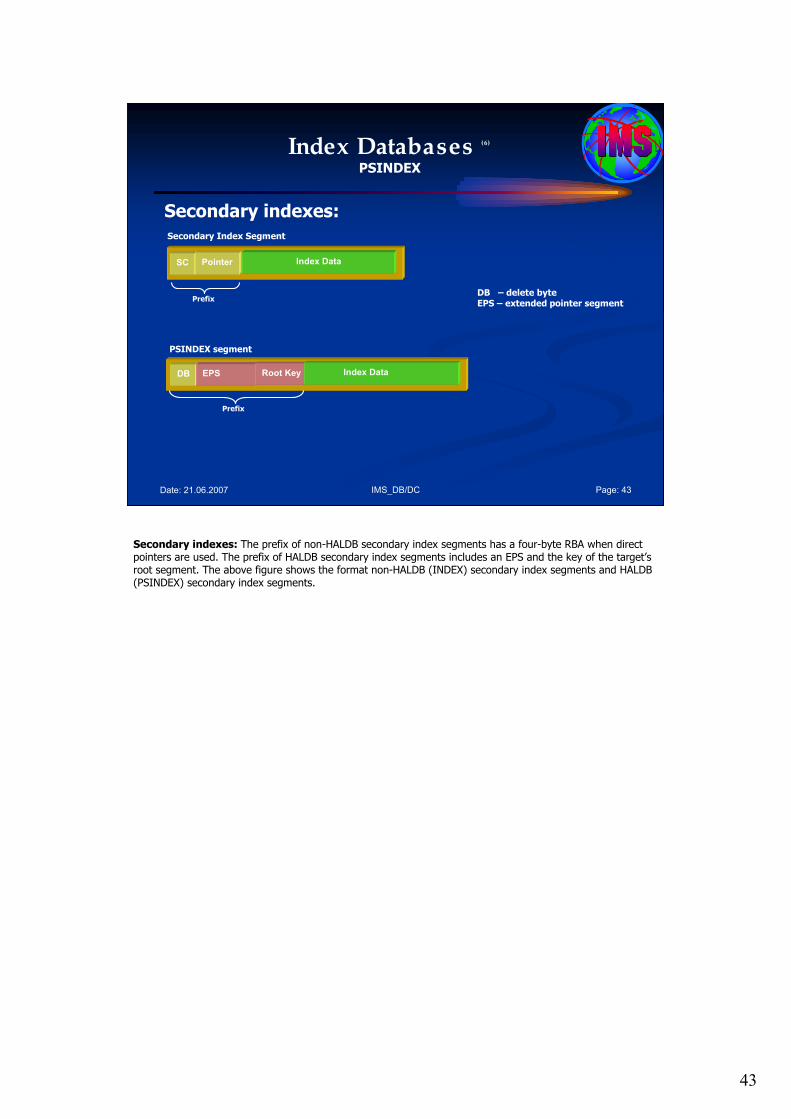
43
IMS_DB/DC Page: 43Date: 21.06.2007
Index Databases (6)
PSINDEX
Secondary indexes:
DB – delete byteEPS – extended pointer segment
SC Pointer Index Data
Secondary Index Segment
Prefix
DB
PSINDEX segment
Prefix
EPS Root Key Index Data
Secondary indexes: The prefix of non-HALDB secondary index segments has a four-byte RBA when direct pointers are used. The prefix of HALDB secondary index segments includes an EPS and the key of the target’s root segment. The above figure shows the format non-HALDB (INDEX) secondary index segments and HALDB (PSINDEX) secondary index segments.
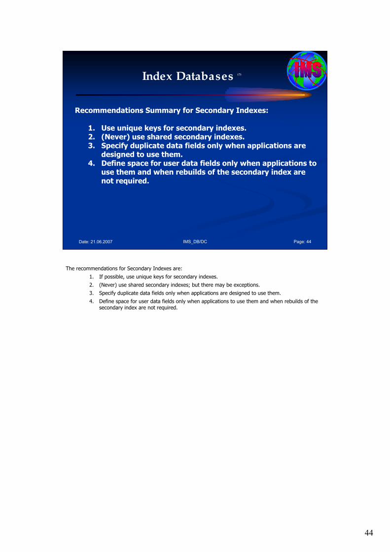
44
IMS_DB/DC Page: 44Date: 21.06.2007
Index Databases (7)
Recommendations Summary for Secondary Indexes:
1. Use unique keys for secondary indexes.2. (Never) use shared secondary indexes.3. Specify duplicate data fields only when applications are
designed to use them.4. Define space for user data fields only when applications to
use them and when rebuilds of the secondary index are not required.
The recommendations for Secondary Indexes are:
1. If possible, use unique keys for secondary indexes.
2. (Never) use shared secondary indexes; but there may be exceptions.
3. Specify duplicate data fields only when applications are designed to use them.
4. Define space for user data fields only when applications to use them and when rebuilds of the secondary index are not required.
45
IMS_DB/DC Page: 45Date: 21.06.2007
Agenda Session 3: Hierarchical Access Methods
1. HD Databases
• HDAM & HIDAM Access Method
• PHDAM & PHIDAM Access Methods
2. Index Databases
3. Fast Path DEDBs
4. GSAM Access Method
5. HS Databases
• HSAM & HISAM Access Method
6. Operating System Access Methods
7. Data Set Groups
8. Summary
3. Fast Path DEDBs.
46
IMS_DB/DC Page: 46Date: 21.06.2007
Fast Path DEDBs (1)
Fast Path DEDBs:
-> broadly same as HDAM access method,
However there are important differences:
• To provide the additional features offered by DEDBs, the implementation of the DEDB access method onto operating system access method data sets is different (and significantly more complicated) than with HDAM,
• There are restrictions on the facilities available with DEDBs.
Fast Path DEDBs: The DEDB implementation of the IMS hierarchical database model is broadly the same as the IMS HDAM access method. However, there are important differences:
•To provide the additional features offered by DEDBs, the implementation of the DEDB access method onto operating system access method data sets is different (and significantly more complicated) than with HDAM,
•There are restrictions on the facilities available with DEDBs.
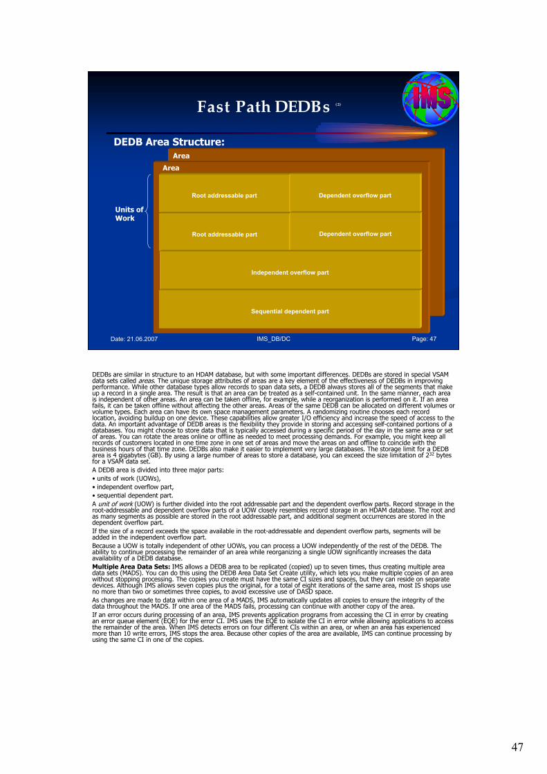
47
IMS_DB/DC Page: 47Date: 21.06.2007
Fast Path DEDBs (2)
DEDB Area Structure:
Root addressable part
Root addressable part
Dependent overflow part
Dependent overflow part
Independent overflow part
Sequential dependent part
Units of Work
Area
Area
DEDBs are similar in structure to an HDAM database, but with some important differences. DEDBs are stored in special VSAM data sets called areas. The unique storage attributes of areas are a key element of the effectiveness of DEDBs in improving performance. While other database types allow records to span data sets, a DEDB always stores all of the segments that make up a record in a single area. The result is that an area can be treated as a self-contained unit. In the same manner, each area is independent of other areas. An area can be taken offline, for example, while a reorganization is performed on it. If an area fails, it can be taken offline without affecting the other areas. Areas of the same DEDB can be allocated on different volumes or volume types. Each area can have its own space management parameters. A randomizing routine chooses each record location, avoiding buildup on one device. These capabilities allow greater I/O efficiency and increase the speed of access to the data. An important advantage of DEDB areas is the flexibility they provide in storing and accessing self-contained portions of a databases. You might choose to store data that is typically accessed during a specific period of the day in the same area or setof areas. You can rotate the areas online or offline as needed to meet processing demands. For example, you might keep all records of customers located in one time zone in one set of areas and move the areas on and offline to coincide with the business hours of that time zone. DEDBs also make it easier to implement very large databases. The storage limit for a DEDB area is 4 gigabytes (GB). By using a large number of areas to store a database, you can exceed the size limitation of 232 bytes for a VSAM data set.
A DEDB area is divided into three major parts:
• units of work (UOWs),
• independent overflow part,
• sequential dependent part.
A unit of work (UOW) is further divided into the root addressable part and the dependent overflow parts. Record storage in the root-addressable and dependent overflow parts of a UOW closely resembles record storage in an HDAM database. The root and as many segments as possible are stored in the root addressable part, and additional segment occurrences are stored in the dependent overflow part.
If the size of a record exceeds the space available in the root-addressable and dependent overflow parts, segments will be added in the independent overflow part.
Because a UOW is totally independent of other UOWs, you can process a UOW independently of the rest of the DEDB. The ability to continue processing the remainder of an area while reorganizing a single UOW significantly increases the data availability of a DEDB database.
Multiple Area Data Sets: IMS allows a DEDB area to be replicated (copied) up to seven times, thus creating multiple area data sets (MADS). You can do this using the DEDB Area Data Set Create utility, which lets you make multiple copies of an area without stopping processing. The copies you create must have the same CI sizes and spaces, but they can reside on separate devices. Although IMS allows seven copies plus the original, for a total of eight iterations of the same area, most IS shops useno more than two or sometimes three copies, to avoid excessive use of DASD space.
As changes are made to data within one area of a MADS, IMS automatically updates all copies to ensure the integrity of the data throughout the MADS. If one area of the MADS fails, processing can continue with another copy of the area.
If an error occurs during processing of an area, IMS prevents application programs from accessing the CI in error by creating an error queue element (EQE) for the error CI. IMS uses the EQE to isolate the CI in error while allowing applications to accessthe remainder of the area. When IMS detects errors on four different CIs within an area, or when an area has experienced more than 10 write errors, IMS stops the area. Because other copies of the area are available, IMS can continue processing by using the same CI in one of the copies.
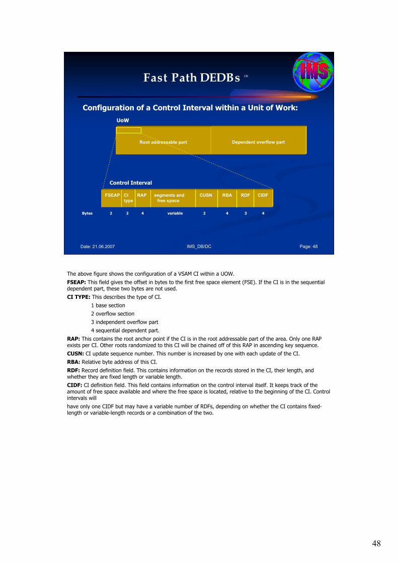
48
IMS_DB/DC Page: 48Date: 21.06.2007
Fast Path DEDBs (3)
Configuration of a Control Interval within a Unit of Work:
Root addressable part Dependent overflow part
UoW
Control Interval
FSEAP CI RAP segments and CUSN RBA RDF CIDF
type free space
Bytes 2 2 4 variable 2 4 3 4
The above figure shows the configuration of a VSAM CI within a UOW.
FSEAP: This field gives the offset in bytes to the first free space element (FSE). If the CI is in the sequential dependent part, these two bytes are not used.
CI TYPE: This describes the type of CI.
1 base section
2 overflow section
3 independent overflow part
4 sequential dependent part.
RAP: This contains the root anchor point if the CI is in the root addressable part of the area. Only one RAP exists per CI. Other roots randomized to this CI will be chained off of this RAP in ascending key sequence.
CUSN: CI update sequence number. This number is increased by one with each update of the CI.
RBA: Relative byte address of this CI.
RDF: Record definition field. This contains information on the records stored in the CI, their length, and whether they are fixed length or variable length.
CIDF: CI definition field. This field contains information on the control interval itself. It keeps track of the amount of free space available and where the free space is located, relative to the beginning of the CI. Control intervals will
have only one CIDF but may have a variable number of RDFs, depending on whether the CI contains fixed-length or variable-length records or a combination of the two.
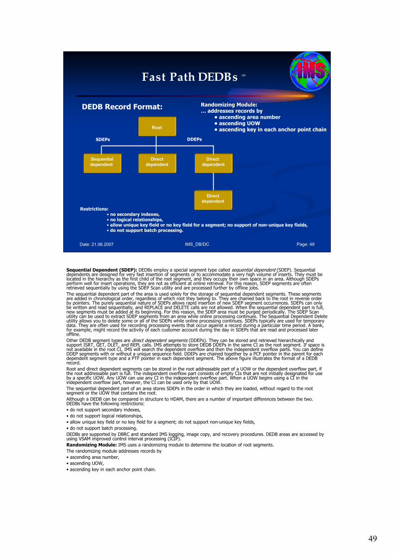
49
IMS_DB/DC Page: 49Date: 21.06.2007
Fast Path DEDBs (4)
DEDB Record Format:
Root
Direct
dependent
Sequential
dependent
Direct
dependent
Direct
dependent
DDEPsSDEPs
Restrictions:• no secondary indexes,• no logical relationships,• allow unique key field or no key field for a segment; no support of non-unique key fields,• do not support batch processing.
Randomizing Module: … addresses records by
• ascending area number• ascending UOW• ascending key in each anchor point chain
Sequential Dependent (SDEP): DEDBs employ a special segment type called sequential dependent (SDEP). Sequential dependents are designed for very fast insertion of segments or to accommodate a very high volume of inserts. They must be located in the hierarchy as the first child of the root segment, and they occupy their own space in an area. Although SDEPsperform well for insert operations, they are not as efficient at online retrieval. For this reason, SDEP segments are often retrieved sequentially by using the SDEP Scan utility and are processed further by offline jobs.
The sequential dependent part of the area is used solely for the storage of sequential dependent segments. These segments are added in chronological order, regardless of which root they belong to. They are chained back to the root in reverse order by pointers. The purely sequential nature of SDEPs allows rapid insertion of new SDEP segment occurrences. SDEPs can only be written and read sequentially, and REPLACE and DELETE calls are not allowed. When the sequential dependent part is full, new segments must be added at its beginning. For this reason, the SDEP area must be purged periodically. The SDEP Scan utility can be used to extract SDEP segments from an area while online processing continues. The Sequential Dependent Delete utility allows you to delete some or all of the SDEPs while online processing continues. SDEPs typically are used for temporary data. They are often used for recording processing events that occur against a record during a particular time period. A bank, for example, might record the activity of each customer account during the day in SDEPs that are read and processed later offline.
Other DEDB segment types are direct dependent segments (DDEPs). They can be stored and retrieved hierarchically and support ISRT, GET, DLET, and REPL calls. IMS attempts to store DEDB DDEPs in the same CI as the root segment. If space is not available in the root CI, IMS will search the dependent overflow and then the independent overflow parts. You can define DDEP segments with or without a unique sequence field. DDEPs are chained together by a PCF pointer in the parent for each dependent segment type and a PTF pointer in each dependent segment. The above figure illustrates the format of a DEDB record.
Root and direct dependent segments can be stored in the root addressable part of a UOW or the dependent overflow part, if the root addressable part is full. The independent overflow part consists of empty CIs that are not initially designated for use by a specific UOW. Any UOW can use any CI in the independent overflow part. When a UOW begins using a CI in the independent overflow part, however, the CI can be used only by that UOW.
The sequential dependent part of an area stores SDEPs in the order in which they are loaded, without regard to the root segment or the UOW that contains the root.
Although a DEDB can be compared in structure to HDAM, there are a number of important differences between the two. DEDBs have the following restrictions:
• do not support secondary indexes,
• do not support logical relationships,
• allow unique key field or no key field for a segment; do not support non-unique key fields,
• do not support batch processing.
DEDBs are supported by DBRC and standard IMS logging, image copy, and recovery procedures. DEDB areas are accessed by using VSAM improved control interval processing (ICIP).
Randomizing Module: IMS uses a randomizing module to determine the location of root segments.
The randomizing module addresses records by
• ascending area number,
• ascending UOW,
• ascending key in each anchor point chain.
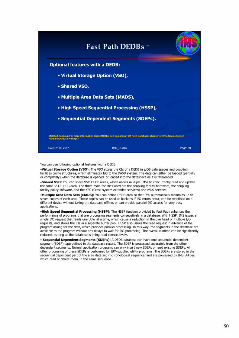
50
IMS_DB/DC Page: 50Date: 21.06.2007
Fast Path DEDBs (5)
Optional features with a DEDB:
• Virtual Storage Option (VSO),
• Shared VSO,
• Multiple Area Data Sets (MADS),
• High Speed Sequential Processing (HSSP),
• Sequential Dependent Segments (SDEPs).
Related Reading: For more information about DEDBs, see Designing Fast Path Databases chapter of IMS Administration Guide: Database Manager.
You can use following optional features with a DEDB:
•Virtual Storage Option (VSO): The VSO stores the CIs of a DEDB in z/OS data spaces and coupling facilities cache structures, which eliminates I/O to the DASD system. The data can either be loaded (partially or completely) when the database is opened, or loaded into the dataspace as it is referenced.
•Shared VSO: You can share VSO DEDB areas, which allows multiple IMSs to concurrently read and update the same VSO DEDB area. The three main facilities used are the coupling facility hardware, the coupling facility policy software, and the XES (Cross-system extended services) and z/OS services.
•Multiple Area Data Sets (MADS): You can define DEDB area so that IMS automatically maintains up to seven copies of each area. These copies can be used as backups if I/O errors occur, can be redefined on a different device without taking the database offline, or can provide parallel I/O access for very busy applications.
•High Speed Sequential Processing (HSSP): The HSSP function provided by Fast Path enhances the performance of programs that are processing segments consecutively in a database. With HSSP, IMS issues a single I/O request that reads one UoW at a time, which cause a reduction in the overhead of multiple I/O requests, and stores the CIs in a separate buffer pool. HSSP also issues the read request in advance of the program asking for the data, which provides parallel processing. In this way, the segments in the database are available to the program without any delays to wait for I/O processing. The overall runtime can be significantly reduced, as long as the database is being read consecutively.
• Sequential Dependent Segments (SDEPs): A DEDB database can have one sequential dependent segment (SDEP) type defined in the database record. The SDEP is processed separately from the other dependent segments. Normal application programs can only insert new SDEPs or read existing SDEPs. All other processing of these SDEPs is performed by IBM-supplied utility programs. The SDEPs are stored in the sequential dependent part of the area data set in chronological sequence, and are processed by IMS utilities, which read or delete them, in the same sequence.
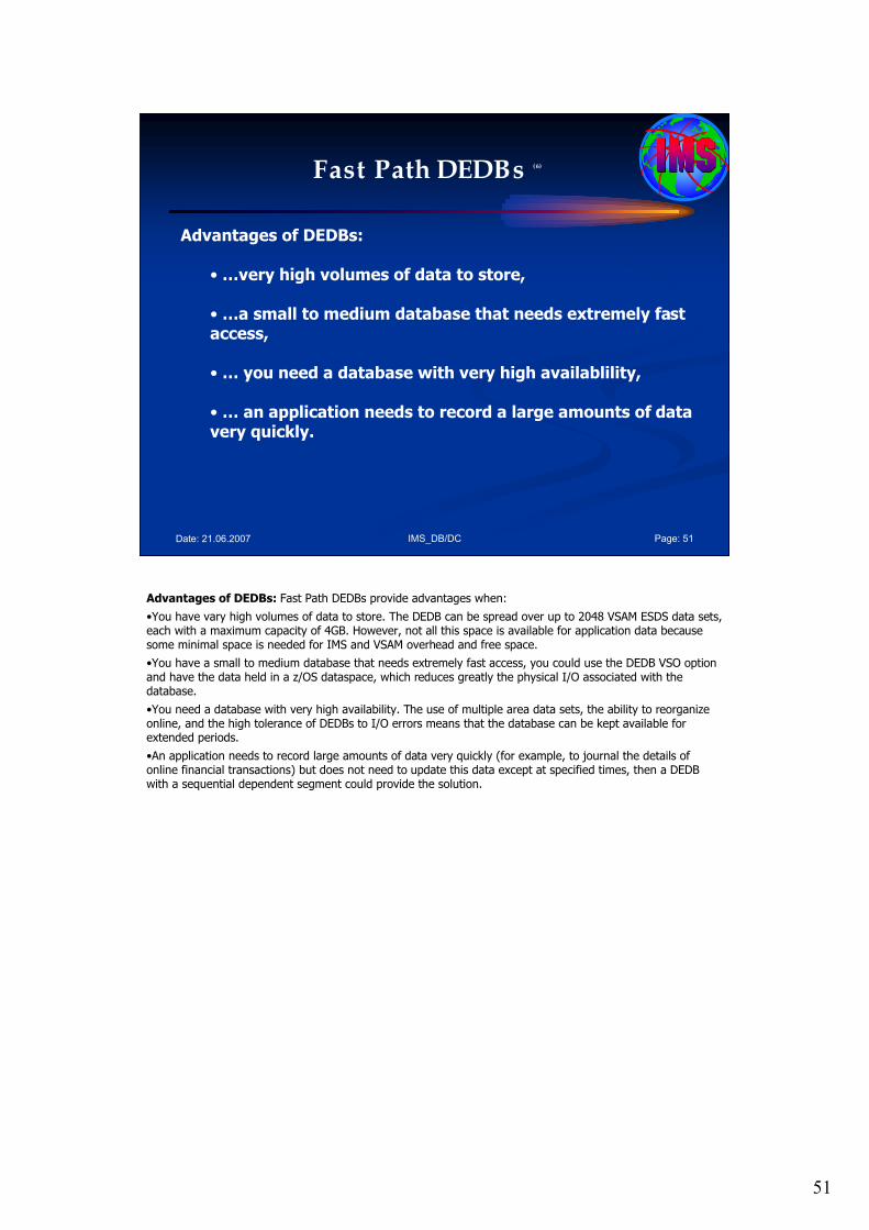
51
IMS_DB/DC Page: 51Date: 21.06.2007
Fast Path DEDBs (6)
Advantages of DEDBs:
•…very high volumes of data to store,
•…a small to medium database that needs extremely fast access,
•… you need a database with very high availablility,
•… an application needs to record a large amounts of data very quickly.
Advantages of DEDBs: Fast Path DEDBs provide advantages when:
•You have vary high volumes of data to store. The DEDB can be spread over up to 2048 VSAM ESDS data sets, each with a maximum capacity of 4GB. However, not all this space is available for application data because some minimal space is needed for IMS and VSAM overhead and free space.
•You have a small to medium database that needs extremely fast access, you could use the DEDB VSO option and have the data held in a z/OS dataspace, which reduces greatly the physical I/O associated with the database.
•You need a database with very high availability. The use of multiple area data sets, the ability to reorganize online, and the high tolerance of DEDBs to I/O errors means that the database can be kept available forextended periods.
•An application needs to record large amounts of data very quickly (for example, to journal the details of online financial transactions) but does not need to update this data except at specified times, then a DEDB with a sequential dependent segment could provide the solution.
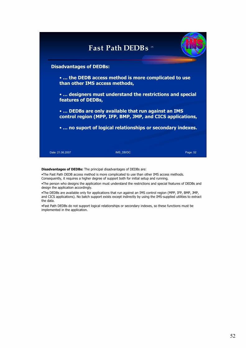
52
IMS_DB/DC Page: 52Date: 21.06.2007
Fast Path DEDBs (7)
Disadvantages of DEDBs:
•… the DEDB access method is more complicated to use than other IMS access methods,
•… designers must understand the restrictions and special features of DEDBs,
•… DEDBs are only available that run against an IMS control region (MPP, IFP, BMP, JMP, and CICS applications,
•… no suport of logical relationships or secondary indexes.
Disadvantages of DEDBs: The principal disadvantages of DEDBs are:
•The Fast Path DEDB access method is more complicated to use than other IMS access methods. Consequently, it requires a higher degree of support both for initial setup and running.
•The person who designs the application must understand the restrictions and special features of DEDBs and design the application accordingly.
•The DEDBs are available only for applications that run against an IMS control region (MPP, IFP, BMP, JMP, and CICS applications). No batch support exists except indirectly by using the IMS-supplied utilities to extract the data.
•Fast Path DEDBs do not support logical relationships or secondary indexes, so these functions must be implemented in the application.
53
IMS_DB/DC Page: 53Date: 21.06.2007
Fast Path DEDBs (8)
When to choose DEDBs:
• Advantages of areas,
• Understand when to use:
• VSO• MADS• HSSP• SDEPs
When to choose DEDBs: The art of knowing when to use a DEDB depends on understanding the differences between DEDBs and other database types. The following list describes some reasons and considerations for choosing DEDBS:
Advantages of areas: Most Fast Path commands and utilities operate on area level, so they do not affect the whole database at once (unlike full-function database). For example, you can recover one area of a DEDB while the rest of it is in use.
When to use - :
•VSO: Use VSO for your most frequently used databases, for those databases where fast access is crucial, and for data that is updated frequently, even if several applications want to update the same field at the same time. These considerations also apply to shared VSO.
•MADS: Use MADS to ensure that I/O errors do not affect a database. Normally two copies of each are is sufficient, but you can have up to seven copies if you need them. Using MADS is costly because you have several copies of the data. There is also a cost at execution time because IMS has to write several copies of the database updates. The transactions using the DEDB do not notice the extra I/O because the output threads handle the I/O operations asynchronously- Use MADS only when you can justify the extra DASD cost.
•HSSP: Use HSSP for only those programs that conform to its restrictions because you get better performance. Consider using the option to let HSSP take an image copy while it is running, which saves the time you would normally use to take an image copy after your program finishes.
•SDEPs: You would typically use SDEPs when you want to insert data quickly, but do not need to read it again until later. For example, you might want to use SDEPs to hold audit records describing sensitive actions the user takes. You would not use SDEPs to hold data for a long time.
54
IMS_DB/DC Page: 54Date: 21.06.2007
Agenda Session 3: Hierarchical Access Methods
1. HD Databases
• HDAM & HIDAM Access Method
• PHDAM & PHIDAM Access Methods
2. Index Databases
3. Fast Path DEDBs
4. GSAM Access Method
5. HS Databases
• HSAM & HISAM Access Method
6. Operating System Access Methods
7. Data Set Groups
8. Summary
4. GSAM Access Method.
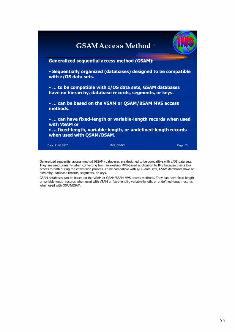
55
IMS_DB/DC Page: 55Date: 21.06.2007
GSAM Access Method (1)
Generalized sequential access method (GSAM):
• Sequentially organized (databases) designed to be compatible with z/OS data sets.
•… to be compatible with z/OS data sets, GSAM databases have no hierarchy, database records, segments, or keys.
•… can be based on the VSAM or QSAM/BSAM MVS access methods.
•… can have fixed-length or variable-length records when used with VSAM or •… fixed-length, variable-length, or undefined-length records when used with QSAM/BSAM.
Generalized sequential access method (GSAM) databases are designed to be compatible with z/OS data sets. They are used primarily when converting from an existing MVS-based application to IMS because they allow access to both during the conversion process. To be compatible with z/OS data sets, GSAM databases have no hierarchy, database records, segments, or keys.
GSAM databases can be based on the VSAM or QSAM/BSAM MVS access methods. They can have fixed-length or variable-length records when used with VSAM or fixed-length, variable-length, or undefined-length records when used with QSAM/BSAM.
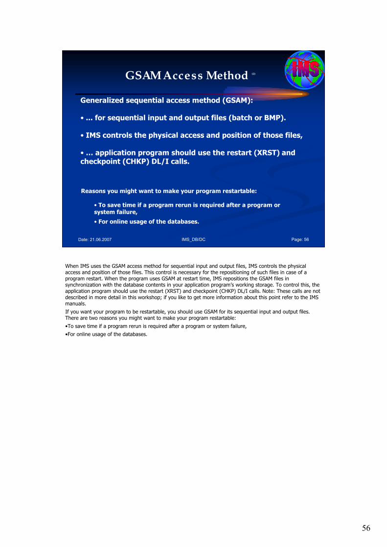
56
IMS_DB/DC Page: 56Date: 21.06.2007
GSAM Access Method (2)
Generalized sequential access method (GSAM):
• ... for sequential input and output files (batch or BMP).
• IMS controls the physical access and position of those files,
•… application program should use the restart (XRST) and checkpoint (CHKP) DL/I calls.
Reasons you might want to make your program restartable:
• To save time if a program rerun is required after a program or system failure,
• For online usage of the databases.
When IMS uses the GSAM access method for sequential input and output files, IMS controls the physical access and position of those files. This control is necessary for the repositioning of such files in case of a program restart. When the program uses GSAM at restart time, IMS repositions the GSAM files in synchronization with the database contents in your application program’s working storage. To control this, the application program should use the restart (XRST) and checkpoint (CHKP) DL/I calls. Note: These calls are not described in more detail in this workshop; if you like to get more information about this point refer to the IMS manuals.
If you want your program to be restartable, you should use GSAM for its sequential input and output files.There are two reasons you might want to make your program restartable:
•To save time if a program rerun is required after a program or system failure,
•For online usage of the databases.
57
IMS_DB/DC Page: 57Date: 21.06.2007
Agenda Session 3: Hierarchical Access Methods
1. HD Databases
• HDAM & HIDAM Access Method
• PHDAM & PHIDAM Access Methods
2. Index Databases
3. Fast Path DEDBs
4. GSAM Access Method
5. HS Databases• HSAM & HISAM Access Method
6. Operating System Access Methods
7. Data Set Groups
8. Summary
5.HS Databases.
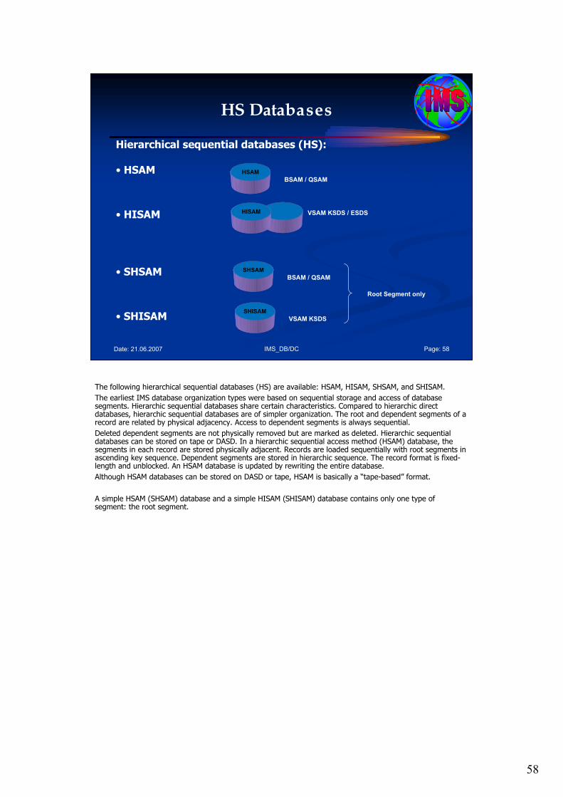
58
IMS_DB/DC Page: 58Date: 21.06.2007
HS Databases
Hierarchical sequential databases (HS):
• HSAM
• HISAM
• SHSAM
• SHISAM
HSAM
BSAM / QSAM
HISAM VSAM KSDS / ESDS
SHSAM
BSAM / QSAM
SHISAM
VSAM KSDS
Root Segment only
The following hierarchical sequential databases (HS) are available: HSAM, HISAM, SHSAM, and SHISAM.
The earliest IMS database organization types were based on sequential storage and access of database segments. Hierarchic sequential databases share certain characteristics. Compared to hierarchic direct databases, hierarchic sequential databases are of simpler organization. The root and dependent segments of a record are related by physical adjacency. Access to dependent segments is always sequential.
Deleted dependent segments are not physically removed but are marked as deleted. Hierarchic sequential databases can be stored on tape or DASD. In a hierarchic sequential access method (HSAM) database, the segments in each record are stored physically adjacent. Records are loaded sequentially with root segments in ascending key sequence. Dependent segments are stored in hierarchic sequence. The record format is fixed-length and unblocked. An HSAM database is updated by rewriting the entire database.
Although HSAM databases can be stored on DASD or tape, HSAM is basically a “tape-based” format.
A simple HSAM (SHSAM) database and a simple HISAM (SHISAM) database contains only one type of segment: the root segment.

59
IMS_DB/DC Page: 59Date: 21.06.2007
Agenda Session 3: Hierarchical Access Methods
1. HD Databases
• HDAM & HIDAM Access Method
• PHDAM & PHIDAM Access Methods
2. Index Databases
3. Fast Path DEDBs
4. GSAM Access Method
5. HS Databases• HSAM & HISAM Access Method
6. Operating System Access Methods
7. Data Set Groups
8. Summary
HS Databases: HSAM & HISAM Access Method
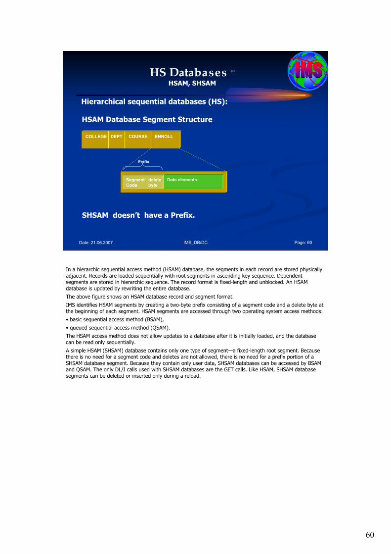
60
IMS_DB/DC Page: 60Date: 21.06.2007
HS Databases (1)
HSAM, SHSAM
Hierarchical sequential databases (HS):
COLLEGE DEPT COURSE ENROLL
HSAM Database Segment Structure
Segment delete
Code byte
Data elements
Prefix
SHSAM doesn’t have a Prefix.
In a hierarchic sequential access method (HSAM) database, the segments in each record are stored physically adjacent. Records are loaded sequentially with root segments in ascending key sequence. Dependent segments are stored in hierarchic sequence. The record format is fixed-length and unblocked. An HSAM database is updated by rewriting the entire database.
The above figure shows an HSAM database record and segment format.
IMS identifies HSAM segments by creating a two-byte prefix consisting of a segment code and a delete byte at the beginning of each segment. HSAM segments are accessed through two operating system access methods:
• basic sequential access method (BSAM),
• queued sequential access method (QSAM).
The HSAM access method does not allow updates to a database after it is initially loaded, and the database can be read only sequentially.
A simple HSAM (SHSAM) database contains only one type of segment—a fixed-length root segment. Because there is no need for a segment code and deletes are not allowed, there is no need for a prefix portion of a SHSAM database segment. Because they contain only user data, SHSAM databases can be accessed by BSAM and QSAM. The only DL/I calls used with SHSAM databases are the GET calls. Like HSAM, SHSAM database segments can be deleted or inserted only during a reload.
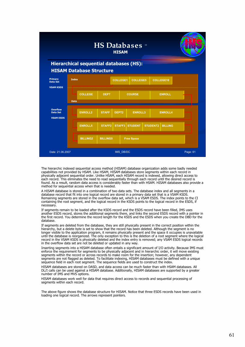
61
IMS_DB/DC Page: 61Date: 21.06.2007
HS Databases (2)
HISAM
Hierarchical sequential databases (HS):
HISAM Database Structure
COLLEGE1 COLLEGE5 COLLEGE10
COLLEGE DEPT COURSE ENROLL
ENROLL2 STAFF DEPT2 ENROLL3 ENROLL4
ENROLL5 STAFF2 STAFF3 STUDENT STUDENT2 BILLING
BILLING2 BILLING5 Free Space
Index
Data
PrimaryData Set
VSAM KSDS
OverflowData Set
VSAM ESDS
The hierarchic indexed sequential access method (HISAM) database organization adds some badly needed capabilities not provided by HSAM. Like HSAM, HISAM databases store segments within each record in physically adjacent sequential order. Unlike HSAM, each HISAM record is indexed, allowing direct access to each record. This eliminates the need to read sequentially through each record until the desired record is found. As a result, random data access is considerably faster than with HSAM. HISAM databases also provide a method for sequential access when that is needed.
A HISAM database is stored in a combination of two data sets. The database index and all segments in a database record that fit into one logical record are stored in a primary data set that is a VSAM KSDS. Remaining segments are stored in the overflow data set, which is a VSAM ESDS. The index points to the CI containing the root segment, and the logical record in the KSDS points to the logical record in the ESDS, if necessary.
If segments remain to be loaded after the KSDS record and the ESDS record have been filled, IMS uses another ESDS record, stores the additional segments there, and links the second ESDS record with a pointer in the first record. You determine the record length for the KSDS and the ESDS when you create the DBD for the database.
If segments are deleted from the database, they are still physically present in the correct position within the hierarchy, but a delete byte is set to show that the record has been deleted. Although the segment is no longer visible to the application program, it remains physically present and the space it occupies is unavailable until the database is reorganized. The only exception to this is the deletion of a root segment where the logical record in the VSAM KSDS is physically deleted and the index entry is removed; any VSAM ESDS logical records in the overflow data set are not be deleted or updated in any way.
Inserting segments into a HISAM database often entails a significant amount of I/O activity. Because IMS must enforce the requirement for segments to be physically adjacent and in hierarchic order, it will move existing segments within the record or across records to make room for the insertion; however, any dependent segments are not flagged as deleted. To facilitate indexing, HISAM databases must be defined with a unique sequence field in each root segment. The sequence fields are used to construct the index.
HISAM databases are stored on DASD, and data access can be much faster than with HSAM databases. All DL/I calls can be used against a HISAM database. Additionally, HISAM databases are supported by a greater number of IMS and MVS options.
HISAM databases work well for data that requires direct access to records and sequential processing of segments within each record.
The above figure shows the database structure for HISAM. Notice that three ESDS records have been used in loading one logical record. The arrows represent pointers.
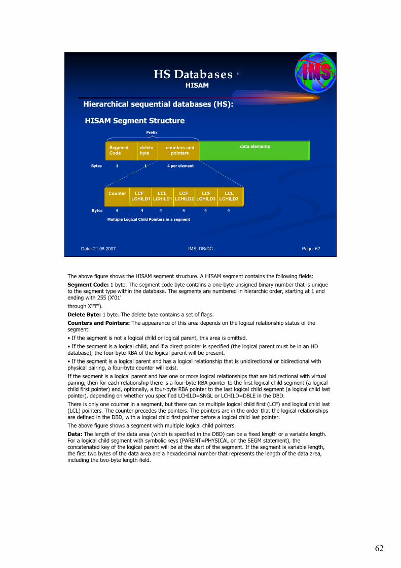
62
IMS_DB/DC Page: 62Date: 21.06.2007
HS Databases (3)
HISAM
Hierarchical sequential databases (HS):
HISAM Segment Structure
Segment delete counters and
Code byte pointers
Prefix
Bytes 1 1 4 per element
data elements
Counter LCF LCL LCF LCF LCL
LCHILD1 LCHILD1 LCHILD2 LCHILD3 LCHILD3
Multiple Logical Child Pointers in a segment
Bytes 4 4 4 4 4 4
The above figure shows the HISAM segment structure. A HISAM segment contains the following fields:
Segment Code: 1 byte. The segment code byte contains a one-byte unsigned binary number that is unique to the segment type within the database. The segments are numbered in hierarchic order, starting at 1 and ending with 255 (X'01'
through X'FF').
Delete Byte: 1 byte. The delete byte contains a set of flags.
Counters and Pointers: The appearance of this area depends on the logical relationship status of the segment:
• If the segment is not a logical child or logical parent, this area is omitted.
• If the segment is a logical child, and if a direct pointer is specified (the logical parent must be in an HD database), the four-byte RBA of the logical parent will be present.
• If the segment is a logical parent and has a logical relationship that is unidirectional or bidirectional with physical pairing, a four-byte counter will exist.
If the segment is a logical parent and has one or more logical relationships that are bidirectional with virtual pairing, then for each relationship there is a four-byte RBA pointer to the first logical child segment (a logical child first pointer) and, optionally, a four-byte RBA pointer to the last logical child segment (a logical child last pointer), depending on whether you specified LCHILD=SNGL or LCHILD=DBLE in the DBD.
There is only one counter in a segment, but there can be multiple logical child first (LCF) and logical child last (LCL) pointers. The counter precedes the pointers. The pointers are in the order that the logical relationships are defined in the DBD, with a logical child first pointer before a logical child last pointer.
The above figure shows a segment with multiple logical child pointers.
Data: The length of the data area (which is specified in the DBD) can be a fixed length or a variable length. For a logical child segment with symbolic keys (PARENT=PHYSICAL on the SEGM statement), the concatenated key of the logical parent will be at the start of the segment. If the segment is variable length, the first two bytes of the data area are a hexadecimal number that represents the length of the data area, including the two-byte length field.
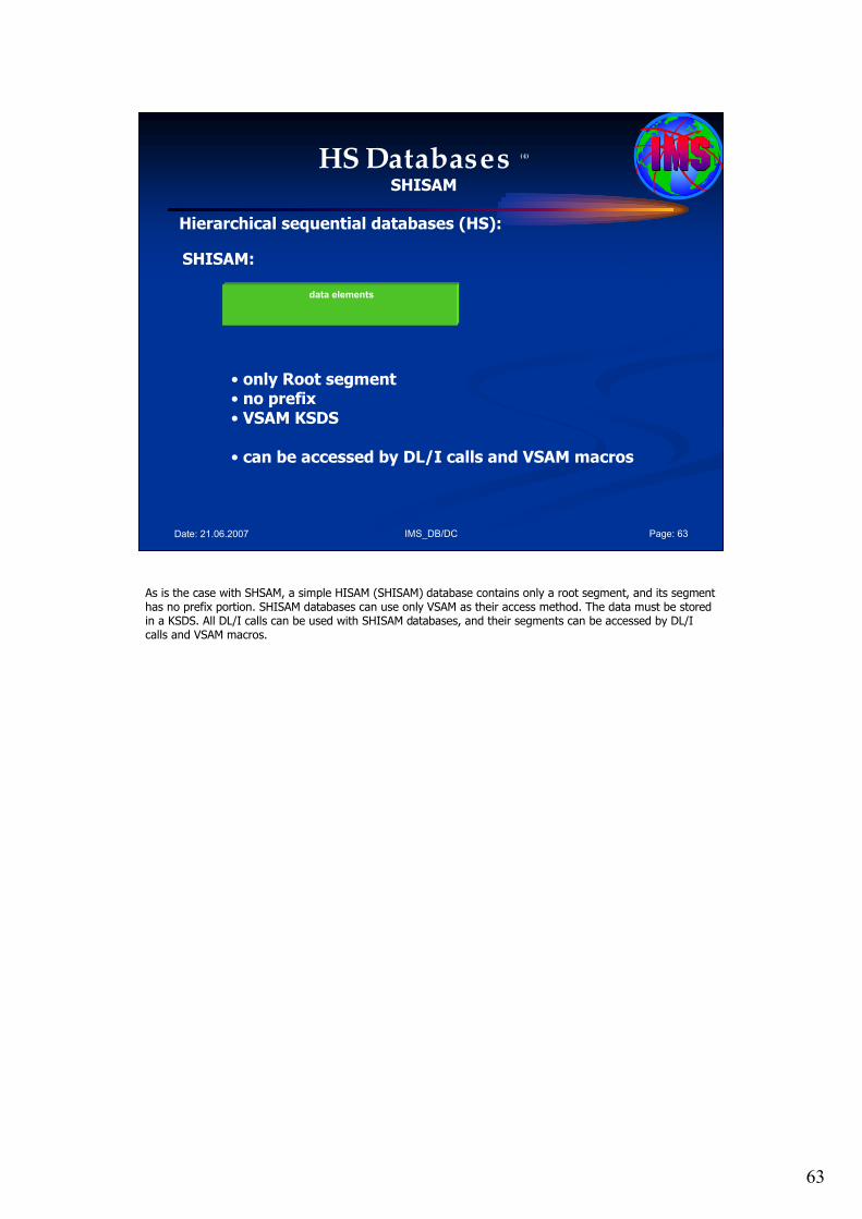
63
IMS_DB/DC Page: 63Date: 21.06.2007
HS Databases (4)
SHISAM
Hierarchical sequential databases (HS):
SHISAM:
data elements
• only Root segment• no prefix• VSAM KSDS
• can be accessed by DL/I calls and VSAM macros
As is the case with SHSAM, a simple HISAM (SHISAM) database contains only a root segment, and its segment has no prefix portion. SHISAM databases can use only VSAM as their access method. The data must be stored in a KSDS. All DL/I calls can be used with SHISAM databases, and their segments can be accessed by DL/I calls and VSAM macros.
64
IMS_DB/DC Page: 64Date: 21.06.2007
HS Databases (5)
HSAM, SHSAM, HISAM, SHISAM
Hierarchical sequential databases (HS):
Recommendations using HISAM:
1. Database records are relatively small,2. Database records are relatively uniform in size,3. The database is stable,4. … will not grow past 4GB.
Recommendations using SHISAM:
1. …meets the SHISAM restrictions,2. … process a KSDS with fixed length records as an IMS
database.
Recommendations for using HISAM:
1. Database records are relatively small. They typically require only one logical record in the primary data set (KSDS). Occasionally, they might require one logical record in the overflow area (ESDS).
2. Database records are relatively uniform in site. There is not a large range in size for most database records.
3. The database is stable. There are not high volumes of deletes and inserts in the database.
4. The database will not grow past the data set size limitations of 4GB per dataset.
Recommendations using SHISAM:
1. If you have a database which meets the SHISAM restrictions, you should consider using SHISAM for it.
2. Additionally, if you need to process a KSDS with fixed length records as an IMS database, you may define it as SHISAM.
65
IMS_DB/DC Page: 65Date: 21.06.2007
HS Databases (6)
HSAM, SHSAM, HISAM, SHISAM
Hierarchical sequential databases (HS):
Applications that are suitable for HSAM and HISAM:
• HSAM - … has been superseded (replaced by GSAM) ,• no update, read only sequentially
• HISAM - … is not an effective database organization type,• may be reorganized much more frequently
• SHSAM and SHISAM - … has only root segments.
HSAM is one of the original database access methods and has been superseded. It is rarely used today.
HISAM is not an effective database organization type. You can easily convert HISAM databases to HIDAM. Applications should receive significant performance improvements as a result. The only situation where HISAM might be preferable to HIDAM is when the database is a root-segment-only database or where there is only very poor insert or delete activity (for example in archive DBs).
An example of the inefficiency of HISAM is that segments are not completely deleted and free space is not reclaimed after a segment is deleted until the next database reorganization.
66
IMS_DB/DC Page: 66Date: 21.06.2007
Agenda Session 3: Hierarchical Access Methods
1. HD Databases
• HDAM & HIDAM Access Method
• PHDAM & PHIDAM Access Methods
2. Index Databases
3. Fast Path DEDBs
4. GSAM Access Method
5. HS Databases
• HSAM & HISAM Access Method
6. Operating System Access Methods
7. Data Set Groups
8. Summary
6. Operating System Access Methods.

67
IMS_DB/DC Page: 67Date: 21.06.2007
Operating System Access Methods
Operating System Access Methods:
• Virtual Storage Access Method (VSAM)• KSDS, ESDS,
• Overflow Sequential Access Method (OSAM)• DSORG=PS ,
• the VSAM and OSAM access methods define two types of datasets:
• Indexed sequential data sets• VSAM KSDS
• Sequential data sets• VSAM ESDS or OSAM
IMS uses two operating system methods to physically store the data on disk storage and move the data between the disk storage and the buffers in the IMS address space:
•Virtual Storage Access Method (VSAM): IMS uses two of the available VSAM access methods:
•Key-sequenced data sets (KSDSs) are used for index and HISAM databases,
•Entry-sequenced data sets (ESDSs) are used for the primary data sets for HDAM, HIDAM, PHDAM, and PHIDAM databases. The data sets are defined using VSAM Access Method Services (AMS) utility program.
•Overflow Sequential Access Method (OSAM): The OSAM access method is unique to IMS, is delivered as part of the IMS product, and consists of a series of channel programs that IMS executes to use the standard operating system channel I/O interface. The OSAM data sets are defined using JCL statements, To the operating system, an OSAM data set is described as a physical sequential data set /DSORG=PS).
The VSAM and OSAM access methods define two types of data sets:
•Indexed sequential data sets: Defined and accessed as VSAM KSDSs, are used to implement primary and secondary index databases. The index databases are processed using the standard record level instructions of VSAM. A catalog listing (VSAM LISTCAT) shows all current details of the files. VSAM KSDSs are susceptible to the normal performance degradation from CI or CA splits caused by insert and delete activity. VSAM KSDSscan, if necessary, be processed using AMS utilties such as REPRO.
•Sequential data sets: Defined and accessed either as VSAM ESDSs or using OSAM. While these data sets appear as sequential data sets to the operating system, IMS accesses them randomly, therefore the data sets do not contain records. IMS always processes them at the CI (VSAM) or block (OSAM) level. The internal structure within each CI or block is arranged as described earlier in “IMS Hierarchical Access Methods”. Interpreting catalog listings of these files as if they were sequential files can, therefore, be misleading.
In addition to using VSAM or OSAM, most IMS data sets can be managed by Data Facility Storage Management Subsystem (DFSMS).
The exception is the datasets that IMS uses for logging (This is not a part of this workshop!).
68
IMS_DB/DC Page: 68Date: 21.06.2007
Agenda Session 3: Hierarchical Access Methods
1. HD Databases
• HDAM & HIDAM Access Method
• PHDAM & PHIDAM Access Methods
2. Index Databases
3. Fast Path DEDBs
4. GSAM Access Method
5. HS Databases
• HSAM & HISAM Access Method
6. Operating System Access Methods
7. Data Set Groups
8. Summary
7. Data Set Groups.
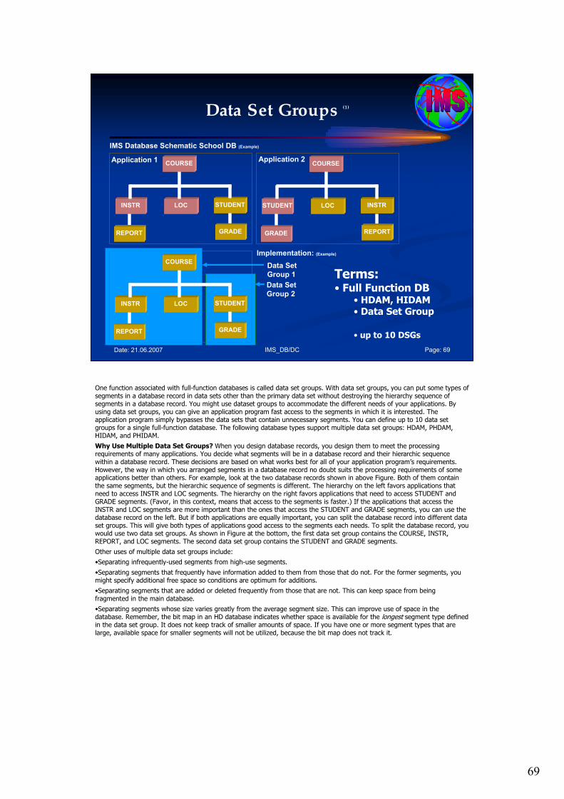
69
IMS_DB/DC Page: 69Date: 21.06.2007
Data Set Groups (1)
Terms:• Full Function DB
• HDAM, HIDAM• Data Set Group
• up to 10 DSGs
IMS Database Schematic School DB (Example)
COURSE
INSTR LOC STUDENT
REPORT GRADE
Application 1COURSE
STUDENT LOC INSTR
GRADE REPORT
Application 2
COURSE
INSTR LOC STUDENT
REPORT GRADE
Data Set
Group 1
Data Set
Group 2
Implementation: (Example)
One function associated with full-function databases is called data set groups. With data set groups, you can put some types of segments in a database record in data sets other than the primary data set without destroying the hierarchy sequence of segments in a database record. You might use dataset groups to accommodate the different needs of your applications. By using data set groups, you can give an application program fast access to the segments in which it is interested. The application program simply bypasses the data sets that contain unnecessary segments. You can define up to 10 data set groups for a single full-function database. The following database types support multiple data set groups: HDAM, PHDAM, HIDAM, and PHIDAM.
Why Use Multiple Data Set Groups? When you design database records, you design them to meet the processing requirements of many applications. You decide what segments will be in a database record and their hierarchic sequence within a database record. These decisions are based on what works best for all of your application program’s requirements. However, the way in which you arranged segments in a database record no doubt suits the processing requirements of some applications better than others. For example, look at the two database records shown in above Figure. Both of them contain the same segments, but the hierarchic sequence of segments is different. The hierarchy on the left favors applications that need to access INSTR and LOC segments. The hierarchy on the right favors applications that need to access STUDENT and GRADE segments. (Favor, in this context, means that access to the segments is faster.) If the applications that access the INSTR and LOC segments are more important than the ones that access the STUDENT and GRADE segments, you can use the database record on the left. But if both applications are equally important, you can split the database record into different data set groups. This will give both types of applications good access to the segments each needs. To split the database record, you would use two data set groups. As shown in Figure at the bottom, the first data set group contains the COURSE, INSTR, REPORT, and LOC segments. The second data set group contains the STUDENT and GRADE segments.
Other uses of multiple data set groups include:
•Separating infrequently-used segments from high-use segments.
•Separating segments that frequently have information added to them from those that do not. For the former segments, you might specify additional free space so conditions are optimum for additions.
•Separating segments that are added or deleted frequently from those that are not. This can keep space from being fragmented in the main database.
•Separating segments whose size varies greatly from the average segment size. This can improve use of space in the database. Remember, the bit map in an HD database indicates whether space is available for the longest segment type defined in the data set group. It does not keep track of smaller amounts of space. If you have one or more segment types that are large, available space for smaller segments will not be utilized, because the bit map does not track it.
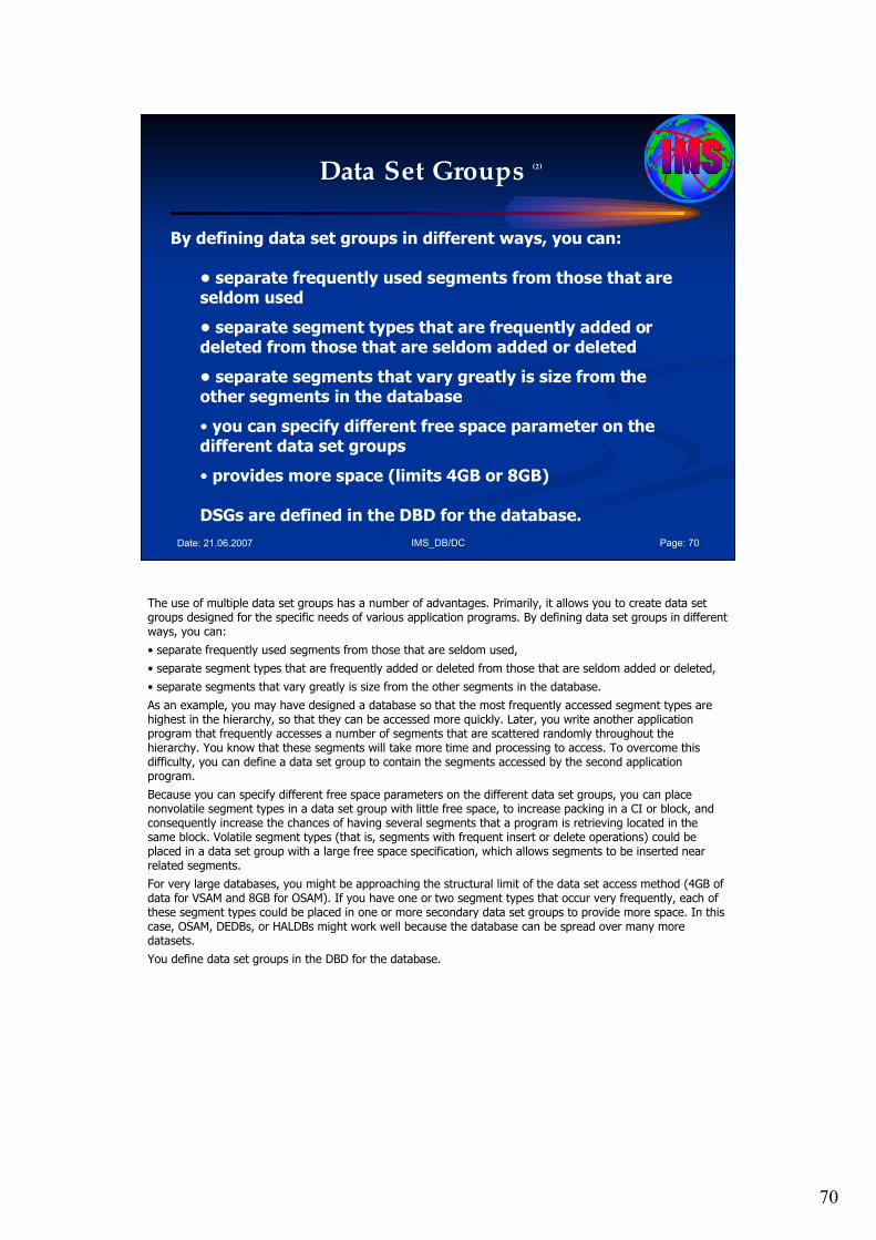
70
IMS_DB/DC Page: 70Date: 21.06.2007
Data Set Groups (2)
By defining data set groups in different ways, you can:
• separate frequently used segments from those that are seldom used
• separate segment types that are frequently added or deleted from those that are seldom added or deleted
• separate segments that vary greatly is size from the other segments in the database
• you can specify different free space parameter on the different data set groups
• provides more space (limits 4GB or 8GB)
DSGs are defined in the DBD for the database.
The use of multiple data set groups has a number of advantages. Primarily, it allows you to create data set groups designed for the specific needs of various application programs. By defining data set groups in different ways, you can:
• separate frequently used segments from those that are seldom used,
• separate segment types that are frequently added or deleted from those that are seldom added or deleted,
• separate segments that vary greatly is size from the other segments in the database.
As an example, you may have designed a database so that the most frequently accessed segment types are highest in the hierarchy, so that they can be accessed more quickly. Later, you write another application program that frequently accesses a number of segments that are scattered randomly throughout the hierarchy. You know that these segments will take more time and processing to access. To overcome this difficulty, you can define a data set group to contain the segments accessed by the second application program.
Because you can specify different free space parameters on the different data set groups, you can place nonvolatile segment types in a data set group with little free space, to increase packing in a CI or block, and consequently increase the chances of having several segments that a program is retrieving located in the same block. Volatile segment types (that is, segments with frequent insert or delete operations) could be placed in a data set group with a large free space specification, which allows segments to be inserted near related segments.
For very large databases, you might be approaching the structural limit of the data set access method (4GB of data for VSAM and 8GB for OSAM). If you have one or two segment types that occur very frequently, each of these segment types could be placed in one or more secondary data set groups to provide more space. In this case, OSAM, DEDBs, or HALDBs might work well because the database can be spread over many more datasets.
You define data set groups in the DBD for the database.
71
IMS_DB/DC Page: 71Date: 21.06.2007
Data Set Groups (3)
Restrictions / Considerations:
• … the first (primary) data set group must contain the root segments, and can optionally contain any dependent segment type.
•… each dependent segment type can be defined only in one data set group.
•… DSGs are not transparent to application programs.
•… Reorganization is done for the complete DB.
Following restrictions and/or considerations apply to DSGs:
One of the restrictions associated with data set groups is that the first (primary) data set group that is defined must contain the root segments, and can optionally contain any dependent segment type. The other (or secondary) data set groups can each contain any dependent segment type. However, each dependent segment type can be defined in only one data set group. These restrictions, aside from performance implications, are not transparent to applications. If the database must be reorganized, then all datasets that make up the physical database must be reorganized at the same time.
72
IMS_DB/DC Page: 72Date: 21.06.2007
Data Set Groups (4)
VSAM versus OSAM for Data Set Groups:
•… it depends,
•… change is possible through Unloading the database, changing and regenerating the DBD, then reloading the database,
•… OSAM may have some advantages•… sequential buffering (SB),•… space limit (8GB),•… more efficient than VSAM ESDSs -> shorter instruction path
The choice between OSAM and VSAM ESDSs for the primary database data sets depends, to some extent, on whether your site already uses VSAM and whether you need to make use of the additional features of OSAM. The choice between VSAM ESDSs and OSAM is not final because you can change a database from on access method to the other by unloading the database, changing and regenerating the DBD, then reloading the database.
Because the OSAM access method is specified to IMS, it is optimized for use by IMS. The reasons you might want to use OSAM include:
•The availability of sequential buffering (SB). With sequential buffering, IMS detects when an application is physically processing data sequentially or consecutively and fetches in advance any blocks it expects the application to request from DASD, so that the blocks are already in the buffers in the IMS address space when the application requests segments in the blocks. Sequential buffering is manually activated for specific IMS databases and programs and can appreciably increase performance for applications that physically process databases sequentially or consecutively. Sequential buffering is similar to the sequential prefetch that is available with some DASD controllers, but has the advantage that the data is fetched into the address space buffers in main memory rather than the DASD controller cache at the other end of the channel.
•The structural limit on the amount of data that IMS can store in a VSAM ESDS is 4GB of data. OSAM can process a data set up to 8 GB in size.
•Overall, OSAM is regarded as more efficient than VSAM ESDSs because OSAM has a shorter instruction path.
73
IMS_DB/DC Page: 73Date: 21.06.2007
Data Set Groups (5)
Recommendations Summary for Multiple Data Set Groups:
1. Define multiple data set groups only when you have a reason to do so.
2. You may use multiple data set groups to provide additional capacity for HDAM and HIDAM databases.
3. Do not use multiple data set groups with PHDAM and PHIDAM to provide capacity; instead, create more partitions.
The recommendations for the use of multiple data set groups are:
1. Define multiple data set groups only when you have a reason to do so. You should use them primarily to reduce I/Os for database with certain characteristics.
2. You may use multiple data set groups to provide additional capacity for HDAM and HIDAM databases, but conversion to PHDAM and PHIDAM is preferable.
3. Do not use multiple data set groups with PHDAM and PHIDAM databases to provide capacity. Instead, create more partitions for these databases. Multiple data set groups may be appropriate for PHDAM or PHIDAM databases to reduce I/Os.
74
IMS_DB/DC Page: 74Date: 21.06.2007
Agenda Session 3: Hierarchical Access Methods
1. HD Databases
• HDAM & HIDAM Access Method
• PHDAM & PHIDAM Access Methods
2. Index Databases
3. Fast Path DEDBs
4. GSAM Access Method
5. HS Databases
• HSAM & HISAM Access Method
6. Operating System Access Methods
7. Data Set Groups
8. Summary
8. Summary.
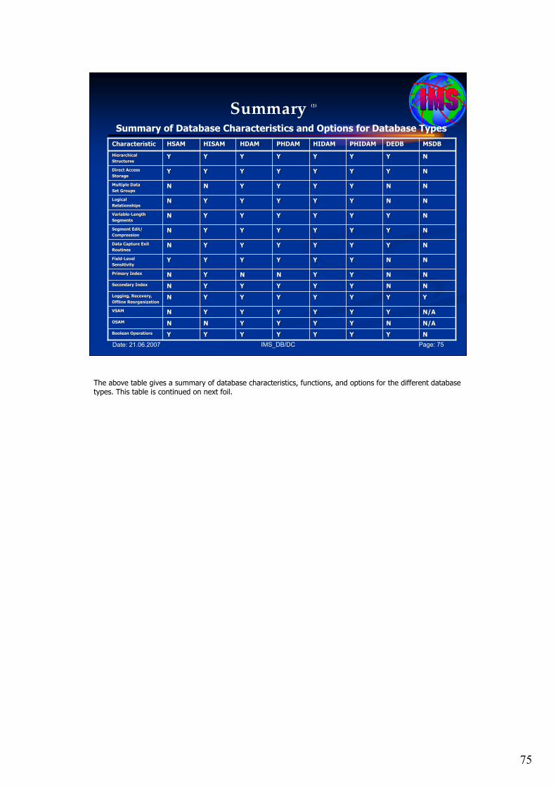
75
IMS_DB/DC Page: 75Date: 21.06.2007
Summary (1)
Summary of Database Characteristics and Options for Database Types
NNYYYYYYYYYYYYYYBoolean Boolean OperatiorsOperatiors
N/AN/ANNYYYYYYYYNNNNOSAMOSAM
N/AN/AYYYYYYYYYYYYNNVSAMVSAM
YYYYYYYYYYYYYYNNLogging, Recovery,Logging, Recovery,
Offline ReorganizationOffline Reorganization
NNNNYYYYYYYYYYNNSecondary IndexSecondary Index
NNNNYYYYNNNNYYNNPrimary IndexPrimary Index
NNNNYYYYYYYYYYYYFieldField--LevelLevel
SensitivitySensitivity
NNYYYYYYYYYYYYNNData Capture ExitData Capture Exit
RoutinesRoutines
NNYYYYYYYYYYYYNNSegment Edit/Segment Edit/
CompressionCompression
NNYYYYYYYYYYYYNNVariableVariable--LengthLength
SegmentsSegments
NNNNYYYYYYYYYYNNLogical Logical
RelationshipsRelationships
NNNNYYYYYYYYNNNNMultiple DataMultiple Data
Set GroupsSet Groups
NNYYYYYYYYYYYYYYDirect AccessDirect Access
StorageStorage
NNYYYYYYYYYYYYYYHierarchicalHierarchical
StructuresStructures
MSDBMSDBDEDBDEDBPHIDAMPHIDAMHIDAMHIDAMPHDAMPHDAMHDAMHDAMHISAMHISAMHSAMHSAMCharacteristicCharacteristic
The above table gives a summary of database characteristics, functions, and options for the different database types. This table is continued on next foil.
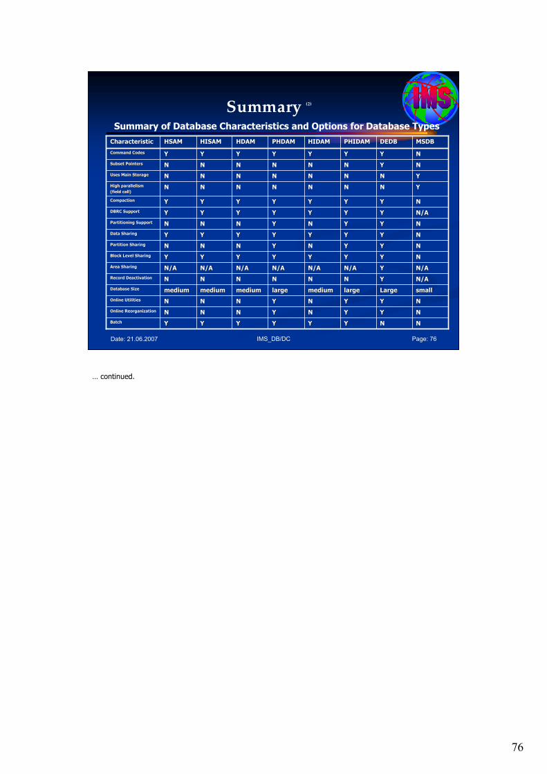
76
IMS_DB/DC Page: 76Date: 21.06.2007
Summary (2)
Summary of Database Characteristics and Options for Database Types
NNNNYYYYYYYYYYYYBatchBatch
NNYYYYNNYYNNNNNNOnline ReorganizationOnline Reorganization
NNYYYYNNYYNNNNNNOnline UtilitiesOnline Utilities
smallsmallLargeLargelargelargemediummediumlargelargemediummediummediummediummediummediumDatabase SizeDatabase Size
N/AN/AYYNNNNNNNNNNNNRecord DeactivationRecord Deactivation
N/AN/AYYN/AN/AN/AN/AN/AN/AN/AN/AN/AN/AN/AN/AArea SharingArea Sharing
NNYYYYYYYYYYYYYYBlock Level SharingBlock Level Sharing
NNYYYYNNYYNNNNNNPartition SharingPartition Sharing
NNYYYYYYYYYYYYYYData SharingData Sharing
NNYYYYNNYYNNNNNNPartitioning SupportPartitioning Support
N/AN/AYYYYYYYYYYYYYYDBRC SupportDBRC Support
NNYYYYYYYYYYYYYYCompactionCompaction
YYNNNNNNNNNNNNNNHigh parallelismHigh parallelism
(field call)(field call)
YYNNNNNNNNNNNNNNUses Main StorageUses Main Storage
NNYYNNNNNNNNNNNNSubset PointersSubset Pointers
NNYYYYYYYYYYYYYYCommand CodesCommand Codes
MSDBMSDBDEDBDEDBPHIDAMPHIDAMHIDAMHIDAMPHDAMPHDAMHDAMHDAMHISAMHISAMHSAMHSAMCharacteristicCharacteristic
… continued.
77
IMS_DB/DC Page: 77Date: 21.06.2007
Source
See: • IBM Web page
http://www-306.ibm.com/software/data/ims/
IMS Administration Guide: Database Manager
and the IBM Redbook: The Complete IMS HALDB Guide All You Need to
Know to Manage HALDBs.
For more information about DEDBs, see Designing Fast Path Databases chapter
of IMS Administration Guide: Database Manager.
• BookAn Introduction to IMS, IBM Press
In all sessions I like to motivate you to study additional books and publications about IMS DB/DC.

78
Date: 21.06.2007 IMS_03_3.ppt Page: 78
Questions / CommentsQuestions / Comments……
? ? ?? ? ?
Questions, comments, further information?
Please feel free to e-mail me!
Dipl.Ing. Werner HoffmannDipl.Ing. Werner Hoffmann
EMAIL: EMAIL: pwhoffmann@[email protected]
The time for this session is over. If you have additional questions or comments or like to get further information please feel free to e mail me at [email protected].
79
IMS_DB/DC Page: 79Date: 21.06.2007
The End…
Part III/3: IMS Hierarchical Database ModelIMS Hierarchical Database Model
Hierarchical Access MethodsHierarchical Access Methods
Workshop
The world depends on it
I hope this presentation was right for you! Enjoy the following discussion!

1
Date: 21.06.2007 IMS_03_4.ppt Page: 1
IBM Mainframe
IMS DB/DC
Database Design Workshop
Part III: Part III:
IMS Hierarchical Database ModelIMS Hierarchical Database ModelSession 4: Session 4: Logical Relationships/ Logical DatabasesLogical Relationships/ Logical Databases
April 2007 April 2007 –– 2nd Version2nd Version
presented bypresented by
Dipl. Dipl. IngIng. Werner Hoffmann. Werner HoffmannEMAIL: EMAIL: pwhoffmann@[email protected]
A member of IEEE and ACM
Mainframe
Please see the notes pages for additional comments. Please see the notes pages for additional comments.
Welcome to the workshop called “IMS DB/DC". This is part 3: IMS Hierarchical Database Model – Session 4: Logical Databases /Logical Relationships.
2
IMS_DB/DC Page: 2Date: 21.06.2007
Agenda Session 4: Logical Relationships /Logical Databases
1. Logical Relationships
2. Implementation Methods
• Unidirectional Relationship
• Bidirectional physically paired logical Relationships
• Bidirectional virtually paired logical Relationships
3. Paths in Logical Relationships
4. Logical Databases
5. Closing Comments
Here is the Agenda for the IMS DB/DC workshop part III/4: Logical Databases /Logical Relationships .
In this session I like to speak about:
1. Logical Relationships
2. Implementation Methods
Unidirectional Relationship
Bidirectional physically paired logical Relationships
Bidirectional virtually paired logical Relationships
3. Paths in Logical Relationships
4. Logical Databases
5. Closing Comments

3
IMS_DB/DC Page: 3Date: 21.06.2007
Agenda Session 4: Logical Relationships /Logical Databases
1. Logical Relationships
2. Implementation Methods
• Unidirectional Relationship
• Bidirectional physically paired logical Relationships
• Bidirectional virtually paired logical Relationships
3. Paths in Logical Relationships
4. Logical Databases
5. Closing Comments
1. Logical Relationships
4
IMS_DB/DC Page: 4Date: 21.06.2007
Logical Relationships (1)
Logical Relationships:
• Capability to create a connection between two related data structures,
• The connection can be established in one database or in two related databases,
• Once, this connection has been provided, the contents of the two data structures can be viewed as a single hierarchical structure using the root segment of either data structure as a starting point.
Logical Relationships: Logical relationships provide the capability to create a connection between two related data structures. The connection can be established in one database or in two related databases. Once, this connection has been provided, the contents of the two data structures can be viewed as a single hierarchical structure using the root segment of either data structure as a starting point.
5
IMS_DB/DC Page: 5Date: 21.06.2007
Logical Relationships (2)
Logical Relationships:
• The concept of logical relationships, and its method of implementation under IMS, is quite complex.
• It is, however, undeserving of the fearsome reputation it has gained in many areas of the industry.
• You should approach the use of logical relationships as you would any other resource.
• The purpose of this session is to give you some idea of both
the capabilities and the cost.
Logical Relationships: The concept of logical relationships, and its method of implementation under IMS, is quite complex.
It is, however, undeserving of the fearsome reputation it has gained in many areas of the industry. There are many users of IMS who prohibit the use of this facility due to unhappy experiences, both real and imaging.
You should approach the use of logical relationships as you would any other resource. If the product provides a necessary or desirable service at a reasonable cost, you should use it; if not, you don’t.
The purpose of this session is to give you some idea of both the capabilities and the cost so that you can better reach this decision.
6
IMS_DB/DC Page: 6Date: 21.06.2007
Logical Relationships (3)
Logical Relationships:
• Database types supporting logical relationships: • HISAM• HDAM• PHDAM• HIDAM• PHIDAM
• With logical relationships, application programs can access: • Segment types in an order other than the one defined by the hierarchy, • A data structure that contains segments from one or more than one physical database.
• Avoids duplicate data.
The following database types support logical relationships:
•HISAM
•HDAM
•PHDAM
•HIDAM
•PHIDAM
Logical relationships resolve conflicts in the way application programs need to view segments in the database. With logical relationships, application programs can access:
•Segment types in an order other than the one defined by the hierarchy
•A data structure that contains segments from one or more than one physical database.
An alternative to using logical relationships to resolve the different needs of applications is to create separate databases or carry duplicate data in a single database. However, in both cases this creates duplicate data. Avoid duplicate data because:
•Extra maintenance is required when duplicate data exists because both sets of data must be kept up to date. In addition, updates must be done simultaneously to maintain data consistency.
•Extra space is required on DASD to hold duplicate data.
By establishing a path between two segment types, logical relationships eliminate the need to store duplicate data.
7
IMS_DB/DC Page: 7Date: 21.06.2007
Logical Relationships (2)
To establish a logical relationship, three segment types are always defined:
• A physical parent
• A logical parent
• A logical child
To establish a logical relationship, three segment types are always defined:
•A physical parent,
•A logical parent,
•A logical child.
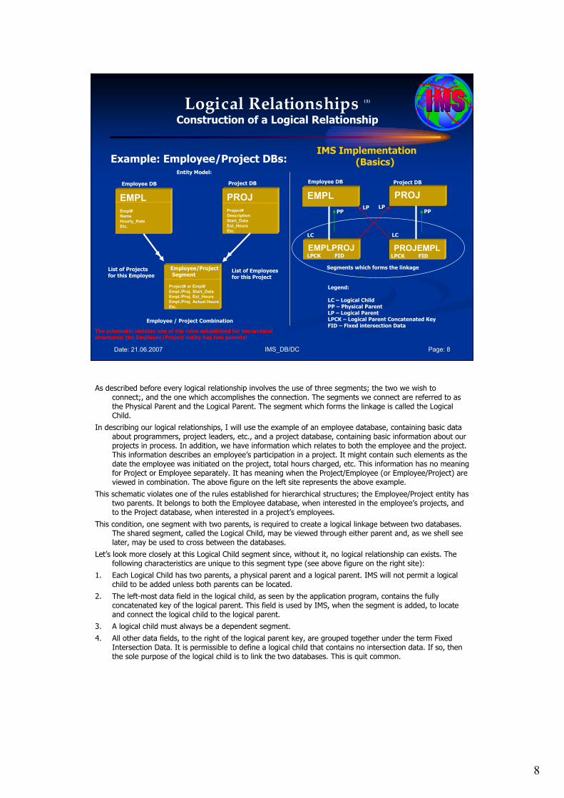
8
IMS_DB/DC Page: 8Date: 21.06.2007
Logical Relationships (3)
Construction of a Logical Relationship
Example: Employee/Project DBs:
EMPL
Empl#
Name
Hourly_Rate
Etc.
PROJ
Project#
Description
Start_Data
Est_Hours
Etc.
Employee DB Project DB
Project# or Empl#
Empl./Proj. Start_Data
Empl./Proj. Est_Hours
Empl./Proj. Actual Hours
Etc.
Employee/ProjectSegment
List of Projects for this Employee
List of Employees for this Project
Entity Model:
Employee / Project Combination
The schematic violates one of the rules established for hierarchical structures: the Employee/Project entity has two parents!
EMPL PROJ
EMPLPROJ PROJEMPL
LC LC
Employee DB Project DB
IMS Implementation(Basics)
Legend:
LC – Logical ChildPP – Physical ParentLP – Logical ParentLPCK – Logical Parent Concatenated KeyFID – Fixed intersection Data
Segments which forms the linkage
PP PPLP LP
LPCK FID LPCK FID
As described before every logical relationship involves the use of three segments; the two we wish to connect;, and the one which accomplishes the connection. The segments we connect are referred to as the Physical Parent and the Logical Parent. The segment which forms the linkage is called the Logical Child.
In describing our logical relationships, I will use the example of an employee database, containing basic data about programmers, project leaders, etc., and a project database, containing basic information about our projects in process. In addition, we have information which relates to both the employee and the project. This information describes an employee’s participation in a project. It might contain such elements as the date the employee was initiated on the project, total hours charged, etc. This information has no meaning for Project or Employee separately. It has meaning when the Project/Employee (or Employee/Project) are viewed in combination. The above figure on the left site represents the above example.
This schematic violates one of the rules established for hierarchical structures; the Employee/Project entity has two parents. It belongs to both the Employee database, when interested in the employee’s projects, and to the Project database, when interested in a project’s employees.
This condition, one segment with two parents, is required to create a logical linkage between two databases. The shared segment, called the Logical Child, may be viewed through either parent and, as we shell see later, may be used to cross between the databases.
Let’s look more closely at this Logical Child segment since, without it, no logical relationship can exists. The following characteristics are unique to this segment type (see above figure on the right site):
1. Each Logical Child has two parents, a physical parent and a logical parent. IMS will not permit a logical child to be added unless both parents can be located.
2. The left-most data field in the logical child, as seen by the application program, contains the fully concatenated key of the logical parent. This field is used by IMS, when the segment is added, to locate and connect the logical child to the logical parent.
3. A logical child must always be a dependent segment.
4. All other data fields, to the right of the logical parent key, are grouped together under the term Fixed Intersection Data. It is permissible to define a logical child that contains no intersection data. If so, then the sole purpose of the logical child is to link the two databases. This is quit common.
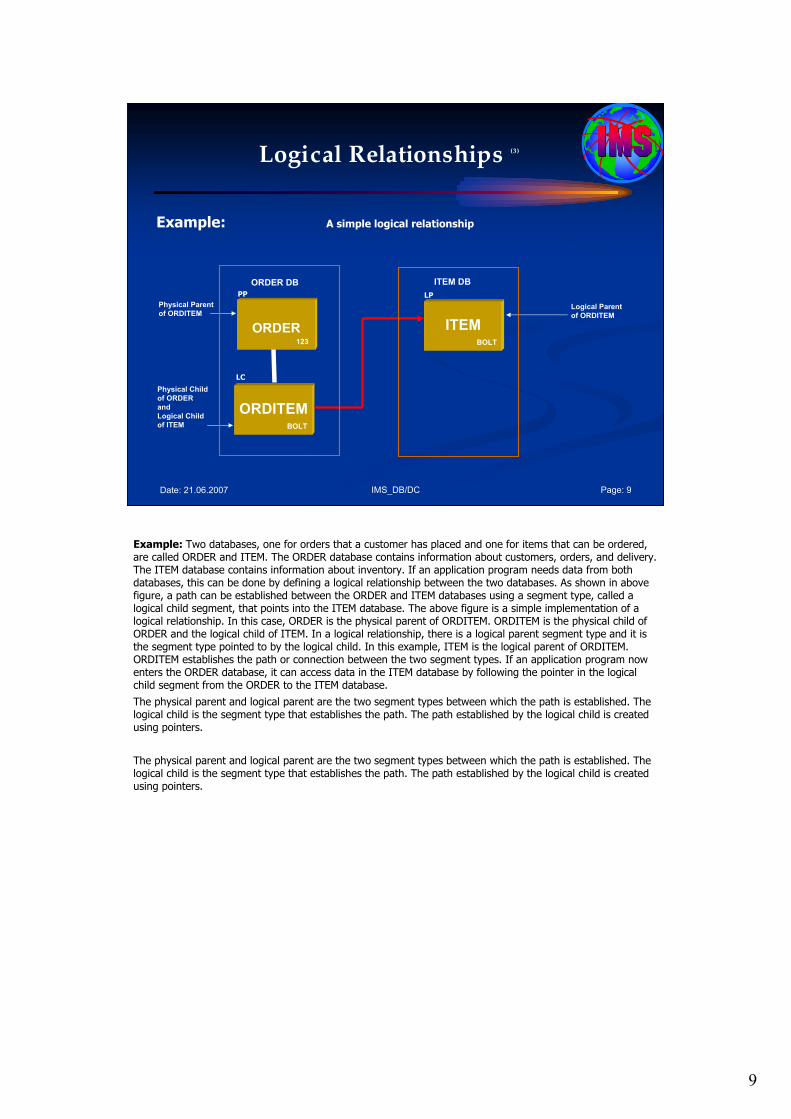
9
IMS_DB/DC Page: 9Date: 21.06.2007
Logical Relationships (3)
Example: A simple logical relationship
ORDITEM
ORDER123
Physical Parent
of ORDITEM
BOLT
ITEMBOLT
Physical Child
of ORDER
and
Logical Child
of ITEM
Logical Parent
of ORDITEM
ORDER DB ITEM DB
LC
PP LP
Example: Two databases, one for orders that a customer has placed and one for items that can be ordered, are called ORDER and ITEM. The ORDER database contains information about customers, orders, and delivery. The ITEM database contains information about inventory. If an application program needs data from both databases, this can be done by defining a logical relationship between the two databases. As shown in above figure, a path can be established between the ORDER and ITEM databases using a segment type, called a logical child segment, that points into the ITEM database. The above figure is a simple implementation of a logical relationship. In this case, ORDER is the physical parent of ORDITEM. ORDITEM is the physical child of ORDER and the logical child of ITEM. In a logical relationship, there is a logical parent segment type and it is the segment type pointed to by the logical child. In this example, ITEM is the logical parent of ORDITEM. ORDITEM establishes the path or connection between the two segment types. If an application program now enters the ORDER database, it can access data in the ITEM database by following the pointer in the logical child segment from the ORDER to the ITEM database.
The physical parent and logical parent are the two segment types between which the path is established. The logical child is the segment type that establishes the path. The path established by the logical child is created using pointers.
The physical parent and logical parent are the two segment types between which the path is established. The logical child is the segment type that establishes the path. The path established by the logical child is created using pointers.
10
IMS_DB/DC Page: 10Date: 21.06.2007
Agenda Session 4: Logical Relationships /Logical Databases
1. Logical Relationships
2. Implementation Methods• Unidirectional Relationship
• Bidirectional physically paired logical Relationships
• Bidirectional virtually paired logical Relationships
3. Paths in Logical Relationships
4. Logical Databases
5. Closing Comments
2. Implementation methods
11
IMS_DB/DC Page: 11Date: 21.06.2007
Implementation Methods (1)
Logical Relationship Types:
• Unidirectional logical relationships,
• Bidirectional physically paired logical relationships,
• Bidirectional virtually paired logical relationships.
Logical Relationship Types: Before you can design an efficient logical data structure, you must understand the three methods, which IMS has provided for implementing logical relationships.
Three types of logical relationships are discussed in this session:
•Unidirectional logical relationships,
•Bidirectional physically paired logical relationships,
•Bidirectional virtually paired logical relationships.
12
IMS_DB/DC Page: 12Date: 21.06.2007
Implementation Methods (2)
Logical Relationship Pointer Types:
The following topics look at pointing in logical relationships and the four types of pointers that you can specify for logical relationships:
• Logical Parent Pointer, • Logical Child Pointer, • Physical Parent Pointer, • Logical Twin Pointer.
For HALDBs, consider the following:
• Logical relationships are not allowed between HALDBs and non-HALDBs. • Direct pointers and indirect pointers are used. See “Indirect Pointers” later on.• Unidirectional relationships and bidirectional, physically paired relationships are supported for HALDBs. • Physical parent pointers are always present in PHDAM and PHIDAM segments.
Logical Relationship Pointer Types: In all logical relationships the logical child establishes a path between two segment types. The path is established by use of pointers. The following topics look at pointing in logical relationships and the four types of pointers that you can specify for logical relationships: •“Logical Parent Pointer”•“Logical Child Pointer”•“Physical Parent Pointer”•“Logical Twin Pointer”.For HALDBs, consider the following: •Logical relationships are not allowed between HALDBs and non-HALDBs. •Direct pointers and indirect pointers are used. See “Indirect Pointers” later on.•Unidirectional relationships and bidirectional, physically paired relationships are supported for HALDBs. •Physical parent pointers are always present in PHDAM and PHIDAM segments.
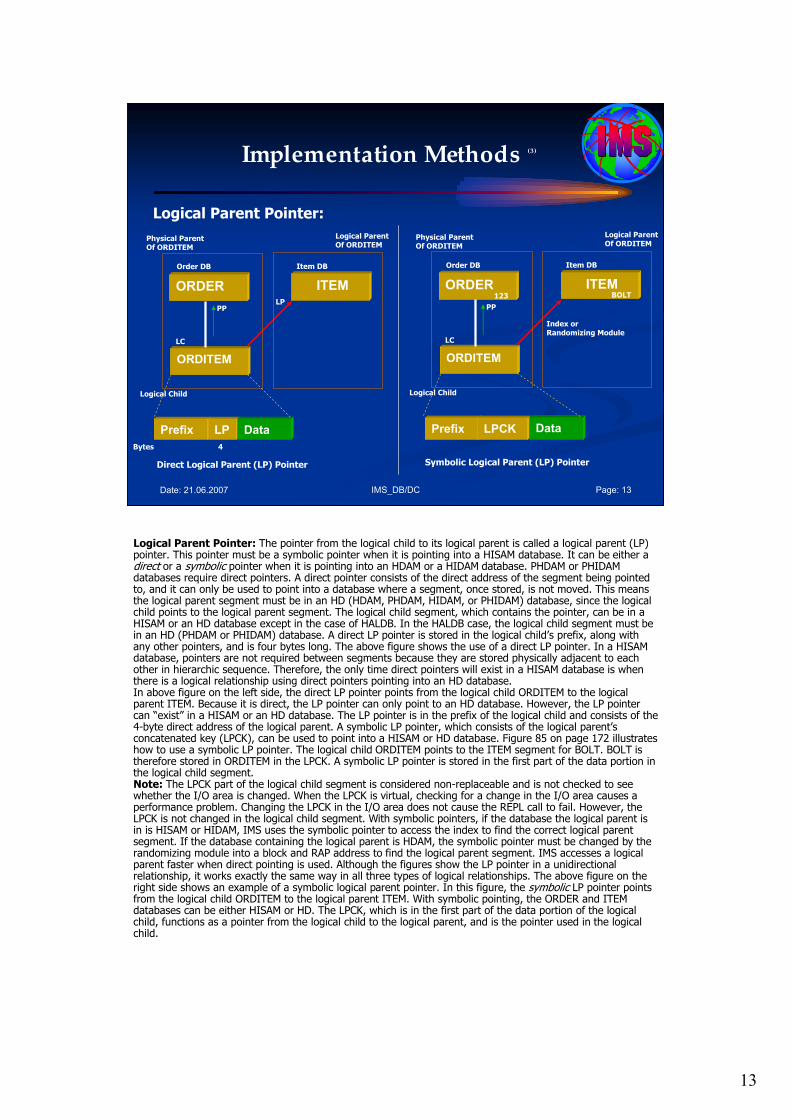
13
IMS_DB/DC Page: 13Date: 21.06.2007
Implementation Methods (3)
Logical Parent Pointer:
ORDER ITEM
ORDITEM
LC
Order DB Item DB
PPLP
Bytes 4
Prefix LP Data
Physical ParentOf ORDITEM
Logical Child
Logical ParentOf ORDITEM
Direct Logical Parent (LP) Pointer
ORDER ITEM
ORDITEM
LC
Order DB Item DB
PP
BOLT
Prefix LPCK Data
Physical ParentOf ORDITEM
Logical Child
Logical ParentOf ORDITEM
Symbolic Logical Parent (LP) Pointer
123
Index orRandomizing Module
Logical Parent Pointer: The pointer from the logical child to its logical parent is called a logical parent (LP) pointer. This pointer must be a symbolic pointer when it is pointing into a HISAM database. It can be either a direct or a symbolic pointer when it is pointing into an HDAM or a HIDAM database. PHDAM or PHIDAM databases require direct pointers. A direct pointer consists of the direct address of the segment being pointed to, and it can only be used to point into a database where a segment, once stored, is not moved. This means the logical parent segment must be in an HD (HDAM, PHDAM, HIDAM, or PHIDAM) database, since the logical child points to the logical parent segment. The logical child segment, which contains the pointer, can be in a HISAM or an HD database except in the case of HALDB. In the HALDB case, the logical child segment must be in an HD (PHDAM or PHIDAM) database. A direct LP pointer is stored in the logical child’s prefix, along with any other pointers, and is four bytes long. The above figure shows the use of a direct LP pointer. In a HISAM database, pointers are not required between segments because they are stored physically adjacent to each other in hierarchic sequence. Therefore, the only time direct pointers will exist in a HISAM database is when there is a logical relationship using direct pointers pointing into an HD database. In above figure on the left side, the direct LP pointer points from the logical child ORDITEM to the logical parent ITEM. Because it is direct, the LP pointer can only point to an HD database. However, the LP pointer can “exist” in a HISAM or an HD database. The LP pointer is in the prefix of the logical child and consists of the 4-byte direct address of the logical parent. A symbolic LP pointer, which consists of the logical parent’s concatenated key (LPCK), can be used to point into a HISAM or HD database. Figure 85 on page 172 illustrates how to use a symbolic LP pointer. The logical child ORDITEM points to the ITEM segment for BOLT. BOLT is therefore stored in ORDITEM in the LPCK. A symbolic LP pointer is stored in the first part of the data portion in the logical child segment. Note: The LPCK part of the logical child segment is considered non-replaceable and is not checked to see whether the I/O area is changed. When the LPCK is virtual, checking for a change in the I/O area causes a performance problem. Changing the LPCK in the I/O area does not cause the REPL call to fail. However, the LPCK is not changed in the logical child segment. With symbolic pointers, if the database the logical parent is in is HISAM or HIDAM, IMS uses the symbolic pointer to access the index to find the correct logical parent segment. If the database containing the logical parent is HDAM, the symbolic pointer must be changed by the randomizing module into a block and RAP address to find the logical parent segment. IMS accesses a logical parent faster when direct pointing is used. Although the figures show the LP pointer in a unidirectional relationship, it works exactly the same way in all three types of logical relationships. The above figure on the right side shows an example of a symbolic logical parent pointer. In this figure, the symbolic LP pointer points from the logical child ORDITEM to the logical parent ITEM. With symbolic pointing, the ORDER and ITEM databases can be either HISAM or HD. The LPCK, which is in the first part of the data portion of the logical child, functions as a pointer from the logical child to the logical parent, and is the pointer used in the logical child.
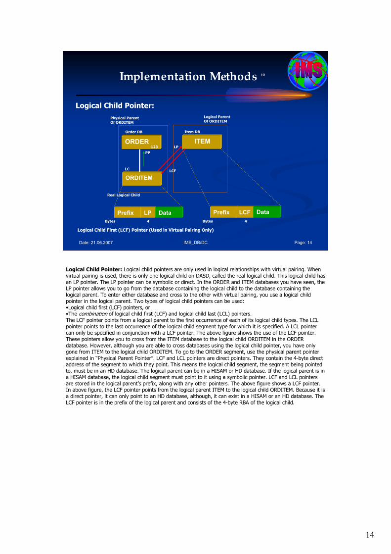
14
IMS_DB/DC Page: 14Date: 21.06.2007
Implementation Methods (4)
Logical Child Pointer:
ORDER ITEM
ORDITEM
LC
Order DB Item DB
PP
LP
Bytes 4
Prefix LP Data
Physical ParentOf ORDITEM
Real Logical Child
Logical ParentOf ORDITEM
Logical Child First (LCF) Pointer (Used in Virtual Pairing Only)
Prefix LCF Data
123
LCF
Bytes 4
Logical Child Pointer: Logical child pointers are only used in logical relationships with virtual pairing. When virtual pairing is used, there is only one logical child on DASD, called the real logical child. This logical child has an LP pointer. The LP pointer can be symbolic or direct. In the ORDER and ITEM databases you have seen, the LP pointer allows you to go from the database containing the logical child to the database containing the logical parent. To enter either database and cross to the other with virtual pairing, you use a logical child pointer in the logical parent. Two types of logical child pointers can be used: •Logical child first (LCF) pointers, or •The combination of logical child first (LCF) and logical child last (LCL) pointers.The LCF pointer points from a logical parent to the first occurrence of each of its logical child types. The LCL pointer points to the last occurrence of the logical child segment type for which it is specified. A LCL pointer can only be specified in conjunction with a LCF pointer. The above figure shows the use of the LCF pointer. These pointers allow you to cross from the ITEM database to the logical child ORDITEM in the ORDER database. However, although you are able to cross databases using the logical child pointer, you have only gone from ITEM to the logical child ORDITEM. To go to the ORDER segment, use the physical parent pointer explained in “Physical Parent Pointer”. LCF and LCL pointers are direct pointers. They contain the 4-byte direct address of the segment to which they point. This means the logical child segment, the segment being pointed to, must be in an HD database. The logical parent can be in a HISAM or HD database. If the logical parent is in a HISAM database, the logical child segment must point to it using a symbolic pointer. LCF and LCL pointers are stored in the logical parent’s prefix, along with any other pointers. The above figure shows a LCF pointer. In above figure, the LCF pointer points from the logical parent ITEM to the logical child ORDITEM. Because it is a direct pointer, it can only point to an HD database, although, it can exist in a HISAM or an HD database. The LCF pointer is in the prefix of the logical parent and consists of the 4-byte RBA of the logical child.
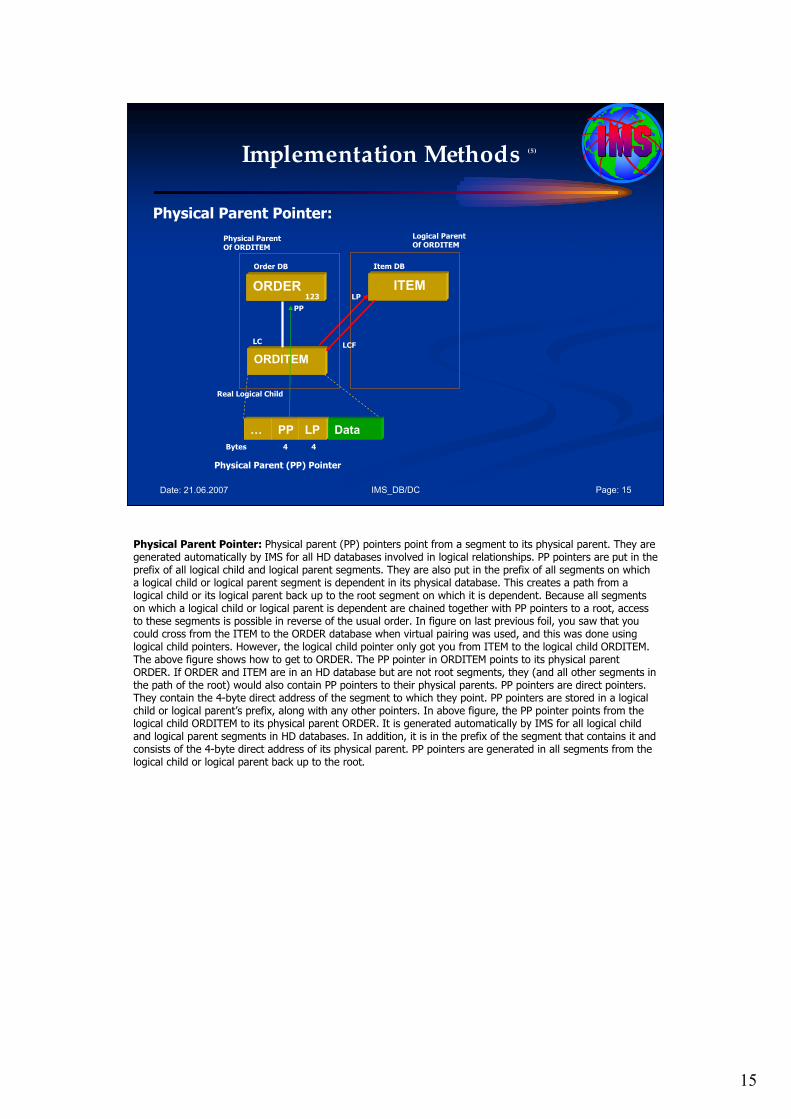
15
IMS_DB/DC Page: 15Date: 21.06.2007
Implementation Methods (5)
Physical Parent Pointer:
ORDER ITEM
ORDITEM
LC
Order DB Item DB
PP
LP
Bytes 4 4
…
Physical ParentOf ORDITEM
Real Logical Child
Logical ParentOf ORDITEM
Physical Parent (PP) Pointer
123
LCF
PP LP Data
Physical Parent Pointer: Physical parent (PP) pointers point from a segment to its physical parent. They are generated automatically by IMS for all HD databases involved in logical relationships. PP pointers are put in the prefix of all logical child and logical parent segments. They are also put in the prefix of all segments on which a logical child or logical parent segment is dependent in its physical database. This creates a path from a logical child or its logical parent back up to the root segment on which it is dependent. Because all segments on which a logical child or logical parent is dependent are chained together with PP pointers to a root, access to these segments is possible in reverse of the usual order. In figure on last previous foil, you saw that you could cross from the ITEM to the ORDER database when virtual pairing was used, and this was done using logical child pointers. However, the logical child pointer only got you from ITEM to the logical child ORDITEM. The above figure shows how to get to ORDER. The PP pointer in ORDITEM points to its physical parent ORDER. If ORDER and ITEM are in an HD database but are not root segments, they (and all other segments in the path of the root) would also contain PP pointers to their physical parents. PP pointers are direct pointers. They contain the 4-byte direct address of the segment to which they point. PP pointers are stored in a logical child or logical parent’s prefix, along with any other pointers. In above figure, the PP pointer points from the logical child ORDITEM to its physical parent ORDER. It is generated automatically by IMS for all logical child and logical parent segments in HD databases. In addition, it is in the prefix of the segment that contains it and consists of the 4-byte direct address of its physical parent. PP pointers are generated in all segments from the logical child or logical parent back up to the root.
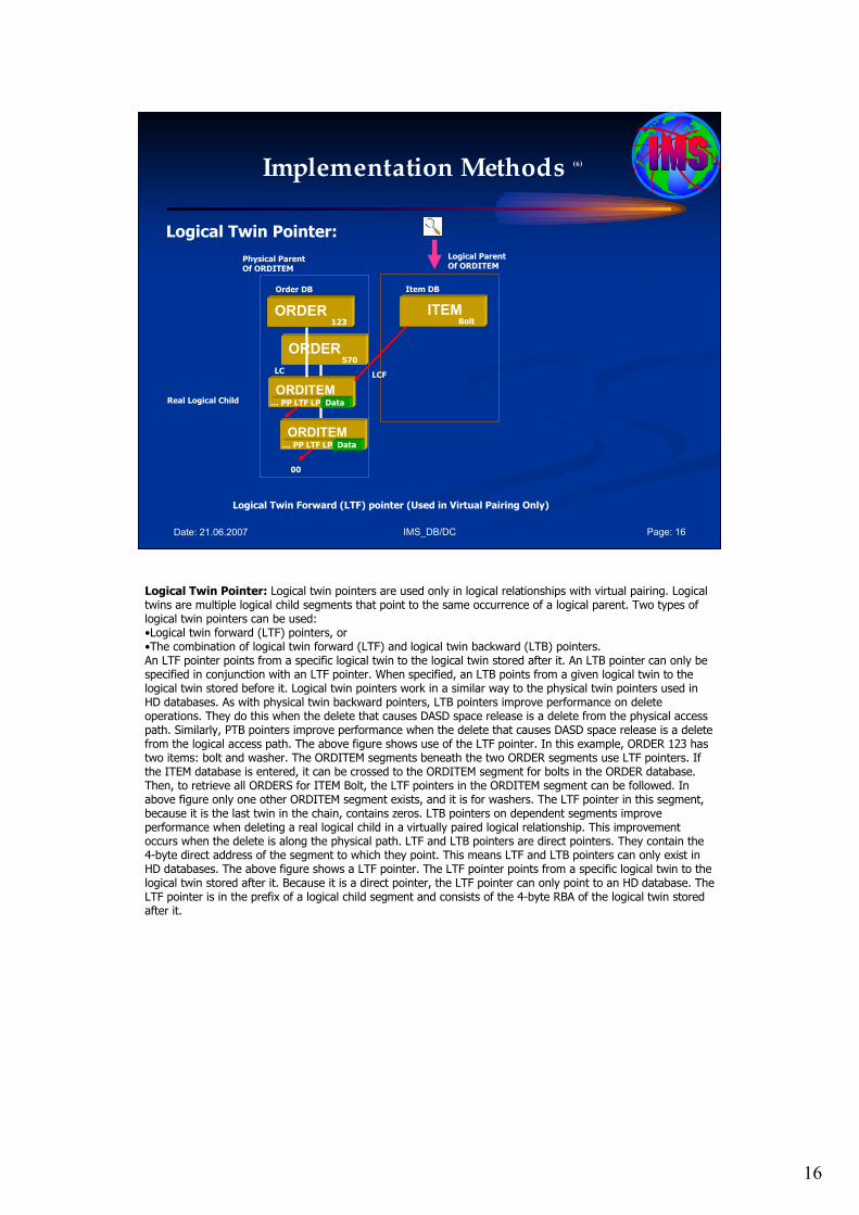
16
IMS_DB/DC Page: 16Date: 21.06.2007
Implementation Methods (6)
Logical Twin Pointer:
ORDER
ORDER ITEM
ORDITEM
LC
Order DB Item DB
Physical ParentOf ORDITEM
Real Logical Child
Logical ParentOf ORDITEM
Logical Twin Forward (LTF) pointer (Used in Virtual Pairing Only)
123
LCF
Bolt
… PP LTF LP Data
ORDITEM… PP LTF LP Data
00
570
Logical Twin Pointer: Logical twin pointers are used only in logical relationships with virtual pairing. Logical twins are multiple logical child segments that point to the same occurrence of a logical parent. Two types of logical twin pointers can be used: •Logical twin forward (LTF) pointers, or •The combination of logical twin forward (LTF) and logical twin backward (LTB) pointers. An LTF pointer points from a specific logical twin to the logical twin stored after it. An LTB pointer can only be specified in conjunction with an LTF pointer. When specified, an LTB points from a given logical twin to the logical twin stored before it. Logical twin pointers work in a similar way to the physical twin pointers used in HD databases. As with physical twin backward pointers, LTB pointers improve performance on delete operations. They do this when the delete that causes DASD space release is a delete from the physical access path. Similarly, PTB pointers improve performance when the delete that causes DASD space release is a delete from the logical access path. The above figure shows use of the LTF pointer. In this example, ORDER 123 has two items: bolt and washer. The ORDITEM segments beneath the two ORDER segments use LTF pointers. If the ITEM database is entered, it can be crossed to the ORDITEM segment for bolts in the ORDER database. Then, to retrieve all ORDERS for ITEM Bolt, the LTF pointers in the ORDITEM segment can be followed. In above figure only one other ORDITEM segment exists, and it is for washers. The LTF pointer in this segment, because it is the last twin in the chain, contains zeros. LTB pointers on dependent segments improve performance when deleting a real logical child in a virtually paired logical relationship. This improvement occurs when the delete is along the physical path. LTF and LTB pointers are direct pointers. They contain the 4-byte direct address of the segment to which they point. This means LTF and LTB pointers can only exist in HD databases. The above figure shows a LTF pointer. The LTF pointer points from a specific logical twin to the logical twin stored after it. Because it is a direct pointer, the LTF pointer can only point to an HD database. The LTF pointer is in the prefix of a logical child segment and consists of the 4-byte RBA of the logical twin stored after it.
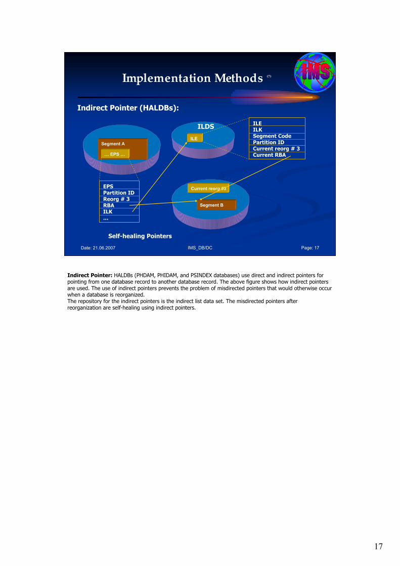
17
IMS_DB/DC Page: 17Date: 21.06.2007
Implementation Methods (7)
Indirect Pointer (HALDBs):
Segment A
… EPS …
Self-healing Pointers
ILE
Current reorg #3
Segment B
ILDS
EPSPartition IDReorg # 3RBAILK…
ILEILKSegment CodePartition IDCurrent reorg # 3Current RBA
Indirect Pointer: HALDBs (PHDAM, PHIDAM, and PSINDEX databases) use direct and indirect pointers for pointing from one database record to another database record. The above figure shows how indirect pointers are used. The use of indirect pointers prevents the problem of misdirected pointers that would otherwise occur when a database is reorganized. The repository for the indirect pointers is the indirect list data set. The misdirected pointers after reorganization are self-healing using indirect pointers.
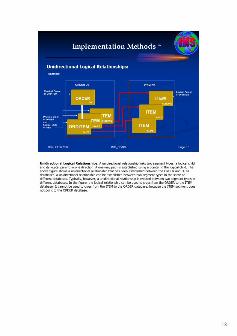
18
IMS_DB/DC Page: 18Date: 21.06.2007
Implementation Methods (8)
Unidirectional Logical Relationships:
ORDITEMORDITEM
ITEM
ITEM
ORDITEM
ORDER578
Physical Parent
of ORDITEM
CLIPS
ITEM
SCREWS
Physical Child
of ORDER
and
Logical Child
of ITEM
Logical Parent
of ORDITEM
ORDER DB ITEM DB
NAILS
SCREWS
CLIPS
NAILS
Example:
Unidirectional Logical Relationships: A unidirectional relationship links two segment types, a logical child and its logical parent, in one direction. A one-way path is established using a pointer in the logical child. The above figure shows a unidirectional relationship that has been established between the ORDER and ITEM databases. A unidirectional relationship can be established between two segment types in the same or different databases. Typically, however, a unidirectional relationship is created between two segment types in different databases. In the figure, the logical relationship can be used to cross from the ORDER to the ITEM database. It cannot be used to cross from the ITEM to the ORDER database, because the ITEM segment does not point to the ORDER database.
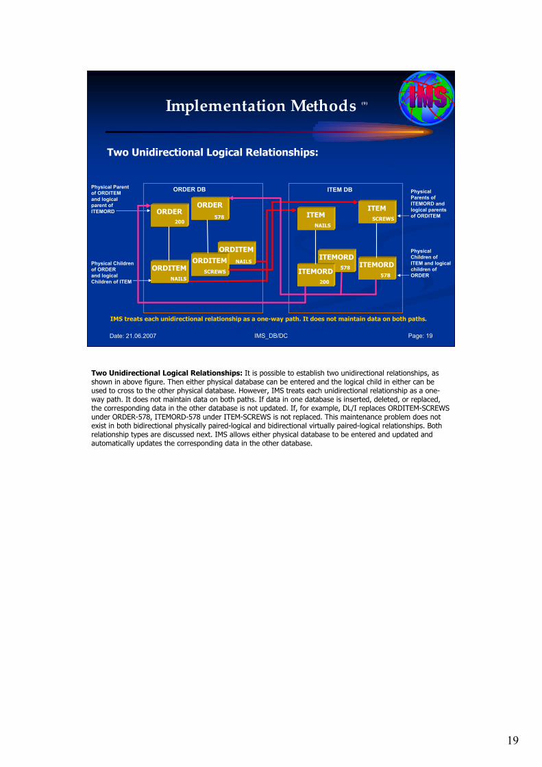
19
IMS_DB/DC Page: 19Date: 21.06.2007
Implementation Methods (9)
Two Unidirectional Logical Relationships:
ITEMORDORDITEM
ORDITEM
SCREWS
ORDER
578ORDER
Physical Parent
of ORDITEM
and logical
parent of
ITEMORD
Physical Children
of ORDER
and logical
Children of ITEM
Physical
Parents of
ITEMORD and
logical parents
of ORDITEM
ORDER DB ITEM DB
ORDITEM
NAILS
NAILS
ITEM
ITEMORD
NAILS
200
578
ITEM
ITEMORD
SCREWS
578
200
Physical
Children of
ITEM and logical
children of
ORDER
IMS treats each unidirectional relationship as a one-way path. It does not maintain data on both paths.
Two Unidirectional Logical Relationships: It is possible to establish two unidirectional relationships, as shown in above figure. Then either physical database can be entered and the logical child in either can be used to cross to the other physical database. However, IMS treats each unidirectional relationship as a one-way path. It does not maintain data on both paths. If data in one database is inserted, deleted, or replaced, the corresponding data in the other database is not updated. If, for example, DL/I replaces ORDITEM-SCREWS under ORDER-578, ITEMORD-578 under ITEM-SCREWS is not replaced. This maintenance problem does not exist in both bidirectional physically paired-logical and bidirectional virtually paired-logical relationships. Both relationship types are discussed next. IMS allows either physical database to be entered and updated and automatically updates the corresponding data in the other database.

20
IMS_DB/DC Page: 20Date: 21.06.2007
Implementation Methods (10)
IMS Unidirectional Logical Relationship (UR):
EMPL
EMPLPROJ
PROJ
LPPP
LC
Example:
• LP pointer (optional when LP is defined in HDAM or HIDAM,• through symbolic pointer with Option “P” in parent-parameter (required when LP is in HISAM),• through LP pointer and symbolic pointer.
A
B
C
LPPP
LC
IMS Schema
IMS Unidirectional Logical Relationship (UR): This implementation method builds a linkage between the Logical Child and its logical Parent in only one direction. The logical Child is not accessible from the logical Parent. The only purpose of this method is to build a direct link from the LC to the LP so that we can efficiently cross between the databases in that one direction as shown in above figure.
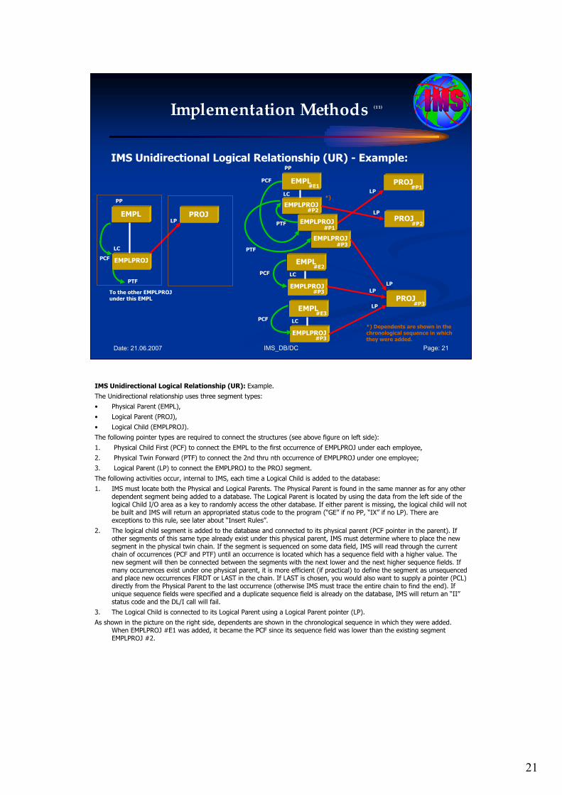
21
IMS_DB/DC Page: 21Date: 21.06.2007
Implementation Methods (11)
IMS Unidirectional Logical Relationship (UR) - Example:
EMPL
EMPLPROJ
PROJLP
PP
LC
PCF
EMPLPROJ
EMPLPROJ
#P2
#P1
#P3
#P1
PROJ#P2
PROJ#P3
#E1
LP
LP
EMPL
EMPLPROJ
LC
#P3
#E2
EMPL
EMPLPROJ
LC
#P3
#E3
LP
LP
PTF
PTF
PCF
PCF
*)
*) Dependents are shown in the chronological sequence in which they were added.
EMPL
EMPLPROJ
PROJLP
PP
LC
PCF
PTF
To the other EMPLPROJ under this EMPL
IMS Unidirectional Logical Relationship (UR): Example.
The Unidirectional relationship uses three segment types:
• Physical Parent (EMPL),
• Logical Parent (PROJ),
• Logical Child (EMPLPROJ).
The following pointer types are required to connect the structures (see above figure on left side):
1. Physical Child First (PCF) to connect the EMPL to the first occurrence of EMPLPROJ under each employee,
2. Physical Twin Forward (PTF) to connect the 2nd thru nth occurrence of EMPLPROJ under one employee;
3. Logical Parent (LP) to connect the EMPLPROJ to the PROJ segment.
The following activities occur, internal to IMS, each time a Logical Child is added to the database:
1. IMS must locate both the Physical and Logical Parents. The Physical Parent is found in the same manner as for any other dependent segment being added to a database. The Logical Parent is located by using the data from the left side of the logical Child I/O area as a key to randomly access the other database. If either parent is missing, the logical child will not be built and IMS will return an appropriated status code to the program (“GE” if no PP, “IX” if no LP). There are exceptions to this rule, see later about “Insert Rules”.
2. The logical child segment is added to the database and connected to its physical parent (PCF pointer in the parent). If other segments of this same type already exist under this physical parent, IMS must determine where to place the new segment in the physical twin chain. If the segment is sequenced on some data field, IMS will read through the current chain of occurrences (PCF and PTF) until an occurrence is located which has a sequence field with a higher value. The new segment will then be connected between the segments with the next lower and the next higher sequence fields. If many occurrences exist under one physical parent, it is more efficient (if practical) to define the segment as unsequencedand place new occurrences FIRDT or LAST in the chain. If LAST is chosen, you would also want to supply a pointer (PCL) directly from the Physical Parent to the last occurrence (otherwise IMS must trace the entire chain to find the end). If unique sequence fields were specified and a duplicate sequence field is already on the database, IMS will return an “II”status code and the DL/I call will fail.
3. The Logical Child is connected to its Logical Parent using a Logical Parent pointer (LP).
As shown in the picture on the right side, dependents are shown in the chronological sequence in which they were added. When EMPLPROJ #E1 was added, it became the PCF since its sequence field was lower than the existing segment EMPLPROJ #2.
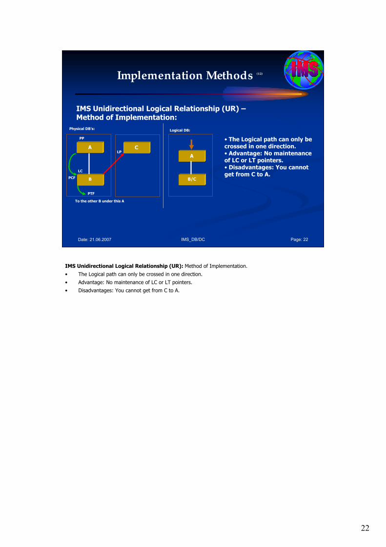
22
IMS_DB/DC Page: 22Date: 21.06.2007
Implementation Methods (12)
IMS Unidirectional Logical Relationship (UR) –Method of Implementation:
A
B
CLP
PP
LC
PCF
PTF
To the other B under this A
Physical DB’s:
A
B/C
Logical DB:
• The Logical path can only be crossed in one direction.• Advantage: No maintenance of LC or LT pointers.• Disadvantages: You cannot get from C to A.
IMS Unidirectional Logical Relationship (UR): Method of Implementation.
• The Logical path can only be crossed in one direction.
• Advantage: No maintenance of LC or LT pointers.
• Disadvantages: You cannot get from C to A.
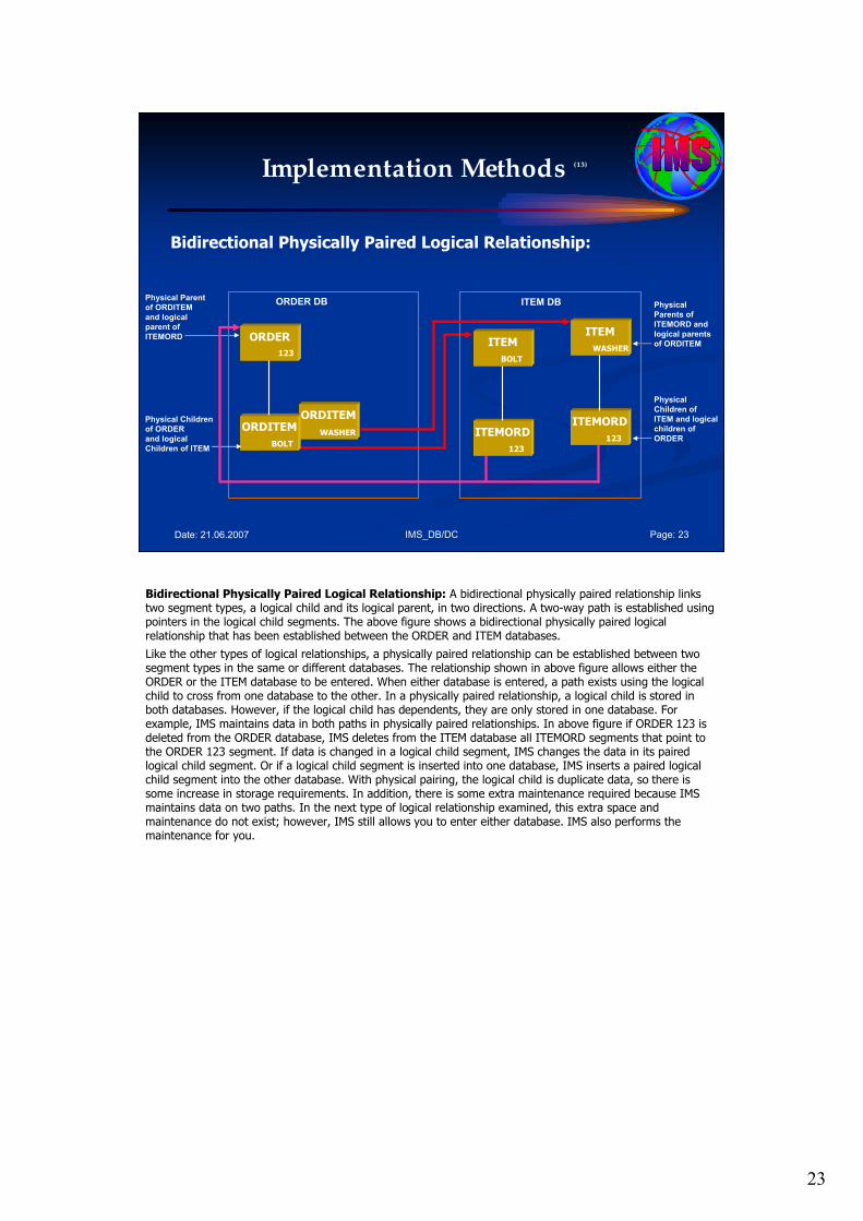
23
IMS_DB/DC Page: 23Date: 21.06.2007
Implementation Methods (13)
Bidirectional Physically Paired Logical Relationship:
ORDITEM
WASHER
ORDER
Physical Parent
of ORDITEM
and logical
parent of
ITEMORD
Physical Children
of ORDER
and logical
Children of ITEM
Physical
Parents of
ITEMORD and
logical parents
of ORDITEM
ORDER DB ITEM DB
ORDITEM
BOLT
ITEM
ITEMORD
BOLT
123
ITEM
ITEMORD
WASHER
123
123
Physical
Children of
ITEM and logical
children of
ORDER
Bidirectional Physically Paired Logical Relationship: A bidirectional physically paired relationship links two segment types, a logical child and its logical parent, in two directions. A two-way path is established using pointers in the logical child segments. The above figure shows a bidirectional physically paired logical relationship that has been established between the ORDER and ITEM databases.
Like the other types of logical relationships, a physically paired relationship can be established between two segment types in the same or different databases. The relationship shown in above figure allows either the ORDER or the ITEM database to be entered. When either database is entered, a path exists using the logical child to cross from one database to the other. In a physically paired relationship, a logical child is stored in both databases. However, if the logical child has dependents, they are only stored in one database. For example, IMS maintains data in both paths in physically paired relationships. In above figure if ORDER 123 is deleted from the ORDER database, IMS deletes from the ITEM database all ITEMORD segments that point to the ORDER 123 segment. If data is changed in a logical child segment, IMS changes the data in its paired logical child segment. Or if a logical child segment is inserted into one database, IMS inserts a paired logical child segment into the other database. With physical pairing, the logical child is duplicate data, so there is some increase in storage requirements. In addition, there is some extra maintenance required because IMS maintains data on two paths. In the next type of logical relationship examined, this extra space and maintenance do not exist; however, IMS still allows you to enter either database. IMS also performs the maintenance for you.
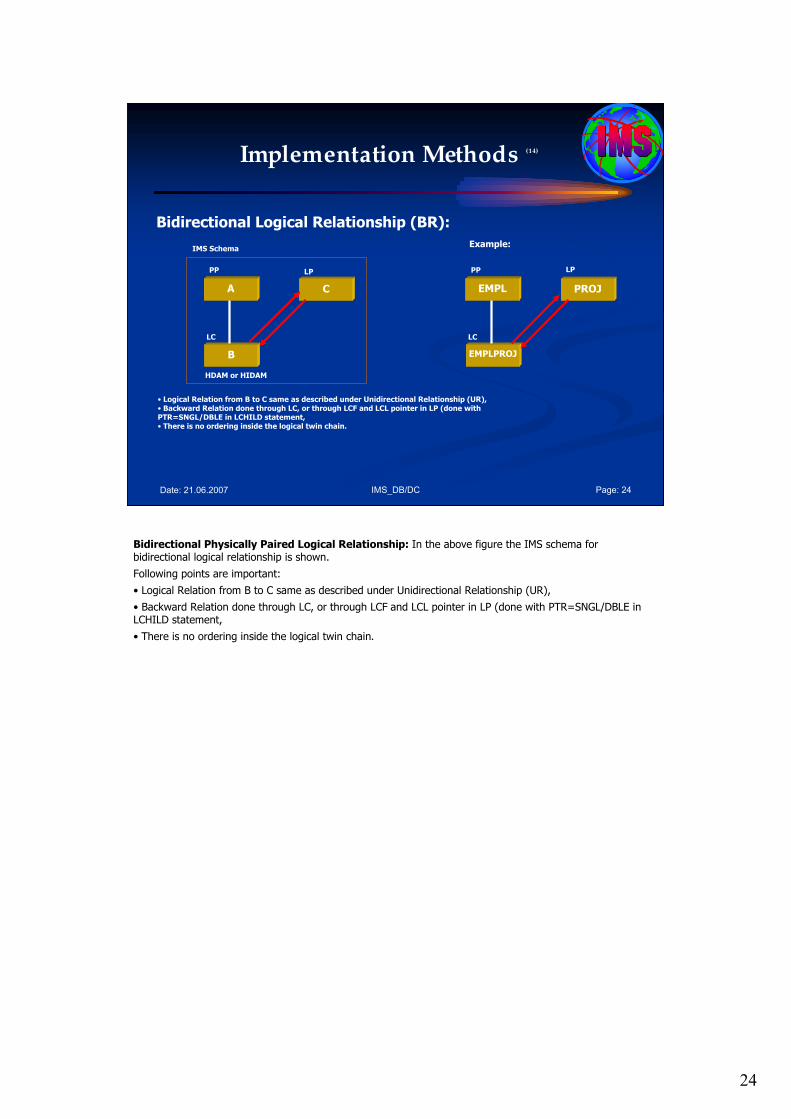
24
IMS_DB/DC Page: 24Date: 21.06.2007
Implementation Methods (14)
Bidirectional Logical Relationship (BR):
• Logical Relation from B to C same as described under Unidirectional Relationship (UR),• Backward Relation done through LC, or through LCF and LCL pointer in LP (done with PTR=SNGL/DBLE in LCHILD statement,• There is no ordering inside the logical twin chain.
A
B
C
LPPP
LC
IMS Schema
HDAM or HIDAM
EMPL
EMPLPROJ
PROJ
LPPP
LC
Example:
Bidirectional Physically Paired Logical Relationship: In the above figure the IMS schema for bidirectional logical relationship is shown.
Following points are important:
• Logical Relation from B to C same as described under Unidirectional Relationship (UR),
• Backward Relation done through LC, or through LCF and LCL pointer in LP (done with PTR=SNGL/DBLE in LCHILD statement,
• There is no ordering inside the logical twin chain.
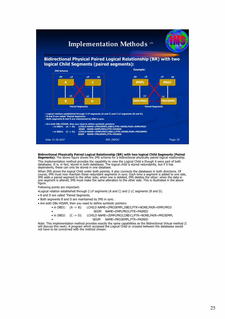
25
IMS_DB/DC Page: 25Date: 21.06.2007
Implementation Methods (15)
Bidirectional Physical Paired Logical Relationship (BR) with twological Child Segments (paired segments):
• Logical relation established through 2 LP segments (A and C) and 2 LC segments (B and D).• B and D are called “Paired Segments.• Both segments B and D are maintained by IMS in sync.
• Are both DBs HISAM, then you need to define symbolic pointers:• in DBD1: (A -> B): LCHILD NAME=(PROJEMPL,DBD2,PTR=NONE,PAIR=EMPLPROJ
SEGM NAME=EMPLPROJ,PTR=PAIRED• in DBD2: (C -> D): LCHILD NAME=(EMPLPROJ,DBD1),PTR=NONE,PAIR=PROJEMPL
SEGM NAME=PROJEMPL,PTR=PAIRED
A
B
C
LPPP
LC
IMS Schema
D
LC
LP PP
Paired Segments
EMPL
EMPLPROJ
PROJ
LPPP
LC
Example:
PROJEMPL
LC
LP PP
Paired Segments
Bidirectional Physically Paired Logical Relationship (BR) with two logical Child Segments (Paired Segments): The above figure shows the IMS schema for a bidirectional physically paired logical relationship.
This implementation method provides the capability to view the Logical Child a though it were part of both databases. It is, in fact, stored in both databases. The logical child is stored redundantly, but if it has dependents, these can only be stored in one database.
When IMS stores the logical Child under both parents, it also connects the databases in both directions. Of course, IMS must now maintain these redundant segments in sync. Each time a segment is added to one side, IMS adds a paired segment to the other side; when one is deleted, IMS deletes the other; when the data in one segment is altered, IMS must make the same alteration to the other side. This is illustrated in the above figure.
Following points are important:
•Logical relation established through 2 LP segments (A and C) and 2 LC segments (B and D).
• B and D are called “Paired Segments.
• Both segments B and D are maintained by IMS in sync.
• Are both DBs HISAM, then you need to define symbolic pointers:
• in DBD1: (A -> B): LCHILD NAME=(PROJEMPL,DBD2,PTR=NONE,PAIR=EMPLPROJ
• SEGM NAME=EMPLPROJ,PTR=PAIRED
• in DBD2: (C -> D): LCHILD NAME=(EMPLPROJ,DBD1),PTR=NONE,PAIR=PROJEMPL
• SEGM NAME=PROJEMPL,PTR=PAIRED
Note: This implementation method provides exactly the same capabilities as the Bidirectional Virtual method (I will discuss this next). A program which accessed the Logical Child or crossed between the databases would not have to be concerned with the method chosen.
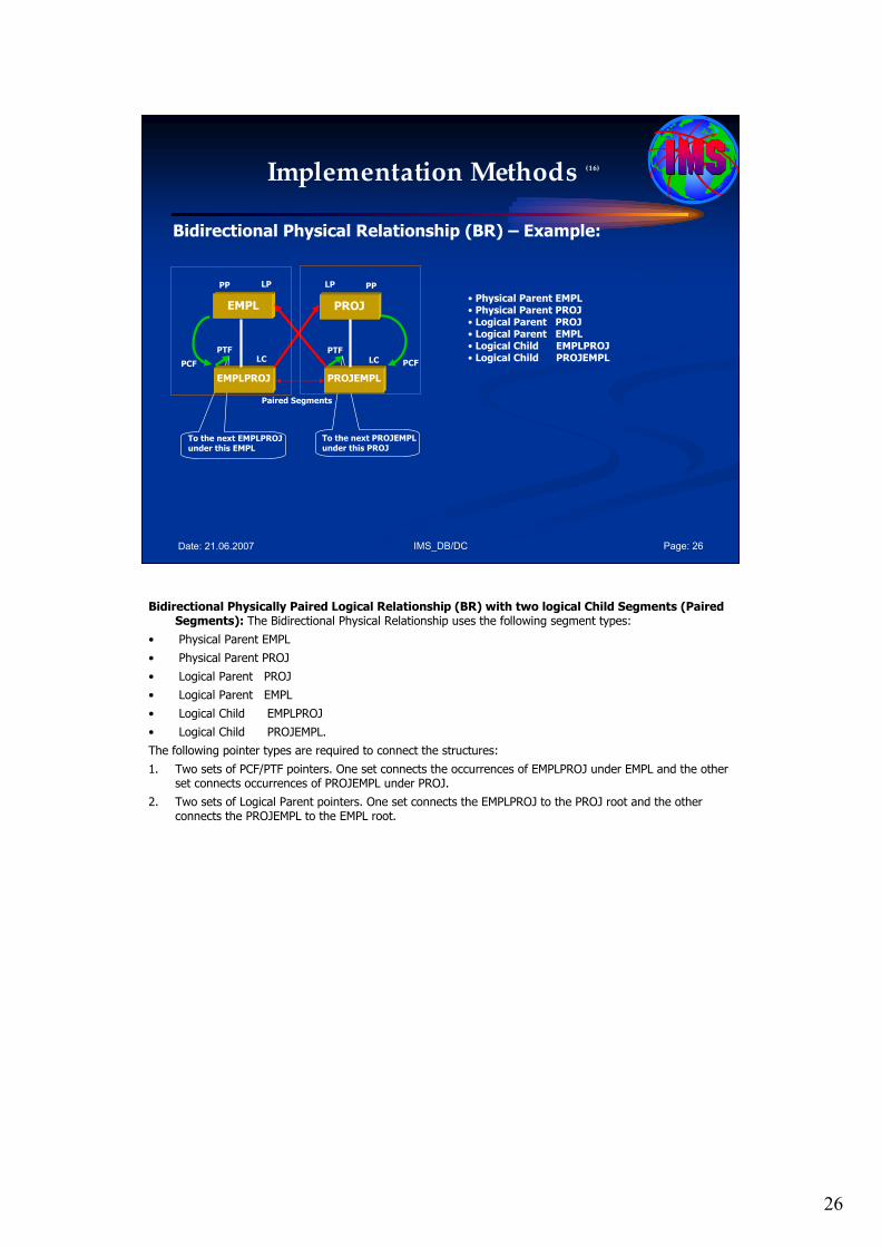
26
IMS_DB/DC Page: 26Date: 21.06.2007
Implementation Methods (16)
Bidirectional Physical Relationship (BR) – Example:
To the next EMPLPROJ under this EMPL
To the next PROJEMPL under this PROJ
• Physical Parent EMPL• Physical Parent PROJ• Logical Parent PROJ• Logical Parent EMPL• Logical Child EMPLPROJ• Logical Child PROJEMPL
PCF
EMPL
EMPLPROJ
PROJ
LPPP
LC
PROJEMPL
LC
LP PP
Paired Segments
PCF
PTF PTF
Bidirectional Physically Paired Logical Relationship (BR) with two logical Child Segments (Paired Segments): The Bidirectional Physical Relationship uses the following segment types:
• Physical Parent EMPL
• Physical Parent PROJ
• Logical Parent PROJ
• Logical Parent EMPL
• Logical Child EMPLPROJ
• Logical Child PROJEMPL.
The following pointer types are required to connect the structures:
1. Two sets of PCF/PTF pointers. One set connects the occurrences of EMPLPROJ under EMPL and the other set connects occurrences of PROJEMPL under PROJ.
2. Two sets of Logical Parent pointers. One set connects the EMPLPROJ to the PROJ root and the other connects the PROJEMPL to the EMPL root.
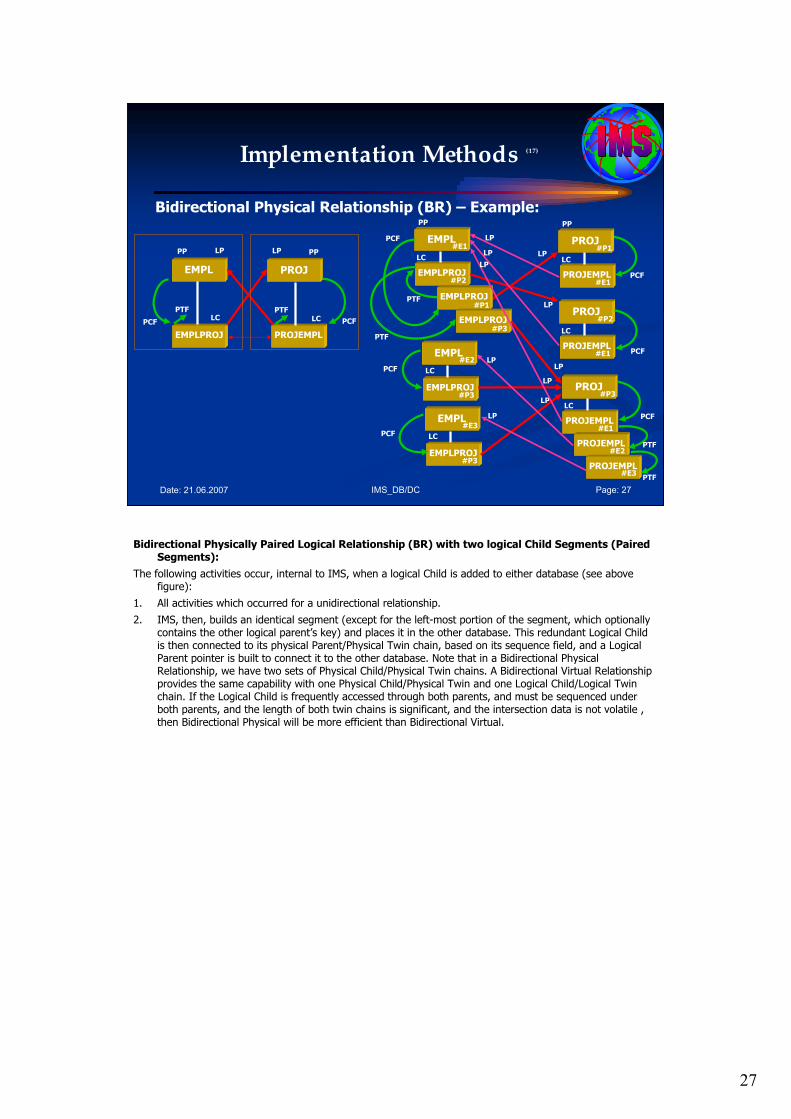
27
IMS_DB/DC Page: 27Date: 21.06.2007
Implementation Methods (17)
Bidirectional Physical Relationship (BR) – Example:
EMPL
EMPLPROJ
PROJ
LPPP
LC
PROJEMPL
LC
LP PP
PCF PCF
PTF PTF
EMPL
EMPLPROJ
PROJLP
PP
LC
PCF
EMPLPROJ
EMPLPROJ
#P2
#P1
#P3
#P1
PROJ#P2
PROJ#P3
#E1
LP
LP
EMPL
EMPLPROJ
LC
#P3
#E2
EMPL
EMPLPROJ
LC
#P3
#E3
LP
LP
PTF
PTF
PCF
PCF
PROJEMPL
LC
#E1
PROJEMPL
LC
#E1
PROJEMPL
LC
#E1
PROJEMPL#E2
PROJEMPL#E3
PCF
PCF
PCF
PTF
PTF
LP
LP
LP
LP
LP
PP
Bidirectional Physically Paired Logical Relationship (BR) with two logical Child Segments (Paired Segments):
The following activities occur, internal to IMS, when a logical Child is added to either database (see above figure):
1. All activities which occurred for a unidirectional relationship.
2. IMS, then, builds an identical segment (except for the left-most portion of the segment, which optionally contains the other logical parent’s key) and places it in the other database. This redundant Logical Child is then connected to its physical Parent/Physical Twin chain, based on its sequence field, and a Logical Parent pointer is built to connect it to the other database. Note that in a Bidirectional Physical Relationship, we have two sets of Physical Child/Physical Twin chains. A Bidirectional Virtual Relationship provides the same capability with one Physical Child/Physical Twin and one Logical Child/Logical Twin chain. If the Logical Child is frequently accessed through both parents, and must be sequenced under both parents, and the length of both twin chains is significant, and the intersection data is not volatile , then Bidirectional Physical will be more efficient than Bidirectional Virtual.
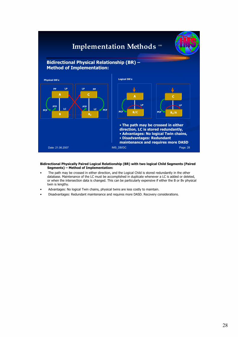
28
IMS_DB/DC Page: 28Date: 21.06.2007
Implementation Methods (18)
Bidirectional Physical Relationship (BR) –Method of Implementation:
A
B
C
LPPP
LC
BV
LC
LP PP
PCF PCF
PTF PTF
Physical DB’s: Logical DB’s:
A
B/CPCF
LP
C
BV/APCF
LP
• The path may be crossed in either direction, LC is stored redundantly,• Advantages: No logical Twin chains,• Disadvantages: Redundant maintenance and requires more DASD
Bidirectional Physically Paired Logical Relationship (BR) with two logical Child Segments (Paired Segments) – Method of Implementation:
• The path may be crossed in either direction, and the Logical Child is stored redundantly in the other database. Maintenance of the LC must be accomplished in duplicate whenever a LC is added or deleted, or when the intersection data is changed. This can be particularly expensive if either the B or Bv physical twin is lengthy.
• Advantages: No logical Twin chains, physical twins are less costly to maintain.
• Disadvantages: Redundant maintenance and requires more DASD. Recovery considerations.
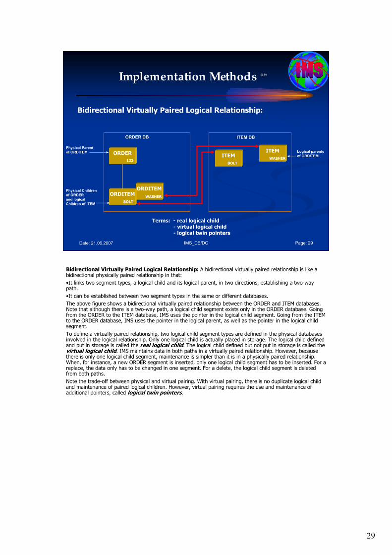
29
IMS_DB/DC Page: 29Date: 21.06.2007
Implementation Methods (19)
Bidirectional Virtually Paired Logical Relationship:
ORDITEM
WASHER
ORDERPhysical Parent
of ORDITEM
Physical Children
of ORDER
and logical
Children of ITEM
Logical parents
of ORDITEM
ORDER DB ITEM DB
ORDITEM
BOLT
ITEM
BOLT
ITEM
WASHER123
Terms: - real logical child- virtual logical child- logical twin pointers
Bidirectional Virtually Paired Logical Relationship: A bidirectional virtually paired relationship is like a bidirectional physically paired relationship in that:
•It links two segment types, a logical child and its logical parent, in two directions, establishing a two-way path.
•It can be established between two segment types in the same or different databases.
The above figure shows a bidirectional virtually paired relationship between the ORDER and ITEM databases. Note that although there is a two-way path, a logical child segment exists only in the ORDER database. Going from the ORDER to the ITEM database, IMS uses the pointer in the logical child segment. Going from the ITEM to the ORDER database, IMS uses the pointer in the logical parent, as well as the pointer in the logical child segment.
To define a virtually paired relationship, two logical child segment types are defined in the physical databases involved in the logical relationship. Only one logical child is actually placed in storage. The logical child defined and put in storage is called the real logical child. The logical child defined but not put in storage is called thevirtual logical child. IMS maintains data in both paths in a virtually paired relationship. However, because there is only one logical child segment, maintenance is simpler than it is in a physically paired relationship. When, for instance, a new ORDER segment is inserted, only one logical child segment has to be inserted. For a replace, the data only has to be changed in one segment. For a delete, the logical child segment is deleted from both paths.
Note the trade-off between physical and virtual pairing. With virtual pairing, there is no duplicate logical child and maintenance of paired logical children. However, virtual pairing requires the use and maintenance of additional pointers, called logical twin pointers.
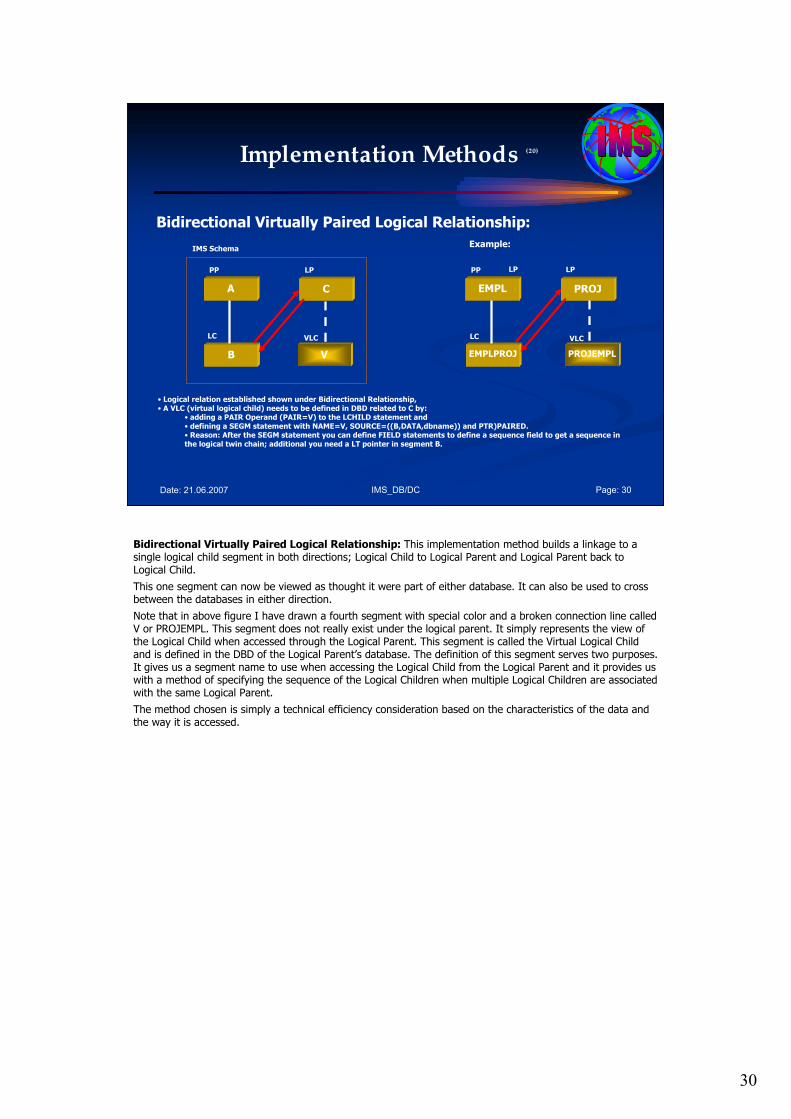
30
IMS_DB/DC Page: 30Date: 21.06.2007
Implementation Methods (20)
Bidirectional Virtually Paired Logical Relationship:
• Logical relation established shown under Bidirectional Relationship,• A VLC (virtual logical child) needs to be defined in DBD related to C by:
• adding a PAIR Operand (PAIR=V) to the LCHILD statement and• defining a SEGM statement with NAME=V, SOURCE=((B,DATA,dbname)) and PTR)PAIRED.• Reason: After the SEGM statement you can define FIELD statements to define a sequence field to get a sequence in the logical twin chain; additional you need a LT pointer in segment B.
A
B
C
LPPP
LC
IMS Schema
V
VLC
EMPL
EMPLPROJ
PROJ
LPPP
LC
Example:
PROJEMPL
VLC
LP
Bidirectional Virtually Paired Logical Relationship: This implementation method builds a linkage to a single logical child segment in both directions; Logical Child to Logical Parent and Logical Parent back to Logical Child.
This one segment can now be viewed as thought it were part of either database. It can also be used to cross between the databases in either direction.
Note that in above figure I have drawn a fourth segment with special color and a broken connection line called V or PROJEMPL. This segment does not really exist under the logical parent. It simply represents the view of the Logical Child when accessed through the Logical Parent. This segment is called the Virtual Logical Child and is defined in the DBD of the Logical Parent’s database. The definition of this segment serves two purposes. It gives us a segment name to use when accessing the Logical Child from the Logical Parent and it provides us with a method of specifying the sequence of the Logical Children when multiple Logical Children are associated with the same Logical Parent.
The method chosen is simply a technical efficiency consideration based on the characteristics of the data and the way it is accessed.
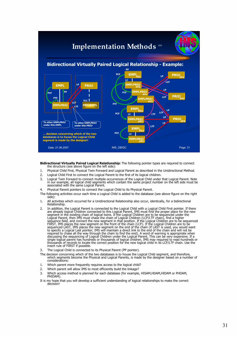
31
IMS_DB/DC Page: 31Date: 21.06.2007
Implementation Methods (21)
Bidirectional Virtually Paired Logical Relationship - Example:
EMPL
EMPLPROJ
PROJLP
PP
LC
PCF
EMPLPROJ
EMPLPROJ
#P2
#P1
#P3
#P1
PROJ#P2
PROJ#P3
#E1
LP
LPEMPL
EMPLPROJ
LC
#P3
#E2
EMPL
EMPLPROJ
LC
#P3
#E3
LP
LP
PTF
PTF
PCF
PCF
LCF
LCF
LCFLTF
LTF
To other EMPLPROJ under this EMPL
EMPL
EMPLPROJ
PROJLP
PP
LCFPROJEMPL
VLC
PCF
PTF
LTF
To other EMPLPROJ under this PROJ
… decision concerning which of the two databases is to house the Logical Child segment is made by the designer!
Bidirectional Virtually Paired Logical Relationship: The following pointer types are required to connect the structure (see above figure on the left side):
1. Physical Child First, Physical Twin Forward and Logical Parent as described in the Unidirectional Method.
2. Logical Child First to connect the Logical Parent to the first of its logical children.
3. Logical Twin Forward to connect multiple occurrences of the Logical Child under that Logical Parent. Note in our example, all logical child segments which contain the same project number on the left side must be associated with the same Logical Parent.
4. Physical Parent pointers to connect the Logical Child to its Physical Parent.
The following activities occur each time a Logical Child is added to the database (see above figure on the right side):
1. All activities which occurred for a Unidirectional Relationship also occur, identically, for a bidirectional Relationship.
2. In addition, the Logical Parent is connected to the Logical Child with a Logical Child First pointer. If there are already logical Children connected to this Logical Parent, IMS must find the proper place for the new segment in the existing chain of logical twins. If the Logical Children are to be sequenced under the Logical Parent, then IMS must chase the chain of Logical Children (LCF/LTF chain), find a higher sequence field, and connect the new segment in that position. If the Logical Children are to be sequenced FIRST, IMS places the new segment on the front of the chain (LCF). If the Logical Children are to be sequenced LAST, IMS places the new segment on the end of the chain (if LAST is used, you would want to specify a Logical Last pointer; IMS will maintain a direct link to the end of the chain and will not be required to chase all the way through the chain to find the end). A word of warning is appropriate when discussing the sequencing of Logical Children under the Logical Parent. This can be very expensive. If a single logical parent has hundreds or thousands of logical children, IMS may required to read hundreds or thousands of records to locate the correct position for the new logical child in its LCF/LTF chain. Use the insert rule of FIRST if possible.
3. The Logical Child is connected to its Physical Parent (PP pointer).
The decision concerning which of the two databases is to house the Logical Child segment, and therefore, which segments become the Physical and Logical Parents, is made by the designer based on a number of considerations:
1. Which parent more frequently requires access to the logical child?
2. Which parent will allow IMS to most efficiently build the linkage?
3. Which access method is planned for each database (for example, HISAM,HDAM,HIDAM or PHDAM, PHIDAM).
It is my hope that you will develop a sufficient understanding of logical relationships to make the correct decision!
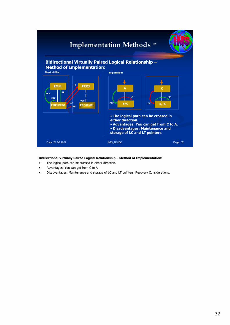
32
IMS_DB/DC Page: 32Date: 21.06.2007
Implementation Methods (22)
Bidirectional Virtually Paired Logical Relationship –Method of Implementation:
EMPL
EMPLPROJ
PROJLP
PP
LCFPROJEMPL
VLC
PCF
PTF
LTF
Physical DB’s: Logical DB’s:
A
B/CPCF
LP
C
BV/ALCF
PP
• The logical path can be crossed in either direction.• Advantages: You can get from C to A.• Disadvantages: Maintenance and storage of LC and LT pointers.
Bidirectional Virtually Paired Logical Relationship – Method of Implementation:
• The logical path can be crossed in either direction.
• Advantages: You can get from C to A.
• Disadvantages: Maintenance and storage of LC and LT pointers. Recovery Considerations.

33
IMS_DB/DC Page: 33Date: 21.06.2007
Implementation Methods (23)
Defining Sequence Fields for Logical Relationships:
This topic discusses defining the following types of sequence fields:
• “Logical Parent Sequence Fields”
• “Real Logical Children Sequence Fields”
• “Virtual Logical Children Sequence Fields”
Defining Sequence Fields for Logical Relationships: This topic discusses defining the following types of sequence fields:
• Logical Parent Sequence Fields: To avoid potential problems in processing databases using logical relationships, unique sequence fields should be defined in all logical parent segments. In all segments a logical parent is dependent on in its physical database. When unique sequence fields are not defined in all segments on the path to and including a logical parent, multiple logical parents in a database can have the same concatenated key. When this happens, problems can arise during and after initial database load when symbolic logical parent pointers in logical child segments are used to establish position on a logical parent segment. At initial database load time, if logical parents with non-unique concatenated keys exist in a database, the resolution utilities attach all logical children with the same concatenated key to the first logical parent in the database with that concatenated key. When inserting or deleting a concatenated segment and position for the logical parent, part of the concatenated segment is determined by the logical parent’s concatenated key. Positioning for the logical parent starts at the root and stops on the first segment at each level of the logical parent’s database that satisfies the key equal condition for that level. If a segment is missing on the path to the logical parent being inserted, a GE status code is returned to the application program when using this method to establish position in the logical parent’s database.
• Real Logical Children Sequence Fields: If the sequence field of a real logical child consists of any part of the logical parent’s concatenated key, PHYSICAL must be specified on the PARENT= parameter in the SEGM statement for the logical child. This will cause the concatenated key of the logical parent to be stored with the logical child segment.
• Virtual Logical Children Sequence Fields: As a general rule, a segment can have only one sequence field. However, in the case of virtual pairing, multiple FIELD statements can be used to define a logical sequence field for the virtual logical child. A sequence field must be specified for a virtual logical child if, when accessing it from its logical parent, you need real logical child segments retrieved in an order determined by data in a field of the virtual logical child as it could be seen in the application program I/O area. This sequence field can include any part of the segment as it appears when viewed from the logical parent (that is, the concatenated key of the real logical child’s physical parent followed by any intersection data). Because it can be necessary to describe the sequence field of a logical child as accessed from its logical parent in non-contiguous pieces, multiple FIELD statements with the SEQ parameter present are permitted. Each statement must contain a unique fldname1 parameter.

34
IMS_DB/DC Page: 34Date: 21.06.2007
Agenda Session 4: Logical Relationships /Logical Databases
1. Logical Relationships
2. Implementation Methods
• Unidirectional Relationship
• Bidirectional physically paired logical Relationships
• Bidirectional virtually paired logical Relationships
3. Paths in Logical Relationships
4. Logical Databases
5. Closing Comments
3. Paths in Logical Relationships.
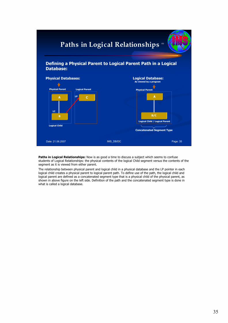
35
IMS_DB/DC Page: 35Date: 21.06.2007
Paths in Logical Relationships (1)
Defining a Physical Parent to Logical Parent Path in a LogicalDatabase:
Physical Databases:
A
B
CLP
LC
Physical Parent Logical Parent
Logical Child
A
B/C
Logical Database:
Logical Child / Logical Parent
Concatenated Segment Type
Physical Parent
As viewed by a program
Paths in Logical Relationships: Now is as good a time to discuss a subject which seems to confuse students of Logical Relationships: the physical contents of the logical Child segment versus the contents of the segment as it is viewed from either parent.
The relationship between physical parent and logical child in a physical database and the LP pointer in each logical child creates a physical parent to logical parent path. To define use of the path, the logical child and logical parent are defined as a concatenated segment type that is a physical child of the physical parent, as shown in above figure on the left side. Definition of the path and the concatenated segment type is done in what is called a logical database.
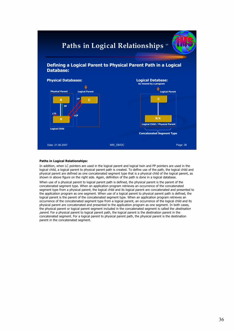
36
IMS_DB/DC Page: 36Date: 21.06.2007
Paths in Logical Relationships (2)
Defining a Logical Parent to Physical Parent Path in a LogicalDatabase:
Physical Databases: Logical Database:
A
B
CLP
LTF
Physical Parent Logical Parent
Logical Child
LCF
PP
C
B/A
Logical Child / Physical Parent
Concatenated Segment Type
Logical Parent
As viewed by a program
Paths in Logical Relationships:
In addition, when LC pointers are used in the logical parent and logical twin and PP pointers are used in the logical child, a logical parent to physical parent path is created. To define use of the path, the logical child and physical parent are defined as one concatenated segment type that is a physical child of the logical parent, as shown in above figure on the right side. Again, definition of the path is done in a logical database.
When use of a physical parent to logical parent path is defined, the physical parent is the parent of the concatenated segment type. When an application program retrieves an occurrence of the concatenated segment type from a physical parent, the logical child and its logical parent are concatenated and presented to the application program as one segment. When use of a logical parent to physical parent path is defined, the logical parent is the parent of the concatenated segment type. When an application program retrieves an occurrence of the concatenated segment type from a logical parent, an occurrence of the logical child and its physical parent are concatenated and presented to the application program as one segment. In both cases, the physical parent or logical parent segment included in the concatenated segment is called the destination parent. For a physical parent to logical parent path, the logical parent is the destination parent in the concatenated segment. For a logical parent to physical parent path, the physical parent is the destination parent in the concatenated segment.
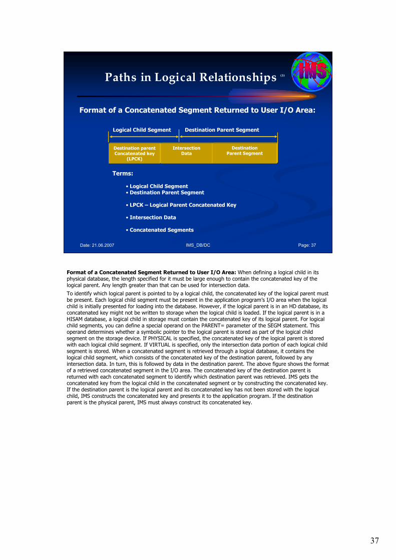
37
IMS_DB/DC Page: 37Date: 21.06.2007
Paths in Logical Relationships (3)
Format of a Concatenated Segment Returned to User I/O Area:
Destination parentConcatenated key
(LPCK)
IntersectionData
DestinationParent Segment
Logical Child Segment Destination Parent Segment
Terms:
• Logical Child Segment• Destination Parent Segment
• LPCK – Logical Parent Concatenated Key
• Intersection Data
• Concatenated Segments
Format of a Concatenated Segment Returned to User I/O Area: When defining a logical child in its physical database, the length specified for it must be large enough to contain the concatenated key of the logical parent. Any length greater than that can be used for intersection data.
To identify which logical parent is pointed to by a logical child, the concatenated key of the logical parent must be present. Each logical child segment must be present in the application program’s I/O area when the logical child is initially presented for loading into the database. However, if the logical parent is in an HD database, its concatenated key might not be written to storage when the logical child is loaded. If the logical parent is in a HISAM database, a logical child in storage must contain the concatenated key of its logical parent. For logical child segments, you can define a special operand on the PARENT= parameter of the SEGM statement. This operand determines whether a symbolic pointer to the logical parent is stored as part of the logical child segment on the storage device. If PHYSICAL is specified, the concatenated key of the logical parent is stored with each logical child segment. If VIRTUAL is specified, only the intersection data portion of each logical child segment is stored. When a concatenated segment is retrieved through a logical database, it contains the logical child segment, which consists of the concatenated key of the destination parent, followed by any intersection data. In turn, this is followed by data in the destination parent. The above figure shows the format of a retrieved concatenated segment in the I/O area. The concatenated key of the destination parent is returned with each concatenated segment to identify which destination parent was retrieved. IMS gets the concatenated key from the logical child in the concatenated segment or by constructing the concatenated key. If the destination parent is the logical parent and its concatenated key has not been stored with the logical child, IMS constructs the concatenated key and presents it to the application program. If the destination parent is the physical parent, IMS must always construct its concatenated key.
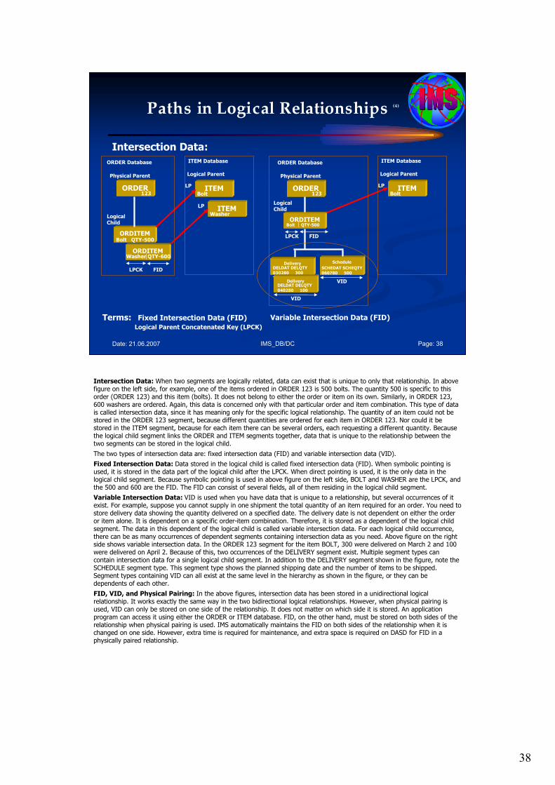
38
IMS_DB/DC Page: 38Date: 21.06.2007
Paths in Logical Relationships (4)
Intersection Data:
ORDER
ORDITEM
ITEMLP
Physical Parent Logical Parent
LogicalChild
ORDITEM
Bolt QTY-500
Washer QTY-600
Bolt
ITEMLP
Washer
123
LPCK FID
ORDER Database ITEM Database
Terms: Fixed Intersection Data (FID)
Logical Parent Concatenated Key (LPCK)
Variable Intersection Data (FID)
ORDER
ORDITEM
ITEMLP
Physical Parent Logical Parent
LogicalChild
Delivery
Bolt QTY-500
Bolt 123
VID
ORDER Database ITEM Database
Schedule
VIDDelivery
VID
SCHEDAT SCHEQTY060780 500
DELDAT DELQTY030280 300
DELDAT DELQTY040280 100
LPCK FID
Intersection Data: When two segments are logically related, data can exist that is unique to only that relationship. In above figure on the left side, for example, one of the items ordered in ORDER 123 is 500 bolts. The quantity 500 is specific to this order (ORDER 123) and this item (bolts). It does not belong to either the order or item on its own. Similarly, in ORDER 123, 600 washers are ordered. Again, this data is concerned only with that particular order and item combination. This type of data is called intersection data, since it has meaning only for the specific logical relationship. The quantity of an item could not be stored in the ORDER 123 segment, because different quantities are ordered for each item in ORDER 123. Nor could it be stored in the ITEM segment, because for each item there can be several orders, each requesting a different quantity. Because the logical child segment links the ORDER and ITEM segments together, data that is unique to the relationship between the two segments can be stored in the logical child.
The two types of intersection data are: fixed intersection data (FID) and variable intersection data (VID).
Fixed Intersection Data: Data stored in the logical child is called fixed intersection data (FID). When symbolic pointing is used, it is stored in the data part of the logical child after the LPCK. When direct pointing is used, it is the only data in the logical child segment. Because symbolic pointing is used in above figure on the left side, BOLT and WASHER are the LPCK, and the 500 and 600 are the FID. The FID can consist of several fields, all of them residing in the logical child segment.
Variable Intersection Data: VID is used when you have data that is unique to a relationship, but several occurrences of it exist. For example, suppose you cannot supply in one shipment the total quantity of an item required for an order. You need to store delivery data showing the quantity delivered on a specified date. The delivery date is not dependent on either the order or item alone. It is dependent on a specific order-item combination. Therefore, it is stored as a dependent of the logical child segment. The data in this dependent of the logical child is called variable intersection data. For each logical child occurrence, there can be as many occurrences of dependent segments containing intersection data as you need. Above figure on the right side shows variable intersection data. In the ORDER 123 segment for the item BOLT, 300 were delivered on March 2 and 100 were delivered on April 2. Because of this, two occurrences of the DELIVERY segment exist. Multiple segment types can contain intersection data for a single logical child segment. In addition to the DELIVERY segment shown in the figure, note the SCHEDULE segment type. This segment type shows the planned shipping date and the number of items to be shipped. Segment types containing VID can all exist at the same level in the hierarchy as shown in the figure, or they can be dependents of each other.
FID, VID, and Physical Pairing: In the above figures, intersection data has been stored in a unidirectional logical relationship. It works exactly the same way in the two bidirectional logical relationships. However, when physical pairing is used, VID can only be stored on one side of the relationship. It does not matter on which side it is stored. An application program can access it using either the ORDER or ITEM database. FID, on the other hand, must be stored on both sides of the relationship when physical pairing is used. IMS automatically maintains the FID on both sides of the relationship when it is changed on one side. However, extra time is required for maintenance, and extra space is required on DASD for FID in a physically paired relationship.

39
IMS_DB/DC Page: 39Date: 21.06.2007
Paths in Logical Relationships (5)
Contents of the Logical Child Segment – as viewed by a program:
EMPL
PP
Empl# Name etc.
EMPLOYEE Database PROJECT Database
EMPLPROJProj# Start Total
Date Hrs.
LC
PROJ
Proj# Descr. etc.
LPCK
Note: LPCK may not physically be stored on the DB,but is every time shown on the left side of the Program I/O area!
Contents of the Logical Child Segment – as viewed by a program: For all three implementation methods, the designer has a choice of whether or not to physically store the Logical Parent’s concatenated key (LPCK) in the logical child segment. This choice does not affect the application program’s view of the logical child segment! IMS will always return the LPCK in the program’s I/O area for the logical child, even though the LPCK may not physically be stored on the database.With the Unidirectional method, there is no problem since the Logical Child may only be accessed through the physical parent. The logical child I/O area will contain the key of the logical parent, left justified in the segment, followed by any amount of other data elements (Intersection Data). The segment will be viewed by a program as illustrated in the above figure.
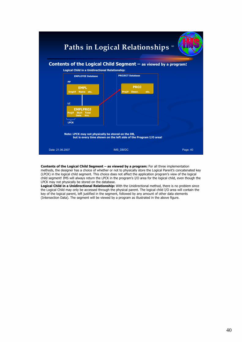
40
IMS_DB/DC Page: 40Date: 21.06.2007
Paths in Logical Relationships (6)
Contents of the Logical Child Segment – as viewed by a program:
Note: LPCK may not physically be stored on the DB,but is every time shown on the left side of the Program I/O area!
EMPL
PP
Empl# Name etc.
EMPLOYEE Database PROJECT Database
EMPLPROJProj# Start Total
Date Hrs.
LC
PROJ
Proj# Descr. etc.
LPCK
Logical Child in a Unidirectional Relationship:
Contents of the Logical Child Segment – as viewed by a program: For all three implementation methods, the designer has a choice of whether or not to physically store the Logical Parent’s concatenated key (LPCK) in the logical child segment. This choice does not affect the application program’s view of the logical child segment! IMS will always return the LPCK in the program’s I/O area for the logical child, even though the LPCK may not physically be stored on the database.Logical Child in a Unidirectional Relationship: With the Unidirectional method, there is no problem since the Logical Child may only be accessed through the physical parent. The logical child I/O area will contain the key of the logical parent, left justified in the segment, followed by any amount of other data elements (Intersection Data). The segment will be viewed by a program as illustrated in the above figure.
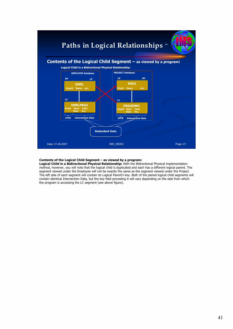
41
IMS_DB/DC Page: 41Date: 21.06.2007
Paths in Logical Relationships (6)
Contents of the Logical Child Segment – as viewed by a program:
EMPL
PP
Empl# Name etc.
EMPLOYEE Database PROJECT Database
EMPLPROJProj# Start Total
Date Hrs.
LC
PROJ
Proj# Descr. etc.
LPCK
Redundant Data
Logical Child in a Bidirectional Physical Relationship:
PROJEMPLEmpl# Start Total
Date Hrs.
LC
LPCK
PPLP LP
Intersection Data Intersection Data
Contents of the Logical Child Segment – as viewed by a program: Logical Child in a Bidirectional Physical Relationship: With the Bidirectional Physical implementation method, however, you will note that the logical child is duplicated and each has a different logical parent. The segment viewed under the Employee will not be exactly the same as the segment viewed under the Project. The left side of each segment will contain its Logical Parent’s key. Both of the paired logical child segments will contain identical Intersection Data, but the key field preceding it will vary depending on the side from which the program is accessing the LC segment (see above figure).
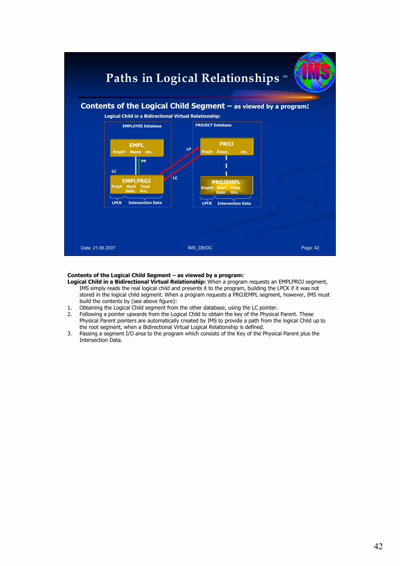
42
IMS_DB/DC Page: 42Date: 21.06.2007
Paths in Logical Relationships (6)
Contents of the Logical Child Segment – as viewed by a program:
EMPL
PP
Empl# Name etc.
EMPLOYEE Database PROJECT Database
EMPLPROJProj# Start Total
Date Hrs.
LC
PROJ
Proj# Descr. etc.
LPCK
Logical Child in a Bidirectional Virtual Relationship:
PROJEMPLEmpl# Start Total
Date Hrs.
LC
LPCK
LP
Intersection Data Intersection Data
Contents of the Logical Child Segment – as viewed by a program: Logical Child in a Bidirectional Virtual Relationship: When a program requests an EMPLPROJ segment,
IMS simply reads the real logical child and presents it to the program, building the LPCK if it was not stored in the logical child segment. When a program requests a PROJEMPL segment, however, IMS must build the contents by (see above figure):
1. Obtaining the Logical Child segment from the other database, using the LC pointer.2. Following a pointer upwards from the Logical Child to obtain the key of the Physical Parent. These
Physical Parent pointers are automatically created by IMS to provide a path from the logical Child up to the root segment, when a Bidirectional Virtual Logical Relationship is defined.
3. Passing a segment I/O area to the program which consists of the Key of the Physical Parent plus the Intersection Data.
43
IMS_DB/DC Page: 43Date: 21.06.2007
Paths in Logical Relationships (7)
Modifying the Logical Child Segment :
… 3 Fields are used to connect the structure:
• the key of the Logical Parent,• the sequence field for the Logical Child under its Physical Parent,• the sequence field for the Logical Child under its Logical Parent.
• IMS will not allow a program to update any of these fields!• program needs to delete the logical Child and rebuilt it to alter this data.
• physical BR: IMS must locate and correct paired segment any time it is updated from either side of the relationship.
Modifying the Logical Child Segment : The Logical Child segment has, potentially, three fields are used to connect the structure:
• the key of the Logical Parent,
• the sequence field for the Logical Child under its Physical Parent,
• the sequence field for the Logical Child under its Logical Parent.
IMS will not allow a program to update any of these fields because such an update would require a realignment of pointers. A program would, therefore, be required to delete the Logical Child and rebuilt it were necessary to alter this data.
There is one other consideration involved in the modification of data in the Logical Child segment when Bidirectional Physical method of implementation is chosen. Since the Logical Child segment exists in two places, IMS must locate and correct the paired segment any time it is updated from either side of the relationship. For this reason, it is seldom advisable to use Bidirectional Physical when the Intersection Data fields are highly volatile.
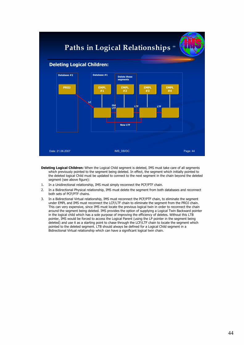
44
IMS_DB/DC Page: 44Date: 21.06.2007
Paths in Logical Relationships (8)
Deleting Logical Children:
PROJ EMPL#1
EMPL#2
EMPL#3
EMPL#4
LC
Old LTF
LTF LTF
Delete thesesegments
New LTF
Database #2 Database #1
Deleting Logical Children: When the Logical Child segment is deleted, IMS must take care of all segments which previously pointed to the segment being deleted. In effect, the segment which initially pointed to the deleted logical Child must be updated to connect to the next segment in the chain beyond the deleted segment (see above figure):
1. In a Unidirectional relationship, IMS must simply reconnect the PCF/PTF chain.
2. In a Bidirectional Physical relationship, IMS must delete the segment from both databases and reconnect both sets of PCF/PTF chains.
3. In a Bidirectional Virtual relationship, IMS must reconnect the PCF/PTF chain, to eliminate the segment under EMPL and IMS must reconnect the LCF/LTF chain to eliminate the segment from the PROJ chain. This can very expensive, since IMS must locate the previous logical twin in order to reconnect the chain around the segment being deleted. IMS provides the option of supplying a Logical Twin Backward pointer in the logical child which has a sole purpose of improving the efficiency of deletes. Without this LTB pointer, IMS would be forced to access the Logical Parent (using the LP pointer in the segment being deleted) and use it as a starting point to chase through the LCF/LTF chain to locate the segment which pointed to the deleted segment. LTB should always be defined for a Logical Child segment in a Bidirectional Virtual relationship which can have a significant logical twin chain.
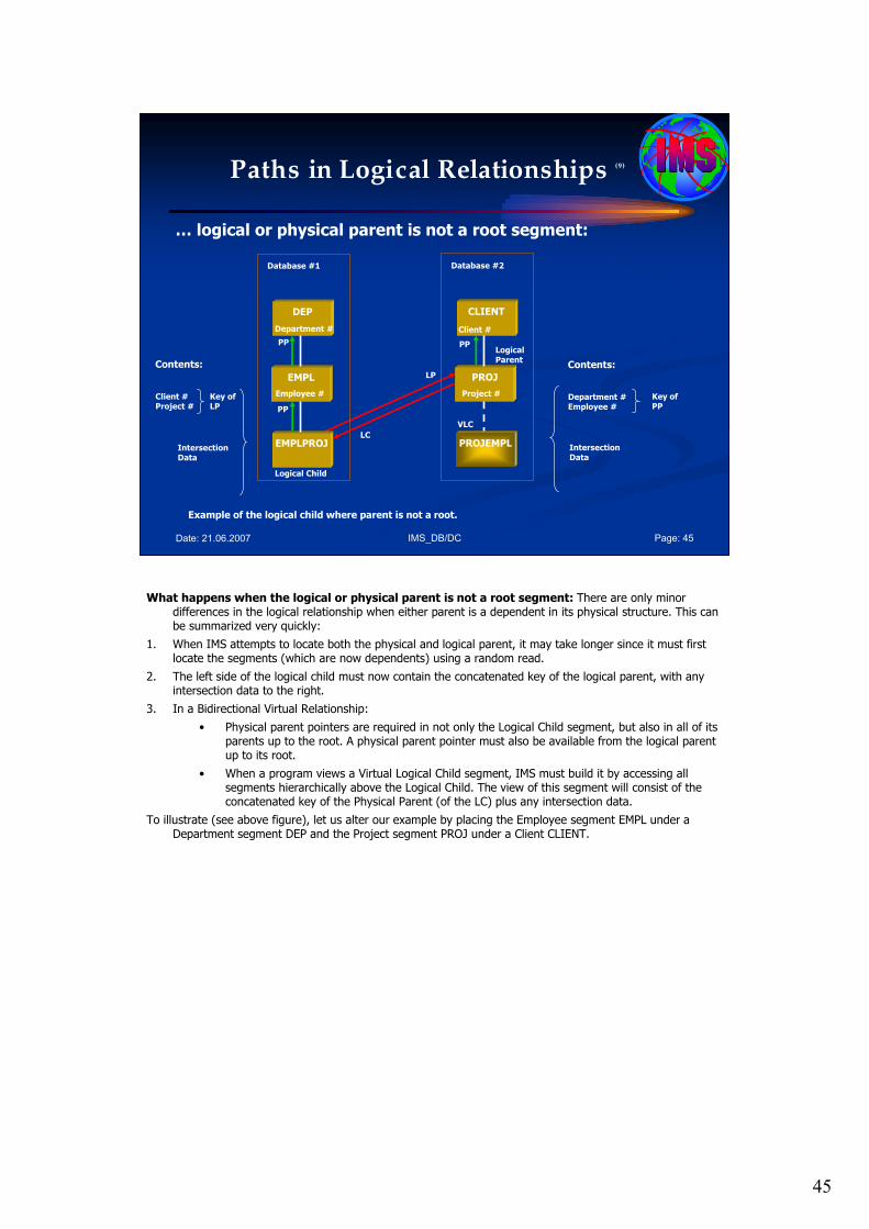
45
IMS_DB/DC Page: 45Date: 21.06.2007
Paths in Logical Relationships (9)
… logical or physical parent is not a root segment:
DEP
Database #1
EMPL
EMPLPROJLC
CLIENT
Database #2
PROJ
PROJEMPL
LP
PPPP
PP
Client #Project #
Key ofLP
IntersectionData
Logical Child
Logical Parent
VLC
Contents:
Department #Employee #
IntersectionData
Contents:
Key ofPP
Example of the logical child where parent is not a root.
Client #
Project #
Department #
Employee #
What happens when the logical or physical parent is not a root segment: There are only minor differences in the logical relationship when either parent is a dependent in its physical structure. This can be summarized very quickly:
1. When IMS attempts to locate both the physical and logical parent, it may take longer since it must first locate the segments (which are now dependents) using a random read.
2. The left side of the logical child must now contain the concatenated key of the logical parent, with any intersection data to the right.
3. In a Bidirectional Virtual Relationship:
• Physical parent pointers are required in not only the Logical Child segment, but also in all of its parents up to the root. A physical parent pointer must also be available from the logical parent up to its root.
• When a program views a Virtual Logical Child segment, IMS must build it by accessing all segments hierarchically above the Logical Child. The view of this segment will consist of the concatenated key of the Physical Parent (of the LC) plus any intersection data.
To illustrate (see above figure), let us alter our example by placing the Employee segment EMPL under a Department segment DEP and the Project segment PROJ under a Client CLIENT.
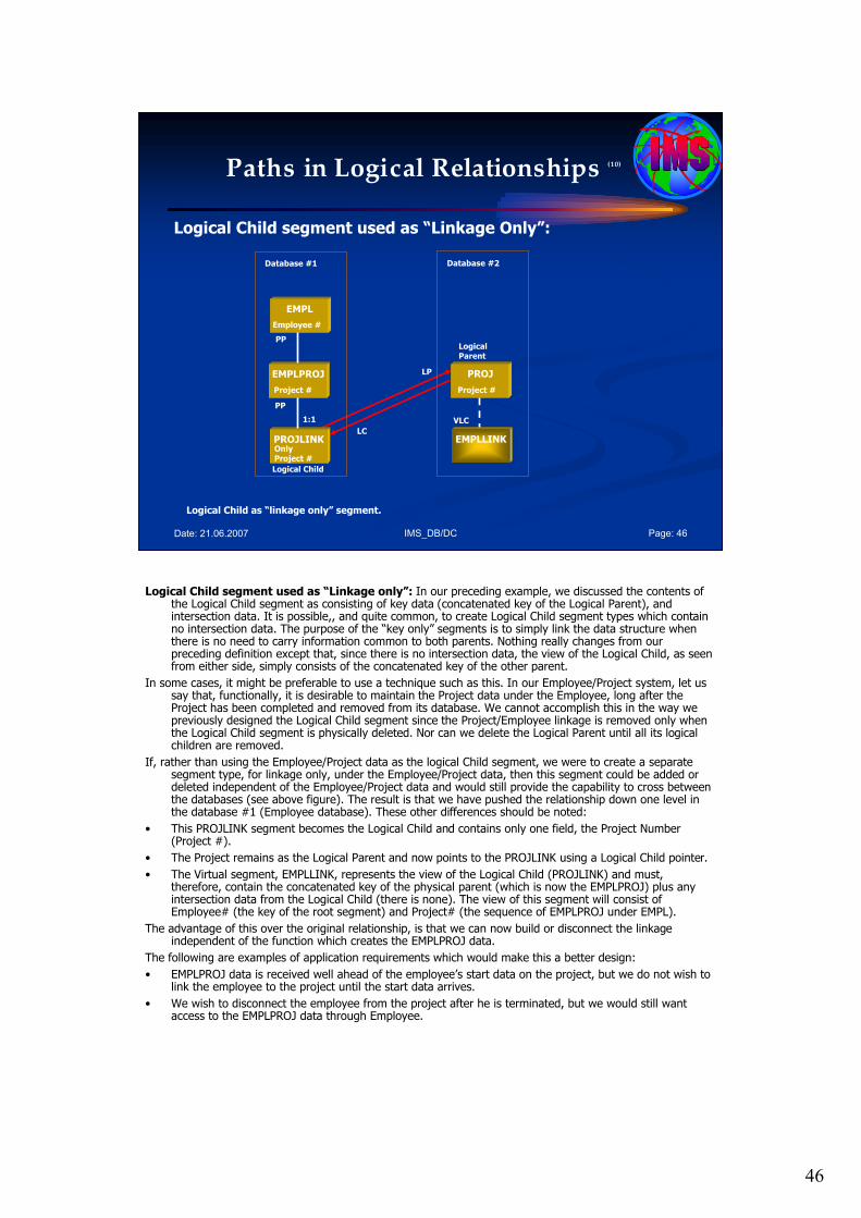
46
IMS_DB/DC Page: 46Date: 21.06.2007
Paths in Logical Relationships (10)
Logical Child segment used as “Linkage Only”:
EMPL
Database #1
EMPLPROJ
PROJLINKLC
Database #2
PROJ
EMPLLINK
LP
PP
PP
Logical Child
Logical Parent
VLC
Logical Child as “linkage only” segment.
Project #
1:1
Project #
Employee #
OnlyProject #
Logical Child segment used as “Linkage only”: In our preceding example, we discussed the contents of the Logical Child segment as consisting of key data (concatenated key of the Logical Parent), and intersection data. It is possible,, and quite common, to create Logical Child segment types which contain no intersection data. The purpose of the “key only” segments is to simply link the data structure when there is no need to carry information common to both parents. Nothing really changes from our preceding definition except that, since there is no intersection data, the view of the Logical Child, as seen from either side, simply consists of the concatenated key of the other parent.
In some cases, it might be preferable to use a technique such as this. In our Employee/Project system, let us say that, functionally, it is desirable to maintain the Project data under the Employee, long after the Project has been completed and removed from its database. We cannot accomplish this in the way we previously designed the Logical Child segment since the Project/Employee linkage is removed only when the Logical Child segment is physically deleted. Nor can we delete the Logical Parent until all its logical children are removed.
If, rather than using the Employee/Project data as the logical Child segment, we were to create a separate segment type, for linkage only, under the Employee/Project data, then this segment could be added or deleted independent of the Employee/Project data and would still provide the capability to cross between the databases (see above figure). The result is that we have pushed the relationship down one level in the database #1 (Employee database). These other differences should be noted:
• This PROJLINK segment becomes the Logical Child and contains only one field, the Project Number (Project #).
• The Project remains as the Logical Parent and now points to the PROJLINK using a Logical Child pointer.
• The Virtual segment, EMPLLINK, represents the view of the Logical Child (PROJLINK) and must, therefore, contain the concatenated key of the physical parent (which is now the EMPLPROJ) plus any intersection data from the Logical Child (there is none). The view of this segment will consist of Employee# (the key of the root segment) and Project# (the sequence of EMPLPROJ under EMPL).
The advantage of this over the original relationship, is that we can now build or disconnect the linkage independent of the function which creates the EMPLPROJ data.
The following are examples of application requirements which would make this a better design:
• EMPLPROJ data is received well ahead of the employee’s start data on the project, but we do not wish to link the employee to the project until the start data arrives.
• We wish to disconnect the employee from the project after he is terminated, but we would still want access to the EMPLPROJ data through Employee.

47
IMS_DB/DC Page: 47Date: 21.06.2007
Paths in Logical Relationships (11)
Selecting the most efficient Implementation Method:
… most common criteria:
1. If the logical relationship is only to be used to cross in one direction, from Physical Parent to Logical Parent, the Unidirectional Method should be selected.
2. If Bidirectional crossing is required and the following characteristics exist, Bidirectional Physical should be used:
3. Otherwise, use Bidirectional Virtual and attempt to talk the user out of sequencing the Logical Twins.
• The Logical Child is frequently accessed from both parents;• The intersection data is stable;• The requirement exists to sequence the Logical Child from bothsides, and the length of both chains may be significant.
Selecting the most efficient Implementation Method: The following represents the most common criteria for selecting the implementation method:
1. If the logical relationship is only to be used to cross in one direction, from Physical Parent to Logical Parent, the Unidirectional Method (UR) should be selected.
2. If Bidirectional crossing is required and the following characteristics exist, Bidirectional Physical should be used:
• The Logical Child is frequently accessed from both parents;
• The intersection data is stable;
• The requirement exists to sequence the Logical Child from both sides, and the length of both chains may be significant.
3. Otherwise, use Bidirectional Virtual and attempt to talk the user out of sequencing the Logical Twins.
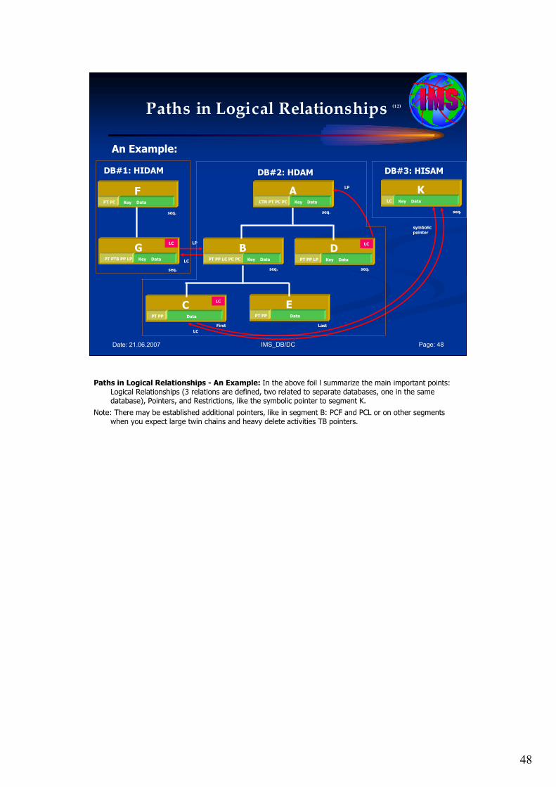
48
IMS_DB/DC Page: 48Date: 21.06.2007
Paths in Logical Relationships (12)
An Example:
FPT PC Key Data
GPT PTB PP LP Key Data
ACTR PT PC PC Key Data
BPT PP LC PC PC Key Data
KLC Key Data
DPT PP LP Key Data
CPT PP Data
EPT PP Data
LC LC
LC
LP
LC
LP
LC
symbolicpointer
DB#1: HIDAM DB#2: HDAM DB#3: HISAM
seq.
seq.
seq. seq.
seq. seq.
First Last
Paths in Logical Relationships - An Example: In the above foil l summarize the main important points: Logical Relationships (3 relations are defined, two related to separate databases, one in the same database), Pointers, and Restrictions, like the symbolic pointer to segment K.
Note: There may be established additional pointers, like in segment B: PCF and PCL or on other segments when you expect large twin chains and heavy delete activities TB pointers.

49
IMS_DB/DC Page: 49Date: 21.06.2007
Agenda Session 4: Logical Relationships /Logical Databases
1. Logical Relationships
2. Implementation Methods
• Unidirectional Relationship
• Bidirectional physically paired logical Relationships
• Bidirectional virtually paired logical Relationships
3. Paths in Logical Relationships
4. Logical Databases
5. Closing Comments
4. Logical Databases.
50
IMS_DB/DC Page: 50Date: 21.06.2007
Logical Databases (1)
Checklist of Rules for Defining Logical Databases:
Before the rules for defining logical databases can be described, you need to know the following definitions:
• Crossing a logical relationship
• The first and additional logical relationships crossed
Also, a logical DBD is needed only when an application program needs access to a concatenated segment or needs to cross a logical relationship.
Checklist of Rules for Defining Logical Databases: Before the rules for defining logical databases can be described, you need to know the following definitions:
• Crossing a logical relationship,
• The first and additional logical relationships crossed.
Also, a logical DBD is needed only when an application program needs access to a concatenated segment or needs to cross a logical relationship.
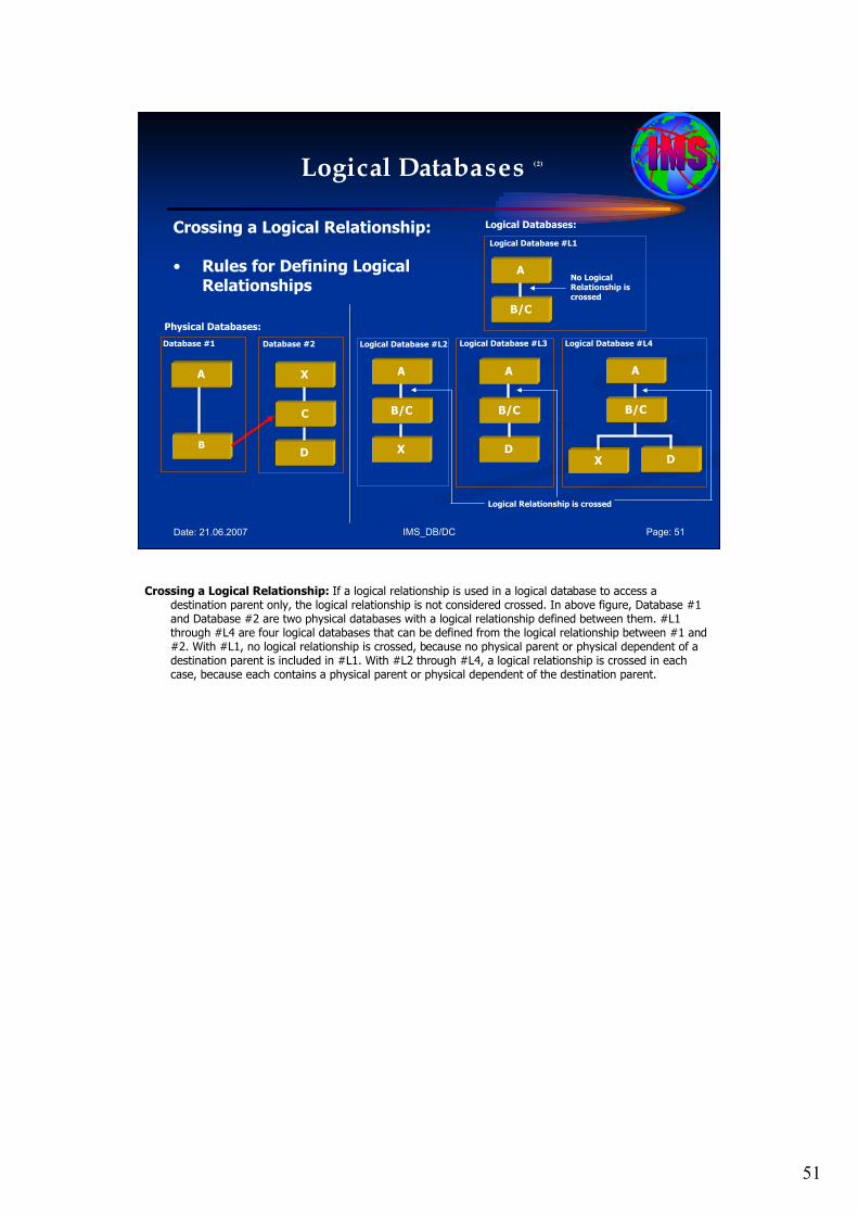
51
IMS_DB/DC Page: 51Date: 21.06.2007
Logical Databases (2)
Crossing a Logical Relationship:
• Rules for Defining Logical Relationships
A
B/C
Logical Database #L1
No Logical Relationship is crossed
Logical Databases:
A
B
X
Database #1 Database #2
C
D
Physical Databases:
A
B/C
X
A
B/C
D
A
B/C
X D
Logical Database #L2 Logical Database #L3 Logical Database #L4
Logical Relationship is crossed
Crossing a Logical Relationship: If a logical relationship is used in a logical database to access a destination parent only, the logical relationship is not considered crossed. In above figure, Database #1 and Database #2 are two physical databases with a logical relationship defined between them. #L1 through #L4 are four logical databases that can be defined from the logical relationship between #1 and #2. With #L1, no logical relationship is crossed, because no physical parent or physical dependent of a destination parent is included in #L1. With #L2 through #L4, a logical relationship is crossed in each case, because each contains a physical parent or physical dependent of the destination parent.
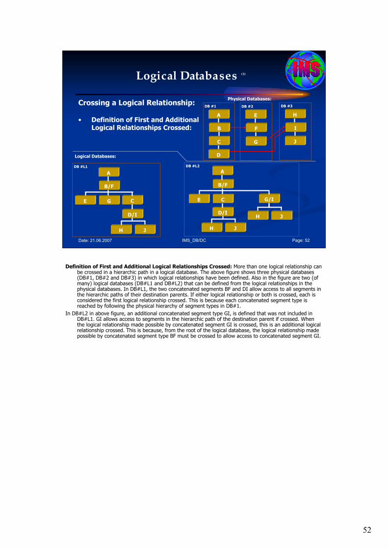
52
IMS_DB/DC Page: 52Date: 21.06.2007
Logical Databases (3)
Crossing a Logical Relationship:
• Definition of First and Additional Logical Relationships Crossed:
Physical Databases:
A
DB #1
B
C
D
E
DB #2
F
G
H
DB #3
I
J
Logical Databases:
A
B/F
GE C
D/I
JH
A
B/F
CE G/I
D/I
JH
JH
DB #L1 DB #L2
Definition of First and Additional Logical Relationships Crossed: More than one logical relationship can be crossed in a hierarchic path in a logical database. The above figure shows three physical databases (DB#1, DB#2 and DB#3) in which logical relationships have been defined. Also in the figure are two (of many) logical databases (DB#L1 and DB#L2) that can be defined from the logical relationships in the physical databases. In DB#L1, the two concatenated segments BF and DI allow access to all segments in the hierarchic paths of their destination parents. If either logical relationship or both is crossed, each is considered the first logical relationship crossed. This is because each concatenated segment type is reached by following the physical hierarchy of segment types in DB#1.
In DB#L2 in above figure, an additional concatenated segment type GI, is defined that was not included in DB#L1. GI allows access to segments in the hierarchic path of the destination parent if crossed. When the logical relationship made possible by concatenated segment GI is crossed, this is an additional logical relationship crossed. This is because, from the root of the logical database, the logical relationship made possible by concatenated segment type BF must be crossed to allow access to concatenated segment GI.
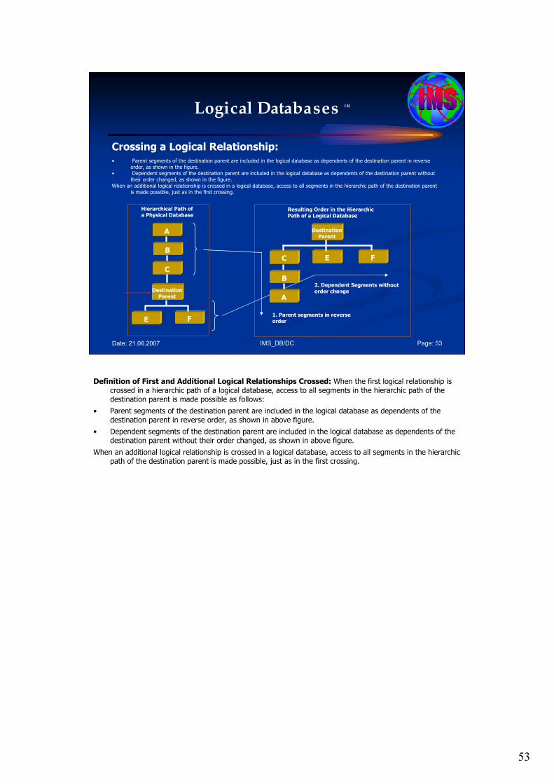
53
IMS_DB/DC Page: 53Date: 21.06.2007
Logical Databases (4)
Crossing a Logical Relationship:• Parent segments of the destination parent are included in the logical database as dependents of the destination parent in reverse
order, as shown in the figure. • Dependent segments of the destination parent are included in the logical database as dependents of the destination parent without
their order changed, as shown in the figure. When an additional logical relationship is crossed in a logical database, access to all segments in the hierarchic path of the destination parent
is made possible, just as in the first crossing.
A
Hierarchical Path of a Physical Database
B
C
DestinationParent
E F
DestinationParent
C E F
B
A
Resulting Order in the Hierarchic Path of a Logical Database
1. Parent segments in reverse order
2. Dependent Segments without order change
Definition of First and Additional Logical Relationships Crossed: When the first logical relationship is crossed in a hierarchic path of a logical database, access to all segments in the hierarchic path of the destination parent is made possible as follows:
• Parent segments of the destination parent are included in the logical database as dependents of the destination parent in reverse order, as shown in above figure.
• Dependent segments of the destination parent are included in the logical database as dependents of the destination parent without their order changed, as shown in above figure.
When an additional logical relationship is crossed in a logical database, access to all segments in the hierarchic path of the destination parent is made possible, just as in the first crossing.
54
IMS_DB/DC Page: 54Date: 21.06.2007
Logical Databases (5)
Rules for Defining Logical Databases:
• The root segment in a logical database must be the root segment in a physical database. • A logical database must use only those segments and physical and logical relationship paths defined in the physical DBD referenced by the logical DBD.• The path used to connect a parent and child in a logical database must be defined as a physical relationship path or a logical relationship path in the physical DBD referenced by the logical DBD. • Physical and logical relationship paths can be mixed in a hierarchic segment path in a logical database. • Additional physical relationship paths, logical relationship paths, or both paths can be included after a logical relationship is crossed in a hierarchic path in a logical database. These paths are included by going in upward directions, downward directions, or both directions, from the destination parent. When proceeding downward along a physical relationship path from the destination parent, direction cannot be changed except by crossing a logical relationship. When proceeding upward along a physical relationship path from the destination parent, direction can be changed. • Dependents in a logical database must be in the same relative order as they are under their parent in the physical database. If a segment in a logical database is a concatenated segment, the physical children of the logical child and children of the destination parent can be in any order. The relative order of the children or the logical child and the relative order of the children of the destination parent must remain unchanged. • The same concatenated segment type can be defined multiple times with different combinations of key and data sensitivity. Each must have a distinct name for that view of the concatenated segment. Only one of the views can have dependent segments.
Rules for Defining Logical Databases:
• The root segment in a logical database must be the root segment in a physical database.
• A logical database must use only those segments and physical and logical relationship paths defined in the physical DBD referenced by the logical DBD.
• The path used to connect a parent and child in a logical database must be defined as a physical relationship path or a logical relationship path in the physical DBD referenced by the logical DBD.
• Physical and logical relationship paths can be mixed in a hierarchic segment path in a logical database.
• Additional physical relationship paths, logical relationship paths, or both paths can be included after a logical relationship is crossed in a hierarchic path in a logical database. These paths are included by going in upward directions, downward directions, or both directions, from the destination parent. When proceeding downward along a physical relationship path from the destination parent, direction cannot be changed except by crossing a logical relationship. When proceeding upward along a physical relationship path from the destination parent, direction can be changed.
• Dependents in a logical database must be in the same relative order as they are under their parent in the physical database. If a segment in a logical database is a concatenated segment, the physical children of the logical child and children of the destination parent can be in any order. The relative order of the children or the logical child and the relative order of the children of the destination parent must remain unchanged.
• The same concatenated segment type can be defined multiple times with different combinations of key and data sensitivity. Each must have a distinct name for that view of the concatenated segment. Only one of the views can have dependent segments.
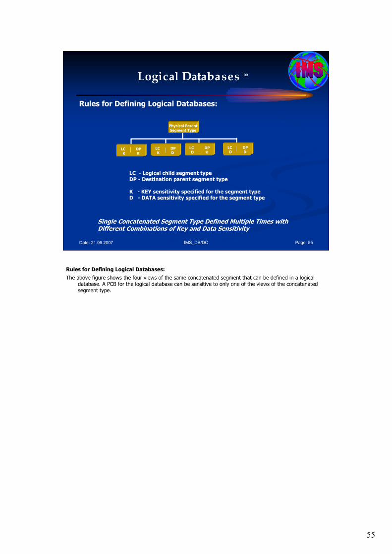
55
IMS_DB/DC Page: 55Date: 21.06.2007
Logical Databases (6)
Rules for Defining Logical Databases:
LC - Logical child segment type DP - Destination parent segment type
K - KEY sensitivity specified for the segment type D - DATA sensitivity specified for the segment type
Physical ParentSegment Type
LC DPK K
LC DPK D
LC DPD K
LC DPD D
Single Concatenated Segment Type Defined Multiple Times with Different Combinations of Key and Data Sensitivity
Rules for Defining Logical Databases:
The above figure shows the four views of the same concatenated segment that can be defined in a logical database. A PCB for the logical database can be sensitive to only one of the views of the concatenated segment type.
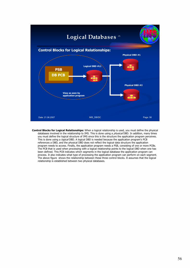
56
IMS_DB/DC Page: 56Date: 21.06.2007
Logical Databases (7)
Control Blocks for Logical Relationships:
PSB
DB PCB
Logical DBD #L1
Physical DBD #1
Physical DBD #2
View as seen by application program
Control Blocks for Logical Relationships: When a logical relationship is used, you must define the physical databases involved in the relationship to IMS. This is done using a physical DBD. In addition, many times you must define the logical structure of IMS since this is the structure the application program perceives. This is done using a logical DBD. A logical DBD is needed because the application program’s PCB references a DBD, and the physical DBD does not reflect the logical data structure the application program needs to access. Finally, the application program needs a PSB, consisting of one or more PCBs. The PCB that is used when processing with a logical relationship points to the logical DBD when one has been defined. This PCB indicates which segments in the logical database the application program can process. It also indicates what type of processing the application program can perform on each segment. The above figure shows the relationship between these three control blocks. It assumes that the logical relationship is established between two physical databases.
57
IMS_DB/DC Page: 57Date: 21.06.2007
Logical Databases (8)
Building Logical Data Structures:1. The Root segment in a logical structure must be a root segment in a physical structure.
2. The logical structure is defined to IMS through the use of a Logical DBD. The purpose of this logical DBD is as shown before simply to define the segment types to be included in the logical structure and to tell IMS which physical databases contain desired segments.
3. There are three paths which may followed in building a logical structure:
- Any or all of the physical dependents of a segment may be included in the logical structure. They must be defined in their normal
hierarchical structure.- If, in defining the segments to be included in our logical structure, we encounter a
Logical Child segment or Virtual Logical Childsegment, we may use that segment to cross into the related database. This is done
with the concatenated segment defined underCrossing a Logical Relationship.
- The logical crossover may be used to include, as dependents of the concatenated segment, the following:
- - Parents of the Destination Parent (the right hand side of the concatenation). These parents are inverted in the logical structure.
- - Children of the Logical Child.- - Children of the Destination Parent.
4. A single logical structure can cross into any number of different databases. Each time a Logical Child or Virtual logical Child is encountered, the option exists to build a concatenated segment and, thereby, gain access to the segments in the destination parent database.
Building Logical Data Structures: Once the linkage between databases has been established, we may build logical structures which allow us to view the contents of two or more physical databases in a single logical hierarchy.
The rules for building these logical structures are as shown before quite simple:
1. The Root segment in a logical structure must be a root segment in a physical structure.
2. The logical structure is defined to IMS through the use of a Logical DBD. The purpose of this logical DBD is as shown before simply to define the segment types to be included in the logical structure and to tell IMS which physical databases contain desired segments.
3. There are three paths which may followed in building a logical structure:
• Any or all of the physical dependents of a segment may be included in the logical structure. They must be defined in their normal hierarchical structure.
• If, in defining the segments to be included in our logical structure, we encounter a Logical Child segment or Virtual Logical Child segment, we may use that segment to cross into the related database. This is done with the concatenated segment defined under Crossing a Logical Relationship.
• The logical crossover may be used to include, as dependents of the concatenated segment, the following:
• Parents of the Destination Parent (the right hand side of the concatenation). These parents are inverted in the logical structure.
• Children of the Logical Child.
• Children of the Destination Parent.
4. A single logical structure can cross into any number of different databases. Each time a Logical Child or Virtual logical Child is encountered, the option exists to build a concatenated segment and, thereby, gain access to the segments in the destination parent database.
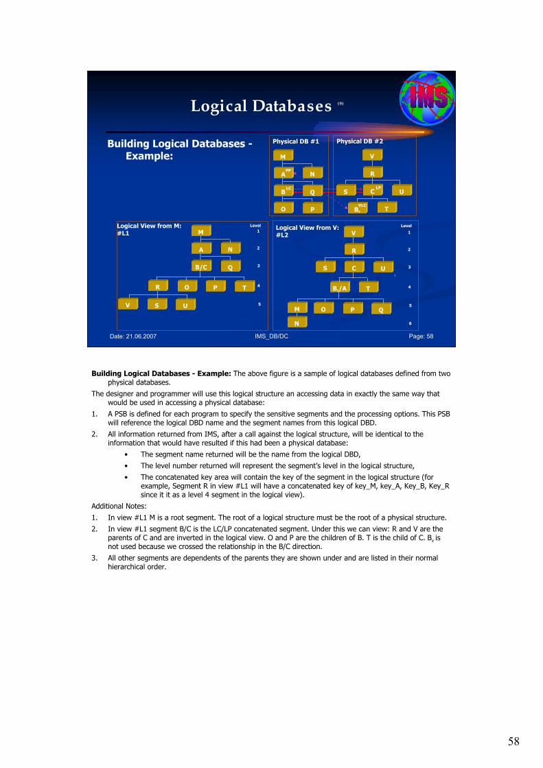
58
IMS_DB/DC Page: 58Date: 21.06.2007
Logical Databases (9)
Building Logical Databases -Example: M
A
B
O
N
Q
P
V
R
C
BV
S U
T
LPLC
PP
VLC
Physical DB #1 Physical DB #2
M
A
B/C
P
N
Q
TR O
UV S
Logical View from M:#L1 1
2
3
4
5
Level
V
R
C
T
S U
M
Bv/A
QO P
N
Logical View from V:#L2
1
2
3
4
5
6
Level
Building Logical Databases - Example: The above figure is a sample of logical databases defined from two physical databases.
The designer and programmer will use this logical structure an accessing data in exactly the same way that would be used in accessing a physical database:
1. A PSB is defined for each program to specify the sensitive segments and the processing options. This PSB will reference the logical DBD name and the segment names from this logical DBD.
2. All information returned from IMS, after a call against the logical structure, will be identical to the information that would have resulted if this had been a physical database:
• The segment name returned will be the name from the logical DBD,
• The level number returned will represent the segment’s level in the logical structure,
• The concatenated key area will contain the key of the segment in the logical structure (for example, Segment R in view #L1 will have a concatenated key of key_M, key_A, Key_B, Key_Rsince it it as a level 4 segment in the logical view).
Additional Notes:
1. In view #L1 M is a root segment. The root of a logical structure must be the root of a physical structure.
2. In view #L1 segment B/C is the LC/LP concatenated segment. Under this we can view: R and V are the parents of C and are inverted in the logical view. O and P are the children of B. T is the child of C. Bv is not used because we crossed the relationship in the B/C direction.
3. All other segments are dependents of the parents they are shown under and are listed in their normal hierarchical order.
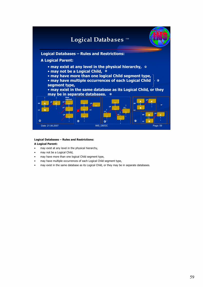
59
IMS_DB/DC Page: 59Date: 21.06.2007
Logical Databases (10)
Logical Databases – Rules and Restrictions:
A Logical Parent:
• may exist at any level in the physical hierarchy,• may not be a Logical Child,• may have more than one logical Child segment type,• may have multiple occurrences of each Logical Child segment type,• may exist in the same database as its Logical Child, or they may be in separate databases.
A
B
C
LC
PPLP
…
…
…
LP
LP
LP
1111
1111
…
…
…
LP
LC
…
2222
2222
…
…
……
…
LP
LC
LC
LC
3333
3333
Root segment
����
A
B
A’
LC
PP
LP
4444
A
B
C
LC
PPLP
or
4444
Logical Databases – Rules and Restrictions:
A Logical Parent:
• may exist at any level in the physical hierarchy,
• may not be a Logical Child,
• may have more than one logical Child segment type,
• may have multiple occurrences of each Logical Child segment type,
• may exist in the same database as its Logical Child, or they may be in separate databases.
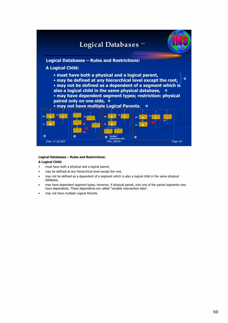
60
IMS_DB/DC Page: 60Date: 21.06.2007
Logical Databases (11)
Logical Databases – Rules and Restrictions:
A Logical Child:
• must have both a physical and a logical parent,• may be defined at any hierarchical level except the root,• may not be defined as a dependent of a segment which is also a logical child in the same physical database,• may have dependent segment types; restriction: physical paired only on one side,• may not have multiple Logical Parents.
A
B
C
LC
PPLP
1111
1111
…
…
…
LP
LC
…
2222
2222
3333
4444
����…
LC
A
B
C
LC
PPLP
3333
… …
Variable Intersection data
4444
A
B
C
LC
PPLP
…LP
����
Logical Databases – Rules and Restrictions:
A Logical Child:
• must have both a physical and a logical parent,
• may be defined at any hierarchical level except the root,
• may not be defined as a dependent of a segment which is also a logical child in the same physical database,
• may have dependent segment types; However, if physical paired, only one of the paired segments may have dependents. These dependents are called “variable intersection data”.
• may not have multiple Logical Parents.
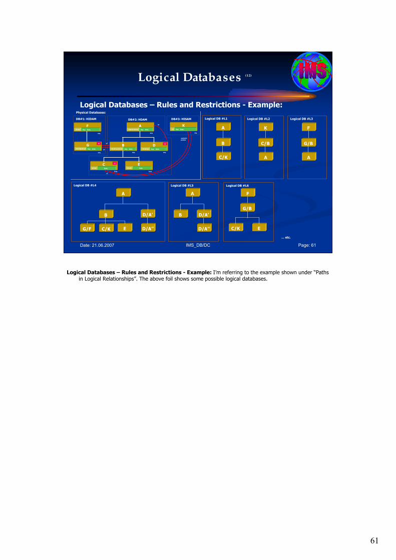
61
IMS_DB/DC Page: 61Date: 21.06.2007
Logical Databases (12)
Logical Databases – Rules and Restrictions - Example:Physical Databases:
FPT PC Key Data
GPT PTB PP LP Key Data
ACTR PT PC PC Key Data
BPT PP LC PC PC Key Data
KLC Key Data
DPT PP LP Key Data
CPT PP Data
EPT PP Data
LC LC
LC
LP
LC
LP
LC
symbolic
pointer
DB#1: HIDAM DB#2: HDAM DB#3: HISAM
seq.
seq.
seq. seq.
seq. seq.
First Last
A
B
C/K
Logical DB #L1
K
C/B
A
Logical DB #L2
F
G/B
A
Logical DB #L3
A
B
C/K
Logical DB #L4
G/F E
D/A’
D/A’’
A
B
Logical DB #L5
D/A’
D/A’’
F
C/K
Logical DB #L6
E
G/B
… etc.
Logical Databases – Rules and Restrictions - Example: I’m referring to the example shown under “Paths in Logical Relationships”. The above foil shows some possible logical databases.
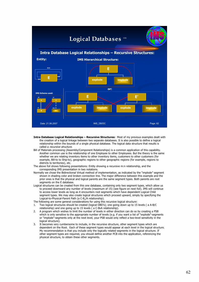
62
IMS_DB/DC Page: 62Date: 21.06.2007
Logical Databases (13)
Intra Database Logical Relationships – Recursive Structures:
E
implodeexplode
IMS Hierarchical Structure:
E
Entity:
m:n
E
implodeexplode
E’
implodeexplode
or:
A
B
C
LPPP
LC
V
VLC
IMS Schema used:
Intra Database Logical Relationships – Recursive Structures: Most of my previous examples dealt with the creation of a logical linkage between two separate databases. It is also possible to define a logical relationship within the bounds of a single physical database. The logical data structure that results is called a recursive structure.
Bill of Materials processing (Assembly/Component Relationships) is a common application of this capability. Another common use is the relationship of one Employee to other Employees. But the theory is the same whether we are relating inventory items to other inventory items, customers to other customers (for example, Bill-to to Ship-to), geographic regions to other geographic regions (for example, regions to districts to territories), etc.
The above foil shows following presentations: Entity showing a recursive m:n relationship, and the corresponding IMS presentation in two notations.
Normally we chose the Bidirectional Virtual method of implementation, as indicated by the “implode” segment shown in shading color and broken connection line. The major difference between this example and the prior ones is that the physical and logical parents are the same segment types. Both parents are root segments on the E database.
Logical structures can be created from this one database, containing only two segment types, which allow us to proceed downward any number of levels (maximum of 15) (see figure on next foil). IMS will continue to access lower levels as long as it encounters root segments which have dependent Logical Child segment types. We may also create logical structures which proceed upward, simply by specifying the Logical-to-Physical-Parent Path (a C-Bv/A relationship).
The following are some general considerations for using this recursive logical structure:1. Two logical structures should be created (logical DBD’s); one going down up to 15 levels ( a A-B/C
relationship) and one going up to 15 levels ( a C-BvA relationship). 2. A program which wishes to limit the number of levels in either direction can do so by creating a PSB
which is only sensitive to the appropriate number of levels (e.g. if you want a list of “explode”-segments or “implode”-segments only at the next level, your PSB would only reflect a two-level sensitivity in the logical structure).
3. It becomes very cumbersome to include, in the recursive structure, other segment types which are dependent on the Root. Each of these segment types would appear at each level in the logical structure. My recommendation is that you include only the logically related segments in the logical structure. If other segment types are required, you should define another PCB into the application, referencing the physical structure, to obtain these other segments.
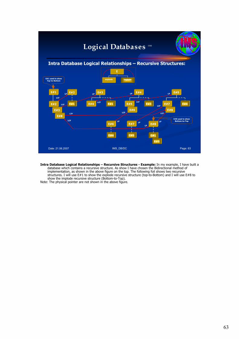
63
IMS_DB/DC Page: 63Date: 21.06.2007
Logical Databases (14)
Intra Database Logical Relationships – Recursive Structures:
E
implodeexplode
E#1
E#2 E#1 E#4 E#1 E#5 E#3 E#7 E#4
E#8E#6E#3
E#8
E#2 E#3 E#4 E#5
E#4
E#6
E#5
E#7
E#1
E#8
E#5
LCF
LCF
LP LP
LCF
LP
LCF
LP
LCF
LP
LCF
LPLP
LCFLTF
LP
LCF
E#1 used to showTop-to-Bottom
E#8 used to showBottom-to-Top
Intra Database Logical Relationships – Recursive Structures - Example: In my example, I have built a database which contains a recursive structure. As show I have chosen the Bidirectional method of implementation, as shown in the above figure on the top. The following foil shows two recursive structures. I will use E#1 to show the explode recursive structure (top-to-Bottom) and I will use E#8 to show the implode recursive structure (Bottom-to-Top).
Note: The physical pointer are not shown in the above figure.
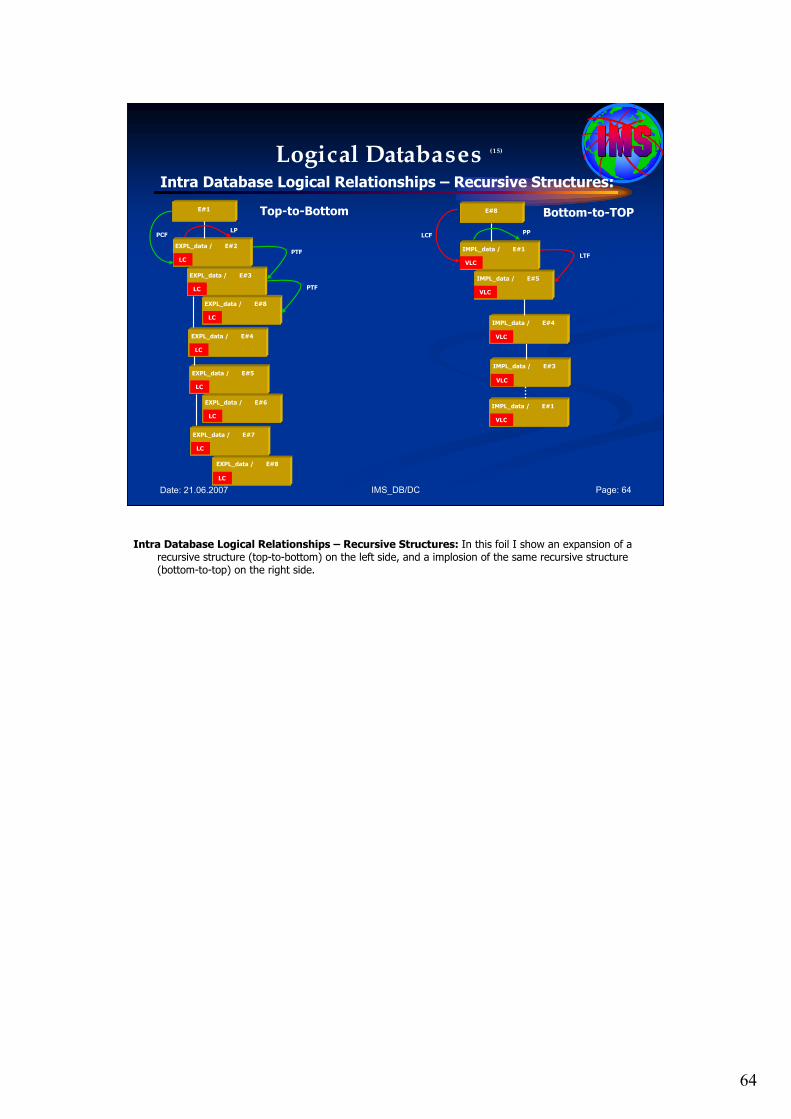
64
IMS_DB/DC Page: 64Date: 21.06.2007
Logical Databases (15)
Intra Database Logical Relationships – Recursive Structures:
E#8
VLC
IMPL_data / E#1
IMPL_data / E#5
IMPL_data / E#3
IMPL_data / E#1
IMPL_data / E#4
VLC
VLC
VLC
VLC
LCFPP
LTF
Bottom-to-TOP E#1
LC
EXPL_data / E#2
LC
EXPL_data / E#3
LC
EXPL_data / E#8
LC
EXPL_data / E#4
LC
EXPL_data / E#7
LC
EXPL_data / E#8
PCFLP
PTF
PTF
Top-to-Bottom
LC
EXPL_data / E#5
LC
EXPL_data / E#6
Intra Database Logical Relationships – Recursive Structures: In this foil I show an expansion of a recursive structure (top-to-bottom) on the left side, and a implosion of the same recursive structure (bottom-to-top) on the right side.
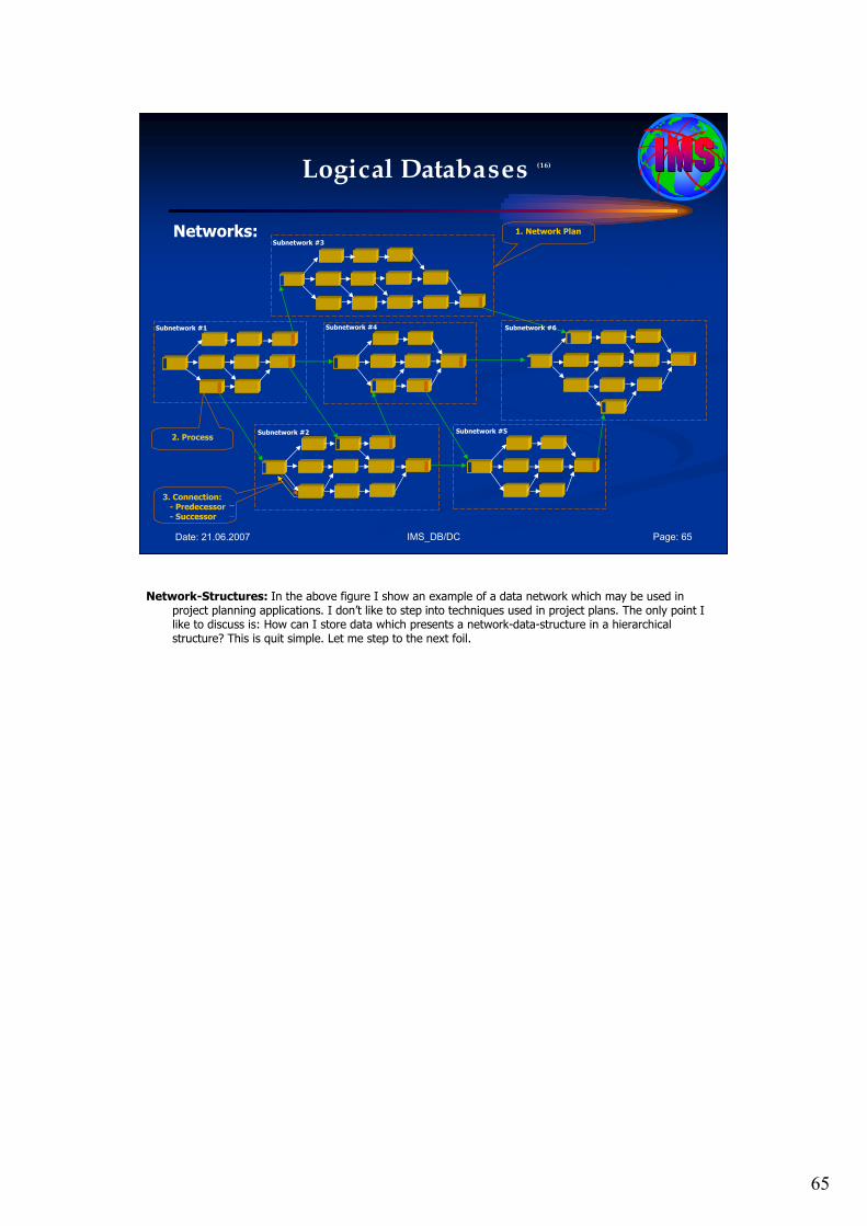
65
IMS_DB/DC Page: 65Date: 21.06.2007
Logical Databases (16)
Networks:Subnetwork #3
Subnetwork #1
Subnetwork #2
Subnetwork #4
Subnetwork #5
Subnetwork #6
1. Network Plan
2. Process
3. Connection:- Predecessor- Successor
Network-Structures: In the above figure I show an example of a data network which may be used in project planning applications. I don’t like to step into techniques used in project plans. The only point I like to discuss is: How can I store data which presents a network-data-structure in a hierarchical structure? This is quit simple. Let me step to the next foil.
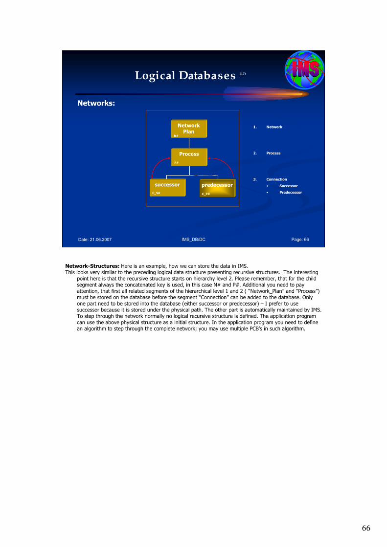
66
IMS_DB/DC Page: 66Date: 21.06.2007
Logical Databases (17)
Networks:
Process
predecessorsuccessor
NetworkPlan
N#
P#
C_S# C_P#
1. Network
2. Process
3. Connection
• Successor
• Predecessor
Network-Structures: Here is an example, how we can store the data in IMS. This looks very similar to the preceding logical data structure presenting recursive structures. The interesting
point here is that the recursive structure starts on hierarchy level 2. Please remember, that for the child segment always the concatenated key is used, in this case N# and P#. Additional you need to pay attention, that first all related segments of the hierarchical level 1 and 2 ( “Network_Plan” and “Process”) must be stored on the database before the segment “Connection” can be added to the database. Only one part need to be stored into the database (either successor or predecessor) – I prefer to use successor because it is stored under the physical path. The other part is automatically maintained by IMS. To step through the network normally no logical recursive structure is defined. The application program can use the above physical structure as a initial structure. In the application program you need to define an algorithm to step through the complete network; you may use multiple PCB’s in such algorithm.
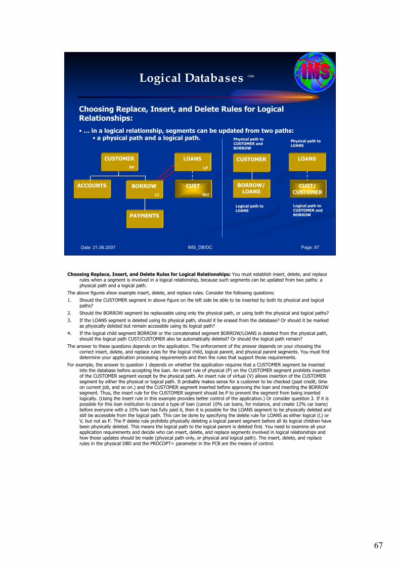
67
IMS_DB/DC Page: 67Date: 21.06.2007
Logical Databases (18)
Choosing Replace, Insert, and Delete Rules for Logical Relationships:
• … in a logical relationship, segments can be updated from two paths: • a physical path and a logical path.
CUSTOMER
ACCOUNTS BORROW
PAYMENTS
LOANS
CUST
PP
LC
LP
VLC
LOANS
CUST/CUSTOMER
CUSTOMER
BORROW/LOANS
Physical path toCUSTOMER andBORROW
Physical path toLOANS
Logical path toLOANS
Logical path toCUSTOMER and BORROW
Choosing Replace, Insert, and Delete Rules for Logical Relationships: You must establish insert, delete, and replace rules when a segment is involved in a logical relationship, because such segments can be updated from two paths: a physical path and a logical path.
The above figures show example insert, delete, and replace rules. Consider the following questions:
1. Should the CUSTOMER segment in above figure on the left side be able to be inserted by both its physical and logical paths?
2. Should the BORROW segment be replaceable using only the physical path, or using both the physical and logical paths?
3. If the LOANS segment is deleted using its physical path, should it be erased from the database? Or should it be marked as physically deleted but remain accessible using its logical path?
4. If the logical child segment BORROW or the concatenated segment BORROW/LOANS is deleted from the physical path, should the logical path CUST/CUSTOMER also be automatically deleted? Or should the logical path remain?
The answer to these questions depends on the application. The enforcement of the answer depends on your choosing the correct insert, delete, and replace rules for the logical child, logical parent, and physical parent segments. You must first determine your application processing requirements and then the rules that support those requirements.
For example, the answer to question 1 depends on whether the application requires that a CUSTOMER segment be inserted into the database before accepting the loan. An insert rule of physical (P) on the CUSTOMER segment prohibits insertion of the CUSTOMER segment except by the physical path. An insert rule of virtual (V) allows insertion of the CUSTOMER segment by either the physical or logical path. It probably makes sense for a customer to be checked (past credit, time on current job, and so on.) and the CUSTOMER segment inserted before approving the loan and inserting the BORROW segment. Thus, the insert rule for the CUSTOMER segment should be P to prevent the segment from being inserted logically. (Using the insert rule in this example provides better control of the application.) Or consider question 3. If it is possible for this loan institution to cancel a type of loan (cancel 10% car loans, for instance, and create 12% car loans) before everyone with a 10% loan has fully paid it, then it is possible for the LOANS segment to be physically deleted and still be accessible from the logical path. This can be done by specifying the delete rule for LOANS as either logical (L) or V, but not as P. The P delete rule prohibits physically deleting a logical parent segment before all its logical children have been physically deleted. This means the logical path to the logical parent is deleted first. You need to examine all your application requirements and decide who can insert, delete, and replace segments involved in logical relationships and how those updates should be made (physical path only, or physical and logical path). The insert, delete, and replace rules in the physical DBD and the PROCOPT= parameter in the PCB are the means of control.
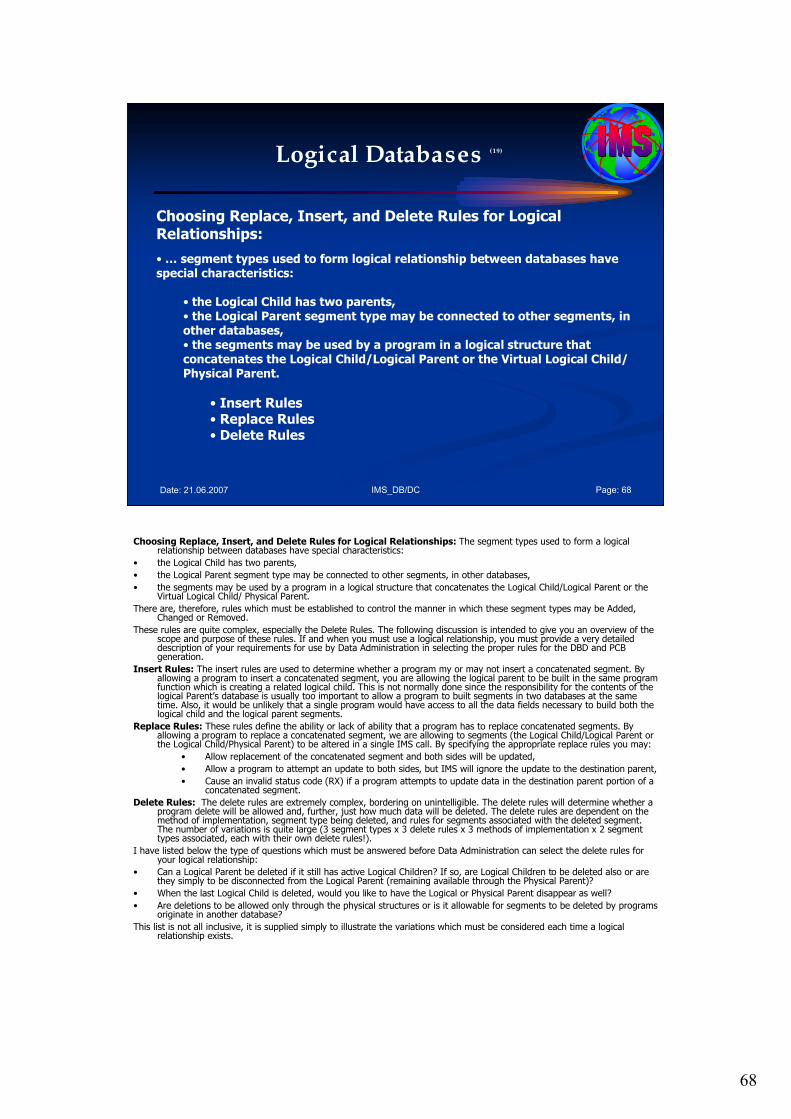
68
IMS_DB/DC Page: 68Date: 21.06.2007
Logical Databases (19)
Choosing Replace, Insert, and Delete Rules for Logical Relationships:
• … segment types used to form logical relationship between databases have special characteristics:
• the Logical Child has two parents,• the Logical Parent segment type may be connected to other segments, in other databases,• the segments may be used by a program in a logical structure that concatenates the Logical Child/Logical Parent or the Virtual Logical Child/ Physical Parent.
• Insert Rules• Replace Rules• Delete Rules
Choosing Replace, Insert, and Delete Rules for Logical Relationships: The segment types used to form a logical relationship between databases have special characteristics:
• the Logical Child has two parents,
• the Logical Parent segment type may be connected to other segments, in other databases,
• the segments may be used by a program in a logical structure that concatenates the Logical Child/Logical Parent or the Virtual Logical Child/ Physical Parent.
There are, therefore, rules which must be established to control the manner in which these segment types may be Added, Changed or Removed.
These rules are quite complex, especially the Delete Rules. The following discussion is intended to give you an overview of the scope and purpose of these rules. If and when you must use a logical relationship, you must provide a very detailed description of your requirements for use by Data Administration in selecting the proper rules for the DBD and PCB generation.
Insert Rules: The insert rules are used to determine whether a program my or may not insert a concatenated segment. By allowing a program to insert a concatenated segment, you are allowing the logical parent to be built in the same program function which is creating a related logical child. This is not normally done since the responsibility for the contents of the logical Parent’s database is usually too important to allow a program to built segments in two databases at the same time. Also, it would be unlikely that a single program would have access to all the data fields necessary to build both the logical child and the logical parent segments.
Replace Rules: These rules define the ability or lack of ability that a program has to replace concatenated segments. By allowing a program to replace a concatenated segment, we are allowing to segments (the Logical Child/Logical Parent or the Logical Child/Physical Parent) to be altered in a single IMS call. By specifying the appropriate replace rules you may:
• Allow replacement of the concatenated segment and both sides will be updated,
• Allow a program to attempt an update to both sides, but IMS will ignore the update to the destination parent,
• Cause an invalid status code (RX) if a program attempts to update data in the destination parent portion of a concatenated segment.
Delete Rules: The delete rules are extremely complex, bordering on unintelligible. The delete rules will determine whether a program delete will be allowed and, further, just how much data will be deleted. The delete rules are dependent on the method of implementation, segment type being deleted, and rules for segments associated with the deleted segment. The number of variations is quite large (3 segment types x 3 delete rules x 3 methods of implementation x 2 segment types associated, each with their own delete rules!).
I have listed below the type of questions which must be answered before Data Administration can select the delete rules for your logical relationship:
• Can a Logical Parent be deleted if it still has active Logical Children? If so, are Logical Children to be deleted also or are they simply to be disconnected from the Logical Parent (remaining available through the Physical Parent)?
• When the last Logical Child is deleted, would you like to have the Logical or Physical Parent disappear as well?
• Are deletions to be allowed only through the physical structures or is it allowable for segments to be deleted by programs originate in another database?
This list is not all inclusive, it is supplied simply to illustrate the variations which must be considered each time a logical relationship exists.
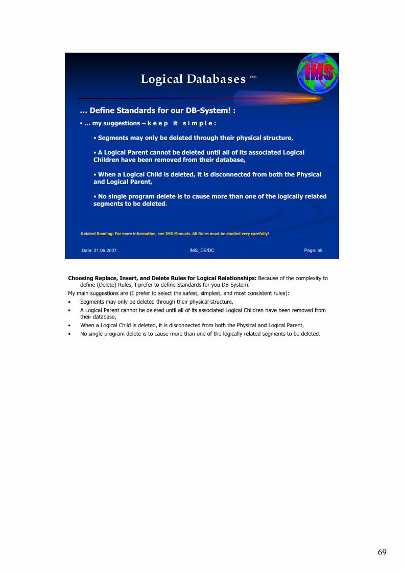
69
IMS_DB/DC Page: 69Date: 21.06.2007
Logical Databases (20)
… Define Standards for our DB-System! :
• … my suggestions – k e e p it s i m p l e :
• Segments may only be deleted through their physical structure,
• A Logical Parent cannot be deleted until all of its associated Logical Children have been removed from their database,
• When a Logical Child is deleted, it is disconnected from both the Physical and Logical Parent,
• No single program delete is to cause more than one of the logically related segments to be deleted.
Related Reading: For more information, see IMS Manuals. All Rules must be studied very carefully!
Choosing Replace, Insert, and Delete Rules for Logical Relationships: Because of the complexity to define (Delete) Rules, I prefer to define Standards for you DB-System.
My main suggestions are (I prefer to select the safest, simplest, and most consistent rules):
• Segments may only be deleted through their physical structure,
• A Logical Parent cannot be deleted until all of its associated Logical Children have been removed from their database,
• When a Logical Child is deleted, it is disconnected from both the Physical and Logical Parent,
• No single program delete is to cause more than one of the logically related segments to be deleted.
70
IMS_DB/DC Page: 70Date: 21.06.2007
Agenda Session 4: Logical Relationships /Logical Databases
1. Logical Relationships
2. Implementation Methods
• Unidirectional Relationship
• Bidirectional physically paired logical Relationships
• Bidirectional virtually paired logical Relationships
3. Paths in Logical Relationships
4. Logical Databases
5. Closing Comments
5. Closing Comments.

71
IMS_DB/DC Page: 71Date: 21.06.2007
Closing Comments
• Logical Relationships allow to view separate physical databasesas a single interrelated data structure,
• It is unfortunate that this most attractive capability is also the most complex and most frequently misused IMS option!
• With intelligent and skillful use, logical relationships can usually provide the interrelationship of data, between separate physicaldatabases, in a flexible and efficient manner.
Closing Comments:
Logical Relationships allow to view separate physical databases as a single interrelated data structure. This is, of course, the ultimate goal of “Data Management”.
It is unfortunate that this most attractive capability is also the most complex and most frequently misused IMS option! Perhaps the reason lies in the inherent complexity of the problem, in the hierarchical concept itself, or in the method chosen for providing the capability.
With intelligent and skillful use, logical relationships can usually provide the interrelationship of data, between separate physical databases, in a flexible and efficient manner. The challenge to the designer is to recognize the characteristics of the system and the functions which can efficiently use the logical relationship capability, in general, and the available options, in particular.

72
IMS_DB/DC Page: 72Date: 21.06.2007
Source
See: • IBM Web page
http://www-306.ibm.com/software/data/ims/
• BookAn Introduction to IMS, IBM Press
In all sessions I like to motivate you to study additional books and publications about IMS DB/DC.

73
Date: 21.06.2007 IMS_03_4.ppt Page: 73
Questions / CommentsQuestions / Comments……
? ? ?? ? ?
Questions, comments, further information?
Please feel free to e-mail me!
Dipl.Ing. Werner HoffmannDipl.Ing. Werner Hoffmann
EMAIL: EMAIL: pwhoffmann@[email protected]
The time for this session is over. If you have additional questions or comments or like to get further information please feel free to e mail me at [email protected] or [email protected]..

74
IMS_DB/DC Page: 74Date: 21.06.2007
The End…
Part III/4: IMS Hierarchical Database ModelIMS Hierarchical Database Model
Logical Databases /Logical RelationshipsLogical Databases /Logical Relationships
Workshop
The world depends on it
I hope this presentation was right for you! Enjoy the following discussion!
1
Date: 21.06.2007 IMS_03_5.ppt Page: 1
IBM Mainframe
IMS DB/DC
Database Design Workshop
Part III: Part III:
IMS Hierarchical Database ModelIMS Hierarchical Database ModelSession 5: Session 5: Indexed DatabasesIndexed Databases
April 2007 April 2007 –– 1st Version1st Version
presented bypresented by
Dipl. Dipl. IngIng. Werner Hoffmann. Werner HoffmannEMAIL: EMAIL: pwhoffmann @ tpwhoffmann @ t--online.deonline.de
A member of IEEE and ACM
Mainframe
Please see the notes pages for additional comments. Please see the notes pages for additional comments.
Welcome to the workshop called “IMS DB/DC". This is part III: IMS Hierarchical Database Model – Session 5: Indexed Databases.
2
IMS_DB/DC Page: 2Date: 21.06.2007
Agenda Session 5: Indexed Databases
1. Basics
2. Using Secondary Indexes with Logical Relationships
3. Using Secondary Indexes with Variable-Length Segments
4. Considerations When Using Secondary Indexing
5. Comparison to Logical Relationships
6. Summary
Here is the Agenda for the IMS DB/DC workshop part III/5: Indexed Databases.
In this session I like to speak about:
1. Basics
2. Using Secondary Indexes with Logical Relationships
3. Using Secondary Indexes with Variable-Length Segments
4. Considerations When Using Secondary Indexing
5. Comparison to Logical Relationships
6. Summary.

3
IMS_DB/DC Page: 3Date: 21.06.2007
Agenda Session 5: Indexed Databases
1. Basics2. Using Secondary Indexes with Logical
Relationships 3. Using Secondary Indexes with Variable-
Length Segments 4. Considerations When Using Secondary
Indexing 5. Comparison to Logical Relationships6. Summary
1. Basic Terms

4
IMS_DB/DC Page: 4Date: 21.06.2007
Secondary Indexes (1)
Basics
The following database types support secondary indexes:
• HISAM • HDAM • PHDAM • HIDAM • PHIDAM
• Characteristic:• Own separate Database (VSAM)• … are (invisible) to the application program.
Secondary Indexes: The following database types support secondary indexes:
• HISAM
• HDAM
• PHDAM
• HIDAM
• PHIDAM
Secondary indexes are indexes that allow you to process a segment type in a sequence other than the one defined by the segment’s key. A secondary index can also be used to process a segment type based on a qualification in a dependent segment.
Characteristics of Secondary Indexes: Secondary indexes can be used with HISAM, HDAM, PHDAM, HIDAM, and PHIDAM databases. A secondary index is in its own separate database and must use VSAM as its access method.
Secondary indexes are invisible to the application program. When an application program needs to do processing using the secondary index, this fact is communicated to IMS by coding the PROCSEQ= parameter in the PCB. If an application program needs to do processing using the regular processing sequence, PROCSEQ= is simply not coded. If the application program needs to do processing using both the regular processing sequence and the secondary index, the application program’s PSB must contain two PCBs, one with PROCSEQ= coded and one without. When two PCBs are used, it enables an application program to use two paths into the database and two sequence fields. One path and sequence field is provided by the regular processing sequence, and one is provided by the secondary index. The secondary index gives an application program both an alternative way to enter the database and an alternative way to sequentially process database records.

5
IMS_DB/DC Page: 5Date: 21.06.2007
Secondary Indexes (2)
Basics
Why Secondary Indexes?
• … segment ordering of a database• Keys
• Secondary Index• different processing requirements,• … alternate sequence,• … based on any field in the database.
Why Secondary Indexes? When you design your database records, you design them to meet the processing requirements of many applications. You decide what segments will be in a database record and what fields will be in a segment. You decide the order of segments in a database record and fields within a segment. You also decide which field in the root segment will be the key field, and whether the key field will be unique. All these decisions are based on what works best for all your application’s processing requirements. However, the choices you make might suit the processing requirements of some applications better than others.
Another application would be to access those segments by an alternate sequence. In this situation, you can use a secondary index that allows access to the database in e.g. course name sequence (rather than e.g. by course number, which is the key field). Secondary indexing is a solution to the different processing requirements of various applications. It allows you to have an index based on any field in the database, and not just the key field in the root segment.
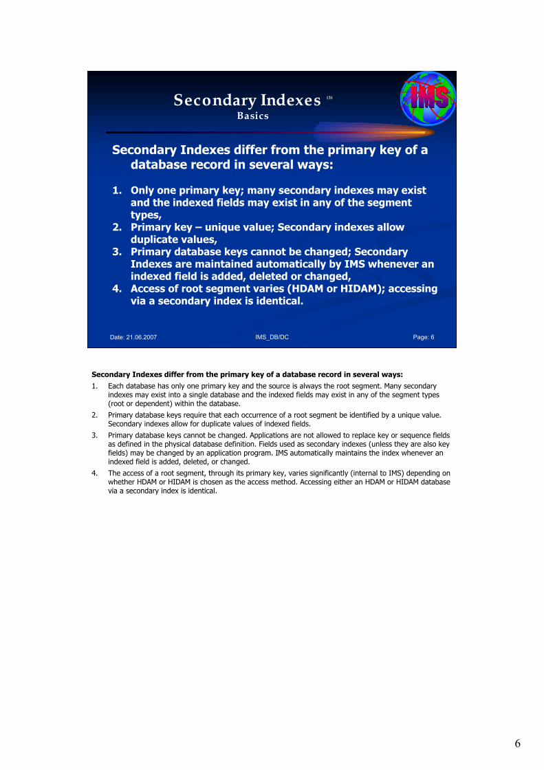
6
IMS_DB/DC Page: 6Date: 21.06.2007
Secondary Indexes (3)
Basics
Secondary Indexes differ from the primary key of a database record in several ways:
1. Only one primary key; many secondary indexes may exist and the indexed fields may exist in any of the segment types,
2. Primary key – unique value; Secondary indexes allow duplicate values,
3. Primary database keys cannot be changed; Secondary Indexes are maintained automatically by IMS whenever an indexed field is added, deleted or changed,
4. Access of root segment varies (HDAM or HIDAM); accessing via a secondary index is identical.
Secondary Indexes differ from the primary key of a database record in several ways:
1. Each database has only one primary key and the source is always the root segment. Many secondary indexes may exist into a single database and the indexed fields may exist in any of the segment types (root or dependent) within the database.
2. Primary database keys require that each occurrence of a root segment be identified by a unique value. Secondary indexes allow for duplicate values of indexed fields.
3. Primary database keys cannot be changed. Applications are not allowed to replace key or sequence fields as defined in the physical database definition. Fields used as secondary indexes (unless they are also key fields) may be changed by an application program. IMS automatically maintains the index whenever an indexed field is added, deleted, or changed.
4. The access of a root segment, through its primary key, varies significantly (internal to IMS) depending on whether HDAM or HIDAM is chosen as the access method. Accessing either an HDAM or HIDAM database via a secondary index is identical.
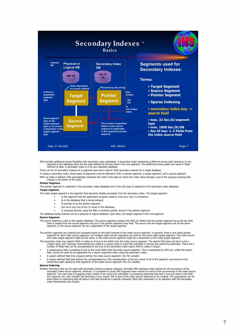
7
IMS_DB/DC Page: 7Date: 21.06.2007
Secondary Indexes (4)
Basics
Segments used for
Secondary Indexes:
Terms:
• Target Segment• Source Segment• Pointer Segment
• Sparse Indexing
• secondary index key -> search field
• max. 32 Sec.IX/segment type• max. 1000 Sec.IX/DB• Sec.IX key: 1..5 fields from the index source field
Pointer
Segment
Secondary Index
DB
Sec.IX
DB
Ordered by Sec.IX key
Key:
Unique
/SX
/CX
or
not unique
value
Target
Segment
Source
Segment
A Root or
dependent
segment
type
Same segment
type as the
target segment
type or, as shown,
a dependent of the
target segment
type
Physical or
Logical DB
IMS DB
Order dependent
on access method
Indexed
DB
The content of specified
fields in each source
segment is duplicated
in the respective pointer
segment.
IMS provides additional access flexibility with secondary index databases. A secondary index represents a different access path (pointers) to any segment in the database other tha the path defined by the key field in the root segment. The additional access paths can result in faster retrieval of data. A secondary index is in its own separate database.
There can be 32 secondary indexes for a segment type and a total of 1000 secondary indexes for a single database.
To setup a secondary index, three types of segments must be defined to IMS: a pointer segment, a target segment, and a source segment.
After an index is defined, IMS automatically maintains the index if the data on which the index relies changes, even if the program causing that change is not aware of the index.
Pointer Segment.
The pointer segment is contained in the secondary index database and is the only type of segment in the secondary index database.
Target segment.
The index target segment is the segment that becomes initially accessible from the secondary index. The target segment:
• Is the segment that the application program needs to view as a root in a hierarchy.
• Is in the database that is being indexed.
• Is pointed to by the pointer segment.
• Can be at any one of the 15 levels in the database.
• Is accessed directly using the RBA or symbolic pointer stored in the pointer segment.
The database being indexed can be a physical or logical database. Quit often, the target segment is the root segment.
Source Segment.
The source segment is also in the regular database. The source segment contains the field (or fields) that the pointer segment has as its key field. Data is copied from the source segment and put in the pointer segment’s key field. The source and the target segment can be the same segment, or the source segment can be a dependent of the target segment.
The pointer segments are ordered and accessed based on the field contents of the index source segment. In general, there is one index pointer segment for each index source segment, but multiple index pointer segments can point to the same index target segment. The index source and index target segment might be the same, or the index source segment might be a dependent of the index target segment.
The secondary index key (search field) is made up of one to five fields from the index source segment. The search field does not have to be a unique value, but I strongly recommends you make it a unique value to avoid the overhead in storing and searching duplicates. There are a number of fields that can be concatenated to the end of the secondary index search field to make it unique:
• A subsequence field, consisting of one to five more fields from the index source segment. This is maintained by IMS but, unlike the search field, cannot be used by an application for a search argument when using the secondary index.
• A system defined field that uniquely defines the index source segment: the /SX variable.
• A system defined field that defines the concatenated key (the concatenation of the key values of all of the segment occurrences in the hierarchical path leading to that segment) of the index source segment: the /CX variable.
Sparse Indexing.
Another technique that can be used with secondary indexes is sparse indexing. Normally IMS maintains index entries for all occurrences of the secondary index source segment. However, it is possible to cause IMS suppress index entries for some of the occurrences of the index source segment. You may want to suppress index entries if you were only interested in processing segments that had a non-null value in the field. As a general rule, only consider this technique if you expect 205 or less of the index source segments to be created. The suppression can be done either by specifying that all bytes in the field should be a specific character (NULLVAL parameter) or by selection with the Secondary index Maintenance exit routine.
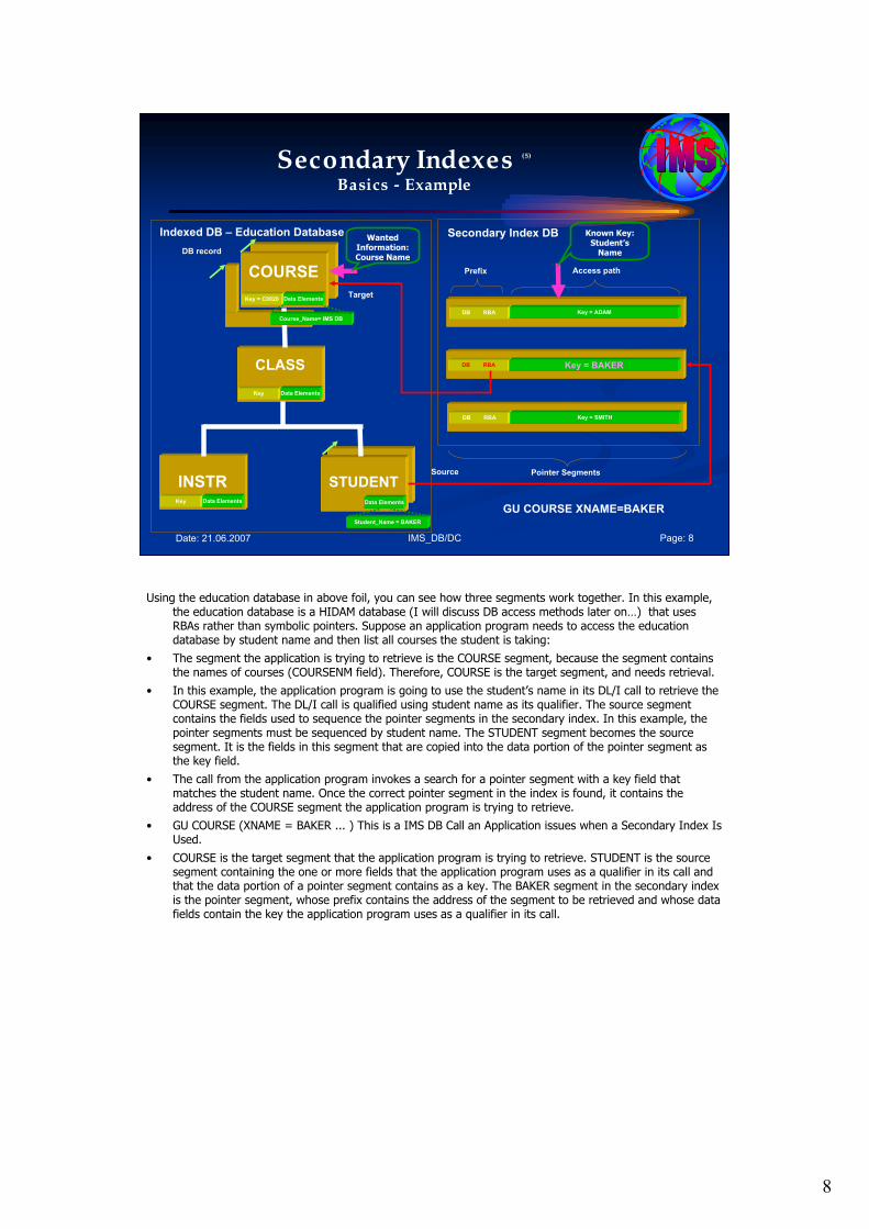
8
IMS_DB/DC Page: 8Date: 21.06.2007
Secondary Indexes (5)
Basics - Example
GU COURSE XNAME=BAKERKey= S0222
Prefix
DB RBA Key = ADAM
DB RBA Key = BAKER
DB RBA Key = SMITH
Pointer Segments
Secondary Index DB
Access pathCOURSE
CLASS
INSTR STUDENT
Indexed DB – Education Database
DB record
Key = C0020 Data Elements
Key Data Elements
Key Data Elements Data Elements
Known Key:Student’s Name
Wanted Information:Course Name
Course_Name= IMS DB
Target
Source
Student_Name = BAKER
Using the education database in above foil, you can see how three segments work together. In this example, the education database is a HIDAM database (I will discuss DB access methods later on…) that uses RBAs rather than symbolic pointers. Suppose an application program needs to access the education database by student name and then list all courses the student is taking:
• The segment the application is trying to retrieve is the COURSE segment, because the segment contains the names of courses (COURSENM field). Therefore, COURSE is the target segment, and needs retrieval.
• In this example, the application program is going to use the student’s name in its DL/I call to retrieve the COURSE segment. The DL/I call is qualified using student name as its qualifier. The source segment contains the fields used to sequence the pointer segments in the secondary index. In this example, the pointer segments must be sequenced by student name. The STUDENT segment becomes the source segment. It is the fields in this segment that are copied into the data portion of the pointer segment as the key field.
• The call from the application program invokes a search for a pointer segment with a key field that matches the student name. Once the correct pointer segment in the index is found, it contains the address of the COURSE segment the application program is trying to retrieve.
• GU COURSE (XNAME = BAKER ... ) This is a IMS DB Call an Application issues when a Secondary Index Is Used.
• COURSE is the target segment that the application program is trying to retrieve. STUDENT is the source segment containing the one or more fields that the application program uses as a qualifier in its call and that the data portion of a pointer segment contains as a key. The BAKER segment in the secondary index is the pointer segment, whose prefix contains the address of the segment to be retrieved and whose data fields contain the key the application program uses as a qualifier in its call.
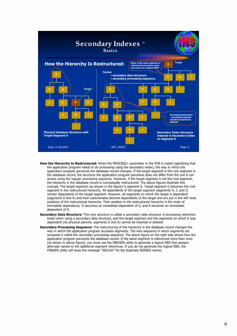
9
IMS_DB/DC Page: 9Date: 21.06.2007
Secondary Indexes (6)
Basics
How the Hierarchy Is Restructured:
A
B D
C E G K
F H J
I
Target
Physical Database Structure with Target Segment G
HD
G
J
Target
IG K
H J
I
E
F
A
B D
C E G K
F H J
I
Secondary Index Structure Indexed in Secondary Index on Segment G
Terms:• secondary data structure,• secondary processing sequence.
Processing Restriction:…its physical parents cannot be inserted or deleted!
Note: If the same segment is referenced more than once), you must use a logical DBD!
How the Hierarchy Is Restructured: When the PROCSEQ= parameter in the PCB is coded (specifying thatthe application program needs to do processing using the secondary index), the way in which the application program perceives the database record changes. If the target segment is the root segment in the database record, the structure the application program perceives does not differ from the one it can access using the regular processing sequence. However, if the target segment is not the root segment, the hierarchy in the database record is conceptually restructured. The above figures illustrate this concept. The target segment (as shown in the figure) is segment G. Target segment G becomes the root segment in the restructured hierarchy. All dependents of the target segment (segments H, J, and I) remain dependents of the target segment. However, all segments on which the target is dependent (segments D and A) and their subordinates become dependents of the target and are put in the left most positions of the restructured hierarchy. Their position in the restructured hierarchy is the order of immediate dependency. D becomes an immediate dependent of G, and A becomes an immediate dependent of D.
Secondary Data Structure: This new structure is called a secondary data structure. A processing restriction exists when using a secondary data structure, and the target segment and the segments on which it was dependent (its physical parents, segments D and A) cannot be inserted or deleted.
Secondary Processing Sequence: The restructuring of the hierarchy in the database record changes the way in which the application program accesses segments. The new sequence in which segments are accessed is called the secondary processing sequence. The above figure on the right side shows how the application program perceives the database record. If the same segment is referenced more than once (as shown in above figure), you must use the DBDGEN utility to generate a logical DBD that assigns alternate names to the additional segment references. If you do not generate the logical DBD, the PSBGEN utility will issue the message “SEG150” for the duplicate SENSEG names.
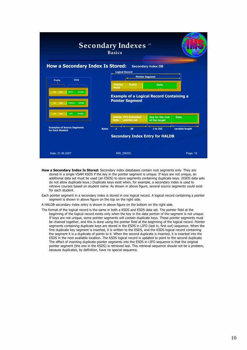
10
IMS_DB/DC Page: 10Date: 21.06.2007
Secondary Indexes (7)
Basics
How a Secondary Index Is Stored: Secondary Index DB
Prefix
DB RBA MATH ADAMS
Data
DB RBA FRENCH ADAMS
DB RBA HIST ADAMS
Examples of Source Segments for Each Student
Pointer PrefixField
Data
Logical Record
Bytes 1 28 1 to 255 variable length
Example of a Logical Record Containing a Pointer Segment
Delete EPS-ExtendedByte pointer set
Key for the root Dataof the target
Pointer Segment
Secondary Index Entry for HALDB
How a Secondary Index Is Stored: Secondary index databases contain root segments only. They are stored in a single VSAM KSDS if the key in the pointer segment is unique. If keys are not unique, an additional data set must be used (an ESDS) to store segments containing duplicate keys. (KSDS data sets do not allow duplicate keys.) Duplicate keys exist when, for example, a secondary index is used to retrieve courses based on student name. As shown in above figure, several source segments could exist for each student.
Each pointer segment in a secondary index is stored in one logical record. A logical record containing a pointer segment is shown in above figure on the top on the right side.
A HALDB secondary index entry is shown in above figure on the bottom on the right side.
The format of the logical record is the same in both a KSDS and ESDS data set. The pointer field at the beginning of the logical record exists only when the key in the data portion of the segment is not unique. If keys are not unique, some pointer segments will contain duplicate keys. These pointer segments must be chained together, and this is done using the pointer field at the beginning of the logical record. Pointer segments containing duplicate keys are stored in the ESDS in LIFO (last in, first out) sequence. When the first duplicate key segment is inserted, it is written to the ESDS, and the KSDS logical record containing the segment it is a duplicate of points to it. When the second duplicate is inserted, it is inserted into the ESDS in the next available location. The KSDS logical record is updated to point to the second duplicate. The effect of inserting duplicate pointer segments into the ESDS in LIFO sequence is that the original pointer segment (the one in the KSDS) is retrieved last. This retrieval sequence should not be a problem, because duplicates, by definition, have no special sequence.

11
IMS_DB/DC Page: 11Date: 21.06.2007
Secondary Indexes (8)
Basics
Format and Use of Fields in a Pointer Segment:
Examples of Several Source Segments for Each Student
Bytes 1 4 1 varies
Delete PointerByte field (RBA)
ConstantField (opt.)
SearchField (opt.)
Duplicate dataField (opt.)
CK-Filed (Opt.Except for HISAM
User Data(opt.)
Prefix Data
Terms:
• Delete Byte• Pointer Field• Constant Field• Search Field• Subsequence Field• Duplicate Data Field• Concatenated Key Field• User Data in Pointer Segment
Format and Use of Fields in a Pointer Segment: This topic contains diagnosis, modification, or tuning information.
The above figure shows the fields in a pointer segment. Like all segments, the pointer segment has a prefix and data portion. The prefix portion has a delete byte, and when direct rather than symbolic pointing is used, it has the address of the target segment (4 bytes). The data portion has a series of fields, and some of them are optional. All fields in the data portion of a pointer segment contain data taken from the source segment (with the exception of user data). These fields are the constant field (optional), the search field, the subsequence field (optional), the duplicate data field (optional), the concatenated key field (optional except for HISAM), and then the data (optional).
Delete Byte: The delete byte is used by IMS to determine whether a segment has been deleted from the database.
Pointer Field: This field, when present, contains the RBA of the target segment. The pointer field exists when direct pointing is specified for an index pointing to an HD database. Direct pointing is simply pointing to a segment using its actual address. The other type of pointing that can be specified is symbolic pointing. Symbolic pointing, which is explained under “Concatenated Key Field,” can be used to point to HD databases and must be used to point to HISAM databases. If symbolic pointing is used, this field does not exist.
Constant Field: This field, when present, contains a 1-byte constant. The constant is used when more than one index is put in an index database. The constant identifies all pointer segments for a specific index in the shared index database. The value in the constant field becomes part of the key.
Search Field: The data in the search field is the key of the pointer segment. All data in the search field comes from data in the source segment. As many as five fields from the source segment can be put in the search field. These fields do not need to be contiguous fields in the source segment. When the fields are stored in the pointer segment, they can be stored in any order. When stored, the fields are concatenated. The data in the search field (the key) can be unique or non-unique. IMS automatically maintains the search field in the pointer segment whenever a source segment is modified.
Subsequence Field: The subsequence field, like the search field, contains from one to five fields of data from the source segment. Subsequence fields are optional, and can be used if you have non-unique keys. The subsequence field can make non-unique keys unique. Making non-unique keys unique is desirable because of the many disadvantages of non-unique keys. For example, non-unique keys require you to use an additional data set, an ESDS, to store all index segments with duplicate keys. An ESDS requires additional space. More important, the search for specific occurrences of duplicates requires additional I/O operations that can decrease performance. When a subsequence field is used, the subsequence data is concatenated with the data in the search field. These concatenated fields become the key of the pointer segment. If properly chosen, the concatenated fields form a unique key. (It is not always possible to form a unique key using source data in the subsequence field. Therefore, you can use system related fields, explained later in the chapter, to form unique keys.) One important thing to note about using subsequence fields is that if you use them, the way in which an SSA is coded does not need to change. The SSA can still specify what is in the search field, but it cannot specify what is in the search plus the subsequence field. Subsequence fields are not seen by the application program unless it is processing the secondary index as a separate database. Up to five fields from the source segment can be put in the subsequence field. These fields do not need to be contiguous fields in the source segment. When the fields are stored in the pointer segment, they can be stored in any order. When stored, they are concatenated. IMS automatically maintains the subsequence field in the pointer segment whenever a source segment is modified.
Duplicate Data Field: The duplicate data field, like the search field, contains from one to five fields of data from the source segment. Duplicate data fields are optional. Use duplicate data fields when you have applications that process the secondary index as a separate database. Like the subsequence field, the duplicate data field is not seen by an application program unless it is processing the secondary index as a separate database. As many as five fields from the source segment can be put in the duplicate data field. These fields do not need to be contiguous fields in the source segment. When the fields are stored in the pointer segment, they can be stored in any order. When stored, they are concatenated. IMS automatically maintains the duplicate data field in the pointer segment whenever a source segment is modified.
Concatenated Key Field This field, when present, contains the concatenated key of the target segment. This field exists when the pointer segment points to the target segment symbolically, rather than directly. Direct pointing is simply pointing to a segment using its actual address. Symbolic pointing is pointing to a segment by a means other than its actual address. In a secondary index, the concatenated key of the target segment is used as a symbolic pointer. Segments in an HDAM or a HIDAM database being accessed using a secondary index can be accessed using a symbolic pointer. Segments in a HISAM database must be accessed using a symbolic pointer because segments in a HISAM database can “move around,” and the maintenance of direct-address pointers could be a large task. One of the implications of using symbolic pointers is that the physical parents of the target segment must be accessed to get to the target segment. Because of this extra access, retrieval of target segments using symbolic pointing is not as fast as retrieval using direct pointing. Also, symbolic pointers generally require more space in the pointer segment. When symbolic pointers are used, the key of the target segment is generally more than 4 bytes long. IMS automatically generates the concatenated key field when symbolic pointing is specified. One situation exists in which symbolic pointing is specified and IMS does not automatically generate the concatenated key field. This situation is caused by specifying the system-related field /CK as a subsequence or duplicate data field in such a way that the concatenated key is fully contained. In this situation, the symbolic pointer portion of either the subsequence field or the duplicate data field is used.
User Data in Pointer Segments: You can include any user data in the data portion of a pointer segment by specifying a segment length long enough to hold it. You need user data when applications process the secondary index as a separate database. Like data in the subsequence and duplicate data fields, user data is never seen by an application program unless it is processing the secondary index as a separate database. You must initially load user data. You must also maintain it. During reorganization of a database that uses secondary indexes, the secondary index database is rebuilt by IMS. During this process, all user data in the pointer segment is lost.

12
IMS_DB/DC Page: 12Date: 21.06.2007
Secondary Indexes (9)
Basics
Making Keys Unique Using System Related Fields:
• Using the /SX Operand• Using the /CK Operand
COURSE
CLASS
INSTR STUDENT
Target
Source
Database Record Showing the Source and Target for Secondary Indexes
COURSECD CLASSNO SEQ
Bytes 15 3 3
Concatenated Key of the STUDENT Segment
Making Keys Unique Using System Related Fields: You have already seen why it is desirable to have unique keys in the secondary index. You have also seen one way to force unique keys using the subsequence field in the pointer segment. If use of the subsequence field to contain additional information from the source segment does not work for you, there are two other ways to force unique keys. Both are done using an operand in the FIELD statement of the source segment in the DBD. The FIELD statement defines fields within a segment type.
Using the /SX Operand: For HD databases, you can code a FIELD statement with a NAME field that starts with /SX. The /SX can be followed by any additional characters (up to five) that you need. When you use this operand, the system generates (during segment insertion) the RBA, or an 8-byte ILK for PHDAM or PHIDAM, of the source segment. The system also puts the RBA or ILK in the subsequent field in the pointer segment, thus ensuring that the key is unique. The FIELD statement in which /SX is coded is the FIELD statement defining fields in the source segment. The /SX value is not, however, put in the source segment. It is put in the pointer segment. When you use the /SX operand, the XDFLD statement in the DBD must also specify /SX (plus any of the additional characters added to the /SX operand). The XDFLD statement, among other things, identifies fields from the source segment that are to be put in the pointer segment. The /SX operand is specified in the SUBSEQ= operand in the XDFLD statement.
Using the /CK Operand: The other way to force unique keys is to code a FIELD statement with a NAME parameter that starts with /CK. When used as a subsequence field, /CK ensures unique keys for pointer segments. You can use this operand for HISAM, HDAM, PHDAM, HIDAM, or PHIDAM databases. The /CK can be followed by up to five additional characters. The /CK operand works like the /SX operand except that the concatenated key, rather than the RBA, of the source segment is used. Another difference is that the concatenated key is put in the subsequence or duplicate data field in the pointer segment. Where the concatenated key is put depends on where you specify the /CK. When using /CK, you can use a portion of the concatenated key of the source segment (if some portion will make the key unique) or all of the concatenated key. You use the BYTES= and START= operands in the FIELD statement to specify what you need. For example, suppose you are using the database record shown in above figure.
If you specify on the FIELD statement whose name begins with /CK BYTES=21, START=1, the entire concatenated key of the source segment will be put in the pointer segment. If you specify BYTES=6, START=16, only the last six bytes of the concatenated key (CLASSNO and SEQ) will be put in the pointer segment. The BYTES= operand tells the system how many bytes are to be taken from the concatenated key of the source segment in the PCB key feedback area. The START= operand tells the system the beginning position (relative to the beginning of the concatenated key) of the information that needs to be taken. As with the /SX operand, the XDFLD statement in the DBD must also specify /CK. To summarize: /SX and /CK fields can be included on the SUBSEQ= parameter of the XDFLD statement to make key fields unique. Making key fields unique avoids the overhead of using an ESDS to hold duplicate keys. The /CK field can also be specified on the DDATA= parameter of the XDFLD statement but the field will not become part of the key field. When making keys unique, unique sequence fields must be defined in the target segment type, if symbolic pointing is used Also, unique sequence fields must be defined in all segment types on which the target segment type is dependent (in the physical rather than restructured hierarchy in the database).

13
IMS_DB/DC Page: 13Date: 21.06.2007
Secondary Indexes (10)
Basics
Suppressing Index Entries - Sparse Indexing:
• Advantages of Sparse Indexing:
• … allows you to specify the conditions under which a pointer segment is suppressed,
• … reduces the size of the index,• … you do not need to generate unnecessary index entries.
• How to Specify a Sparse Index:• NULLVAL= Operand on the XDFLD in DBD,• index maintenance exit routine
Suppressing Index Entries - Sparse Indexing: When a source segment is loaded, inserted, or replaced in the database, DL/I automatically creates or maintains the pointer segment in the index. This happens automatically unless you have specified that you do not need certain pointer segments built. For example: suppose you have a secondary index for the education database at which you have been previously looking. STUDENT is the source segment, and COURSE is the target segment. You might need to create pointer segments for students only if they are associated with a certain customer number. This could be done using sparse indexing, a performance enhancement of secondary indexing. Advantages of Sparse Indexing: Sparse indexing allows you to specify the conditions under which a pointer segment is suppressed, not generated, and put in the index database. Sparse indexing has two advantages. The primary one is that it reduces the size of the index, saving space and decreasing maintenance of the index. By decreasing the size of the index, performance is improved. The second advantage is that you do not need to generate unnecessary index entries.
How to Specify a Sparse Index: Sparse indexing can be specified in two ways: v You can code a value in the NULLVAL= operand on the XDFLD statement in the DBD that equals the condition under which you do not need a pointer segment put in the index. You can put BLANK, ZERO, or any 1-byte value (for example, X'10', C'Z', 5, or B'00101101') in the NULLVAL= operand. – BLANK is the same as C ' ' or X'40' –ZERO is the same as X'00' but not C'0‘. When using the NULLVAL= operand, a pointer segment is suppressed if every byte of the source field has the value you used in the operand.
If the values you are allowed to code in the NULLVAL= operand do not work for you, you can create an index maintenance exit routine that determines the condition under which you do not need a pointer segment put in the index. If you create your own index maintenance exit routine, you code its name in the EXTRTN= operand on the XDFLD statement in the DBD. You can only have one index maintenance exit routine for each secondary index. This exit routine, however, can be a general purpose one that is used by more than one secondary index.
The exit routine must be consistent in determining whether a particular pointer segment needs to be put in the index. The exit routine cannot examine the same pointer segment at two different times but only mark it for suppression once. Also, user data cannot be used by your exit routine to determine whether a pointer segment is to be put in the index. When a pointer segment needs to be inserted into the index, your exit routine only sees the actual pointer segment just before insertion. When a pointer segment is being replaced or deleted, only a prototype of the pointer segment is seen by your exit routine. The prototype contains the contents of the constant, search, subsequence, and duplicate data fields, plus the symbolic pointer if there is one.

14
IMS_DB/DC Page: 14Date: 21.06.2007
Secondary Indexes (11)
Basics
How the Secondary Index Is Maintained:
• Inserting a source segment,
• Deleting a Source Segment,
• Replacing a Source Segment.
Completely maintained by IMS
How the Secondary Index Is Maintained: When a source segment is inserted, deleted, or replaced in the database, IMS keeps the index current regardless whether the application program performing the update uses the secondary index. The way in which IMS maintains the index depends on the operation being performed. Regardless of the operation, IMS always begins index maintenance by building a pointer segment from information in the source segment that is being inserted, deleted, or replaced. (This pointer segment is built but not yet put in the secondary index database.)
Inserting a Source Segment: When a source segment is inserted, DL/I determines whether the pointer segment needs to be suppressed. If the pointer segment needs to be suppressed, it is not put in the secondary index. If the pointer segment does not need to be suppressed, it is put in the secondary index.
Deleting a Source Segment: When a source segment is deleted, IMS determines whether the pointer segment is one that was suppressed. If so, IMS does not do any index maintenance. If the segment is one that was suppressed, there should not be a corresponding pointer segment in the index to delete. If the pointer segment is not one that was suppressed, IMS finds the matching pointer segment in the index and deletes it. Unless the segment contains a pointer to the ESDS data set, which can occur with a non-unique secondary index, the logical record containing the deleted pointer segment in a KSDS data set is erased.
Replacing a Source Segment: When a source segment is replaced, the pointer segment in the index might or might not be affected. The pointer segment in the index might need to be replaced, or it might need to be deleted. After replacement or deletion, a new pointer segment is inserted. On the other hand, the pointer segment might need no changes. IMS determines what needs to be done by comparing the pointer segment it built (the new one) with the matching pointer segment in the secondary index (the old one).
• If both the new and the old pointer segments need to be suppressed, IMS does not do anything (no pointer segment exists in the index).
• If the new pointer segment needs to be suppressed but the old one does not, then the old pointer segment is deleted from the index.
• If the new pointer segment does not need to be suppressed but the old pointer segment is suppressed, then the new pointer segment is inserted into the secondary index.
• If neither the new or the old segment needs to be suppressed and:
• If there is no change to the old pointer segment, IMS does not do anything.
• If the non-key data portion in the new pointer segment is different from the old one, the old pointer segment is replaced. User data in the index pointer segment is preserved when the pointer segment is replaced.
• If the key portion in the new pointer segment is different from the old one, the old pointer segment is deleted and the new pointer segment is inserted. User data is not preserved when the index pointer segment is deleted and a new one inserted.
If you reorganize your secondary index and it contains non-unique keys, the resulting pointer segment order can be unpredictable.
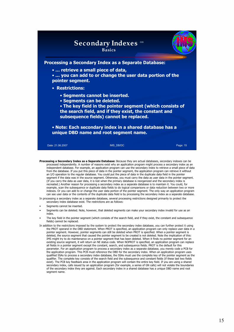
15
IMS_DB/DC Page: 15Date: 21.06.2007
Secondary Indexes (12)
Basics
Processing a Secondary Index as a Separate Database:
• … retrieve a small piece of data,• … you can add to or change the user data portion of the pointer segment.
• Restrictions:
• Segments cannot be inserted.• Segments can be deleted. • The key field in the pointer segment (which consists of the search field, and if they exist, the constant and subsequence fields) cannot be replaced.
• Note: Each secondary index in a shared database has a unique DBD name and root segment name.
Processing a Secondary Index as a Separate Database: Because they are actual databases, secondary indexes can be processed independently. A number of reasons exist why an application program might process a secondary index as an independent database. For example, an application program can use the secondary index to retrieve a small piece of data from the database. If you put this piece of data in the pointer segment, the application program can retrieve it without an I/O operation to the regular database. You could put the piece of data in the duplicate data field in the pointer segment if the data was in the source segment. Otherwise, you must carry the data as user data in the pointer segment. (If you carry the data as user data, it is lost when the primary database is reorganized and the secondary index is recreated.) Another reason for processing a secondary index as a separate database is to maintain it. You could, for example, scan the subsequence or duplicate data fields to do logical comparisons or data reduction between two or more indexes. Or you can add to or change the user data portion of the pointer segment. The only way an application program can see user data or the contents of the duplicate data field is by processing the secondary index as a separate database.
In processing a secondary index as a separate database, several processing restrictions designed primarily to protect the secondary index database exist. The restrictions are as follows:
• Segments cannot be inserted.
• Segments can be deleted. Note, however, that deleted segments can make your secondary index invalid for use as an index.
• The key field in the pointer segment (which consists of the search field, and if they exist, the constant and subsequence fields) cannot be replaced.
In addition to the restrictions imposed by the system to protect the secondary index database, you can further protect it using the PROT operand in the DBD statement. When PROT is specified, an application program can only replace user data in a pointer segment. However, pointer segments can still be deleted when PROT is specified. When a pointer segment is deleted, the source segment that caused the pointer segment to be created is not deleted. Note the implication of this: IMS might try to do maintenance on a pointer segment that has been deleted. When it finds no pointer segment for an existing source segment, it will return an NE status code. When NOPROT is specified, an application program can replace all fields in a pointer segment except the constant, search, and subsequence fields. PROT is the default for this parameter. For an application program to process a secondary index as a separate database, you merely code a PCB for the application program. This PCB must reference the DBD for the secondary index. When an application program uses qualified SSAs to process a secondary index database, the SSAs must use the complete key of the pointer segment as the qualifier. The complete key consists of the search field and the subsequence and constant fields (if these last two fields exist). The PCB key feedback area in the application program will contain the entire key field. If you are using a shared secondary index, calls issued by an application program (for example, a series of GN calls) will not violate the boundaries of the secondary index they are against. Each secondary index in a shared database has a unique DBD name and root segment name.

16
IMS_DB/DC Page: 16Date: 21.06.2007
Secondary Indexes (13)
Basics
Sharing Secondary Index Databases:
• max. 16 secondary indexes can be put in a single index database.
• Term: >1 secondary index -> shared index database
• HALDB does not support shared secondary indexes.
In a shared index database:
• All index segments must be the same length.
• All keys must be the same length.
• The offset from the beginning of all segments to the search field must be the same.
• Each shared secondary index requires a constant specified for it.
Sharing Secondary Index Databases: As many as 16 secondary indexes can be put in a single index database. When more than one secondary index is in the same database, the database is called a shared index database. HALDB does not support shared secondary indexes.
Although using a shared index database can save some main storage, the disadvantages of using a shared index database generally outweigh the small amount of space that is saved by its use. For example, performance can decrease when more than one application program simultaneously uses the shared index database. (Search time is increased because the arm must move back and forth between more than one secondary index.) In addition, maintenance, recovery, and reorganization of the shared index database can decrease performance because all secondary indexes are, to some extent, affected if one is. For example, when a database that is accessed using a secondary index is reorganized, IMS automatically builds a new secondary index. This means all other indexes in the shared database must be copied to the new shared index.
If you are using a shared index database, you need to know the following information:
• A shared index database is created, accessed, and maintained just like an index database with a single secondary index.
• The various secondary indexes in the shared index database do not need to index the same database.
• One shared index database could contain all secondary indexes for your installation (if the number of secondary indexes does not exceed 16).
In a shared index database:
• All index segments must be the same length.
• All keys must be the same length.
• The offset from the beginning of all segments to the search field must be the same. This means all keys must be either unique or non-unique. With non-unique keys, a pointer field exists in the target segment. With unique keys, it does not. So the offset to the key field, if unique and non-unique keys were mixed, would differ by 4 bytes. If the search fields in your secondary indexes are not the same length, you might be able to force key fields of equal length by using the subsequence field. You can put the number of bytes you need to make each key field an equal length in the subsequence field.
• Each shared secondary index requires a constant specified for it, a constant that uniquely identifies it from other indexes in the secondary index database. IMS puts this identifier in the constant field of each pointer segment in the secondary index database. For shared indexes, the key is the constant, search, and (if used) the subsequence field.

17
IMS_DB/DC Page: 17Date: 21.06.2007
Secondary Indexes (14)
Basics
PSINDEX
• Supported by DBCTL • Supports up to 1001 partitions • Partitions support only a single data set • Do not need to rebuild after reorganizations of the indexed database because of the HALDB self-healing pointer process • Partitions within the partitioned secondary index (PSINDEX) can be allocated, authorized, processed, reorganized, and recovered independently of the other partitions in the database • Segments have a larger prefix than non-partitioned secondary indexes to accommodate both a 28-byte extended pointer set (EPS) and the length of the root key of the secondary index target segment • Does not support shared secondary indexes • Does not support symbolic pointers • Requires the secondary index record segments to have unique keys
HALDB partitioned secondary index: PSINDEX
• Supported by DBCTL
• Supports up to 1001 partitions
• Partitions support only a single data set
• Do not need to rebuild after reorganizations of the indexed database because of the HALDB self-healing pointer process
• Partitions within the partitioned secondary index (PSINDEX) can be allocated, authorized, processed, reorganized, and recovered independently of the other partitions in the database
• Segments have a larger prefix than non-partitioned secondary indexes to accommodate both a 28-byte extended pointer set (EPS) and the length of the root key of the secondary index target segment
• Does not support shared secondary indexes
• Does not support symbolic pointers
• Requires the secondary index record segments to have unique keys

18
IMS_DB/DC Page: 18Date: 21.06.2007
Secondary Indexes (15)
Basics
PSINDEX
• Additionally, there are other requirements and considerations for HALDB partitioned secondary indexes:
• Secondary indexes must have unique keys. • /SX and /CK fields can be used to provide uniqueness. • The reorganization of a target database does not require the rebuilding of its secondary indexes. HALDBs use an indirect list data set (ILDS) to maintain pointers between the PSINDEX and the target segments.
HALDB partitioned secondary index: PSINDEX
• Additionally, there are other requirements and considerations for HALDB partitioned secondary indexes:
• Secondary indexes must have unique keys.
• /SX and /CK fields can be used to provide uniqueness.
• The reorganization of a target database does not require the rebuilding of its secondary indexes. HALDBs use an indirect list data set (ILDS) to maintain pointers between the PSINDEX and the target segments.
19
IMS_DB/DC Page: 19Date: 21.06.2007
Agenda Session 5: Indexed Databases
1. Basics
2. Using Secondary Indexes with Logical Relationships
3. Using Secondary Indexes with Variable-Length Segments
4. Considerations When Using Secondary Indexing
5. Comparison to Logical Relationships6. Summary
2. Using Secondary Indexes with Logical Relationships
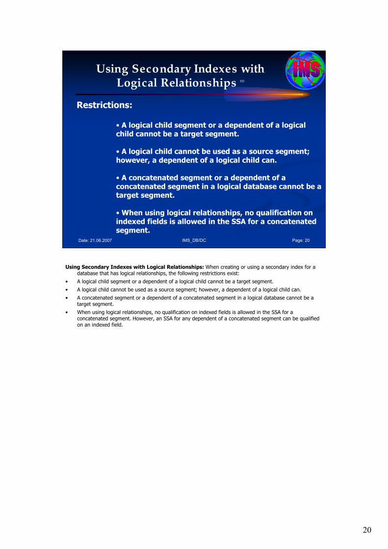
20
IMS_DB/DC Page: 20Date: 21.06.2007
Using Secondary Indexes with Logical Relationships (1)
Restrictions:
• A logical child segment or a dependent of a logical child cannot be a target segment.
• A logical child cannot be used as a source segment; however, a dependent of a logical child can.
• A concatenated segment or a dependent of a concatenated segment in a logical database cannot be a target segment.
• When using logical relationships, no qualification on indexed fields is allowed in the SSA for a concatenated segment.
Using Secondary Indexes with Logical Relationships: When creating or using a secondary index for a database that has logical relationships, the following restrictions exist:
• A logical child segment or a dependent of a logical child cannot be a target segment.
• A logical child cannot be used as a source segment; however, a dependent of a logical child can.
• A concatenated segment or a dependent of a concatenated segment in a logical database cannot be a target segment.
• When using logical relationships, no qualification on indexed fields is allowed in the SSA for a concatenated segment. However, an SSA for any dependent of a concatenated segment can be qualified on an indexed field.
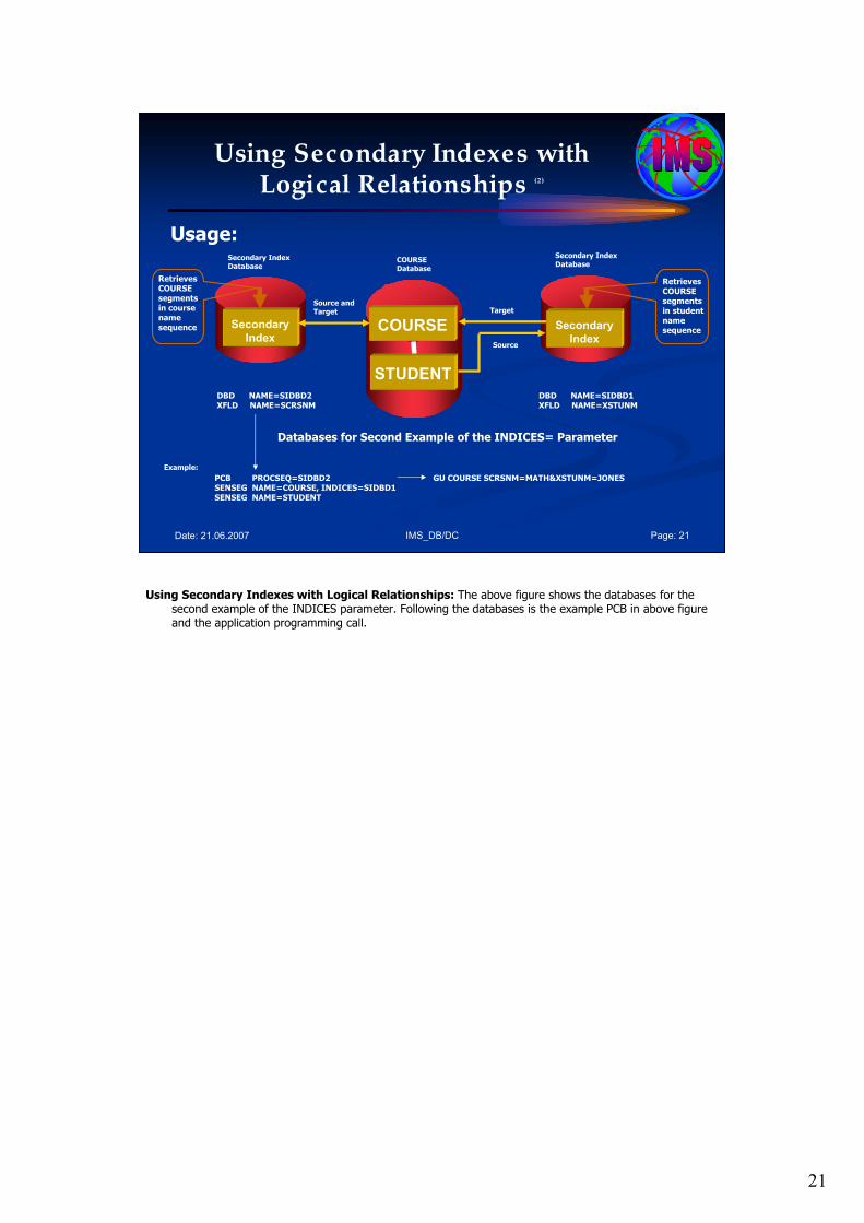
21
IMS_DB/DC Page: 21Date: 21.06.2007
Using Secondary Indexes with Logical Relationships (2)
Usage:
GU COURSE SCRSNM=MATH&XSTUNM=JONESPCB PROCSEQ=SIDBD2 SENSEG NAME=COURSE, INDICES=SIDBD1 SENSEG NAME=STUDENT
Example:
COURSE
STUDENT
Secondary
Index
Target
Source
Secondary IndexDatabase
Secondary IndexDatabase
COURSEDatabase
Secondary
Index
RetrievesCOURSEsegmentsin coursename sequence
RetrievesCOURSEsegmentsin studentname sequence
DBD NAME=SIDBD2XFLD NAME=SCRSNM
DBD NAME=SIDBD1XFLD NAME=XSTUNM
Databases for Second Example of the INDICES= Parameter
Source andTarget
Using Secondary Indexes with Logical Relationships: The above figure shows the databases for the second example of the INDICES parameter. Following the databases is the example PCB in above figure and the application programming call.
22
IMS_DB/DC Page: 22Date: 21.06.2007
Agenda Session 5: Indexed Databases
1. Basics2. Using Secondary Indexes with Logical
Relationships
3. Using Secondary Indexes with Variable-Length Segments
4. Considerations When Using Secondary Indexing
5. Comparison to Logical Relationships6. Summary
3. Using Secondary Indexes with Variable-Length Segments
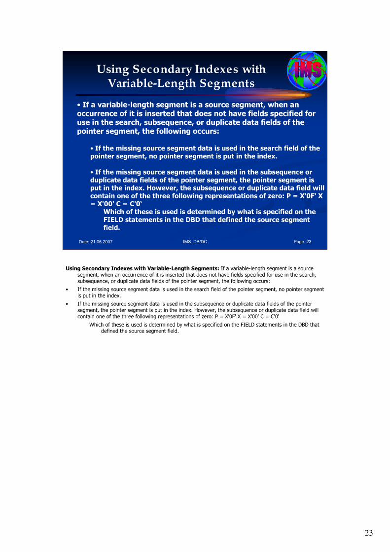
23
IMS_DB/DC Page: 23Date: 21.06.2007
Using Secondary Indexes with Variable-Length Segments
• If a variable-length segment is a source segment, when an occurrence of it is inserted that does not have fields specified for use in the search, subsequence, or duplicate data fields of the pointer segment, the following occurs:
• If the missing source segment data is used in the search field of the pointer segment, no pointer segment is put in the index.
• If the missing source segment data is used in the subsequence or duplicate data fields of the pointer segment, the pointer segment is put in the index. However, the subsequence or duplicate data field will contain one of the three following representations of zero: P = X'0F' X = X'00' C = C'0‘
Which of these is used is determined by what is specified on theFIELD statements in the DBD that defined the source segment field.
Using Secondary Indexes with Variable-Length Segments: If a variable-length segment is a source segment, when an occurrence of it is inserted that does not have fields specified for use in the search, subsequence, or duplicate data fields of the pointer segment, the following occurs:
• If the missing source segment data is used in the search field of the pointer segment, no pointer segment is put in the index.
• If the missing source segment data is used in the subsequence or duplicate data fields of the pointer segment, the pointer segment is put in the index. However, the subsequence or duplicate data field will contain one of the three following representations of zero: P = X'0F' X = X'00' C = C'0‘
Which of these is used is determined by what is specified on the FIELD statements in the DBD that defined the source segment field.

24
IMS_DB/DC Page: 24Date: 21.06.2007
Agenda Session 5: Indexed Databases
1. Basics2. Using Secondary Indexes with Logical
Relationships 3. Using Secondary Indexes with Variable-
Length Segments
4. Considerations When Using Secondary Indexing
5. Comparison to Logical Relationships6. Summary
4. Considerations When Using Secondary Indexing
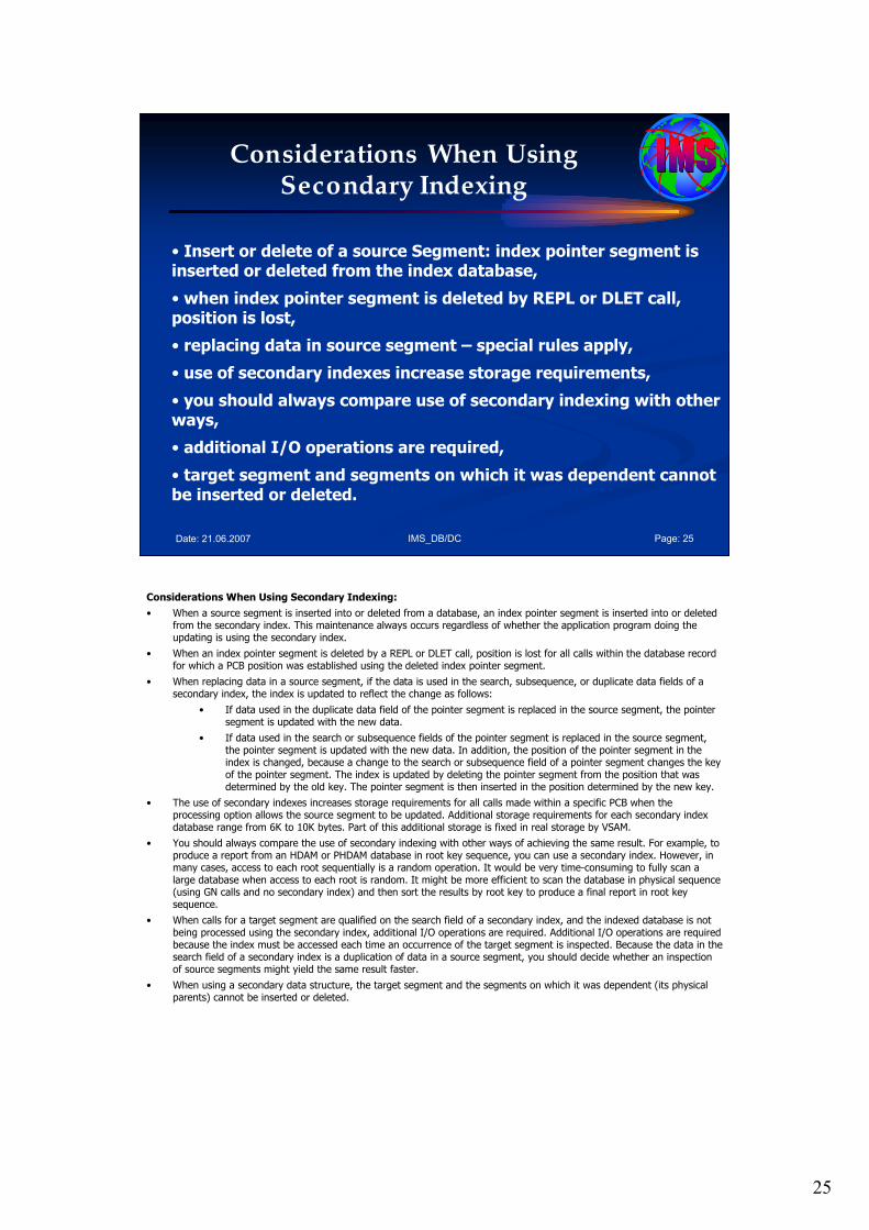
25
IMS_DB/DC Page: 25Date: 21.06.2007
Considerations When Using Secondary Indexing
• Insert or delete of a source Segment: index pointer segment is inserted or deleted from the index database,
• when index pointer segment is deleted by REPL or DLET call, position is lost,
• replacing data in source segment – special rules apply,
• use of secondary indexes increase storage requirements,
• you should always compare use of secondary indexing with other ways,
• additional I/O operations are required,
• target segment and segments on which it was dependent cannot be inserted or deleted.
Considerations When Using Secondary Indexing:
• When a source segment is inserted into or deleted from a database, an index pointer segment is inserted into or deleted from the secondary index. This maintenance always occurs regardless of whether the application program doing the updating is using the secondary index.
• When an index pointer segment is deleted by a REPL or DLET call, position is lost for all calls within the database record for which a PCB position was established using the deleted index pointer segment.
• When replacing data in a source segment, if the data is used in the search, subsequence, or duplicate data fields of a secondary index, the index is updated to reflect the change as follows:
• If data used in the duplicate data field of the pointer segment is replaced in the source segment, the pointer segment is updated with the new data.
• If data used in the search or subsequence fields of the pointer segment is replaced in the source segment, the pointer segment is updated with the new data. In addition, the position of the pointer segment in the index is changed, because a change to the search or subsequence field of a pointer segment changes the key of the pointer segment. The index is updated by deleting the pointer segment from the position that was determined by the old key. The pointer segment is then inserted in the position determined by the new key.
• The use of secondary indexes increases storage requirements for all calls made within a specific PCB when the processing option allows the source segment to be updated. Additional storage requirements for each secondary index database range from 6K to 10K bytes. Part of this additional storage is fixed in real storage by VSAM.
• You should always compare the use of secondary indexing with other ways of achieving the same result. For example, to produce a report from an HDAM or PHDAM database in root key sequence, you can use a secondary index. However, in many cases, access to each root sequentially is a random operation. It would be very time-consuming to fully scan a large database when access to each root is random. It might be more efficient to scan the database in physical sequence (using GN calls and no secondary index) and then sort the results by root key to produce a final report in root key sequence.
• When calls for a target segment are qualified on the search field of a secondary index, and the indexed database is not being processed using the secondary index, additional I/O operations are required. Additional I/O operations are required because the index must be accessed each time an occurrence of the target segment is inspected. Because the data in the search field of a secondary index is a duplication of data in a source segment, you should decide whether an inspection of source segments might yield the same result faster.
• When using a secondary data structure, the target segment and the segments on which it was dependent (its physical parents) cannot be inserted or deleted.
26
IMS_DB/DC Page: 26Date: 21.06.2007
Agenda Session 5: Indexed Databases
1. Basics2. Using Secondary Indexes with Logical
Relationships 3. Using Secondary Indexes with Variable-
Length Segments 4. Considerations When Using Secondary
Indexing
5. Comparison to Logical Relationships
6. Summary
5. Comparison to Logical Relationships
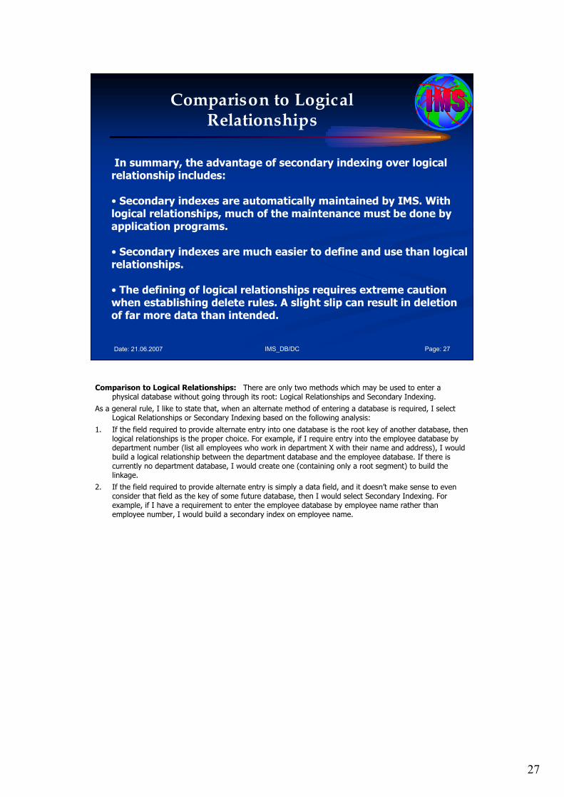
27
IMS_DB/DC Page: 27Date: 21.06.2007
Comparison to Logical Relationships
In summary, the advantage of secondary indexing over logical relationship includes:
• Secondary indexes are automatically maintained by IMS. With logical relationships, much of the maintenance must be done by application programs.
• Secondary indexes are much easier to define and use than logical relationships.
• The defining of logical relationships requires extreme caution when establishing delete rules. A slight slip can result in deletion of far more data than intended.
Comparison to Logical Relationships: There are only two methods which may be used to enter a physical database without going through its root: Logical Relationships and Secondary Indexing.
As a general rule, I like to state that, when an alternate method of entering a database is required, I select Logical Relationships or Secondary Indexing based on the following analysis:
1. If the field required to provide alternate entry into one database is the root key of another database, then logical relationships is the proper choice. For example, if I require entry into the employee database by department number (list all employees who work in department X with their name and address), I would build a logical relationship between the department database and the employee database. If there is currently no department database, I would create one (containing only a root segment) to build the linkage.
2. If the field required to provide alternate entry is simply a data field, and it doesn’t make sense to even consider that field as the key of some future database, then I would select Secondary Indexing. For example, if I have a requirement to enter the employee database by employee name rather than employee number, I would build a secondary index on employee name.
28
IMS_DB/DC Page: 28Date: 21.06.2007
Agenda Session 5: Indexed Databases
1. Basics2. Using Secondary Indexes with Logical
Relationships 3. Using Secondary Indexes with Variable-
Length Segments 4. Considerations When Using Secondary
Indexing 5. Comparison to Logical Relationships
6. Summary
6. Summary
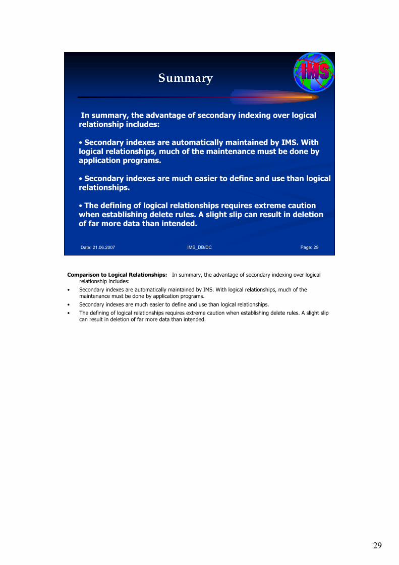
29
IMS_DB/DC Page: 29Date: 21.06.2007
Summary
In summary, the advantage of secondary indexing over logical relationship includes:
• Secondary indexes are automatically maintained by IMS. With logical relationships, much of the maintenance must be done by application programs.
• Secondary indexes are much easier to define and use than logical relationships.
• The defining of logical relationships requires extreme caution when establishing delete rules. A slight slip can result in deletion of far more data than intended.
Comparison to Logical Relationships: In summary, the advantage of secondary indexing over logical relationship includes:
• Secondary indexes are automatically maintained by IMS. With logical relationships, much of the maintenance must be done by application programs.
• Secondary indexes are much easier to define and use than logical relationships.
• The defining of logical relationships requires extreme caution when establishing delete rules. A slight slip can result in deletion of far more data than intended.
30
IMS_DB/DC Page: 30Date: 21.06.2007
Source
See: • IBM Web page
http://www-306.ibm.com/software/data/ims/
• BookAn Introduction to IMS, IBM Press
In all sessions I like to motivate you to study additional books and publications about IMS DB/DC.

31
Date: 21.06.2007 IMS_03_5.ppt Page: 31
Questions / CommentsQuestions / Comments……
? ? ?? ? ?
Questions, comments, further information?
Please feel free to e-mail me!
Dipl.Ing. Werner HoffmannDipl.Ing. Werner Hoffmann
EMAIL: EMAIL: pwhoffmann@[email protected]
The time for this session is over. If you have additional questions or comments or like to get further information please feel free to e mail me at [email protected] or [email protected].

32
IMS_DB/DC Page: 32Date: 21.06.2007
The End…
Part III/5: IMS Hierarchical Database ModelIMS Hierarchical Database Model
Indexed DatabasesIndexed Databases
Workshop
The world depends on it
I hope this presentation was right for you! Enjoy the following discussion!

1
Date: 21.06.2007 IMS_03_6.ppt Page: 1
IBM Mainframe
IMS DB/DC
Database Design Workshop
Part III: Part III:
IMS Hierarchical Database ModelIMS Hierarchical Database ModelSession 6: Session 6: Data Sharing IssuesData Sharing Issues
March 2007 March 2007 –– 1st Version1st Version
presented bypresented by
Dipl. Dipl. IngIng. Werner Hoffmann. Werner HoffmannEMAIL: EMAIL: pwhoffmann @ tpwhoffmann @ t--online.deonline.de
A member of IEEE and ACM
Mainframe
Please see the notes pages for additional comments. Please see the notes pages for additional comments.
Welcome to the workshop called “IMS DB/DC". This is part III: IMS Hierarchical Database Model – Session 6: Data Sharing Issues.
2
IMS_DB/DC Page: 2Date: 21.06.2007
Agenda Session 6: Data Sharing Issues
1. Integrity
2. Unit of Work
3. Commit Points / Sync Points
4. Locking
5. PROCOPTs
6. DL/I Calls
7. Deadlocks
8. Summary
Here is the Agenda for the IMS DB/DC workshop part III/6: Data Sharing Issues.
In this session I like to speak about:
1. Integrity
2. Unit of Work
3. Commit Points / Sync Points
4. Locking
5. PROCOPTs
6. DL/I Calls
7. Deadlocks
8. Summary
3
IMS_DB/DC Page: 3Date: 21.06.2007
Agenda Session 6: Data Sharing Issues
1. Integrity
2. Unit of Work
3. Commit Points / Sync Points
4. Locking
5. PROCOPTs
6. DL/I Calls
7. Deadlocks
8. Summary
1. Integrity
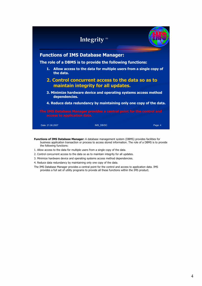
4
IMS_DB/DC Page: 4Date: 21.06.2007
Integrity (1)
Functions of IMS Database Manager:
The role of a DBMS is to provide the following functions:
1. Allow access to the data for multiple users from a single copy of the data.
2. Control concurrent access to the data so as to maintain integrity for all updates.
3. Minimize hardware device and operating systems access method dependencies.
4. Reduce data redundancy by maintaining only one copy of the data.
The IMS Database Manager provides a central point for the control and access to application data.
Functions of IMS Database Manager: A database management system (DBMS) provides facilities for business application transaction or process to access stored information. The role of a DBMS is to provide the following functions:
1. Allow access to the data for multiple users from a single copy of the data.
2. Control concurrent access to the data so as to maintain integrity for all updates.
3. Minimize hardware device and operating systems access method dependencies.
4. Reduce data redundancy by maintaining only one copy of the data.
The IMS Database Manager provides a central point for the control and access to application data. IMS provides a full set of utility programs to provide all these functions within the IMS product.
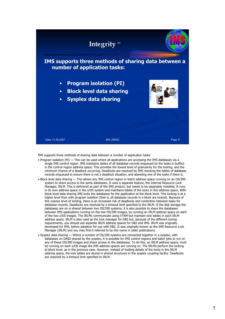
5
IMS_DB/DC Page: 5Date: 21.06.2007
Integrity (2)
IMS supports three methods of sharing data between a number of application tasks:
• Program isolation (PI)
• Block level data sharing
• Sysplex data sharing
IMS supports three methods of sharing data between a number of application tasks:
• Program isolation (PI) — This can be used where all applications are accessing the IMS databases via a single IMS control region. IMS maintains tables of all database records enqueued by the tasks in buffers in the control region address space. This provides the lowest level of granularity for the locking, and the minimum chance of a deadlock occurring. Deadlocks are resolved by IMS checking the tables of database records enqueued to ensure there is not a deadlock situation, and abending one of the tasks if there is.
• Block level data sharing — This allows any IMS control region or batch address space running on an OS/390 system to share access to the same databases. It uses a separate feature, the Internal Resource Lock Manager, IRLM. This is delivered as part of the IMS product, but needs to be separately installed. It runs in its own address space in the z/OS system and maintains tables of the locks in this address space. With block level data sharing IMS locks the databases for the application at the block level. This locking is at a higher level than with program isolation (that is, all database records in a block are locked). Because of this coarser level of locking, there is an increased risk of deadlocks and contention between tasks for database records. Deadlocks are resolved by a timeout limit specified to the IRLM. If the disk storage the databases are on is shared between two OS/390 systems, it is also possible to share the databases between IMS applications running on the two OS/390 images, by running an IRLM address space on each of the two z/OS images. The IRLMs communicate using VTAM but maintain lock tables in each IRLM address space. IRLM is also used as the lock manager for DB2 but, because of the different tuning requirements, you should use separate IRLM address spaces for DB2 and IMS. IRLM was originally developed for IMS, before adoption for use with DB2. It was originally known as the IMS Resource Lock Manager (IRLM) and you may find it referred to by this name in older publications.
• Sysplex data sharing — Where a number of OS/390 systems are connected together in a sysplex, with databases on DASD shared by the sysplex, it is possible for IMS control regions and batch jobs to run on any of these OS/390 images and share access to the databases. To do this, an IRLM address space, must be running on each z/OS image the IMS address spaces are running on. The IRLMs perform the locking at block level, as in the previous case. However, instead of holding details of the locks in the IRLM address space, the lock tables are stored in shared structures in the sysplex coupling facility. Deadlocks are resolved by a timeout limit specified to IRLM.
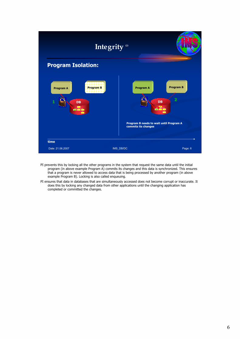
6
IMS_DB/DC Page: 6Date: 21.06.2007
Integrity (2)
Program Isolation:
time
1
Program A Program B
DB
xx
2
Program A Program B
DB
xx
Program B needs to wait until Program A commits its changes
PI prevents this by locking all the other programs in the system that request the same data until the initial program (in above example Program A) commits its changes and this data is synchronized. This ensures that a program is never allowed to access data that is being processed by another program (in above example Program B). Locking is also called enqueuing.
PI ensures that data in databases that are simultaneously accessed does not become corrupt or inaccurate. It does this by locking any changed data from other applications until the changing application has completed or committed the changes.
7
IMS_DB/DC Page: 7Date: 21.06.2007
Integrity (2)
Program isolation and dynamic logging:
… with program isolation• All activity of an application program is isolated from any other
application program(s)• Until an application program commits, by • Reaching a synchronization point.
• This ensures that only committed data can be used by concurrent application programs.
• A synchronization point is established with a GU call for a new input message and/or a checkpoint call, or normal program termination.
• Logging all DB images makes it possible to dynamic back out the effects of an application program that terminates abnormally.
Program isolation and dynamic logging: When processing DL/I database calls, the IMS program isolation function will ensure database integrity.
With program isolation, all activity (database modifications and message creation) of an application program is isolated from any other application program(s) running in the system until an application program commits, by reaching a synchronization point, the data it has modified or created. This ensures that only committed data can be used by concurrent application programs. A synchronization point in our subset is established with a get unique call for a new input message (single mode) and/or a checkpoint call (BMP only), or program normal termination (GOBACK or RETURN).
Program isolation allows two or more application programs to concurrently execute with common data segment types even when processing intent is segment update, add, or delete. This is done by a dynamic enqueue/dequeue routine which enqueues the affected database elements (segments, pointers, free space elements, etc.) between synchronization points. At the same time, the dynamic log modules log the prior database record images between those synchronization points. This makes it possible to dynamically back out the effects of an application program that terminates abnormally, without affecting the integrity of the databases controlled by IMS. It does not affect the activity of other application program(s) running concurrently in the system.
With program isolation and dynamic backout, it is possible to provide database segment occurrence level control to application programs. A means is provided for resolving possible deadlock situations in a manner transparent to the application program.
8
IMS_DB/DC Page: 8Date: 21.06.2007
Integrity (3)
Lock Management:
IMS uses locking to serialize processing. There are two prime reasons for this lock serialization:
1. It ensures that no application program can access uncommitted updates.
2. It serializes updates to a OSAM block or VSAM control interval.
Lock Management: IMS uses locking to serialize processing. There are two prime reasons for this lock serialization.
First, it ensures that no application program can access uncommitted updates.
Secondly, it serializes updates to a OSAM block or VSAM control interval.

9
IMS_DB/DC Page: 9Date: 21.06.2007
Integrity (4)
Lock Management:
• One IMS system:
• Full function databases use either the program isolation (PI) lock manager, or the IRLM,• Fast Path databases use the Fast Path lock manager in conjunction with either the program isolation lock manager or the IRLM,• locking is known as local locking.
• Data Sharing Sysplex:
• locking is extended across all IMS subsystems in the data sharing group,• IRLM is used (block-level data sharing),• locking is known as global locking.
Note: Internal Resource Lock Manager (IRLM)
Lock Management:
Without data sharing, locking is done for only one IMS system. Full function databases use either the program isolation (PI) lock manager, or the IRLM. Fast Path databases use the Fast Path lock manager in conjunction with either the program isolation lock manager or the IRLM. Knowledge of these locks does not have to be spread to other instances of these lock managers. Without data sharing, locking is known as local locking.
In the data sharing sysplex, locking is extended across all IMS subsystems in the data sharing group. This is known as global locking. Locks prevent the sharing subsystems from concurrently updating the same block or control interval (CI). The block or CI is locked before making the update and the lock is held until the buffer is written to DASD (and all other copies of the buffer have been invalidated in other subsystems if necessary), during sync point processing or buffer steal processing.
When a lock is requested, the request may not be compatible with a holder of the lock. This prevents the IRLM from granting the lock request. Typically, the requestor must wait until the holder releases the lock. On the other hand, locks can be requested with a conditional attribute. Conditional lock requests don't wait for release by holders; instead, the IRLM tells the requestor that the lock is not available. The requestor cannot have the lock and must take some other action.
With block level data sharing, the IRLM must be used. One IRLM can share locking information with other IRLM instances by means of a notification process. Notifications are messages sent from one IMS to other IMS systems in the data sharing group. These messages contain information that other IMS systems need. For example, when global commands are issued in one IMS system, notifications are sent to other IMS systems. Similarly, data set extension information is sent by notifications.
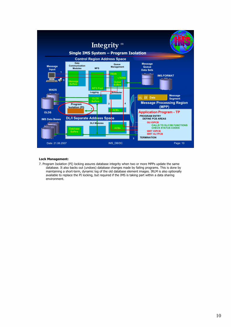
10
IMS_DB/DC Page: 10Date: 21.06.2007
Integrity (5)
Control Region Address Space
MessageBuffers
Data
Communication
Modules
Queue Management
Application Program - TPPROGRAM ENTRYDEFINE PCB AREAS
CALLS TO DL/I DB FUNCTIONSCHECK STATUS CODES
TERMINATION
MFS Pool
MFSMessage
Input
Message
Queue
Data Sets
IMS.FORMAT
OLDSBuffers
LoggingWADS
OLDS
Program
Isolation (PI)
Scheduler
ACBs
ACBsDatabase
Buffers
GU IOPCB
ISRT IOPCBISRT ALTPCB
DL/I Separate Address Space
Message Processing Region(MPP)
IMS Data Bases
DL/I Modules
LL ZZ Data Message
Segment
1
2
3
4
QueueBuffers
TRAN
LTERM5
7
Single IMS System – Program Isolation
Lock Management:
7. Program Isolation (PI) locking assures database integrity when two or more MPPs update the same database. It also backs out (undoes) database changes made by failing programs. This is done by maintaining a short-term, dynamic log of the old database element images. IRLM is also optionally available to replace the PI locking, but required if the IMS is taking part within a data sharing environment.
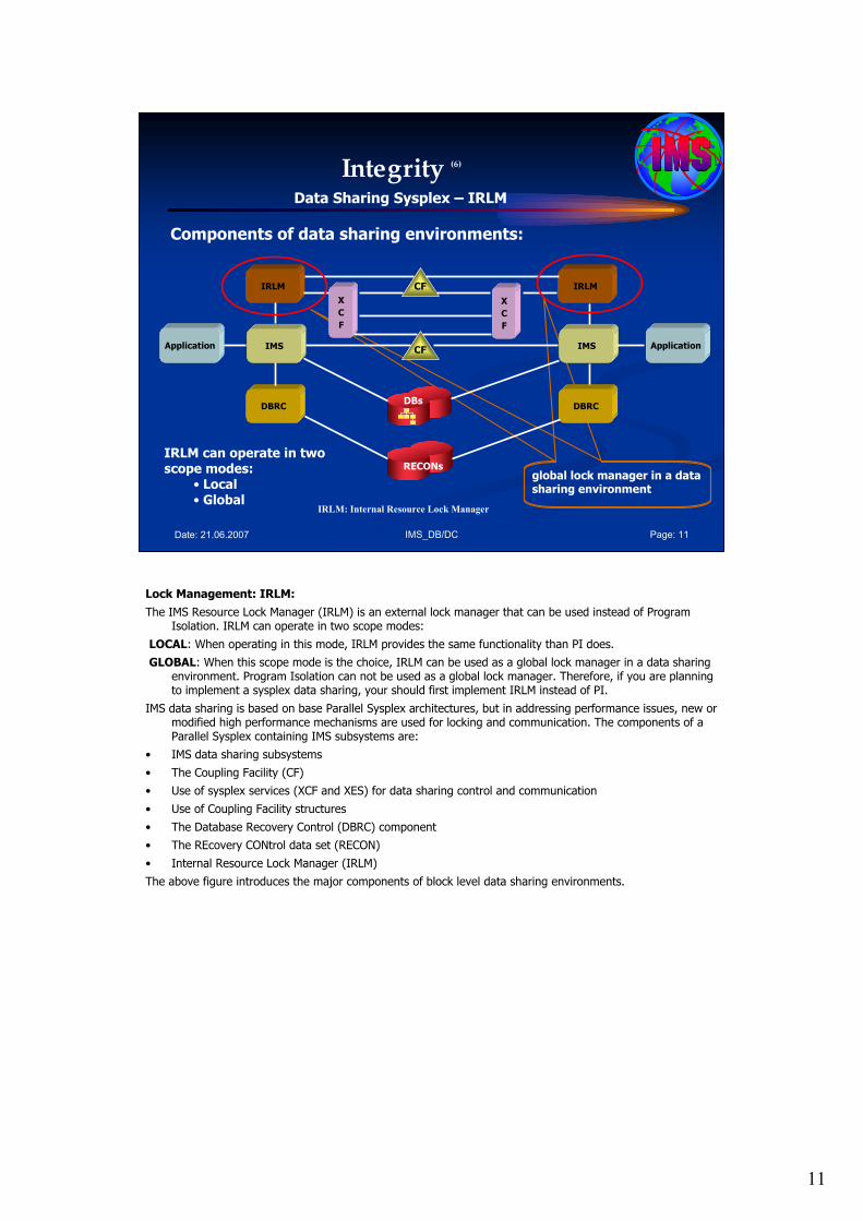
11
IMS_DB/DC Page: 11Date: 21.06.2007
Integrity (6)
Data Sharing Sysplex – IRLM
Components of data sharing environments:
IRLM
IMS
DBRC
Application
IRLM
IMS
DBRC
Application
X
C
F
X
C
F
CF
CF
DBs
RECONs
IRLM can operate in two scope modes:
• Local• Global
global lock manager in a data sharing environment
IRLM: Internal Resource Lock Manager
Lock Management: IRLM:
The IMS Resource Lock Manager (IRLM) is an external lock manager that can be used instead of Program Isolation. IRLM can operate in two scope modes:
LOCAL: When operating in this mode, IRLM provides the same functionality than PI does.
GLOBAL: When this scope mode is the choice, IRLM can be used as a global lock manager in a data sharing environment. Program Isolation can not be used as a global lock manager. Therefore, if you are planning to implement a sysplex data sharing, your should first implement IRLM instead of PI.
IMS data sharing is based on base Parallel Sysplex architectures, but in addressing performance issues, new or modified high performance mechanisms are used for locking and communication. The components of a Parallel Sysplex containing IMS subsystems are:
• IMS data sharing subsystems
• The Coupling Facility (CF)
• Use of sysplex services (XCF and XES) for data sharing control and communication
• Use of Coupling Facility structures
• The Database Recovery Control (DBRC) component
• The REcovery CONtrol data set (RECON)
• Internal Resource Lock Manager (IRLM)
The above figure introduces the major components of block level data sharing environments.
12
IMS_DB/DC Page: 12Date: 21.06.2007
Agenda Session 6: Data Sharing Issues
1. Integrity
2.Unit of Work
3. Commit Points / Sync Points
4. Locking
5. PROCOPTs
6. DL/I Calls
7. Deadlocks
8. Summary
2. Unit of Work
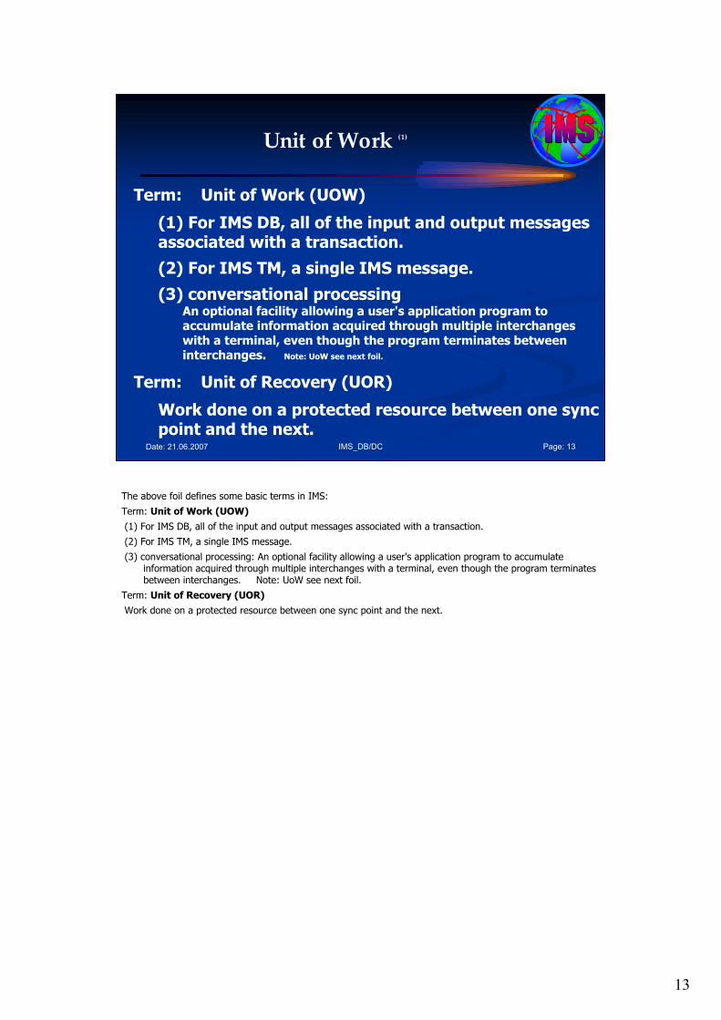
13
IMS_DB/DC Page: 13Date: 21.06.2007
Unit of Work (1)
Term: Unit of Work (UOW)
(1) For IMS DB, all of the input and output messages associated with a transaction.
(2) For IMS TM, a single IMS message.
(3) conversational processingAn optional facility allowing a user's application program to accumulate information acquired through multiple interchanges with a terminal, even though the program terminates between interchanges. Note: UoW see next foil.
Term: Unit of Recovery (UOR)
Work done on a protected resource between one sync point and the next.
The above foil defines some basic terms in IMS:
Term: Unit of Work (UOW)
(1) For IMS DB, all of the input and output messages associated with a transaction.
(2) For IMS TM, a single IMS message.
(3) conversational processing: An optional facility allowing a user's application program to accumulate information acquired through multiple interchanges with a terminal, even though the program terminates between interchanges. Note: UoW see next foil.
Term: Unit of Recovery (UOR)
Work done on a protected resource between one sync point and the next.
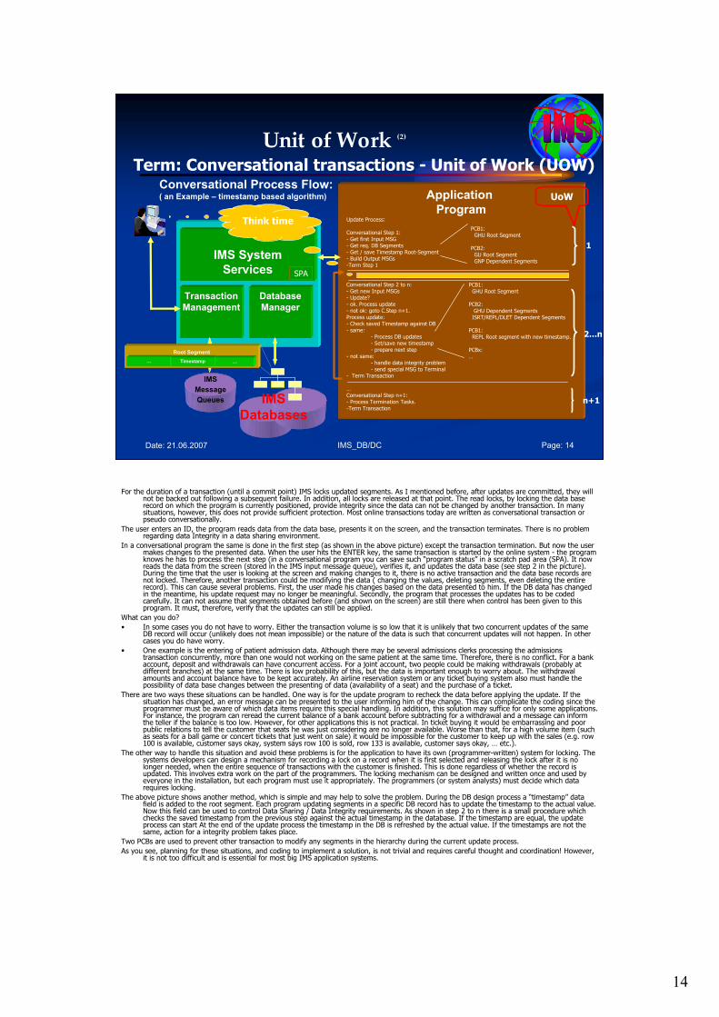
14
IMS_DB/DC Page: 14Date: 21.06.2007
Unit of Work (2)
Conversational Process Flow:( an Example – timestamp based algorithm)
IMS System
Services
Transaction
Management
Database
Manager
IMS
Message
Queues IMS
Databases
SPA
Application
ProgramUpdate Process:
Conversational Step 1:- Get first Input MSG- Get req. DB Segments- Get / save Timestamp Root-Segment- Build Output MSGs-Term Step 1
Conversational Step 2 to n:- Get new Input MSGs- Update?- ok. Process update - not ok: goto C.Step n+1.Process update:- Check saved Timestamp against DB - same:
- Process DB updates- Set/save new timestamp- prepare next step
- not same: - handle data integrity problem- send special MSG to Terminal
- Term Transaction
…Conversational Step n+1:- Process Termination Tasks. -Term Transaction
PCB1:GHU Root Segment
PCB2:GU Root SegmentGNP Dependent Segments
PCB1:GHU Root Segment
PCB2:GHU Dependent SegmentsISRT/REPL/DLET Dependent Segments
PCB1:REPL Root segment with new timestamp.
PCBx:…
Root Segment
… Timestamp …
Think time
Term: Conversational transactions - Unit of Work (UOW)
UoW
1
2…n
n+1
For the duration of a transaction (until a commit point) IMS locks updated segments. As I mentioned before, after updates are committed, they will not be backed out following a subsequent failure. In addition, all locks are released at that point. The read locks, by locking the data base record on which the program is currently positioned, provide integrity since the data can not be changed by another transaction. In many situations, however, this does not provide sufficient protection. Most online transactions today are written as conversational transaction or pseudo conversationally.
The user enters an ID, the program reads data from the data base, presents it on the screen, and the transaction terminates. There is no problem regarding data Integrity in a data sharing environment.
In a conversational program the same is done in the first step (as shown in the above picture) except the transaction termination. But now the user makes changes to the presented data. When the user hits the ENTER key, the same transaction is started by the online system - the program knows he has to process the next step (in a conversational program you can save such “program status” in a scratch pad area (SPA). It now reads the data from the screen (stored in the IMS input message queue), verifies it, and updates the data base (see step 2 in the picture). During the time that the user is looking at the screen and making changes to it, there is no active transaction and the data base records are not locked. Therefore, another transaction could be modifying the data ( changing the values, deleting segments, even deleting the entire record). This can cause several problems. First, the user made his changes based on the data presented to him. If the DB data has changed in the meantime, his update request may no longer be meaningful. Secondly, the program that processes the updates has to be coded carefully. It can not assume that segments obtained before (and shown on the screen) are still there when control has been given to this program. It must, therefore, verify that the updates can still be applied.
What can you do?
• In some cases you do not have to worry. Either the transaction volume is so low that it is unlikely that two concurrent updates of the same DB record will occur (unlikely does not mean impossible) or the nature of the data is such that concurrent updates will not happen. In other cases you do have worry.
• One example is the entering of patient admission data. Although there may be several admissions clerks processing the admissionstransaction concurrently, more than one would not working on the same patient at the same time. Therefore, there is no conflict. For a bank account, deposit and withdrawals can have concurrent access. For a joint account, two people could be making withdrawals (probably at different branches) at the same time. There is low probability of this, but the data is important enough to worry about. The withdrawal amounts and account balance have to be kept accurately. An airline reservation system or any ticket buying system also must handle the possibility of data base changes between the presenting of data (availability of a seat) and the purchase of a ticket.
There are two ways these situations can be handled. One way is for the update program to recheck the data before applying the update. If the situation has changed, an error message can be presented to the user informing him of the change. This can complicate the coding since the programmer must be aware of which data items require this special handling. In addition, this solution may suffice for only some applications. For instance, the program can reread the current balance of a bank account before subtracting for a withdrawal and a message can inform the teller if the balance is too low. However, for other applications this is not practical. In ticket buying it would be embarrassing and poor public relations to tell the customer that seats he was just considering are no longer available. Worse than that, for a high volume item (such as seats for a ball game or concert tickets that just went on sale) it would be impossible for the customer to keep up with the sales (e.g. row 100 is available, customer says okay, system says row 100 is sold, row 133 is available, customer says okay, … etc.).
The other way to handle this situation and avoid these problems is for the application to have its own (programmer-written) system for locking. The systems developers can design a mechanism for recording a lock on a record when it is first selected and releasing the lock after it is no longer needed, when the entire sequence of transactions with the customer is finished. This is done regardless of whether the record is updated. This involves extra work on the part of the programmers. The locking mechanism can be designed and written once and used by everyone in the installation, but each program must use it appropriately. The programmers (or system analysts) must decide which data requires locking.
The above picture shows another method, which is simple and may help to solve the problem. During the DB design process a “timestamp” data field is added to the root segment. Each program updating segments in a specific DB record has to update the timestamp to the actual value. Now this field can be used to control Data Sharing / Data Integrity requirements. As shown in step 2 to n there is a small procedure which checks the saved timestamp from the previous step against the actual timestamp in the database. If the timestamp are equal, the update process can start At the end of the update process the timestamp in the DB is refreshed by the actual value. If the timestamps are not the same, action for a integrity problem takes place.
Two PCBs are used to prevent other transaction to modify any segments in the hierarchy during the current update process.
As you see, planning for these situations, and coding to implement a solution, is not trivial and requires careful thought and coordination! However, it is not too difficult and is essential for most big IMS application systems.
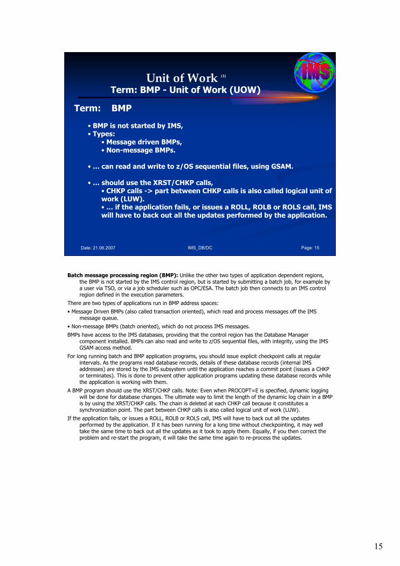
15
IMS_DB/DC Page: 15Date: 21.06.2007
Unit of Work (3)
Term: BMP - Unit of Work (UOW)
Term: BMP
• BMP is not started by IMS,• Types:
• Message driven BMPs,• Non-message BMPs.
•… can read and write to z/OS sequential files, using GSAM.
•… should use the XRST/CHKP calls,• CHKP calls -> part between CHKP calls is also called logical unit of work (LUW).•… if the application fails, or issues a ROLL, ROLB or ROLS call, IMS will have to back out all the updates performed by the application.
Batch message processing region (BMP): Unlike the other two types of application dependent regions, the BMP is not started by the IMS control region, but is started by submitting a batch job, for example by a user via TSO, or via a job scheduler such as OPC/ESA. The batch job then connects to an IMS control region defined in the execution parameters.
There are two types of applications run in BMP address spaces:
• Message Driven BMPs (also called transaction oriented), which read and process messages off the IMS message queue.
• Non-message BMPs (batch oriented), which do not process IMS messages.
BMPs have access to the IMS databases, providing that the control region has the Database Manager component installed. BMPs can also read and write to z/OS sequential files, with integrity, using the IMS GSAM access method.
For long running batch and BMP application programs, you should issue explicit checkpoint calls at regular intervals. As the programs read database records, details of these database records (internal IMS addresses) are stored by the IMS subsystem until the application reaches a commit point (issues a CHKP or terminates). This is done to prevent other application programs updating these database records while the application is working with them.
A BMP program should use the XRST/CHKP calls. Note: Even when PROCOPT=E is specified, dynamic logging will be done for database changes. The ultimate way to limit the length of the dynamic log chain in a BMP is by using the XRST/CHKP calls. The chain is deleted at each CHKP call because it constitutes a synchronization point. The part between CHKP calls is also called logical unit of work (LUW).
If the application fails, or issues a ROLL, ROLB or ROLS call, IMS will have to back out all the updates performed by the application. If it has been running for a long time without checkpointing, it may well take the same time to back out all the updates as it took to apply them. Equally, if you then correct the problem and re-start the program, it will take the same time again to re-process the updates.
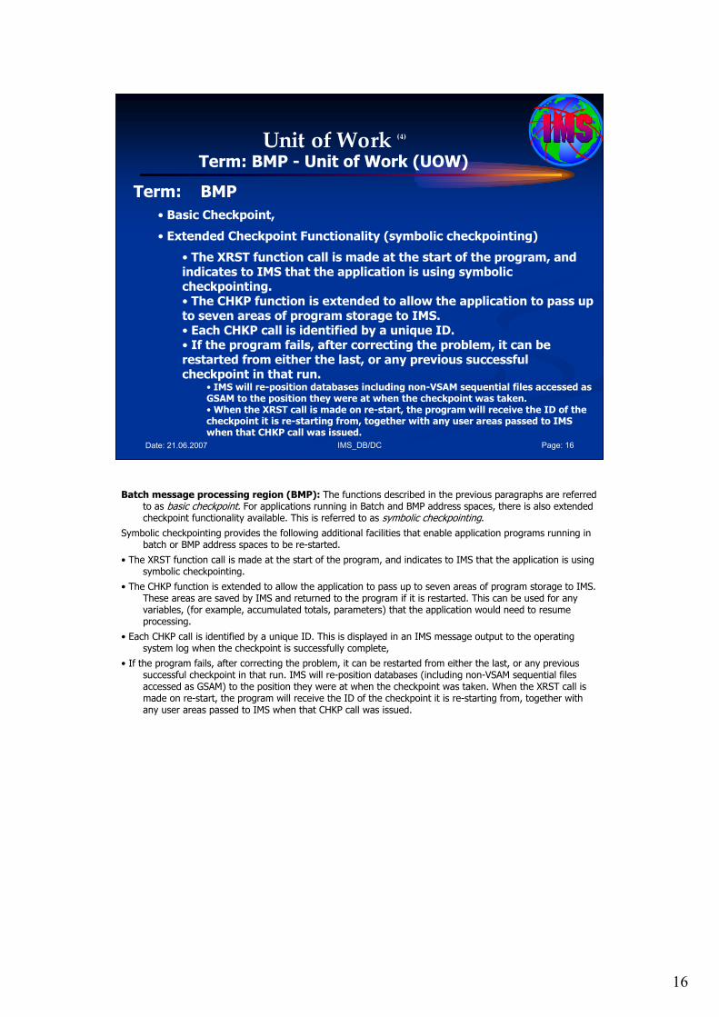
16
IMS_DB/DC Page: 16Date: 21.06.2007
Unit of Work (4)
Term: BMP - Unit of Work (UOW)
Term: BMP
• Basic Checkpoint,
• Extended Checkpoint Functionality (symbolic checkpointing)
• The XRST function call is made at the start of the program, andindicates to IMS that the application is using symbolic checkpointing.• The CHKP function is extended to allow the application to pass up to seven areas of program storage to IMS.• Each CHKP call is identified by a unique ID.• If the program fails, after correcting the problem, it can be restarted from either the last, or any previous successful checkpoint in that run.
• IMS will re-position databases including non-VSAM sequential files accessed as GSAM to the position they were at when the checkpoint was taken.•When the XRST call is made on re-start, the program will receive the ID of the checkpoint it is re-starting from, together with any user areas passed to IMS when that CHKP call was issued.
Batch message processing region (BMP): The functions described in the previous paragraphs are referred to as basic checkpoint. For applications running in Batch and BMP address spaces, there is also extended checkpoint functionality available. This is referred to as symbolic checkpointing.
Symbolic checkpointing provides the following additional facilities that enable application programs running in batch or BMP address spaces to be re-started.
• The XRST function call is made at the start of the program, and indicates to IMS that the application is using symbolic checkpointing.
• The CHKP function is extended to allow the application to pass up to seven areas of program storage to IMS. These areas are saved by IMS and returned to the program if it is restarted. This can be used for any variables, (for example, accumulated totals, parameters) that the application would need to resume processing.
• Each CHKP call is identified by a unique ID. This is displayed in an IMS message output to the operating system log when the checkpoint is successfully complete,
• If the program fails, after correcting the problem, it can be restarted from either the last, or any previous successful checkpoint in that run. IMS will re-position databases (including non-VSAM sequential files accessed as GSAM) to the position they were at when the checkpoint was taken. When the XRST call is made on re-start, the program will receive the ID of the checkpoint it is re-starting from, together with any user areas passed to IMS when that CHKP call was issued.
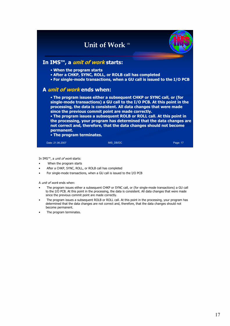
17
IMS_DB/DC Page: 17Date: 21.06.2007
Unit of Work (5)
In IMS™, a unit of work starts:
•When the program starts• After a CHKP, SYNC, ROLL, or ROLB call has completed• For single-mode transactions, when a GU call is issued to the I/O PCB
A unit of work ends when:
• The program issues either a subsequent CHKP or SYNC call, or (for single-mode transactions) a GU call to the I/O PCB. At this point in the processing, the data is consistent. All data changes that were made since the previous commit point are made correctly.• The program issues a subsequent ROLB or ROLL call. At this point in the processing, your program has determined that the data changes are not correct and, therefore, that the data changes should not become permanent.• The program terminates.
In IMS™, a unit of work starts:
• When the program starts
• After a CHKP, SYNC, ROLL, or ROLB call has completed
• For single-mode transactions, when a GU call is issued to the I/O PCB
A unit of work ends when:
• The program issues either a subsequent CHKP or SYNC call, or (for single-mode transactions) a GU call to the I/O PCB. At this point in the processing, the data is consistent. All data changes that were made since the previous commit point are made correctly.
• The program issues a subsequent ROLB or ROLL call. At this point in the processing, your program has determined that the data changes are not correct and, therefore, that the data changes should not become permanent.
• The program terminates.
18
IMS_DB/DC Page: 18Date: 21.06.2007
Agenda Session 6: Data Sharing Issues
1. Integrity
2. Unit of Work
3. Commit Points / Sync Points
4. Locking
5. PROCOPTs
6. DL/I Calls
7. Deadlocks
8. Summary
3. Commit Points / Sync Points
19
IMS_DB/DC Page: 19Date: 21.06.2007
Commit Points (1)
• A commit point is the place in the program’s processing at which it completes a unit of work,
•When a unit of work is completed, IMS commit the changes that your program made to the database.
• Those changes are now permanent and the changed data is now available to other application programs.
Commit Points: When an online program accesses the database, it is not necessarily the only program doing so. IMS make it possible for more than one application program to access the data concurrently without endangering the integrity of the data. To access data concurrently while protecting data integrity, IMS prevent other application programs from accessing segments that your program deletes, replaces, or inserts, until your program reaches a commit point. A commit point is the place in the program’s processing at which it completes a unit of work. When a unit of work is completed, IMS commit the changes that your program made to the database. Those changes are now permanent and the changed data is now available to other application programs.

20
IMS_DB/DC Page: 20Date: 21.06.2007
Commit Points (2)
•What Happens at a Commit Point:
• A commit point indicates to IMS that a program has finished a unit of work:
• IMS releases segments it has locked for the program since the last commit point. Those segments are then available to other application programs.• IMS make the program’s changes to the database permanent.• The current position in all databases except GSAM is reset to the start of the database.
• If the program terminates abnormally before reaching the commitpoint:
• IMS back out all of the changes the program has made to the database since the last commit point. • IMS discards any output messages that the program has produced since the last commit point.
What Happens at a Commit Point: When an application program finishes processing one distinct unit of
work, IMS consider that processing to be valid, even if the program later encounters problems. For example, an application program that is retrieving, processing, and responding to a message from a terminal constitutes a unit of work. If the program encounters problems while processing the next input message, the processing it has done on the first input message is not affected. These input messages are separate pieces of processing. A commit point indicates to IMS that a program has finished a unit of work, and that the processing it has done is accurate. At that time:
• IMS releases segments it has locked for the program since the last commit point. Those segments are then available to other application programs.
• IMS and DB2 UDB for z/OS make the program’s changes to the database permanent.
• The current position in all databases except GSAM is reset to the start of the database.
If the program terminates abnormally before reaching the commit point:
• IMS back out all of the changes the program has made to the database since the last commit point. (This does not apply to batch programs that write their log to tape.)
• IMS discards any output messages that the program has produced since the last commit point. Until the program reaches a commit point, IMS holds the program’s output messages so that, if the program terminates abnormally, users at terminals and other application programs do not receive inaccurate information from the abnormally terminating application program.
If the program is processing an input message and terminates abnormally, the input message is not discarded if both of the following conditions exist:
1. You are not using the Non-Discardable Messages (NDM) exit routine.
2. 2. IMS terminates the program with one of the following abend codes: U0777, U2478, U2479, U3303. The input message is saved and processed later. Exception: The input message is discarded if it is not terminated by one of the abend codes previously referenced. When the program is restarted, IMS gives the program the next message. If the program is processing an input message when it terminates abnormally, and you use the NDM exit routine, the input message might be discarded from the system regardless of the abend. Whether the input message is discarded from the system depends on how you have written the NDM exit routine.
• IMS notifies the MTO that the program terminated abnormally.
• IMS and DB2 UDB for z/OS release any locks that the program has held on data it has updated since the last commit point. This makes the data available to other application programs and users.
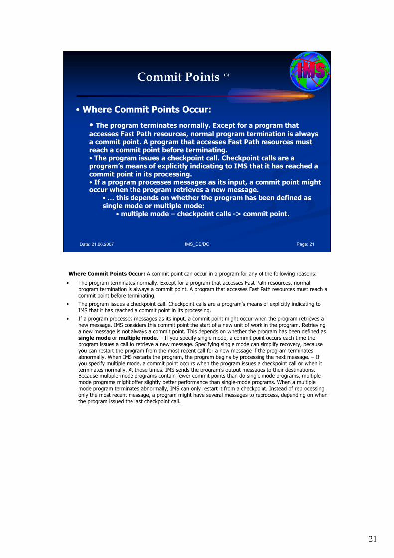
21
IMS_DB/DC Page: 21Date: 21.06.2007
Commit Points (3)
•Where Commit Points Occur:
• The program terminates normally. Except for a program that accesses Fast Path resources, normal program termination is always a commit point. A program that accesses Fast Path resources mustreach a commit point before terminating.• The program issues a checkpoint call. Checkpoint calls are a program’s means of explicitly indicating to IMS that it has reached a commit point in its processing.• If a program processes messages as its input, a commit point might occur when the program retrieves a new message.
•… this depends on whether the program has been defined as single mode or multiple mode:
• multiple mode – checkpoint calls -> commit point.
Where Commit Points Occur: A commit point can occur in a program for any of the following reasons:
• The program terminates normally. Except for a program that accesses Fast Path resources, normal program termination is always a commit point. A program that accesses Fast Path resources must reach a commit point before terminating.
• The program issues a checkpoint call. Checkpoint calls are a program’s means of explicitly indicating to IMS that it has reached a commit point in its processing.
• If a program processes messages as its input, a commit point might occur when the program retrieves a new message. IMS considers this commit point the start of a new unit of work in the program. Retrieving a new message is not always a commit point. This depends on whether the program has been defined as single mode or multiple mode. – If you specify single mode, a commit point occurs each time theprogram issues a call to retrieve a new message. Specifying single mode can simplify recovery, because you can restart the program from the most recent call for a new message if the program terminates abnormally. When IMS restarts the program, the program begins by processing the next message. – If you specify multiple mode, a commit point occurs when the program issues a checkpoint call or when it terminates normally. At those times, IMS sends the program’s output messages to their destinations. Because multiple-mode programs contain fewer commit points than do single mode programs, multiple mode programs might offer slightly better performance than single-mode programs. When a multiple mode program terminates abnormally, IMS can only restart it from a checkpoint. Instead of reprocessing only the most recent message, a program might have several messages to reprocess, depending on when the program issued the last checkpoint call.

22
IMS_DB/DC Page: 22Date: 21.06.2007
Sync Point/SYNC Call (1)
• SYNC Call (Fast Path):
• Ensure that BMPs accessing DEDBs issue SYNC calls at frequent intervals. (BMPs could be designed to issue many calls between sync points and so gain exclusive control over a significant number of CIs.)
• BMPs that do physical-sequential processing through a DEDB should issue a SYNC call when crossing a CI boundary (provided it is possible to calculate this point). This ensures that the application program never holds more than a single CI.
SYNC Call (Fast Path):
Ensure that BMPs accessing DEDBs issue SYNC calls at frequent intervals. (BMPs could be designed to issue many calls between sync points and so gain exclusive control over a significant number of CIs.)
BMPs that do physical-sequential processing through a DEDB should issue a SYNC call when crossing a CI boundary (provided it is possible to calculate this point). This ensures that the application program never holds more than a single CI.

23
IMS_DB/DC Page: 23Date: 21.06.2007
Agenda Session 6: Data Sharing Issues
1. Integrity
2. Unit of Work
3. Commit Points / Sync Points
4. Locking
5. PROCOPTs
6. DL/I Calls
7. Deadlocks
8. Summary
4. Locking
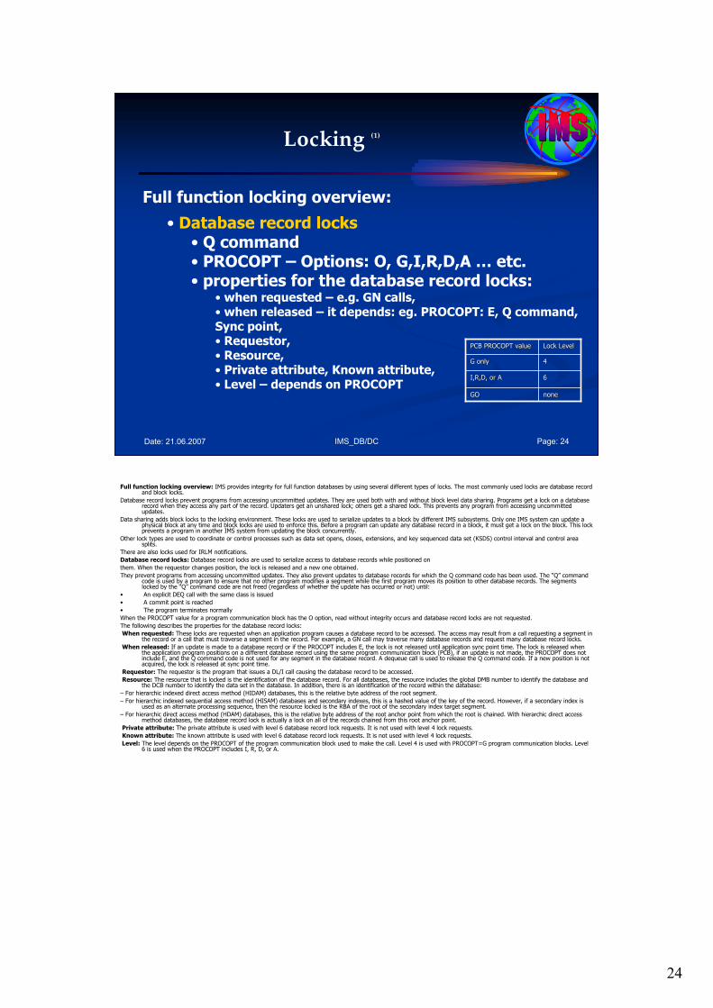
24
IMS_DB/DC Page: 24Date: 21.06.2007
Locking (1)
Full function locking overview:
• Database record locks• Q command• PROCOPT – Options: O, G,I,R,D,A … etc.• properties for the database record locks:
• when requested – e.g. GN calls,• when released – it depends: eg. PROCOPT: E, Q command, Sync point,• Requestor,• Resource,• Private attribute, Known attribute,• Level – depends on PROCOPT
nonenoneGOGO
66I,R,D, or AI,R,D, or A
44G onlyG only
Lock LevelLock LevelPCB PROCOPT valuePCB PROCOPT value
Full function locking overview: IMS provides integrity for full function databases by using several different types of locks. The most commonly used locks are database record and block locks.
Database record locks prevent programs from accessing uncommitted updates. They are used both with and without block level data sharing. Programs get a lock on a database record when they access any part of the record. Updaters get an unshared lock; others get a shared lock. This prevents any program from accessing uncommitted updates.
Data sharing adds block locks to the locking environment. These locks are used to serialize updates to a block by different IMS subsystems. Only one IMS system can update a physical block at any time and block locks are used to enforce this. Before a program can update any database record in a block, it must get a lock on the block. This lock prevents a program in another IMS system from updating the block concurrently.
Other lock types are used to coordinate or control processes such as data set opens, closes, extensions, and key sequenced data set (KSDS) control interval and control area splits.
There are also locks used for IRLM notifications.
Database record locks: Database record locks are used to serialize access to database records while positioned on
them. When the requestor changes position, the lock is released and a new one obtained.
They prevent programs from accessing uncommitted updates. They also prevent updates to database records for which the Q command code has been used. The “Q” command code is used by a program to ensure that no other program modifies a segment while the first program moves its position to other database records. The segments locked by the “Q” command code are not freed (regardless of whether the update has occurred or not) until:
• An explicit DEQ call with the same class is issued
• A commit point is reached
• The program terminates normally
When the PROCOPT value for a program communication block has the O option, read without integrity occurs and database record locks are not requested.
The following describes the properties for the database record locks:
When requested: These locks are requested when an application program causes a database record to be accessed. The access may result from a call requesting a segment in the record or a call that must traverse a segment in the record. For example, a GN call may traverse many database records and request many database record locks.
When released: If an update is made to a database record or if the PROCOPT includes E, the lock is not released until application sync point time. The lock is released when the application program positions on a different database record using the same program communication block (PCB), if an update is not made, the PROCOPT does not include E, and the Q command code is not used for any segment in the database record. A dequeue call is used to release the Q command code. If a new position is not acquired, the lock is released at sync point time.
Requestor: The requestor is the program that issues a DL/I call causing the database record to be accessed.
Resource: The resource that is locked is the identification of the database record. For all databases, the resource includes the global DMB number to identify the database and the DCB number to identify the data set in the database. In addition, there is an identification of the record within the database:
– For hierarchic indexed direct access method (HIDAM) databases, this is the relative byte address of the root segment.
– For hierarchic indexed sequential access method (HISAM) databases and secondary indexes, this is a hashed value of the key of the record. However, if a secondary index is used as an alternate processing sequence, then the resource locked is the RBA of the root of the secondary index target segment.
– For hierarchic direct access method (HDAM) databases, this is the relative byte address of the root anchor point from which the root is chained. With hierarchic direct access method databases, the database record lock is actually a lock on all of the records chained from this root anchor point.
Private attribute: The private attribute is used with level 6 database record lock requests. It is not used with level 4 lock requests.
Known attribute: The known attribute is used with level 6 database record lock requests. It is not used with level 4 lock requests.
Level: The level depends on the PROCOPT of the program communication block used to make the call. Level 4 is used with PROCOPT=G program communication blocks. Level 6 is used when the PROCOPT includes I, R, D, or A.
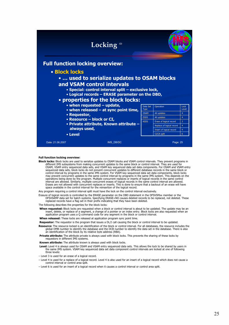
25
IMS_DB/DC Page: 25Date: 21.06.2007
Locking (2)
Full function locking overview:
• Block locks•… used to serialize updates to OSAM blocks and VSAM control intervals
• Special: control interval split – exclusive lock,• Logical records – ERASE parameter on the DBD,
• properties for the block locks:• when requested – update,• when released – at sync point time,• Requestor,• Resource – block or CI,• Private attribute, Known attribute –always used,
• Level 66CI/CA splitCI/CA split
44Insert of logical recordInsert of logical record
44Replace of logical recordReplace of logical record
33Erase of logical recordErase of logical recordKSDSKSDS
44All updatesAll updatesESDSESDS
44All updatesAll updatesOSAMOSAM
Lock Lock
LevelLevelOperationOperationData Set Data Set
TypeType
Full function locking overview:
Block locks: Block locks are used to serialize updates to OSAM blocks and VSAM control intervals. They prevent programs in different IMS subsystems from making concurrent updates to the same block or control interval. They are used for OSAM, VSAM entry sequenced data sets, and VSAM key sequenced data set data components. For OSAM and VSAM entry sequenced data sets, block locks do not prevent concurrent updates to different database records in the same block or control interval by programs in the same IMS system. For VSAM key sequenced data set data components, block locks may prevent concurrent updates to the same control interval by programs in the same IMS system. This depends on the operations being done by the program. Multiple concurrent replaces or inserts of logical records in the same control interval are allowed. Similarly, multiple concurrent erases of logical records in the same control interval are allowed. Erases are not allowed with concurrent replaces or inserts. This is done to ensure that a backout of an erase will have space available in the control interval for the reinsertion of the logical record.
Any program requiring a control interval split must have the lock on the control interval exclusively.
Erasure of logical records is controlled by the ERASE parameter on the DBD statement in the DFSVSMxx member or the DFSVSAMP data set for batch systems. Specifying ERASE=NO causes deleted records to be replaced, not deleted. These replaced records have a flag set in their prefix indicating that they have been deleted.
The following describes the properties for the block locks:
When requested: Block locks are requested when a block or control interval is about to be updated. The update may be an insert, delete, or replace of a segment, a change of a pointer or an index entry. Block locks are also requested when an application program uses a Q command code for any segment in the block or control interval.
When released: These locks are released at application program sync point time.
Requestor: The requestor is the program that issues a DL/I call causing the block or control interval to be updated.
Resource: The resource locked is an identification of the block or control interval. For all databases, the resource includes the global DMB number to identify the database and the DCB number to identify the data set in the database. There is also an identification of the block by its relative byte address (RBA).
Private attribute: The attribute private is always used with block locks. This prevents the sharing of these locks by requestors in different IMS systems.
Known attribute: The attribute known is always used with block locks.
Level: Level 4 is always used for OSAM and VSAM entry sequenced data sets. This allows the lock to be shared by users in the same IMS system. VSAM key sequenced data set data component control intervals are locked at one of following three levels:
– Level 3 is used for an erase of a logical record.
– Level 4 is used for a replace of a logical record. Level 4 is also used for an insert of a logical record which does not cause a control interval or control area split.
– Level 6 is used for an insert of a logical record when it causes a control interval or control area split.
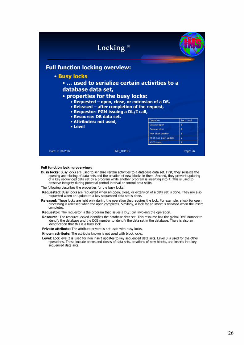
26
IMS_DB/DC Page: 26Date: 21.06.2007
Locking (3)
Full function locking overview:
• Busy locks•… used to serialize certain activities to a database data set,• properties for the busy locks:
• Requested – open, close, or extension of a DS,• Released – after completion of the request,• Requestor: PGM issuing a DL/I call,• Resource: DB data set,• Attributes: not used,• Level
88KSDS insertKSDS insert
22KSDS non insert updateKSDS non insert update
88New block creationNew block creation
88Data set closeData set close
88Data set openData set open
Lock LevelLock LevelOperationOperation
Full function locking overview:
Busy locks: Busy locks are used to serialize certain activities to a database data set. First, they serialize the opening and closing of data sets and the creation of new blocks in them. Second, they prevent updating of a key sequenced data set by a program while another program is inserting into it. This is used to preserve integrity during potential control interval or control area splits.
The following describes the properties for the busy locks:
Requested: Busy locks are requested when an open, close, or extension of a data set is done. They are also requested when an update to a key sequenced data set is done.
Released: These locks are held only during the operation that requires the lock. For example, a lock for open processing is released when the open completes. Similarly, a lock for an insert is released when the insert completes.
Requestor: The requestor is the program that issues a DL/I call invoking the operation.
Resource: The resource locked identifies the database data set. This resource has the global DMB number to identify the database and the DCB number to identify the data set in the database. There is also an identification that this is a busy lock.
Private attribute: The attribute private is not used with busy locks.
Known attribute: The attribute known is not used with block locks.
Level: Lock level 2 is used for non insert updates to key sequenced data sets. Level 8 is used for the other operations. These include opens and closes of data sets, creations of new blocks, and inserts into key sequenced data sets.
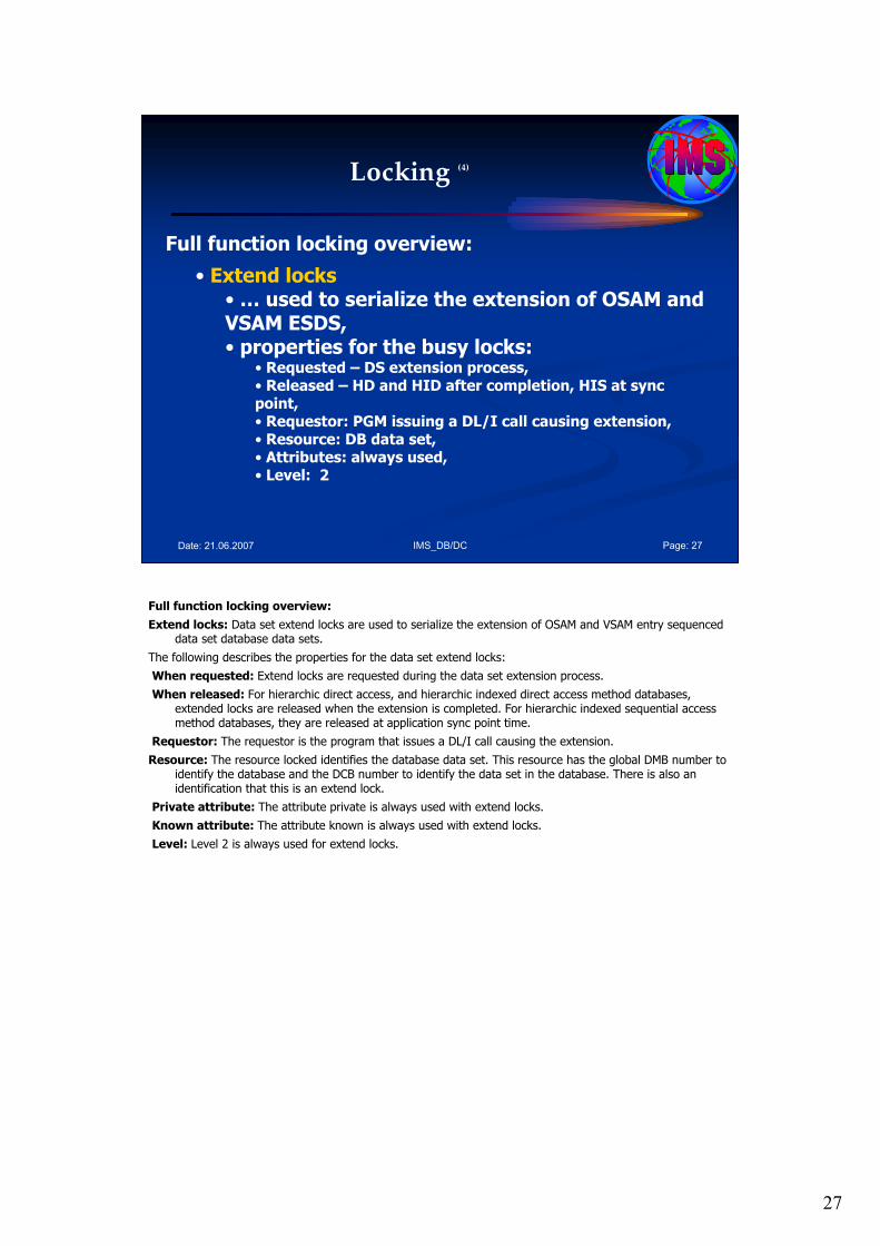
27
IMS_DB/DC Page: 27Date: 21.06.2007
Locking (4)
Full function locking overview:
• Extend locks•… used to serialize the extension of OSAM and VSAM ESDS,• properties for the busy locks:
• Requested – DS extension process,• Released – HD and HID after completion, HIS at sync point,• Requestor: PGM issuing a DL/I call causing extension, • Resource: DB data set,• Attributes: always used,• Level: 2
Full function locking overview:
Extend locks: Data set extend locks are used to serialize the extension of OSAM and VSAM entry sequenced data set database data sets.
The following describes the properties for the data set extend locks:
When requested: Extend locks are requested during the data set extension process.
When released: For hierarchic direct access, and hierarchic indexed direct access method databases, extended locks are released when the extension is completed. For hierarchic indexed sequential access method databases, they are released at application sync point time.
Requestor: The requestor is the program that issues a DL/I call causing the extension.
Resource: The resource locked identifies the database data set. This resource has the global DMB number to identify the database and the DCB number to identify the data set in the database. There is also an identification that this is an extend lock.
Private attribute: The attribute private is always used with extend locks.
Known attribute: The attribute known is always used with extend locks.
Level: Level 2 is always used for extend locks.
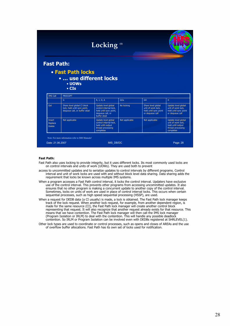
28
IMS_DB/DC Page: 28Date: 21.06.2007
Locking (5)
Fast Path:
• Fast Path locks•… use different locks
• UOWs• CIs
Note: For more information refer to IMS Manuals!
HHGHGHGOxGOxR, I, D, AR, I, D, AGG
Update level global Update level global
unit of work lock, unit of work lock,
held until output held until output
thread processing thread processing
completescompletes
Not applicableNot applicableNot applicableNot applicableUpdate level global Update level global
control internal lock, control internal lock,
held until output held until output
thread processing thread processing
completes completes
Not applicableNot applicableInsertInsert
ReplaceReplace
DeleteDelete
Update level global Update level global
unit of work lock, unit of work lock,
held until sync point held until sync point
or dequeue call or dequeue call
Share level global Share level global
unit of work lock, unit of work lock,
held until sync point held until sync point
or dequeue callor dequeue call
No lockingNo lockingUpdate level global Update level global
control internal lock, control internal lock,
held until sync point, held until sync point,
dequeue call, or dequeue call, or
buffer stealbuffer steal
Share level global CI block Share level global CI block
lock, held until sync point, lock, held until sync point,
dequeue call, or buffer stealdequeue call, or buffer steal
GetGet
PROCOPTPROCOPTIMS CallIMS Call
Fast Path:
Fast Path also uses locking to provide integrity, but it uses different locks. Its most commonly used locks are on control intervals and units of work (UOWs). They are used both to prevent
access to uncommitted updates and to serialize updates to control intervals by different programs. Control interval and unit of work locks are used with and without block level data sharing. Data sharing adds the requirement that locks be known across multiple IMS systems.
When a program accesses a Fast Path control interval, it locks the control interval. Updaters have exclusive use of the control interval. This prevents other programs from accessing uncommitted updates. It also ensures that no other program is making a concurrent update to another copy of the control interval. Sometimes, locks on units of work are used in place of control interval locks. This occurs when certain sequential processes, such as high speed sequential processing (HSSP), are used.
When a request for DEDB data (a CI usually) is made, a lock is obtained. The Fast Path lock manager keeps track of the lock request. When another lock request, for example, from another dependent region, is made for the same resource (CI), the Fast Path lock manager will create another control block representing that request. It will also recognize that another request already exists for that resource. This means that we have contention. The Fast Path lock manager will then call the IMS lock manager (Program Isolation or IRLM) to deal with the contention. This will handle any possible deadlock contention. So IRLM or Program Isolation can be involved even with DEDBs registered at SHRLEVEL(1).
Other lock types are used to coordinate or control processes, such as opens and closes of AREAs and the use of overflow buffer allocations. Fast Path has its own set of locks used for notification.
29
IMS_DB/DC Page: 29Date: 21.06.2007
Locking (6)
Specific use of locks and their effect in data sharing:
• Locks obtained when:
• searching for free space,• maintaining DB pointers,• communicating global notifications,• serializing CA/CI splits,• extending databases.
Note: For more information refer to IMS Manuals!
Specific use of locks and their effect in data sharing: Additional locks are obtained by IMS to maintain recoverability and integrity. Locks are obtained when searching for free space, maintaining database pointers, communicating global notifications between subsystems, serializing control interval/control area splits, and extending databases.
30
IMS_DB/DC Page: 30Date: 21.06.2007
Locking (7)
Resource Locking Considerations with Block Level Sharing:
• non-sysplex environment, local locks: • Immediately • synchronously
• sysplex environment, global locks: • Locally by the IRLM • Synchronously on the XES CALL • Asynchronously on the XES CALL
Note: For more information refer to IMS Manuals!
Resource Locking Considerations with Block Level Sharing: Resource locking can occur either locally in a non-sysplex environment or globally in a sysplex environment. In a non-sysplex environment, local locks can be granted in one of three ways:
• Immediately because of one of the following reasons: IMS was able to get the required IRLM locks, and there is no other interest on this resource. The request is compatible with other holders or waiters.
• Asynchronously because the request could not get the required IRLM latches and was suspended. (This can also occur in a sysplex environment.) The lock is granted when latches become available and one of three conditions exist: No other holders exist. The request is compatible with other holders or waiters. The request is not compatible with the holders or waiters and was granted after their interest was released. (This could also occur in a sysplex environment.)
In a sysplex environment, global locks can be granted in one of three ways:
• Locally by the IRLM because of one of the following reasons: There is no other interest for this resource. This IRLM has the only interest, this request is compatible with the holders or waiters on this system, and XES already knows about the resource.
• Synchronously on the XES CALL because of one of the following reasons: XES shows no other interest for this resource. XES shows only SHARE interest for the hash class.
• Asynchronously on the XES CALL because of one of three conditions: Either XES shows EXCLUSIVE interest on the hash class by an IRLM, but the resource names do not match (FALSE CONTENTION by RMF™). Or XES shows EXCLUSIVE interest on the hash class by an IRLM and the resource names match, but the IRLM CONTENTION EXIT grants it anyway because the STATES are compatible (IRLM FALSE CONTENTION). Or the request is incompatible with the other HOLDERs and is granted by the CONTENTION Exit after their interest is released (IRLM REAL CONTENTION).
31
IMS_DB/DC Page: 31Date: 21.06.2007
Locking (8)
Data Sharing Impact on Locking:
•When you use block-level data sharing, the IRLM must obtain the concurrence of the sharing system before granting global locks.
• Root locks are global locks, and dependent segment locks are not.
•When you use block-level data sharing, locks prevent the sharing systems from concurrently updating the same buffer. The buffer is locked before making the update, and the lock is held until after the buffer is written during commit processing.
• No buffer locks are obtained when a buffer is read.
Note: For more information refer to IMS Manuals!
Data Sharing Impact on Locking: When you use block-level data sharing, the IRLM must obtain the concurrence of the sharing system before granting global locks. Root locks are global locks, and dependent segment locks are not. When you use block-level data sharing, locks prevent the sharing systems from concurrently updating the same buffer. The buffer is locked before making the update, and the lock is held until after the buffer is written during commit processing. No buffer locks are obtained when a buffer is read.
If a Q command code is issued on any segment, the buffer is locked. This prevents the sharing system from updating the buffer until the Q command code lock is released.
32
IMS_DB/DC Page: 32Date: 21.06.2007
Locking (9)
Locking for Secondary Indexes:
•When a secondary index is inserted, deleted or replaced, it is locked with a root segment lock.
•When the secondary index is used to access the target of the secondary index, depending on what the index points to, it might be necessary to lock the secondary index.
Note: For more information refer to IMS Manuals!
Locking for Secondary Indexes: When a secondary index is inserted, deleted or replaced, it is locked with a root segment lock. When the secondary index is used to access the target of the secondary index, depending on what the index points to, it might be necessary to lock the secondary index.
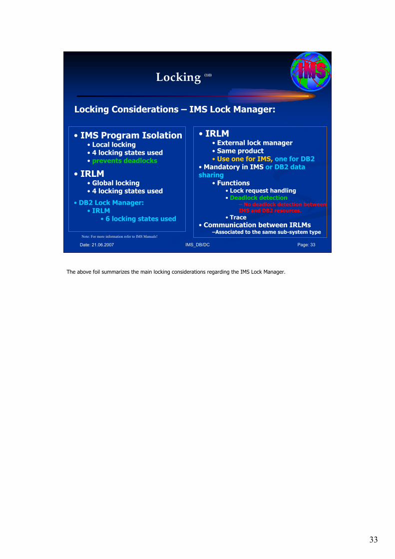
33
IMS_DB/DC Page: 33Date: 21.06.2007
Locking (10)
Locking Considerations – IMS Lock Manager:
Note: For more information refer to IMS Manuals!
• IMS Program Isolation• Local locking• 4 locking states used• prevents deadlocks
• IRLM• Global locking• 4 locking states used
• DB2 Lock Manager:• IRLM
• 6 locking states used
• IRLM• External lock manager• Same product• Use one for IMS, one for DB2
• Mandatory in IMS or DB2 data sharing
• Functions• Lock request handling• Deadlock detection
– No deadlock detection between IMS and DB2 resources.
• Trace
• Communication between IRLMs–Associated to the same sub-system type
The above foil summarizes the main locking considerations regarding the IMS Lock Manager.
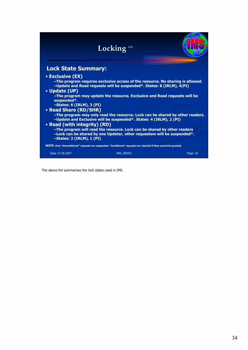
34
IMS_DB/DC Page: 34Date: 21.06.2007
Locking (11)
Lock State Summary:
• Exclusive (EX) –The program requires exclusive access of the resource. No sharing is allowed.–Update and Read requests will be suspended*. States: 8 (IRLM), 4(PI)
• Update (UP)–The program may update the resource. Exclusive and Read requests will be suspended*.–States: 6 (IRLM), 3 (PI)
• Read Share (RD/SHR)–The program may only read the resource. Lock can be shared by other readers.–Update and Exclusive will be suspended*. States: 4 (IRLM), 2 (PI)
• Read (with integrity) (RD) –The program will read the resource. Lock can be shared by other readers–Lock can be shared by one Updater, other requestors will be suspended*.–States: 2 (IRLM), 1 (PI)
NOTE: Only “Unconditional” requests are suspended. “Conditional” requests are rejected if they cannot be granted.
The above foil summarizes the lock states used in IMS.

35
IMS_DB/DC Page: 35Date: 21.06.2007
Agenda Session 6: Data Sharing Issues
1. Integrity
2. Unit of Work
3. Commit Points / Sync Points
4. Locking
5. PROCOPTs
6. DL/I Calls
7. Deadlocks
8. Summary
5. PROCOPTs
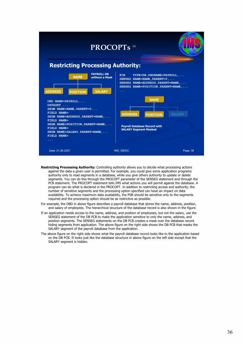
36
IMS_DB/DC Page: 36Date: 21.06.2007
PROCOPTs (1)
Restricting Processing Authority:
DBD NAME=PAYROLL,...
DATASET ...
SEGM NAME=NAME,PARENT=0...
FIELD NAME=
SEGM NAME=ADDRESS,PARENT=NAME,...
FIELD NAME=
SEGM NAME=POSITION,PARENT=NAME,...
FIELD NAME=
SEGM NAME=SALARY,PARENT=NAME,...
FIELD NAME=
...
POSITION
NAME
ADDRESS SALARY
PAYROLL DB without a Mask
PCB TYPE=DB,DBDNAME=PAYROLL,...
SENSEG NAME=NAME,PARENT=0,...
SENSEG NAME=ADDRESS,PARENT=NAME,...
SENSEG NAME=POSITION,PARENT=NAME,...
...
POSITION
NAME
ADDRESS SALARY
Payroll Database Record with SALARY Segment Masked
Restricting Processing Authority: Controlling authority allows you to decide what processing actions against the data a given user is permitted. For example, you could give some application programs authority only to read segments in a database, while you give others authority to update or delete segments. You can do this through the PROCOPT parameter of the SENSEG statement and through the PCB statement. The PROCOPT statement tells IMS what actions you will permit against the database. A program can do what is declared in the PROCOPT. In addition to restricting access and authority, the number of sensitive segments and the processing option specified can have an impact on data availability. To achieve maximum data availability, the PSB should be sensitive only to the segments required and the processing option should be as restrictive as possible.
For example, the DBD in above figure describes a payroll database that stores the name, address, position, and salary of employees. The hierarchical structure of the database record is also shown in the figure.
If an application needs access to the name, address, and position of employees, but not the salary, use the SENSEG statement of the DB PCB to make the application sensitive to only the name, address, and position segments. The SENSEG statements on the DB PCB creates a mask over the database record hiding segments from application. The above figure on the right side shows the DB PCB that masks the SALARY segment of the payroll database from the application.
The above figure on the right side shows what the payroll database record looks like to the application based on the DB PCB. It looks just like the database structure in above figure on the left side except that the SALARY segment is hidden.
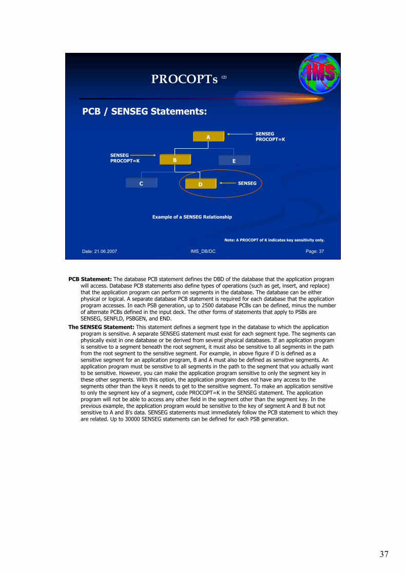
37
IMS_DB/DC Page: 37Date: 21.06.2007
PROCOPTs (2)
PCB / SENSEG Statements:
Example of a SENSEG Relationship
Note: A PROCOPT of K indicates key sensitivity only.
SENSEG PROCOPT=K
B
A
E
C D
SENSEG PROCOPT=K
SENSEG
PCB Statement: The database PCB statement defines the DBD of the database that the application program will access. Database PCB statements also define types of operations (such as get, insert, and replace) that the application program can perform on segments in the database. The database can be either physical or logical. A separate database PCB statement is required for each database that the application program accesses. In each PSB generation, up to 2500 database PCBs can be defined, minus the number of alternate PCBs defined in the input deck. The other forms of statements that apply to PSBs are SENSEG, SENFLD, PSBGEN, and END.
The SENSEG Statement: This statement defines a segment type in the database to which the application program is sensitive. A separate SENSEG statement must exist for each segment type. The segments can physically exist in one database or be derived from several physical databases. If an application program is sensitive to a segment beneath the root segment, it must also be sensitive to all segments in the path from the root segment to the sensitive segment. For example, in above figure if D is defined as a sensitive segment for an application program, B and A must also be defined as sensitive segments. An application program must be sensitive to all segments in the path to the segment that you actually want to be sensitive. However, you can make the application program sensitive to only the segment key in these other segments. With this option, the application program does not have any access to the segments other than the keys it needs to get to the sensitive segment. To make an application sensitive to only the segment key of a segment, code PROCOPT=K in the SENSEG statement. The application program will not be able to access any other field in the segment other than the segment key. In the previous example, the application program would be sensitive to the key of segment A and B but not sensitive to A and B’s data. SENSEG statements must immediately follow the PCB statement to which they are related. Up to 30000 SENSEG statements can be defined for each PSB generation.
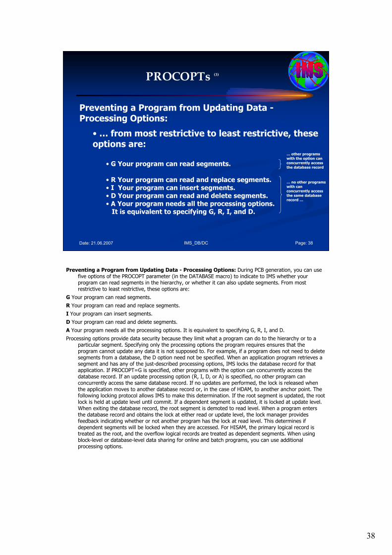
38
IMS_DB/DC Page: 38Date: 21.06.2007
PROCOPTs (3)
Preventing a Program from Updating Data -Processing Options:
•… from most restrictive to least restrictive, these options are:
• G Your program can read segments.
• R Your program can read and replace segments.• I Your program can insert segments. • D Your program can read and delete segments. • A Your program needs all the processing options. It is equivalent to specifying G, R, I, and D.
… other programs with the option can concurrently access the database record
… no other programs with can concurrently access the same database record …
Preventing a Program from Updating Data - Processing Options: During PCB generation, you can use five options of the PROCOPT parameter (in the DATABASE macro) to indicate to IMS whether your program can read segments in the hierarchy, or whether it can also update segments. From most restrictive to least restrictive, these options are:
G Your program can read segments.
R Your program can read and replace segments.
I Your program can insert segments.
D Your program can read and delete segments.
A Your program needs all the processing options. It is equivalent to specifying G, R, I, and D.
Processing options provide data security because they limit what a program can do to the hierarchy or to a particular segment. Specifying only the processing options the program requires ensures that the program cannot update any data it is not supposed to. For example, if a program does not need to delete segments from a database, the D option need not be specified. When an application program retrieves a segment and has any of the just-described processing options, IMS locks the database record for that application. If PROCOPT=G is specified, other programs with the option can concurrently access the database record. If an update processing option (R, I, D, or A) is specified, no other program can concurrently access the same database record. If no updates are performed, the lock is released when the application moves to another database record or, in the case of HDAM, to another anchor point. The following locking protocol allows IMS to make this determination. If the root segment is updated, the root lock is held at update level until commit. If a dependent segment is updated, it is locked at update level. When exiting the database record, the root segment is demoted to read level. When a program enters the database record and obtains the lock at either read or update level, the lock manager provides feedback indicating whether or not another program has the lock at read level. This determines if dependent segments will be locked when they are accessed. For HISAM, the primary logical record is treated as the root, and the overflow logical records are treated as dependent segments. When using block-level or database-level data sharing for online and batch programs, you can use additional processing options.
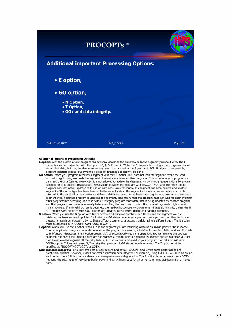
39
IMS_DB/DC Page: 39Date: 21.06.2007
PROCOPTs (3)
Additional important Processing Options:
• E option,
• GO option,
• N Option,• T Option,• GOx and data integrity.
Additional important Processing Options: E option: With the E option, your program has exclusive access to the hierarchy or to the segment you use it with. The E
option is used in conjunction with the options G, I, D, R, and A. While the E program is running, other programs cannot access that data, but may be able to access segments that are not in the E program’s PCB. No dynamic enqueue by program isolation is done, but dynamic logging of database updates will be done.
GO option: When your program retrieves a segment with the GO option, IMS does not lock the segment. While the read without integrity program reads the segment, it remains available to other programs. This is because your program can only read the data (termed read-only); it is not allowed to update the database. No dynamic enqueue is done by program isolation for calls against this database. Serialization between the program with PROCOPT=GO and any other update program does not occur; updates to the same data occur simultaneously. If a segment has been deleted and another segment of the same type has been inserted in the same location, the segment data and all subsequent data that is returned to the application may be from a different database record. A read-without-integrity program can also retrieve a segment even if another program is updating the segment. This means that the program need not wait for segments that other programs are accessing. If a read-without-integrity program reads data that is being updated by another program, and that program terminates abnormally before reaching the next commit point, the updated segments might contain invalid pointers. If an invalid pointer is detected, the read-without-integrity program terminates abnormally, unless the N or T options were specified with GO. Pointers are updated during insert, delete and backout functions.
N option: When you use the N option with GO to access a full-function database or a DEDB, and the segment you are retrieving contains an invalid pointer, IMS returns a GG status code to your program. Your program can then terminate processing, continue processing by reading a different segment, or access the data using a different path. The N option must be specified as PROCOPT=GON, GON, or GONP.
T option: When you use the T option with GO and the segment you are retrieving contains an invalid pointer, the response from an application program depends on whether the program is accessing a full-function or Fast Path database. For calls to full-function databases, the T option causes DL/I to automatically retry the operation. You can retrieve the updated segment, but only if the updating program has reached a commit point or has had its updates backed out since you last tried to retrieve the segment. If the retry fails, a GG status code is returned to your program. For calls to Fast Path DEDBs, option T does not cause DL/I to retry the operation. A GG status code is returned. The T option must be specified as PROCOPT=GOT, GOT, or GOTP.
GOx and data integrity: For a very small set of applications and data, PROCOPT=GOx offers some performance and parallelism benefits. However, it does not offer application data integrity. For example, using PROCOPT=GOT in an online environment on a full-function database can cause performance degradation. The T option forces a re-read from DASD, negating the advantage of very large buffer pools and VSAM hiperspace for all currently running applications and shared data.

40
IMS_DB/DC Page: 40Date: 21.06.2007
PROCOPTs (4)
PROCOPT GOx:
• Read Without Integrity,• Batch PGMs,• Online PGMs.
•What Read Without Integrity Means…
• Read-only (PROCOPT=GO) processing does not provide data integrity.
• Usage: eg. Reference DBs …• Performance Issue• GOx and data integrity…
Read Without Integrity: Database-level sharing of IMS databases provides for sharing of databases between a single update-capable batch or online IMS system and any number of other IMS systems that are reading data that are without integrity. A GE status code might be returned to a program using PROCOPT=GOx for a segment that exists in a HIDAM database during CI splits. In IMS, programs that use database-level sharing include PROCOPT=GOx in their DBPCBs for that data. For batch jobs, the DBPCB PROCOPTs establish the batch job’s access level for the database. That is, a batch job uses the highest declared intent for a database as the access level for DBRC database authorization. In an online IMS environment, database ACCESS is specified on the DATABASE macro during IMS system definition, and it can be changed using the /START DB ACCESS=RO command. Online IMS systems schedule programs with data availability determined by the PROCOPTs within those program PSBs being scheduled. That data availability is therefore limited by the online system’s database access. The PROCOPT=GON and GOT options provide certain limited PCB status code retry for some recognizable pointer errors, within the data that is being read without integrity. In some cases, dependent segment updates, occurring asynchronously to the read-without-integrity IMS instance, do not interfere with the program that is reading that data without integrity. However, update activity to an average database does not always allow a read-without-integrity IMS system to recognize a data problem.
What Read Without Integrity Means: Each IMS batch or online instance has OSAM and VSAM buffer pools defined for it. Without locking to serialize concurrent updates that are occurring in another IMS instance, a read without integrity from a database data set fetches a copy of a block or CI into the buffer pool in storage. Blocks or CIs in the buffer pool can remain there a long time. Subsequent read without integrity of other blocks or CIs can then fetch more recent data. Data hierarchies and other data relationships between these different blocks or CIs can be inconsistent. For example, consider an index database (VSAM KSDS), which has an index component and a data component. The index component contains only hierarchic control information, relating to the data component CI where a given keyed record is located. Think of this as the index component CI’s way of maintaining the high key in each data component CI. Inserting a keyed record into a KSDS data component CI that is already full causes a CI split. That is, some portion of the records in the existing CI are moved to a new CI, and the index component is adjusted to point to the new CI.
Hypothetical cases also exist where the deletion of a dependent segment and the insertion of that same segment type under a different root, placed in the same physical location as the deleted segment, can cause simple Get Next processing to give the appearance of only one root in the database. For example, accessing the segments under the first root in the database down to a level-06 segment (which had been deleted from the first root and is now logically under the last root) would then reflect data from the other root. The next and subsequent Get Next calls retrieve segments from the other root. Read-only (PROCOPT=GO) processing does not provide data integrity.
GOx and data integrity: For a very small set of applications and data, PROCOPT=GOx offers some performance and parallelism benefits. However, it does not offer application data integrity. For example, using PROCOPT=GOT in an online environment on a full-function database can cause performance degradation. The T option forces a re-read from DASD, negating the advantage of very large buffer pools and VSAM hiperspace for all currently running applications and shared data.

41
IMS_DB/DC Page: 41Date: 21.06.2007
PROCOPTs (5)
Complete List of PROCOPT Options:
see: IMS Utilities Reference
For a thorough description of the processing options see, last Version of IMS: Utilities Reference: System.
42
IMS_DB/DC Page: 42Date: 21.06.2007
Agenda Session 6: Data Sharing Issues
1. Integrity
2. Unit of Work
3. Commit Points / Sync Points
4. Locking
5. PROCOPTs
6.DL/I Calls
7. Deadlocks
8. Summary
6. DL/I Calls
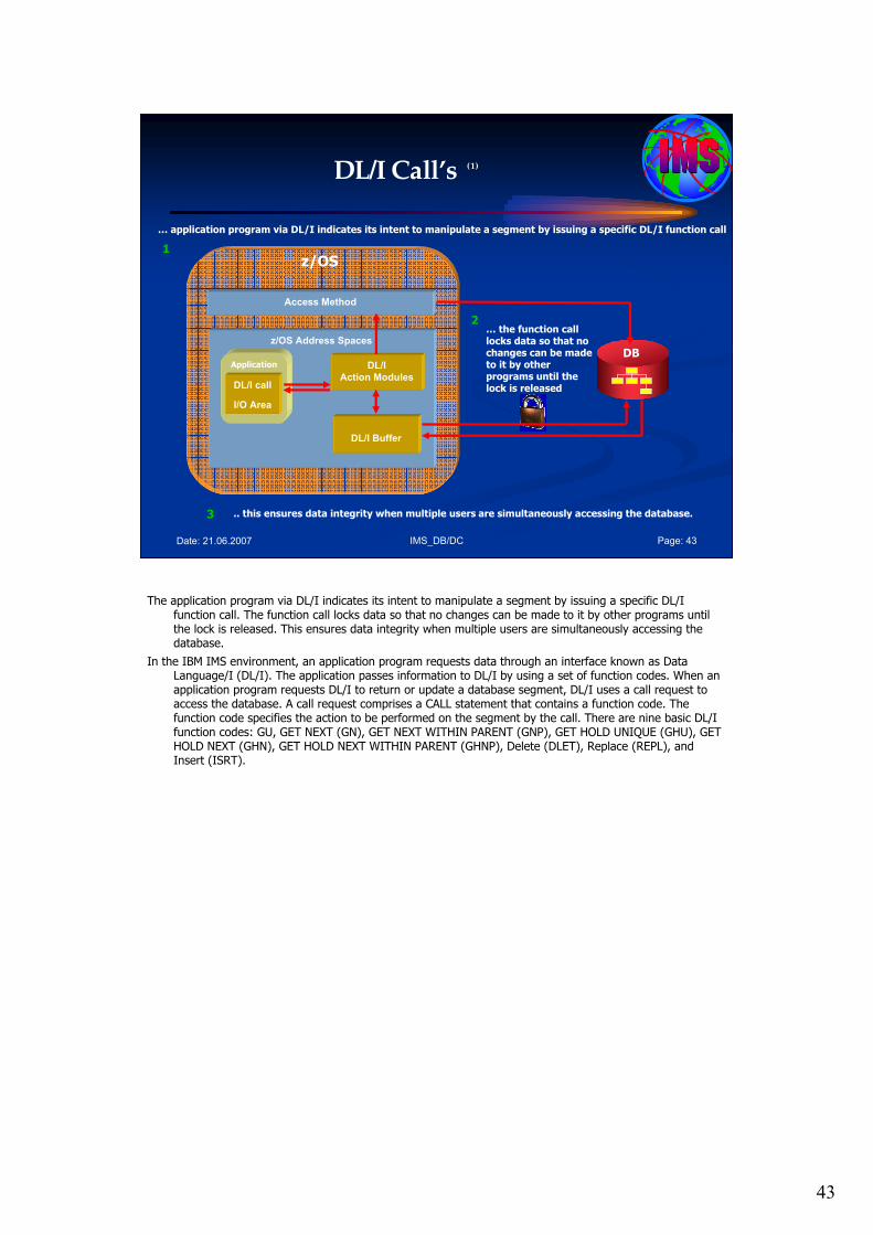
43
IMS_DB/DC Page: 43Date: 21.06.2007
DL/I Call’s (1)
DB
Access Method
z/OS Address Spaces
z/OS
Application
DL/I call
I/O Area
DL/I
Action Modules
DL/I Buffer
… application program via DL/I indicates its intent to manipulate a segment by issuing a specific DL/I function call
1
… the function call locks data so that no changes can be made to it by other programs until the lock is released
2
.. this ensures data integrity when multiple users are simultaneously accessing the database.3
The application program via DL/I indicates its intent to manipulate a segment by issuing a specific DL/I function call. The function call locks data so that no changes can be made to it by other programs until the lock is released. This ensures data integrity when multiple users are simultaneously accessing the database.
In the IBM IMS environment, an application program requests data through an interface known as Data Language/I (DL/I). The application passes information to DL/I by using a set of function codes. When an application program requests DL/I to return or update a database segment, DL/I uses a call request to access the database. A call request comprises a CALL statement that contains a function code. The function code specifies the action to be performed on the segment by the call. There are nine basic DL/I function codes: GU, GET NEXT (GN), GET NEXT WITHIN PARENT (GNP), GET HOLD UNIQUE (GHU), GET HOLD NEXT (GHN), GET HOLD NEXT WITHIN PARENT (GHNP), Delete (DLET), Replace (REPL), and Insert (ISRT).
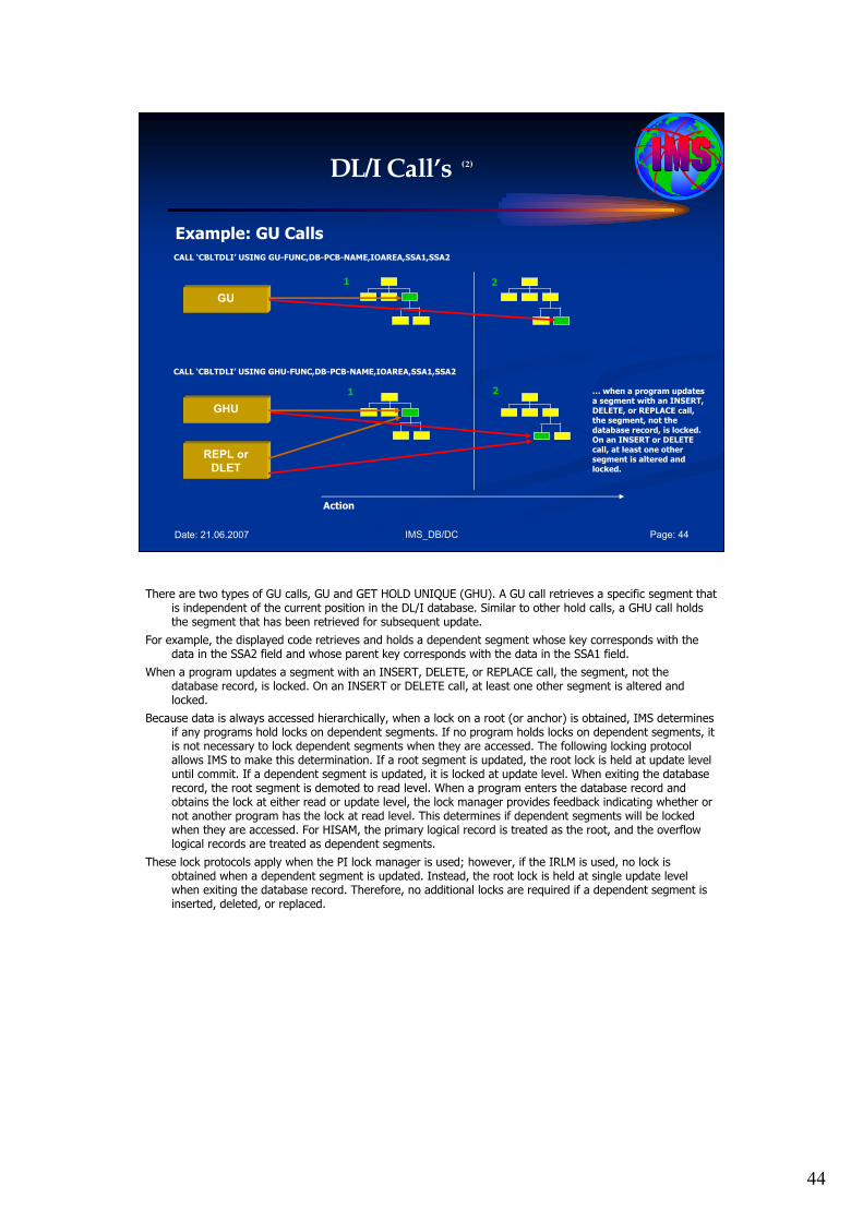
44
IMS_DB/DC Page: 44Date: 21.06.2007
DL/I Call’s (2)
Example: GU Calls
CALL ‘CBLTDLI’ USING GU-FUNC,DB-PCB-NAME,IOAREA,SSA1,SSA2
CALL ‘CBLTDLI’ USING GHU-FUNC,DB-PCB-NAME,IOAREA,SSA1,SSA2
GU
1 2
GHU
REPL or
DLET
1 2
Action
… when a program updates a segment with an INSERT, DELETE, or REPLACE call, the segment, not the database record, is locked. On an INSERT or DELETE call, at least one other segment is altered and locked.
There are two types of GU calls, GU and GET HOLD UNIQUE (GHU). A GU call retrieves a specific segment that is independent of the current position in the DL/I database. Similar to other hold calls, a GHU call holds the segment that has been retrieved for subsequent update.
For example, the displayed code retrieves and holds a dependent segment whose key corresponds with the data in the SSA2 field and whose parent key corresponds with the data in the SSA1 field.
When a program updates a segment with an INSERT, DELETE, or REPLACE call, the segment, not the database record, is locked. On an INSERT or DELETE call, at least one other segment is altered and locked.
Because data is always accessed hierarchically, when a lock on a root (or anchor) is obtained, IMS determines if any programs hold locks on dependent segments. If no program holds locks on dependent segments, it is not necessary to lock dependent segments when they are accessed. The following locking protocol allows IMS to make this determination. If a root segment is updated, the root lock is held at update level until commit. If a dependent segment is updated, it is locked at update level. When exiting the database record, the root segment is demoted to read level. When a program enters the database record and obtains the lock at either read or update level, the lock manager provides feedback indicating whether or not another program has the lock at read level. This determines if dependent segments will be locked when they are accessed. For HISAM, the primary logical record is treated as the root, and the overflow logical records are treated as dependent segments.
These lock protocols apply when the PI lock manager is used; however, if the IRLM is used, no lock is obtained when a dependent segment is updated. Instead, the root lock is held at single update level when exiting the database record. Therefore, no additional locks are required if a dependent segment is inserted, deleted, or replaced.
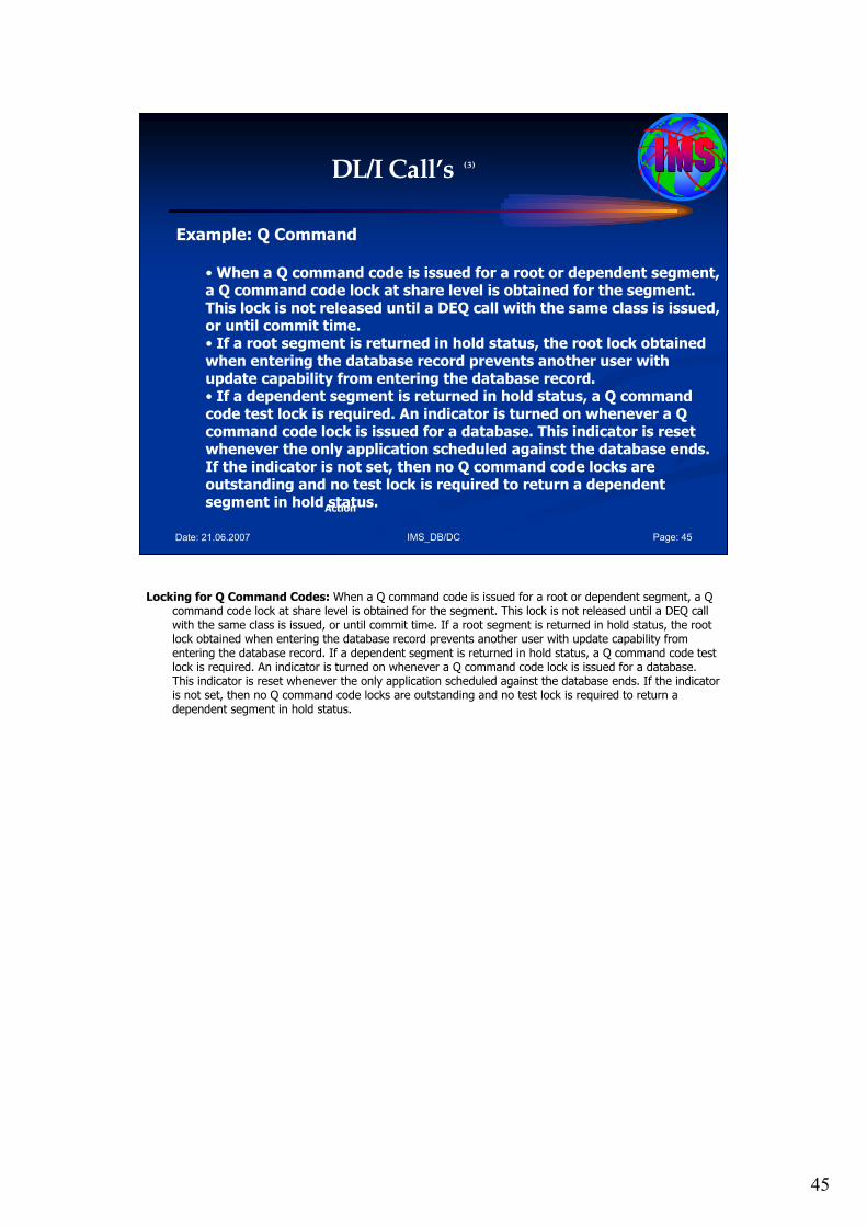
45
IMS_DB/DC Page: 45Date: 21.06.2007
DL/I Call’s (3)
Example: Q Command
•When a Q command code is issued for a root or dependent segment, a Q command code lock at share level is obtained for the segment. This lock is not released until a DEQ call with the same class is issued, or until commit time. • If a root segment is returned in hold status, the root lock obtained when entering the database record prevents another user with update capability from entering the database record. • If a dependent segment is returned in hold status, a Q command code test lock is required. An indicator is turned on whenever a Q command code lock is issued for a database. This indicator is reset whenever the only application scheduled against the database ends. If the indicator is not set, then no Q command code locks are outstanding and no test lock is required to return a dependent segment in hold status. Action
Locking for Q Command Codes: When a Q command code is issued for a root or dependent segment, a Q command code lock at share level is obtained for the segment. This lock is not released until a DEQ call with the same class is issued, or until commit time. If a root segment is returned in hold status, the root lock obtained when entering the database record prevents another user with update capability from entering the database record. If a dependent segment is returned in hold status, a Q command code test lock is required. An indicator is turned on whenever a Q command code lock is issued for a database. This indicator is reset whenever the only application scheduled against the database ends. If the indicator is not set, then no Q command code locks are outstanding and no test lock is required to return a dependent segment in hold status.

46
IMS_DB/DC Page: 46Date: 21.06.2007
Agenda Session 6: Data Sharing Issues
1. Integrity
2. Unit of Work
3. Commit Points / Sync Points
4. Locking
5. PROCOPTs
6. DL/I Calls
7.Deadlocks
8. Summary
7. Deadlocks
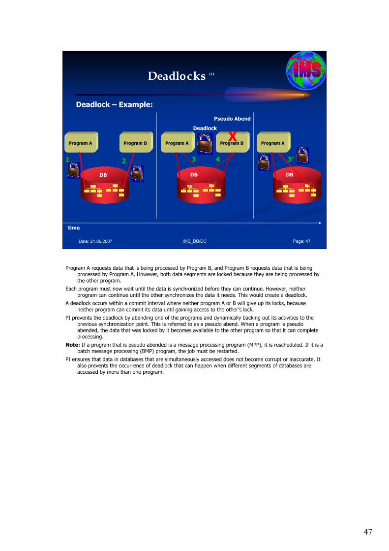
47
IMS_DB/DC Page: 47Date: 21.06.2007
Deadlocks (1)
Program A Program B
DB
2
Program A Program B
DB
3 4
time
X
Pseudo Abend
Deadlock
Deadlock – Example:
Program A
DB
1 3’
Program A requests data that is being processed by Program B, and Program B requests data that is being processed by Program A. However, both data segments are locked because they are being processed by the other program.
Each program must now wait until the data is synchronized before they can continue. However, neither program can continue until the other synchronizes the data it needs. This would create a deadlock.
A deadlock occurs within a commit interval where neither program A or B will give up its locks, because neither program can commit its data until gaining access to the other’s lock.
PI prevents the deadlock by abending one of the programs and dynamically backing out its activities to the previous synchronization point. This is referred to as a pseudo abend. When a program is pseudo abended, the data that was locked by it becomes available to the other program so that it can complete processing.
Note: If a program that is pseudo abended is a message processing program (MPP), it is rescheduled. If it is a batch message processing (BMP) program, the job must be restarted.
PI ensures that data in databases that are simultaneously accessed does not become corrupt or inaccurate. It also prevents the occurrence of deadlock that can happen when different segments of databases are accessed by more than one program.
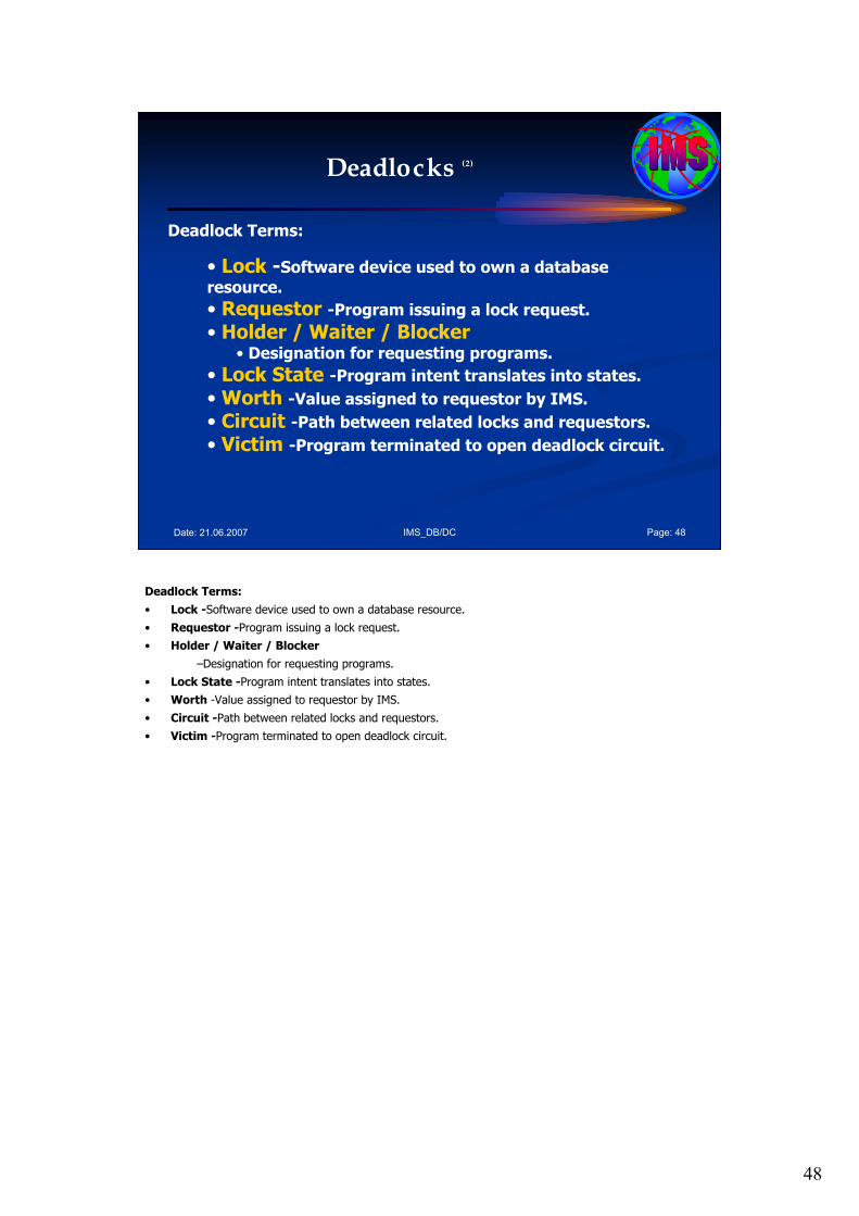
48
IMS_DB/DC Page: 48Date: 21.06.2007
Deadlocks (2)
Deadlock Terms:
• Lock -Software device used to own a database resource.
• Requestor -Program issuing a lock request.• Holder / Waiter / Blocker
• Designation for requesting programs.
• Lock State -Program intent translates into states.
•Worth -Value assigned to requestor by IMS.
• Circuit -Path between related locks and requestors.• Victim -Program terminated to open deadlock circuit.
Deadlock Terms:
• Lock -Software device used to own a database resource.
• Requestor -Program issuing a lock request.
• Holder / Waiter / Blocker
–Designation for requesting programs.
• Lock State -Program intent translates into states.
• Worth -Value assigned to requestor by IMS.
• Circuit -Path between related locks and requestors.
• Victim -Program terminated to open deadlock circuit.
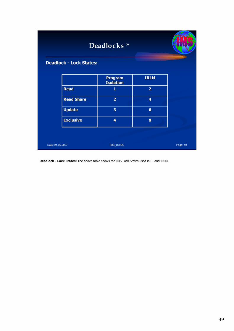
49
IMS_DB/DC Page: 49Date: 21.06.2007
Deadlocks (3)
Deadlock - Lock States:
8844ExclusiveExclusive
6633UpdateUpdate
4422Read ShareRead Share
2211ReadRead
IRLMIRLMProgram Program
IsolationIsolation
Deadlock - Lock States: The above table shows the IMS Lock States used in PI and IRLM.
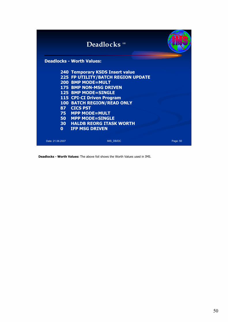
50
IMS_DB/DC Page: 50Date: 21.06.2007
Deadlocks (4)
Deadlocks - Worth Values:
240 Temporary KSDS Insert value 225 FP UTILITY/BATCH REGION UPDATE 200 BMP MODE=MULT 175 BMP NON-MSG DRIVEN 125 BMP MODE=SINGLE 115 CPI-CI Driven Program 100 BATCH REGION/READ ONLY 87 CICS PST 75 MPP MODE=MULT 50 MPP MODE=SINGLE 30 HALDB REORG ITASK WORTH 0 IFP MSG DRIVEN
Deadlocks - Worth Values: The above foil shows the Worth Values used in IMS.
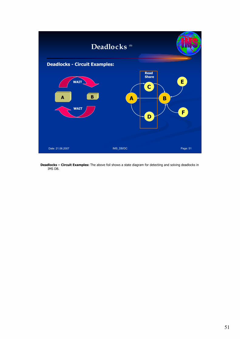
51
IMS_DB/DC Page: 51Date: 21.06.2007
Deadlocks (5)
Deadlocks - Circuit Examples:
A B
WAIT
WAIT
A B
D
CE
F
ReadShare
Deadlocks – Circuit Examples: The above foil shows a state diagram for detecting and solving deadlocks in IMS DB.
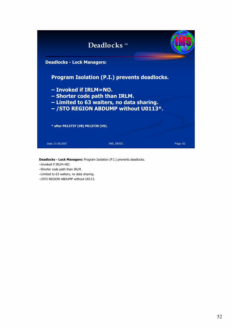
52
IMS_DB/DC Page: 52Date: 21.06.2007
Deadlocks (6)
Deadlocks - Lock Managers:
Program Isolation (P.I.) prevents deadlocks.
– Invoked if IRLM=NO. – Shorter code path than IRLM. – Limited to 63 waiters, no data sharing.– /STO REGION ABDUMP without U0113*.
* after PK13737 (V8) PK13739 (V9).
Deadlocks - Lock Managers: Program Isolation (P.I.) prevents deadlocks.
–Invoked if IRLM=NO.
–Shorter code path than IRLM.
–Limited to 63 waiters, no data sharing.
–/STO REGION ABDUMP without U0113.
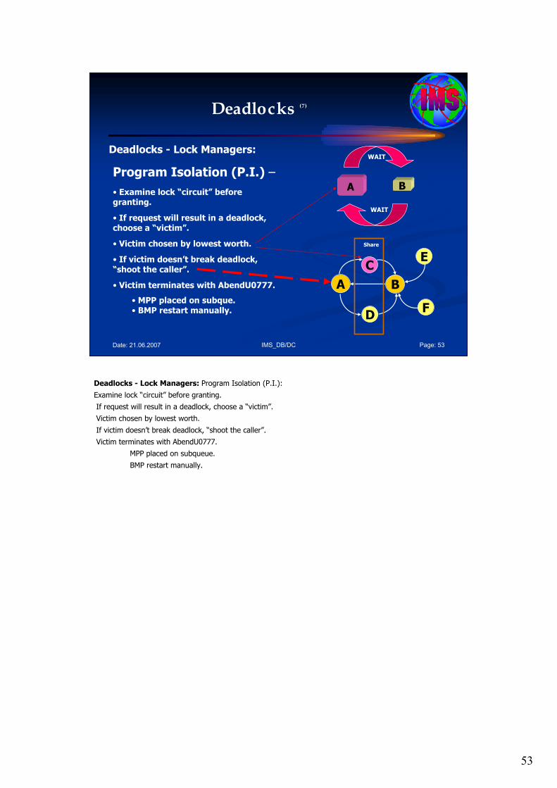
53
IMS_DB/DC Page: 53Date: 21.06.2007
Deadlocks (7)
Deadlocks - Lock Managers:
Program Isolation (P.I.) –
• Examine lock “circuit” before granting.
• If request will result in a deadlock, choose a “victim”.
• Victim chosen by lowest worth.
• If victim doesn’t break deadlock, “shoot the caller”.
• Victim terminates with AbendU0777.
• MPP placed on subque. • BMP restart manually.
A B
WAIT
WAIT
A B
D
CE
F
Share
Deadlocks - Lock Managers: Program Isolation (P.I.):
Examine lock “circuit” before granting.
If request will result in a deadlock, choose a “victim”.
Victim chosen by lowest worth.
If victim doesn’t break deadlock, “shoot the caller”.
Victim terminates with AbendU0777.
MPP placed on subqueue.
BMP restart manually.
54
IMS_DB/DC Page: 54Date: 21.06.2007
Deadlocks (8)
Deadlocks - Lock Managers:
IRLM - Resolves Deadlocks
– Multiple IMS’s, supports Sysplex Data Sharing group.– Multiple IRLM’s (one per z/OS image per group).– Greater availability.
• An IRLM outage doesn’t cripple entire system.• Sharing IRLMs retain failing IRLM’s locks.
– Use “LOCKTIME” to safely end waiters w/o U0113.
Deadlocks - Lock Managers: IRLM - Resolves Deadlocks
–Multiple IMS’s, supports Sysplex Data Sharing group.
–Multiple IRLM’s (one per z/OS image per group).
–Greater availability.
• An IRLM outage doesn’t cripple entire system.
• Sharing IRLMs retain failing IRLM’s locks.
–Use “LOCKTIME” to safely end waiters w/o U0113.
55
IMS_DB/DC Page: 55Date: 21.06.2007
Deadlocks (9)
Deadlocks - Lock Managers:
IRLM Deadlock Resolution process
– IRLM Deadlock Manager collects information.• Once per IRLM Deadlock cycle.
– IRLM passes info to IMS Deadlock exit.– Deadlock exit chooses “victim”.– IRLM resumes victim’s request with lock reject.– IMS terminates victim with ABENDU0777.
Deadlocks - Lock Managers: IRLM - Resolves Deadlocks:
IRLM Deadlock Resolution process:
– IRLM Deadlock Manager collects information.
• Once per IRLM Deadlock cycle.
– IRLM passes info to IMS Deadlock exit.
– Deadlock exit chooses “victim”.
– IRLM resumes victim’s request with lock reject.
– IMS terminates victim with ABENDU0777.
56
IMS_DB/DC Page: 56Date: 21.06.2007
Deadlocks (10)
Deadlocks - Lock Managers:
IRLM Deadlock Cycle time controlled by:
– DXRJPROC JCL parm“DEADLOCK=(s,n)“
• “s” = time between cycles, can be under a second.»1 -> 100 = seconds »101 -> 5000 = milliseconds
•“n” = number of “local” cycles before “global” cycle.
Deadlocks - Lock Managers: IRLM Deadlock Cycle time is controlled by a JCL parameter DEADLOCK.
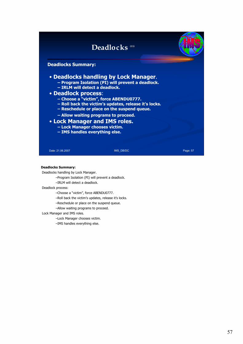
57
IMS_DB/DC Page: 57Date: 21.06.2007
Deadlocks (11)
Deadlocks Summary:
• Deadlocks handling by Lock Manager. – Program Isolation (PI) will prevent a deadlock.– IRLM will detect a deadlock.
• Deadlock process:– Choose a “victim”, force ABENDU0777.– Roll back the victim’s updates, release it’s locks.– Reschedule or place on the suspend queue.
– Allow waiting programs to proceed.
• Lock Manager and IMS roles.– Lock Manager chooses victim.– IMS handles everything else.
Deadlocks Summary:
Deadlocks handling by Lock Manager.
–Program Isolation (PI) will prevent a deadlock.
–IRLM will detect a deadlock.
Deadlock process:
–Choose a “victim”, force ABENDU0777.
–Roll back the victim’s updates, release it’s locks.
–Reschedule or place on the suspend queue.
–Allow waiting programs to proceed.
Lock Manager and IMS roles.
–Lock Manager chooses victim.
–IMS handles everything else.

58
IMS_DB/DC Page: 58Date: 21.06.2007
Agenda Session 6: Data Sharing Issues
1. Integrity
2. Unit of Work
3. Commit Points / Sync Points
4. Locking
5. PROCOPTs
6. DL/I Calls
7. Deadlocks
8. Summary
8. Summary
59
IMS_DB/DC Page: 59Date: 21.06.2007
Summary
• You control how an application program views your database.
• An application program might not need use of all the segments or fields in a database record.
• And an application program may not need access to specific segments for security or integrity purposes.
• An application program may not need to perform certain types of operations on some segments or fields.
• You control which segments and fields an application can view and which operations it can perform on a segment by coding and generating a PSB.
• Even DL/I call functions influence locking mechanism.
You control how an application program views your database. An application program might not need use of all the segments or fields in a database record. And an application program may not need access to specific segments for security or integrity purposes. An application program may not need to perform certain types of operations on some segments or fields. For example, an application program needs read access to a SALARY segment but not update access. You control which segments and fields an application can view and which operations it can perform on a segment by coding and generating a PSB (program specification block).
Even DL/I call functions influence locking mechanism.

60
IMS_DB/DC Page: 60Date: 21.06.2007
Source
See: • IBM Web page
http://www-306.ibm.com/software/data/ims/
• BookAn Introduction to IMS, IBM Press
In all sessions I like to motivate you to study additional books and publications about IMS DB/DC.

61
Date: 21.06.2007 IMS_03_6.ppt Page: 61
Questions / CommentsQuestions / Comments……
? ? ?? ? ?
Questions, comments, further information?
Please feel free to e-mail me!
Dipl.Ing. Werner HoffmannDipl.Ing. Werner Hoffmann
EMAIL: EMAIL: pwhoffmann@[email protected]
The time for this session is over. If you have additional questions or comments or like to get further information please feel free to e mail me at [email protected] or [email protected].

62
IMS_DB/DC Page: 62Date: 21.06.2007
The End…
Part III/6: IMS Hierarchical Database ModelIMS Hierarchical Database Model
Data Sharing IssuesData Sharing Issues
Workshop
The world depends on it
I hope this presentation was right for you! Enjoy the following discussion!

1
Date: 21.06.2007 IMS_03_7.ppt Page: 1
IBM Mainframe
IMS DB/DC
Database Design Workshop
Part III: Part III:
IMS Hierarchical Database ModelIMS Hierarchical Database ModelSession 7: Session 7: Implementing IMS DatabasesImplementing IMS Databases
May 2007 May 2007 –– 1st Version1st Version
presented bypresented by
Dipl. Dipl. IngIng. Werner Hoffmann. Werner HoffmannEMAIL: EMAIL: pwhoffmann @ tpwhoffmann @ t--online.deonline.de
A member of IEEE and ACM
Mainframe
Please see the notes pages for additional comments. Please see the notes pages for additional comments.
Welcome to the workshop called “IMS DB/DC". This is part 3: IMS Hierarchical Database Model – Session 5: Implementing IMS Databases.
2
IMS_DB/DC Page: 2Date: 21.06.2007
Agenda
Session 7: Implementing IMS Databases
1. Basic Terms
2. DBDGEN
• Physical DB’s
• Logical DB’s
3. PSBGEN
4. ACBGEN
Here is the Agenda for the IMS DB/DC workshop part III/7: Implementing IMS Databases.
In this session I like to speak about:
1. Basic Terms
2. DBDGEN
• Physical DB’s
• Logical DB’s
3. PSBGEN
4. ACBGEN
3
IMS_DB/DC Page: 3Date: 21.06.2007
Agenda
Session 7: Implementing IMS Databases
1. Basic Terms
2. DBDGEN
• Physical DB’s
• Logical DB’s
3. PSBGEN
4. ACBGEN
1. Basic Terms

4
IMS_DB/DC Page: 4Date: 21.06.2007
Basics (1)
Implementing Database Design:
• DBDGEN (database description)• physical and logical characteristics
• PSBGEN (program specification)
• ACBGEN (application control block)• special internal format • DBD and PSB information
Implementing Database Design After you have designed your databases and before application programs can use them, you must tell IMS their physical and logical characteristics by coding and generating a DBD (database description) for each database. Before an application program can use the database, you must tell IMS the application program’s characteristics and use of data and terminals. You tell IMS the application program characteristics by coding and generating a PSB (program specification block). Finally, before an application program can be scheduled for execution, IMS needs the PSB and DBD information for the application program available in a special internal format called an ACB (application control block).
5
IMS_DB/DC Page: 5Date: 21.06.2007
Basics (2)
Implementing Database Design:
• … for more details see:
• dfsadbg3.pdf – IMS Administration Guide: Database Manager
• dfsursg3.pdf – IMS Utilities Reference: System
Note: Only a small part will be discussed in this session!
In this session I will give only initial information about the three needed steps: DBDGEN, PSBGEN and ACBGEN. For more details please refer to the IBM manuals, specially:
• dfsadbg3.pdf – IMS Administration Guide: Database Manager,
• dfsursg3.pdf – IMS Utilities Reference: System.

6
IMS_DB/DC Page: 6Date: 21.06.2007
Agenda
Session 7: Implementing IMS Databases
1. Basic Terms
2. DBDGEN
• Physical DB’s
• Logical DB’s
3. PSBGEN
4. ACBGEN
2. DBDGEN
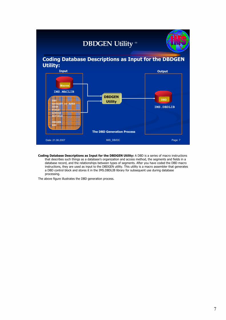
7
IMS_DB/DC Page: 7Date: 21.06.2007
DBDGEN Utility (1)
Coding Database Descriptions as Input for the DBDGEN Utility:
Macros
IMS.MACLIB
IMS.DBDLIB
DBD
DATASET or AREA
SEGM
FIELD
LCHILD
XDFIELD
…
DBDGEN
END
DBDDBDGEN
Utility
The DBD Generation Process
Input Output
Coding Database Descriptions as Input for the DBDGEN Utility: A DBD is a series of macro instructions that describes such things as a database’s organization and access method, the segments and fields in a database record, and the relationships between types of segments. After you have coded the DBD macro instructions, they are used as input to the DBDGEN utility. This utility is a macro assembler that generates a DBD control block and stores it in the IMS.DBDLIB library for subsequent use during database processing.
The above figure illustrates the DBD generation process.
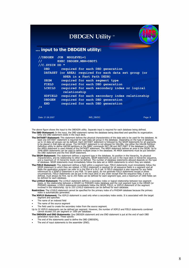
8
IMS_DB/DC Page: 8Date: 21.06.2007
DBDGEN Utility (2)
… input to the DBDGEN utility:
//DBDGEN JOB MSGLEVEL=1
// EXEC DBDGEN,MBR=DBDT1
//C.SYSIN DD *
DBD required for each DBD generation
DATASET (or AREA) required for each data set group (or
AREA in a Fast Path DEDB)
SEGM required for each segment type
FIELD required for each DBD generation
LCHILD required for each secondary index or logical
relationship
XDFIELD required for each secondary index relationship
DBDGEN required for each DBD generation
END required for each DBD generation
/*
The above figure shows the input to the DBDGEN utility. Separate input is required for each database being defined.
The DBD Statement: In the input, the DBD statement names the database being described and specifies its organization. Only one DBD statement exists in the input deck.
The DATASET Statement: This statement defines the physical characteristics of the data sets to be used for the database. At least one DATASET statement is required for each data set group in the database. Depending on the type of database, up to 10 data set groups can be defined. Each DATASET statement is followed by the SEGM statements for all segments to be placed in that data set group. The DATASET statement is not allowed for HALDBs. Use either the HALDB Partition Definition utility to define HALDB partitions or the DBRC commands INIT.DB and INIT.PART If the database is a DEDB, the AREA statement is used instead of the DATASET statement. The AREA statement defines an area in the DEDB. Up to 2048 AREA statements can be used to define multiple areas in the database. All AREA statements must be put between the DBD statement and the first SEGM statement.
The SEGM Statement: This statement defines a segment type in the database, its position in the hierarchy, its physical characteristics, and its relationship to other segments. SEGM statements are put in the input deck in hierarchic sequence, and a maximum of 15 hierarchic levels can be defined. The number of database statements allowed depends on the type of database. SEGM statements must immediately follow the data set or AREA statements to which they are related.
The FIELD Statement: This statement defines a field within a segment type. FIELD statements must immediately follow the SEGM statement to which they are related. A FIELD statement is required for all sequence fields in a segment and all fields the application program can refer to in the SSA of a DL/I call. A FIELD statement is also required for any fields referenced by a SENFLD statement in any PSB. To save space, do not generate FIELD statements except in these circumstances. FIELD statements can be put in the input deck in any order except that the sequence field, if one is defined, must always be first. Up to 255 fields can be defined for each segment type, and a maximum of 1000 fields can be defined for each database.
The LCHILD Statement: The LCHILD statement defines a secondary index or logical relationship between two segment types, or the relationship between a HIDAM (or PHIDAM) index database and the root segment type in the HIDAM (or PHIDAM) database. LCHILD statements immediately follow the SEGM, FIELD, or XDFLD statement of the segment involved in the relationship. Up to 255 LCHILD statements can be defined for each database.
Restriction: The LCHILD statement cannot be specified for the primary index of a PHIDAM database because the primary index is automatically generated.
The XDFLD Statement: The XDFLD statement is used only when a secondary index exists. It is associated with the target segment and specifies:
• The name of an indexed field
• The name of the source segment
• The field used to create the secondary index from the source segment.
Up to 32 XDFLD statements can be defined per segment. However, the number of XDFLD and FIELD statements combined cannot exceed 255 per segment or 1000 per database.
The DBDGEN and END Statements: One DBDGEN statement and one END statement is put at the end of each DBD generation input deck. These specify:
• The end of the statements used to define the DBD (DBDGEN),
• The end of input statements to the assembler (END).
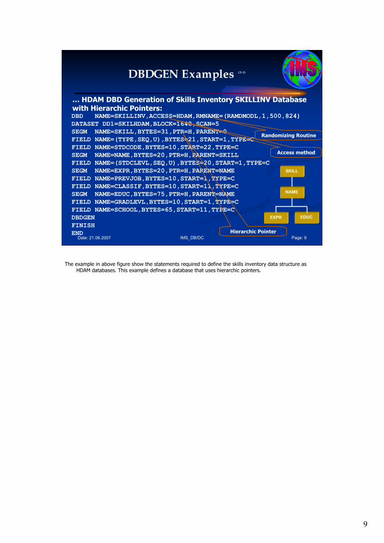
9
IMS_DB/DC Page: 9Date: 21.06.2007
DBDGEN Examples (3-1)
… HDAM DBD Generation of Skills Inventory SKILLINV Database with Hierarchic Pointers:DBD NAME=SKILLINV,ACCESS=HDAM,RMNAME=(RAMDMODL,1,500,824)
DATASET DD1=SKILHDAM,BLOCK=1648,SCAN=5
SEGM NAME=SKILL,BYTES=31,PTR=H,PARENT=0
FIELD NAME=(TYPE,SEQ,U),BYTES=21,START=1,TYPE=C
FIELD NAME=STDCODE,BYTES=10,START=22,TYPE=C
SEGM NAME=NAME,BYTES=20,PTR=H,PARENT=SKILL
FIELD NAME=(STDCLEVL,SEQ,U),BYTES=20,START=1,TYPE=C
SEGM NAME=EXPR,BYTES=20,PTR=H,PARENT=NAME
FIELD NAME=PREVJOB,BYTES=10,START=1,TYPE=C
FIELD NAME=CLASSIF,BYTES=10,START=11,TYPE=C
SEGM NAME=EDUC,BYTES=75,PTR=H,PARENT=NAME
FIELD NAME=GRADLEVL,BYTES=10,START=1,TYPE=C
FIELD NAME=SCHOOL,BYTES=65,START=11,TYPE=C
DBDGEN
FINISH
END
SKILL
NAME
EXPR EDUC
Access method
Randomizing Routine
Hierarchic Pointer
The example in above figure show the statements required to define the skills inventory data structure as HDAM databases. This example defines a database that uses hierarchic pointers.
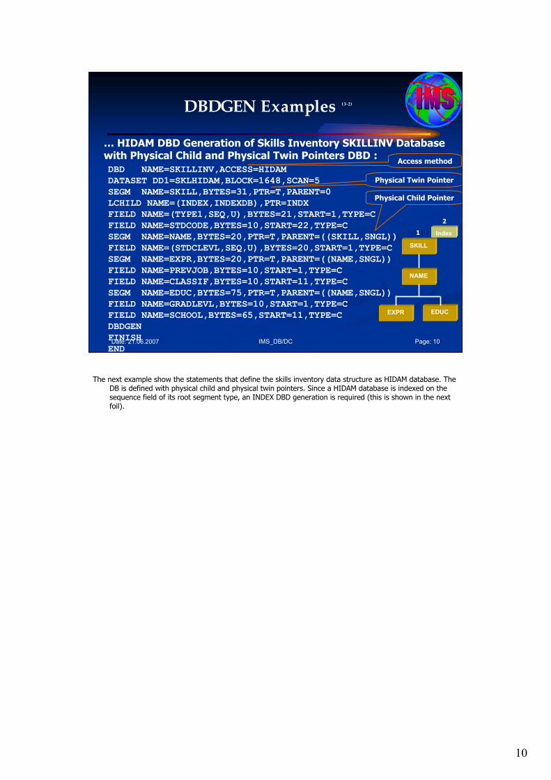
10
IMS_DB/DC Page: 10Date: 21.06.2007
DBDGEN Examples (3-2)
… HIDAM DBD Generation of Skills Inventory SKILLINV Database with Physical Child and Physical Twin Pointers DBD :
DBD NAME=SKILLINV,ACCESS=HIDAM
DATASET DD1=SKLHIDAM,BLOCK=1648,SCAN=5
SEGM NAME=SKILL,BYTES=31,PTR=T,PARENT=0
LCHILD NAME=(INDEX,INDEXDB),PTR=INDX
FIELD NAME=(TYPE1,SEQ,U),BYTES=21,START=1,TYPE=C
FIELD NAME=STDCODE,BYTES=10,START=22,TYPE=C
SEGM NAME=NAME,BYTES=20,PTR=T,PARENT=((SKILL,SNGL))
FIELD NAME=(STDCLEVL,SEQ,U),BYTES=20,START=1,TYPE=C
SEGM NAME=EXPR,BYTES=20,PTR=T,PARENT=((NAME,SNGL))
FIELD NAME=PREVJOB,BYTES=10,START=1,TYPE=C
FIELD NAME=CLASSIF,BYTES=10,START=11,TYPE=C
SEGM NAME=EDUC,BYTES=75,PTR=T,PARENT=((NAME,SNGL))
FIELD NAME=GRADLEVL,BYTES=10,START=1,TYPE=C
FIELD NAME=SCHOOL,BYTES=65,START=11,TYPE=C
DBDGEN
FINISH
END
Access method
Physical Twin Pointer
Physical Child Pointer
SKILL
NAME
EXPR EDUC
Index1
2
The next example show the statements that define the skills inventory data structure as HIDAM database. The DB is defined with physical child and physical twin pointers. Since a HIDAM database is indexed on the sequence field of its root segment type, an INDEX DBD generation is required (this is shown in the next foil).
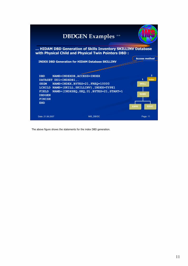
11
IMS_DB/DC Page: 11Date: 21.06.2007
DBDGEN Examples (3-3)
… HIDAM DBD Generation of Skills Inventory SKILLINV Database with Physical Child and Physical Twin Pointers DBD :
Access method
SKILL
NAME
EXPR EDUC
Index1
2DBD NAME=INDEXDB,ACCESS=INDEX
DATASET DD1=INDXDB1,…
SEGM NAME=INDEX,BYTES=21,FREQ=10000
LCHILD NAME=(SKILL,SKILLINV),INDEX=TYPE1
FIELD NAME=(INDXSEQ,SEQ,U),BYTES=21,START=1
DBDGEN
FINISH
END
INDEX DBD Generation for HIDAM Database SKILLINV
The above figure shows the statements for the index DBD generation.

12
IMS_DB/DC Page: 12Date: 21.06.2007
DBDGEN (4)
… Specifying Rules in the Physical DBD:
Insert Delete Replace
Insert, Delete, and Replace Rules in the DBD
B Specifies a bidirectional virtual delete rule. L Specifies a logical insert, delete, or replace rule. P Specifies a physical insert, delete, or replace rule. V Specifies a virtual insert, delete, or replace rule.
SEGM other parameters RULES=( P , P , P )
L L L
V V V
B
Understanding Syntax Diagrams (1)
… Specifying Rules in the Physical DBD: Insert, delete, and replace rules are specified using the RULES=keyword of a SEGM statement in the DBD for logical relationships. The above figure contains a diagram of the RULES= keyword and its parameters.
The valid parameter values for the RULES= keyword are:
B Specifies a bidirectional virtual delete rule. It is not a valid value for either the first or last positional parameter of the RULES= keyword.
L Specifies a logical insert, delete, or replace rule.
P Specifies a physical insert, delete, or replace rule.
V Specifies a virtual insert, delete, or replace rule.
The RULES= keyword accepts three positional parameters:
• The first positional parameter sets the insert rule
• The second positional parameter sets the delete rule
• The third positional parameter sets the replace rule.
For example, RULES=P,L,V says the insert rule is physical, the delete rule is logical, and the replace rule is virtual. The B rule is only applicable for delete. In general, the P rule is the most restrictive, the V rule is least restrictive, and the L rule is somewhere in between.
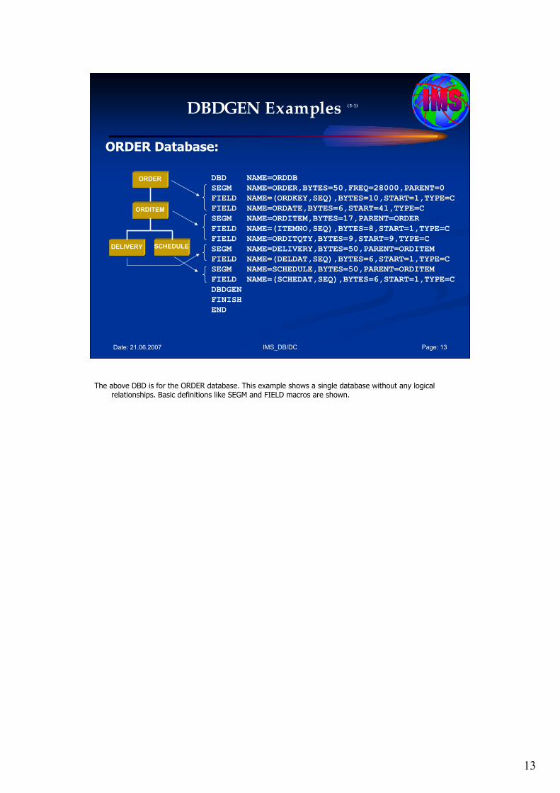
13
IMS_DB/DC Page: 13Date: 21.06.2007
DBDGEN Examples (5-1)
ORDER Database:
DBD NAME=ORDDB
SEGM NAME=ORDER,BYTES=50,FREQ=28000,PARENT=0
FIELD NAME=(ORDKEY,SEQ),BYTES=10,START=1,TYPE=C
FIELD NAME=ORDATE,BYTES=6,START=41,TYPE=C
SEGM NAME=ORDITEM,BYTES=17,PARENT=ORDER
FIELD NAME=(ITEMNO,SEQ),BYTES=8,START=1,TYPE=C
FIELD NAME=ORDITQTY,BYTES=9,START=9,TYPE=C
SEGM NAME=DELIVERY,BYTES=50,PARENT=ORDITEM
FIELD NAME=(DELDAT,SEQ),BYTES=6,START=1,TYPE=C
SEGM NAME=SCHEDULE,BYTES=50,PARENT=ORDITEM
FIELD NAME=(SCHEDAT,SEQ),BYTES=6,START=1,TYPE=C
DBDGEN
FINISH
END
ORDER
ORDITEM
DELIVERY SCHEDULE
The above DBD is for the ORDER database. This example shows a single database without any logical relationships. Basic definitions like SEGM and FIELD macros are shown.
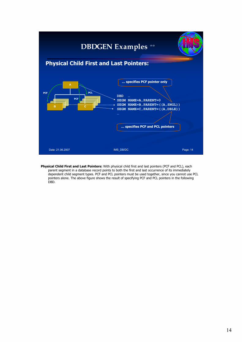
14
IMS_DB/DC Page: 14Date: 21.06.2007
DBDGEN Examples (5-2)
Physical Child First and Last Pointers:
DBD …
SEGM NAME=A,PARENT=0
SEGM NAME=B,PARENT=((A,SNGL))
SEGM NAME=C,PARENT=((A,DBLE))
…
BB
A
B C
PCF
PCF
PCL
… specifies PCF pointer only
… specifies PCF and PCL pointers
Physical Child First and Last Pointers: With physical child first and last pointers (PCF and PCL), each parent segment in a database record points to both the first and last occurrence of its immediately dependent child segment types. PCF and PCL pointers must be used together, since you cannot use PCL pointers alone. The above figure shows the result of specifying PCF and PCL pointers in the following DBD.
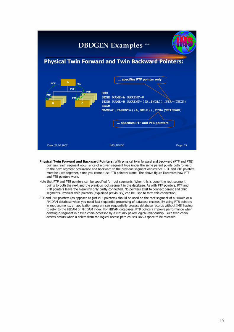
15
IMS_DB/DC Page: 15Date: 21.06.2007
DBDGEN Examples (5-3)
Physical Twin Forward and Twin Backward Pointers:
DBD …
SEGM NAME=A,PARENT=0
SEGM NAME=B,PARENT=((A,SNGL)),PTR=(TWIN)
SEGM
NAME=C,PARENT=((A,DBLE)),PTR=(TWINBWD)
…
… specifies PTF pointer only
… specifies PTF and PFB pointers
BB
A
B C
PCF
PCF
PCL
PTF
PTF
PTB
Physical Twin Forward and Backward Pointers: With physical twin forward and backward (PTF and PTB) pointers, each segment occurrence of a given segment type under the same parent points both forward to the next segment occurrence and backward to the previous segment occurrence. PTF and PTB pointers must be used together, since you cannot use PTB pointers alone. The above figure illustrates how PTF and PTB pointers work.
Note that PTF and PTB pointers can be specified for root segments. When this is done, the root segment points to both the next and the previous root segment in the database. As with PTF pointers, PTF and PTB pointers leave the hierarchy only partly connected. No pointers exist to connect parent and child segments. Physical child pointers (explained previously) can be used to form this connection.
PTF and PTB pointers (as opposed to just PTF pointers) should be used on the root segment of a HIDAM or a PHIDAM database when you need fast sequential processing of database records. By using PTB pointers in root segments, an application program can sequentially process database records without IMS’ having to refer to the HIDAM or PHIDAM index. For HIDAM databases, PTB pointers improve performance when deleting a segment in a twin chain accessed by a virtually paired logical relationship. Such twin-chain access occurs when a delete from the logical access path causes DASD space to be released.
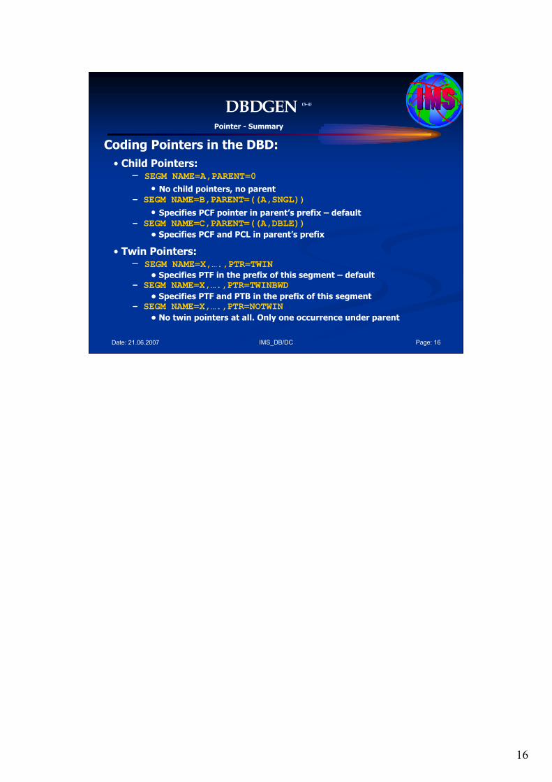
16
IMS_DB/DC Page: 16Date: 21.06.2007
DBDGEN (5-4)
Coding Pointers in the DBD:
• Child Pointers:– SEGM NAME=A,PARENT=0
• No child pointers, no parent
– SEGM NAME=B,PARENT=((A,SNGL))
• Specifies PCF pointer in parent’s prefix – default
– SEGM NAME=C,PARENT=((A,DBLE))
• Specifies PCF and PCL in parent’s prefix
• Twin Pointers:– SEGM NAME=X,….,PTR=TWIN
• Specifies PTF in the prefix of this segment – default– SEGM NAME=X,….,PTR=TWINBWD
• Specifies PTF and PTB in the prefix of this segment– SEGM NAME=X,….,PTR=NOTWIN
• No twin pointers at all. Only one occurrence under parent
Pointer - Summary

17
IMS_DB/DC Page: 17Date: 21.06.2007
DBDGEN (5-5)
Coding Pointers in the DBD:
• Hierarchic Pointers:
– SEGM NAME=Y,….,PTR=HIER
• Specifies HF pointer in the prefix of this segment
– SEGM NAME=Y,….,PTR=HIERBWD
• Specifies HF and HB pointers in the prefix of this segment
Pointer - Summary

18
IMS_DB/DC Page: 18Date: 21.06.2007
DBDGEN Examples (6-1)
Fixed- and Variable-Length Segments:
Defining a Variable-Length Segment:
ROOTSEG SEGM NAME=ROOTSEG1, *
PARENT=0, *
BYTES=(390,20)
Defining a Fixed-Length Segment:
ROOTSEG SEGM NAME=ROOTSEG1, *
PARENT=0, *
BYTES=(320)
minbytes
maxbytesmaxbytes
Fixed- and Variable-Length Segments: The above figure show examples of how to use the BYTES= parameter to define variable-length or fixed-length segments.
maxbytes and minbytes in variable-length segments: Defines a segment type as variable-length if the minbytes parameter is included. The maxbytes field specifies the maximum length of any occurrence of this segment type.
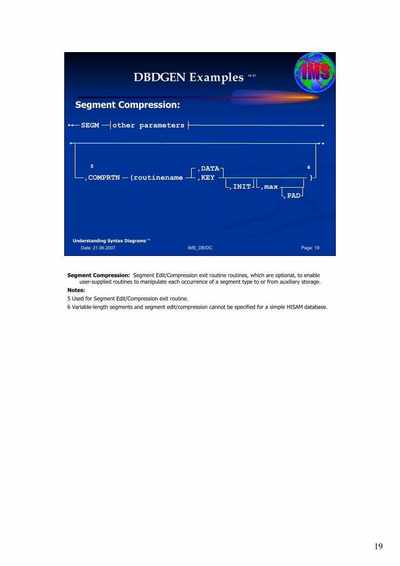
19
IMS_DB/DC Page: 19Date: 21.06.2007
DBDGEN Examples (6-2)
Segment Compression:
,DATA
,COMPRTN (routinename ,KEY )
,INIT ,max
,PAD
SEGM other parameters
5 6
Understanding Syntax Diagrams (2)
Segment Compression: Segment Edit/Compression exit routine routines, which are optional, to enable user-supplied routines to manipulate each occurrence of a segment type to or from auxiliary storage.
Notes:
5 Used for Segment Edit/Compression exit routine.
6 Variable-length segments and segment edit/compression cannot be specified for a simple HISAM database.
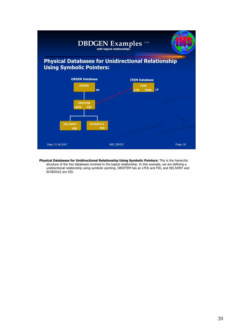
20
IMS_DB/DC Page: 20Date: 21.06.2007
DBDGEN Examples (7-1)
with logical relationships
Physical Databases for Unidirectional Relationship Using Symbolic Pointers:
ORDER
ORDITEM
DELIVERY SCHEDULE
ORDER Database
PP
VID VID
LPCK FID
ITEM
LPCTR ITEM
ITEM Database
Physical Databases for Unidirectional Relationship Using Symbolic Pointers: This is the hierarchic structure of the two databases involved in the logical relationship. In this example, we are defining a unidirectional relationship using symbolic pointing. ORDITEM has an LPCK and FID, and DELIVERY and SCHEDULE are VID.
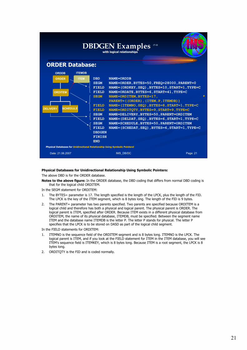
21
IMS_DB/DC Page: 21Date: 21.06.2007
DBDGEN Examples (7-2)
with logical relationships
ORDER Database:
DBD NAME=ORDDB
SEGM NAME=ORDER,BYTES=50,FREQ=28000,PARENT=0
FIELD NAME=(ORDKEY,SEQ),BYTES=10,START=1,TYPE=C
FIELD NAME=ORDATE,BYTES=6,START=41,TYPE=C
SEGM NAME=ORDITEM,BYTES=17, *
PARENT=((ORDER),(ITEM,P,ITEMDB))
FIELD NAME=(ITEMNO,SEQ),BYTES=8,START=1,TYPE=C
FIELD NAME=ORDITQTY,BYTES=9,START=9,TYPE=C
SEGM NAME=DELIVERY,BYTES=50,PARENT=ORDITEM
FIELD NAME=(DELDAT,SEQ),BYTES=6,START=1,TYPE=C
SEGM NAME=SCHEDULE,BYTES=50,PARENT=ORDITEM
FIELD NAME=(SCHEDAT,SEQ),BYTES=6,START=1,TYPE=C
DBDGEN
FINISH
END
Physical Databases for Unidirectional Relationship Using Symbolic Pointers!
ORDER
ORDITEM
DELIVERY SCHEDULE
ITEM
ORDDB ITEMDB
Physical Databases for Unidirectional Relationship Using Symbolic Pointers:
The above DBD is for the ORDER database.
Notes to the above figure: In the ORDER database, the DBD coding that differs from normal DBD coding is that for the logical child ORDITEM.
In the SEGM statement for ORDITEM:
1. The BYTES= parameter is 17. The length specified is the length of the LPCK, plus the length of the FID. The LPCK is the key of the ITEM segment, which is 8 bytes long. The length of the FID is 9 bytes.
2. The PARENT= parameter has two parents specified. Two parents are specified because ORDITEM is a logical child and therefore has both a physical and logical parent. The physical parent is ORDER. The logical parent is ITEM, specified after ORDER. Because ITEM exists in a different physical database from ORDITEM, the name of its physical database, ITEMDB, must be specified. Between the segment name ITEM and the database name ITEMDB is the letter P. The letter P stands for physical. The letter P specifies that the LPCK is to be stored on DASD as part of the logical child segment.
In the FIELD statements for ORDITEM:
1. ITEMNO is the sequence field of the ORDITEM segment and is 8 bytes long. ITEMNO is the LPCK. The logical parent is ITEM, and if you look at the FIELD statement for ITEM in the ITEM database, you will see ITEM’s sequence field is ITEMKEY, which is 8 bytes long. Because ITEM is a root segment, the LPCK is 8 bytes long.
2. ORDITQTY is the FID and is coded normally.
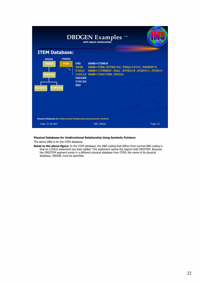
22
IMS_DB/DC Page: 22Date: 21.06.2007
DBDGEN Examples (7-3)
with logical relationships
ITEM Database:
DBD NAME=ITEMDB
SEGM NAME=ITEM,BYTES=60,FREQ=50000,PARENT=0
FIELD NAME=(ITEMKEY,SEQ),BYTES=8,START=1,TYPE=C
LCHILD NAME=(ORDITEM,ORDDB)
DBDGEN
FINISH
END
Physical Databases for Unidirectional Relationship Using Symbolic Pointers!
ORDER
ORDITEM
DELIVERY SCHEDULE
ITEM
ORDDB ITEMDB
Physical Databases for Unidirectional Relationship Using Symbolic Pointers:
The above DBD is for the ITEM database.
Notes to the above figure: In the ITEM database, the DBD coding that differs from normal DBD coding is that an LCHILD statement has been added. This statement names the logical child ORDITEM. Because the ORDITEM segment exists in a different physical database from ITEM, the name of its physical database, ORDDB, must be specified.
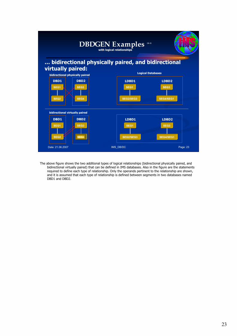
23
IMS_DB/DC Page: 23Date: 21.06.2007
DBDGEN Examples (8-1)
with logical relationships
… bidirectional physically paired, and bidirectional virtually paired:
SEG1
DBD1
SEG2
SEG3
DBD2
SEG4
bidirectional physically paired
SEG1
DBD1
SEG2
SEG3
DBD2
SEG4
bidirectional virtually paired
SEG1
LDBD1
SEG2/SEG3
SEG3
LDBD2
SEG4/SEG1
Logical Databases
SEG1
LDBD1
SEG2/SEG3
SEG3
LDBD2
SEG4/SEG1
The above figure shows the two additional types of logical relationships (bidirectional physically paired, and bidirectional virtually paired) that can be defined in IMS databases. Also in the figure are the statements required to define each type of relationship. Only the operands pertinent to the relationship are shown, and it is assumed that each type of relationship is defined between segments in two databases named DBD1 and DBD2.
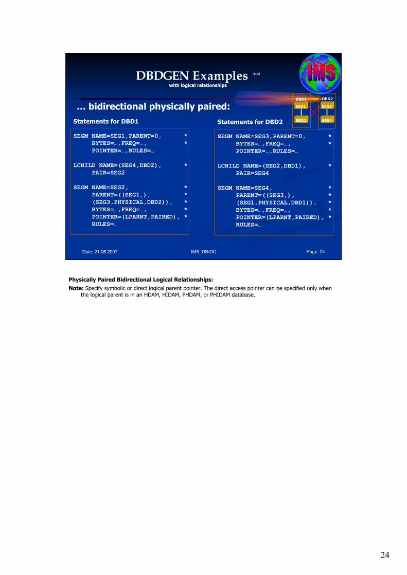
24
IMS_DB/DC Page: 24Date: 21.06.2007
DBDGEN Examples (8-2)
with logical relationships
… bidirectional physically paired:
Statements for DBD1
SEGM NAME=SEG1,PARENT=0, *
BYTES=…,FREQ=…, *
POINTER=…,RULES=…
LCHILD NAME=(SEG4,DBD2), *
PAIR=SEG2
SEGM NAME=SEG2, *
PARENT=((SEG1,), *
(SEG3,PHYSICAL,DBD2)), *
BYTES=…,FREQ=…, *
POINTER=(LPARNT,PAIRED), *
RULES=…
SEG1
DBD1
SEG2
SEG3
DBD2
SEG4Statements for DBD2
SEGM NAME=SEG3,PARENT=0, *
BYTES=…,FREQ=…, *
POINTER=…,RULES=…
LCHILD NAME=(SEG2,DBD1), *
PAIR=SEG4
SEGM NAME=SEG4, *
PARENT=((SEG3,), *
(SEG1,PHYSICAL,DBD1)), *
BYTES=…,FREQ=…, *
POINTER=(LPARNT,PAIRED), *
RULES=…
Physically Paired Bidirectional Logical Relationships:
Note: Specify symbolic or direct logical parent pointer. The direct access pointer can be specified only when the logical parent is in an HDAM, HIDAM, PHDAM, or PHIDAM database.
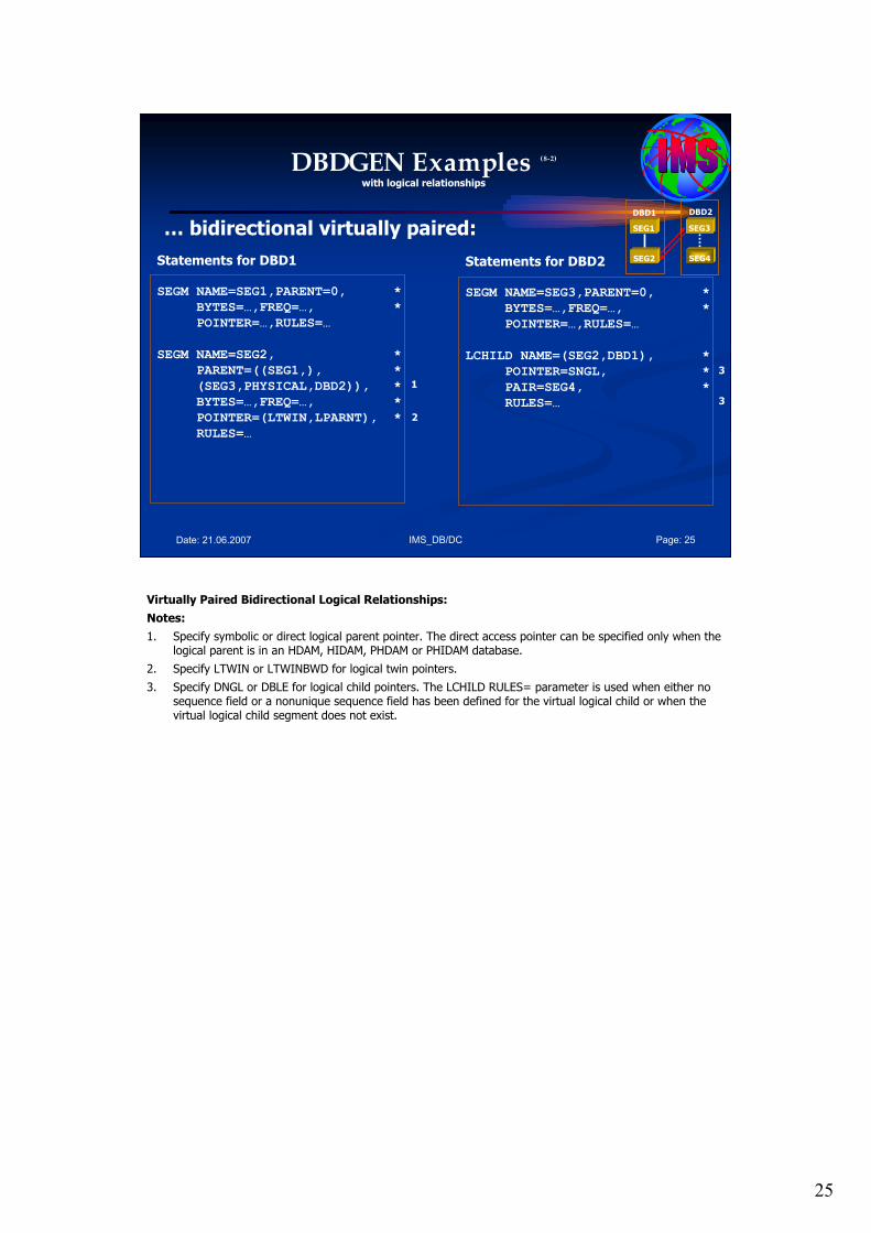
25
IMS_DB/DC Page: 25Date: 21.06.2007
DBDGEN Examples (8-2)
with logical relationships
… bidirectional virtually paired: SEG1
DBD1
SEG2
SEG3
DBD2
SEG4Statements for DBD1
SEGM NAME=SEG1,PARENT=0, *
BYTES=…,FREQ=…, *
POINTER=…,RULES=…
SEGM NAME=SEG2, *
PARENT=((SEG1,), *
(SEG3,PHYSICAL,DBD2)), *
BYTES=…,FREQ=…, *
POINTER=(LTWIN,LPARNT), *
RULES=…
1
2
Statements for DBD2
SEGM NAME=SEG3,PARENT=0, *
BYTES=…,FREQ=…, *
POINTER=…,RULES=…
LCHILD NAME=(SEG2,DBD1), *
POINTER=SNGL, *
PAIR=SEG4, *
RULES=…
3
3
Virtually Paired Bidirectional Logical Relationships:
Notes:
1. Specify symbolic or direct logical parent pointer. The direct access pointer can be specified only when the logical parent is in an HDAM, HIDAM, PHDAM or PHIDAM database.
2. Specify LTWIN or LTWINBWD for logical twin pointers.
3. Specify DNGL or DBLE for logical child pointers. The LCHILD RULES= parameter is used when either no sequence field or a nonunique sequence field has been defined for the virtual logical child or when the virtual logical child segment does not exist.
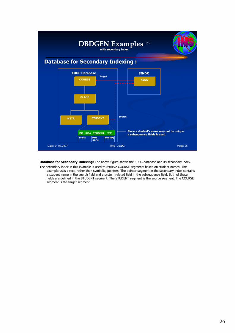
26
IMS_DB/DC Page: 26Date: 21.06.2007
DBDGEN Examples (9-1)
with secondary index
Database for Secondary Indexing :
COURSE
CLASS
INSTR STUDENT
EDUC Database
XSEG
SINDX
DB RBA STUDNM /SX1
Prefix Data SUBSEQSRCH
Since a student’s name may not be unique,a subsequence fields is used.
Source
Target
Database for Secondary Indexing: The above figure shows the EDUC database and its secondary index.
The secondary index in this example is used to retrieve COURSE segments based on student names. The example uses direct, rather than symbolic, pointers. The pointer segment in the secondary index contains a student name in the search field and a system related field in the subsequence field. Both of these fields are defined in the STUDENT segment. The STUDENT segment is the source segment. The COURSE segment is the target segment.
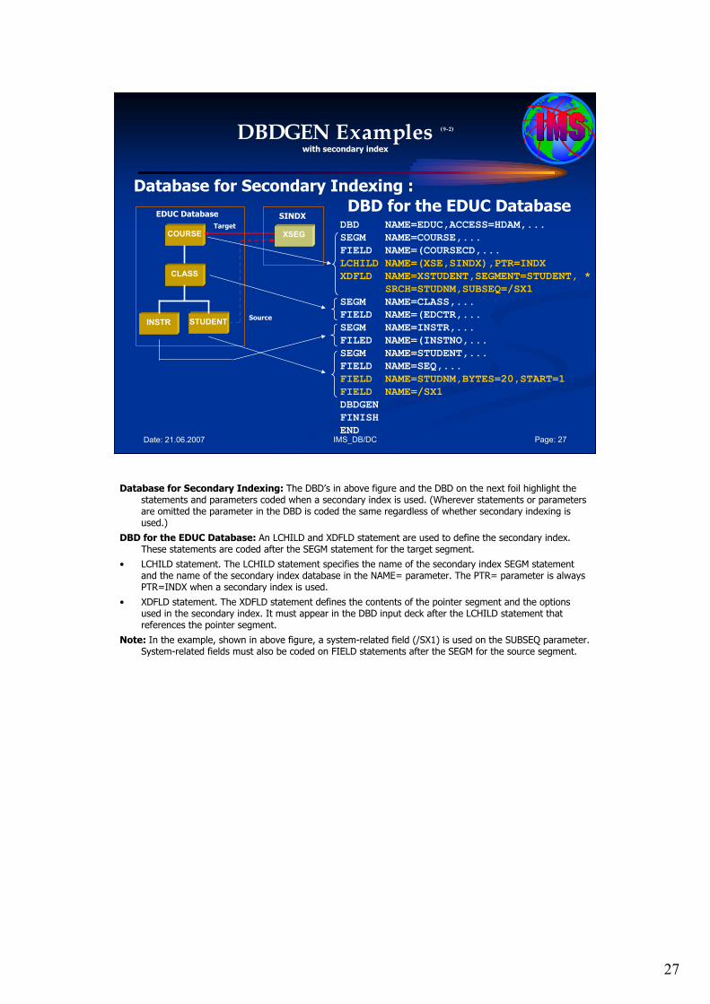
27
IMS_DB/DC Page: 27Date: 21.06.2007
DBDGEN Examples (9-2)
with secondary index
Database for Secondary Indexing :
COURSE
CLASS
INSTR STUDENT
EDUC Database
XSEG
SINDX
Source
Target DBD NAME=EDUC,ACCESS=HDAM,...
SEGM NAME=COURSE,...
FIELD NAME=(COURSECD,...
LCHILD NAME=(XSE,SINDX),PTR=INDX
XDFLD NAME=XSTUDENT,SEGMENT=STUDENT, *
SRCH=STUDNM,SUBSEQ=/SX1
SEGM NAME=CLASS,...
FIELD NAME=(EDCTR,...
SEGM NAME=INSTR,...
FILED NAME=(INSTNO,...
SEGM NAME=STUDENT,...
FIELD NAME=SEQ,...
FIELD NAME=STUDNM,BYTES=20,START=1
FIELD NAME=/SX1
DBDGEN
FINISH
END
DBD for the EDUC Database
Database for Secondary Indexing: The DBD’s in above figure and the DBD on the next foil highlight the statements and parameters coded when a secondary index is used. (Wherever statements or parameters are omitted the parameter in the DBD is coded the same regardless of whether secondary indexing is used.)
DBD for the EDUC Database: An LCHILD and XDFLD statement are used to define the secondary index. These statements are coded after the SEGM statement for the target segment.
• LCHILD statement. The LCHILD statement specifies the name of the secondary index SEGM statement and the name of the secondary index database in the NAME= parameter. The PTR= parameter is always PTR=INDX when a secondary index is used.
• XDFLD statement. The XDFLD statement defines the contents of the pointer segment and the options used in the secondary index. It must appear in the DBD input deck after the LCHILD statement that references the pointer segment.
Note: In the example, shown in above figure, a system-related field (/SX1) is used on the SUBSEQ parameter. System-related fields must also be coded on FIELD statements after the SEGM for the source segment.
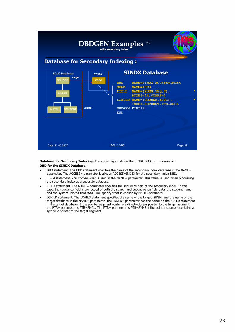
28
IMS_DB/DC Page: 28Date: 21.06.2007
DBDGEN Examples (9-3)
with secondary index
Database for Secondary Indexing :
COURSE
CLASS
INSTR STUDENT
EDUC Database
XSEG
SINDX
Source
Target
SINDX Database
DBD NAME=SINDX,ACCESS=INDEX
SEGM NAME=XSEG,...
FIELD NAME=(XSEG,SEQ,U), *
BYTES=24,START=1
LCHILD NAME=(COURSE,EDUC), *
INDEX=XSTUDNT,PTR=SNGL
DBDGEN FINISH
END
Database for Secondary Indexing: The above figure shows the SINDX DBD for the example.
DBD for the SINDX Database:
• DBD statement. The DBD statement specifies the name of the secondary index database in the NAME= parameter. The ACCESS= parameter is always ACCESS=INDEX for the secondary index DBD.
• SEGM statement. You choose what is used in the NAME= parameter. This value is used when processing the secondary index as a separate database.
• FIELD statement. The NAME= parameter specifies the sequence field of the secondary index. In this case, the sequence field is composed of both the search and subsequence field data, the student name, and the system-related field /SX1. You specify what is chosen by NAME=parameter.
• LCHILD statement. The LCHILD statement specifies the name of the target, SEGM, and the name of the target database in the NAME= parameter. The INDEX= parameter has the name on the XDFLD statement in the target database. If the pointer segment contains a direct-address pointer to the target segment, the PTR= parameter is PTR=SNGL. The PTR= parameter is PTR=SYMB if the pointer segment contains a symbolic pointer to the target segment.
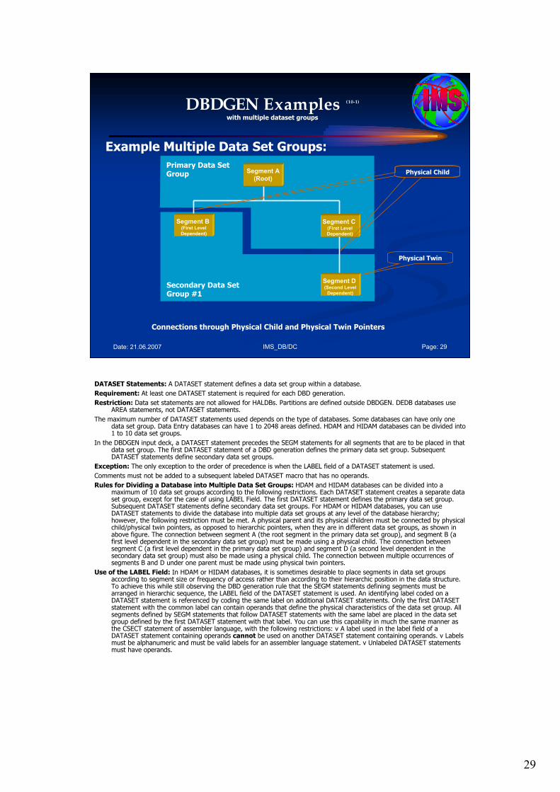
29
IMS_DB/DC Page: 29Date: 21.06.2007
DBDGEN Examples (10-1)
with multiple dataset groups
Example Multiple Data Set Groups:
Connections through Physical Child and Physical Twin Pointers
Segment A
(Root)
Segment B (First Level
Dependent)
Segment C (First Level
Dependent)
Segment D (Second Level
Dependent)
Primary Data SetGroup
Secondary Data SetGroup #1
Physical Child
Physical Twin
DATASET Statements: A DATASET statement defines a data set group within a database.
Requirement: At least one DATASET statement is required for each DBD generation.
Restriction: Data set statements are not allowed for HALDBs. Partitions are defined outside DBDGEN. DEDB databases use AREA statements, not DATASET statements.
The maximum number of DATASET statements used depends on the type of databases. Some databases can have only one data set group. Data Entry databases can have 1 to 2048 areas defined. HDAM and HIDAM databases can be divided into 1 to 10 data set groups.
In the DBDGEN input deck, a DATASET statement precedes the SEGM statements for all segments that are to be placed in that data set group. The first DATASET statement of a DBD generation defines the primary data set group. Subsequent DATASET statements define secondary data set groups.
Exception: The only exception to the order of precedence is when the LABEL field of a DATASET statement is used.
Comments must not be added to a subsequent labeled DATASET macro that has no operands.
Rules for Dividing a Database into Multiple Data Set Groups: HDAM and HIDAM databases can be divided into a maximum of 10 data set groups according to the following restrictions. Each DATASET statement creates a separate data set group, except for the case of using LABEL Field. The first DATASET statement defines the primary data set group. Subsequent DATASET statements define secondary data set groups. For HDAM or HIDAM databases, you can use DATASET statements to divide the database into multiple data set groups at any level of the database hierarchy; however, the following restriction must be met. A physical parent and its physical children must be connected by physical child/physical twin pointers, as opposed to hierarchic pointers, when they are in different data set groups, as shown in above figure. The connection between segment A (the root segment in the primary data set group), and segment B (a first level dependent in the secondary data set group) must be made using a physical child. The connection between segment C (a first level dependent in the primary data set group) and segment D (a second level dependent in the secondary data set group) must also be made using a physical child. The connection between multiple occurrences of segments B and D under one parent must be made using physical twin pointers.
Use of the LABEL Field: In HDAM or HIDAM databases, it is sometimes desirable to place segments in data set groups according to segment size or frequency of access rather than according to their hierarchic position in the data structure. To achieve this while still observing the DBD generation rule that the SEGM statements defining segments must be arranged in hierarchic sequence, the LABEL field of the DATASET statement is used. An identifying label coded on a DATASET statement is referenced by coding the same label on additional DATASET statements. Only the first DATASET statement with the common label can contain operands that define the physical characteristics of the data set group. All segments defined by SEGM statements that follow DATASET statements with the same label are placed in the data set group defined by the first DATASET statement with that label. You can use this capability in much the same manner as the CSECT statement of assembler language, with the following restrictions: v A label used in the label field of a DATASET statement containing operands cannot be used on another DATASET statement containing operands. v Labels must be alphanumeric and must be valid labels for an assembler language statement. v Unlabeled DATASET statements must have operands.
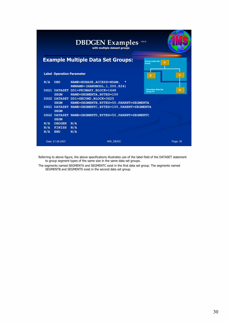
30
IMS_DB/DC Page: 30Date: 21.06.2007
DBDGEN Examples (10-2)
with multiple dataset groups
Example Multiple Data Set Groups:
Label Operation Parameter
N/A DBD NAME=HDBASE,ACCESS=HDAM, *
RMNAME=(RANDMODL,1,500,824)
DSG1 DATASET DD1=PRIMARY,BLOCK=1648
SEGM NAME=SEGMENTA,BYTES=100
DSG2 DATASET DD1=SECOND,BLOCK=3625
SEGM NAME=SEGMENTB,BYTES=50,PARENT=SEGMENTA
DSG1 DATASET NAME=SEGMENTC,BYTES=100,PARENT=SEGMENTA
SEGM
DSG2 DATASET NAME=SEGMENTD,BYTES=50,PARENT=SEGMENTC
SEGM
N/A DBDGEN N/A
N/A FINISH N/A
N/A END N/A
A
B C
D
Primary Data SetGroup
Secondary Data SetGroup #1
Referring to above figure, the above specifications illustrates use of the label field of the DATASET statement to group segment types of the same size in the same data set groups.
The segments named SEGMENTA and SEGMENTC exist in the first data set group. The segments named SEGMENTB and SEGMENTD exist in the second data set group.
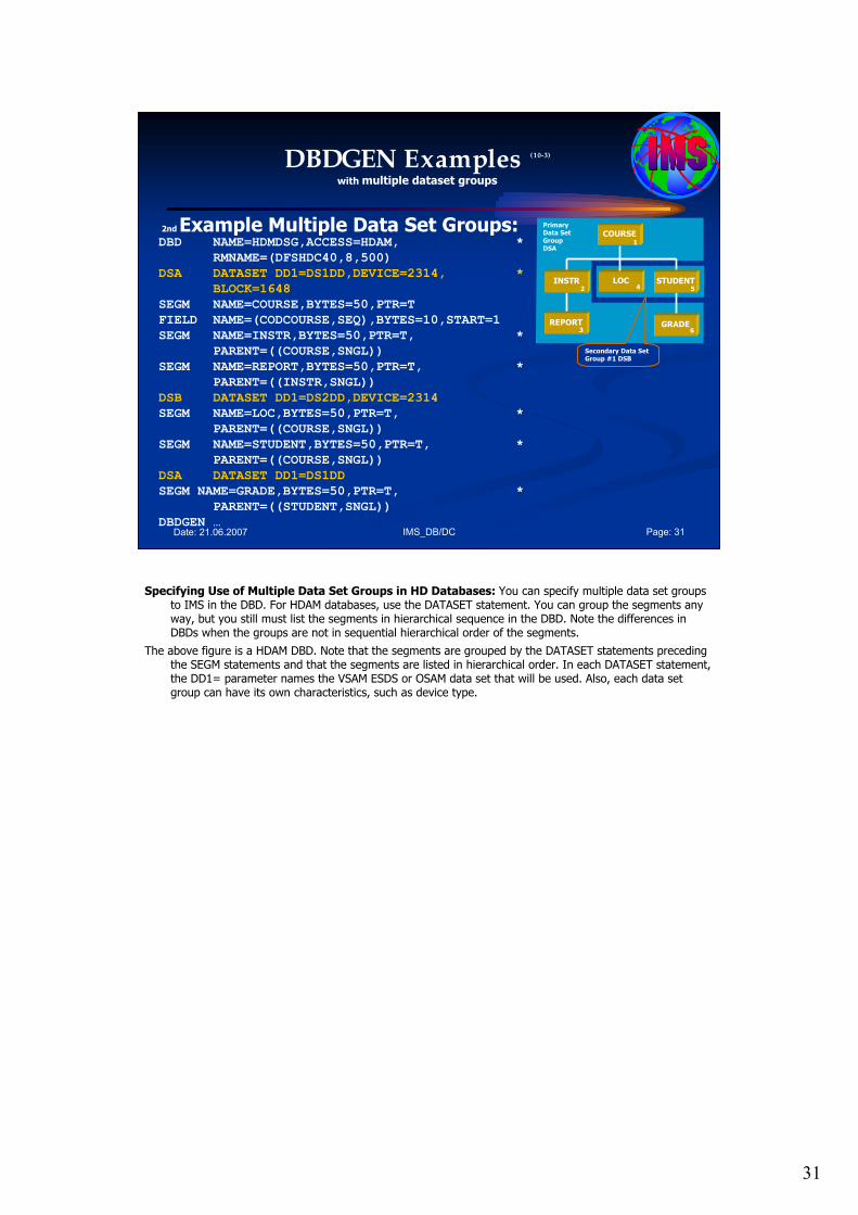
31
IMS_DB/DC Page: 31Date: 21.06.2007
DBDGEN Examples (10-3)
with multiple dataset groups
2nd Example Multiple Data Set Groups:COURSE
Primary Data SetGroupDSA
Secondary Data SetGroup #1 DSB
STUDENT
REPORT GRADE
INSTR LOC
1
2
3
4 5
6
DBD NAME=HDMDSG,ACCESS=HDAM, *
RMNAME=(DFSHDC40,8,500)
DSA DATASET DD1=DS1DD,DEVICE=2314, *
BLOCK=1648
SEGM NAME=COURSE,BYTES=50,PTR=T
FIELD NAME=(CODCOURSE,SEQ),BYTES=10,START=1
SEGM NAME=INSTR,BYTES=50,PTR=T, *
PARENT=((COURSE,SNGL))
SEGM NAME=REPORT,BYTES=50,PTR=T, *
PARENT=((INSTR,SNGL))
DSB DATASET DD1=DS2DD,DEVICE=2314
SEGM NAME=LOC,BYTES=50,PTR=T, *
PARENT=((COURSE,SNGL))
SEGM NAME=STUDENT,BYTES=50,PTR=T, *
PARENT=((COURSE,SNGL))
DSA DATASET DD1=DS1DD
SEGM NAME=GRADE,BYTES=50,PTR=T, *
PARENT=((STUDENT,SNGL))
DBDGEN …
Specifying Use of Multiple Data Set Groups in HD Databases: You can specify multiple data set groups to IMS in the DBD. For HDAM databases, use the DATASET statement. You can group the segments any way, but you still must list the segments in hierarchical sequence in the DBD. Note the differences in DBDs when the groups are not in sequential hierarchical order of the segments.
The above figure is a HDAM DBD. Note that the segments are grouped by the DATASET statements preceding the SEGM statements and that the segments are listed in hierarchical order. In each DATASET statement, the DD1= parameter names the VSAM ESDS or OSAM data set that will be used. Also, each data set group can have its own characteristics, such as device type.

32
IMS_DB/DC Page: 32Date: 21.06.2007
Agenda
Session 7: Implementing IMS Databases
1. Basic Terms
2. DBDGEN
• Physical DB’s
• Logical DB’s
3. PSBGEN
4. ACBGEN
Logical DB’s
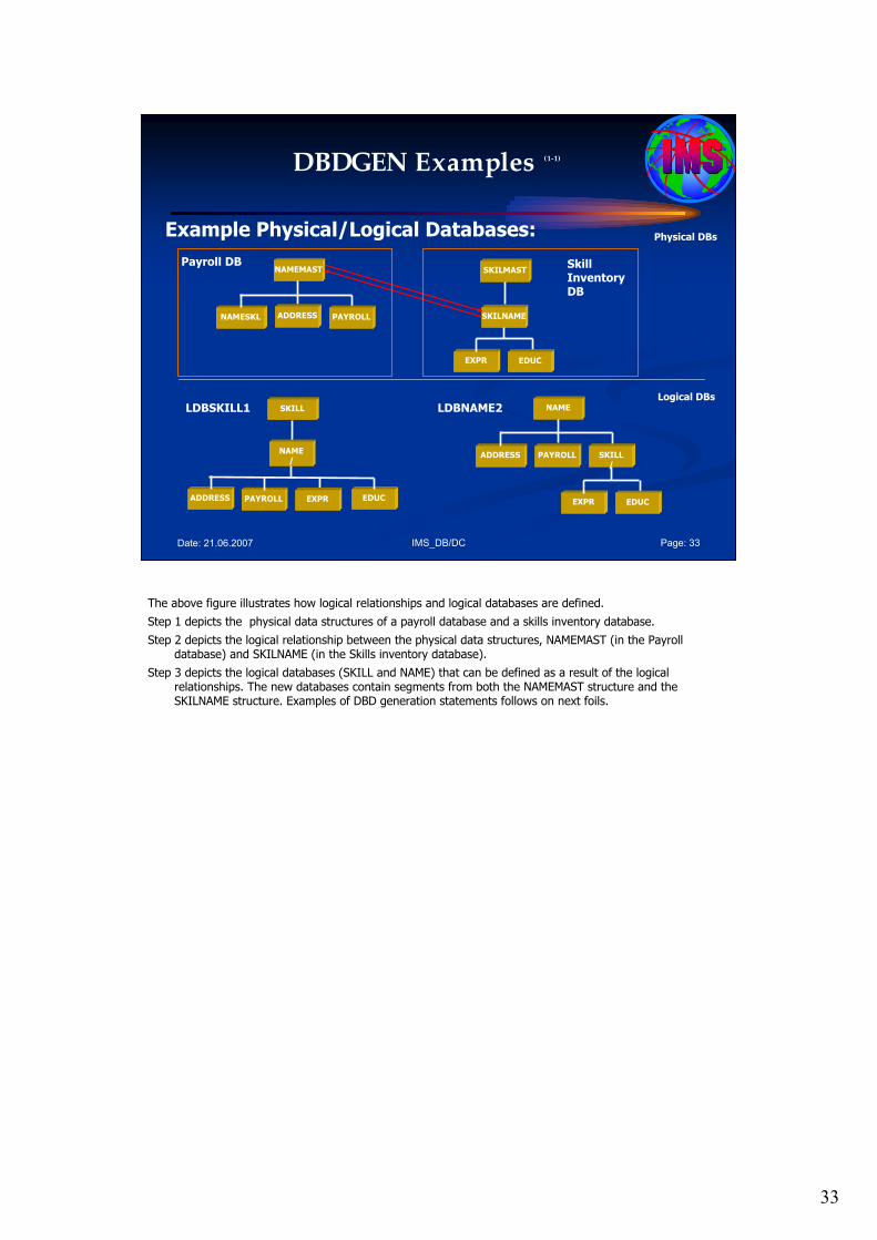
33
IMS_DB/DC Page: 33Date: 21.06.2007
DBDGEN Examples (1-1)
Example Physical/Logical Databases:
NAMEMAST
PAYROLLNAMESKL ADDRESS
SKILMAST
SKILNAME
EDUCEXPR
Payroll DB Skill Inventory DB
Physical DBs
SKILL
NAME/
EXPRPAYROLLADDRESS EDUC
NAME
SKILL/
ADDRESS PAYROLL
EDUCEXPR
LDBSKILL1 LDBNAME2Logical DBs
The above figure illustrates how logical relationships and logical databases are defined.
Step 1 depicts the physical data structures of a payroll database and a skills inventory database.
Step 2 depicts the logical relationship between the physical data structures, NAMEMAST (in the Payroll database) and SKILNAME (in the Skills inventory database).
Step 3 depicts the logical databases (SKILL and NAME) that can be defined as a result of the logical relationships. The new databases contain segments from both the NAMEMAST structure and the SKILNAME structure. Examples of DBD generation statements follows on next foils.
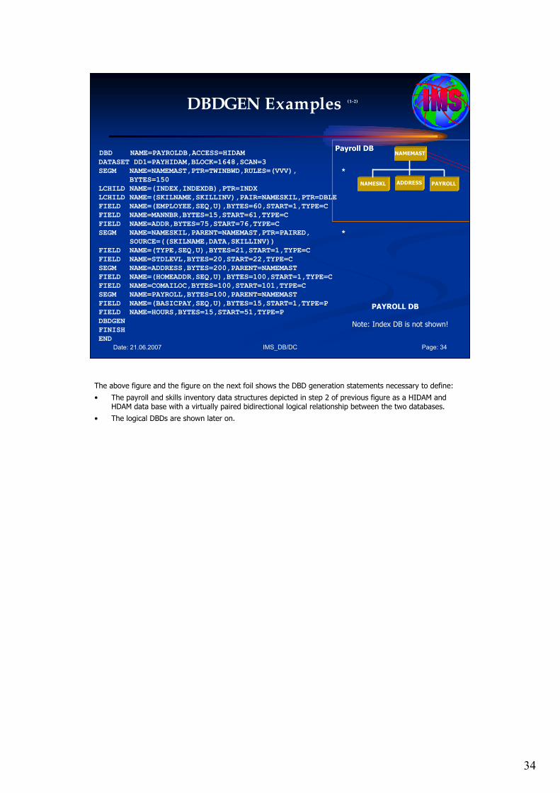
34
IMS_DB/DC Page: 34Date: 21.06.2007
DBDGEN Examples (1-2)
DBD NAME=PAYROLDB,ACCESS=HIDAM
DATASET DD1=PAYHIDAM,BLOCK=1648,SCAN=3
SEGM NAME=NAMEMAST,PTR=TWINBWD,RULES=(VVV), *
BYTES=150
LCHILD NAME=(INDEX,INDEXDB),PTR=INDX
LCHILD NAME=(SKILNAME,SKILLINV),PAIR=NAMESKIL,PTR=DBLE
FIELD NAME=(EMPLOYEE,SEQ,U),BYTES=60,START=1,TYPE=C
FIELD NAME=MANNBR,BYTES=15,START=61,TYPE=C
FIELD NAME=ADDR,BYTES=75,START=76,TYPE=C
SEGM NAME=NAMESKIL,PARENT=NAMEMAST,PTR=PAIRED, *
SOURCE=((SKILNAME,DATA,SKILLINV))
FIELD NAME=(TYPE,SEQ,U),BYTES=21,START=1,TYPE=C
FIELD NAME=STDLEVL,BYTES=20,START=22,TYPE=C
SEGM NAME=ADDRESS,BYTES=200,PARENT=NAMEMAST
FIELD NAME=(HOMEADDR,SEQ,U),BYTES=100,START=1,TYPE=C
FIELD NAME=COMAILOC,BYTES=100,START=101,TYPE=C
SEGM NAME=PAYROLL,BYTES=100,PARENT=NAMEMAST
FIELD NAME=(BASICPAY,SEQ,U),BYTES=15,START=1,TYPE=P
FIELD NAME=HOURS,BYTES=15,START=51,TYPE=P
DBDGEN
FINISH
END
PAYROLL DB
Note: Index DB is not shown!
NAMEMAST
PAYROLLNAMESKL ADDRESS
Payroll DB
The above figure and the figure on the next foil shows the DBD generation statements necessary to define:
• The payroll and skills inventory data structures depicted in step 2 of previous figure as a HIDAM and HDAM data base with a virtually paired bidirectional logical relationship between the two databases.
• The logical DBDs are shown later on.
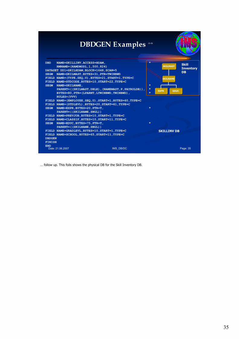
35
IMS_DB/DC Page: 35Date: 21.06.2007
DBDGEN Examples (1-3)
DBD NAME=SKILLINV,ACCESS=HDAM, *
RMNAME=(RAMDMODL,1,500,824)
DATASET DD1=SKILHDAM,BLOCK=1648,SCAN=5
SEGM NAME=SKILMAST,BYTES=31,PTR=TWINBWD
FIELD NAME=(TYPE,SEQ,U),BYTES=21,START=1,TYPE=C
FIELD NAME=STDCODE,BYTES=10,START=22,TYPE=C
SEGM NAME=SKILNAME, *
PARENT=((SKILMAST,DBLE),(NAMEMAST,P,PAYROLDB)), *
BYTES=80,PTR=(LPARNT,LTWINBWD,TWINBWD), *
RULES=(VVV)
FIELD NAME=(EMPLOYEE,SEQ,U),START=1,BYTES=60,TYPE=C
FIELD NAME=(STDLEVL),BYTES=20,START=61,TYPE=C
SEGM NAME=EXPR,BYTES=20,PTR=T, *
PARENT=((SKILNAME,SNGL))
FIELD NAME=PREVJOB,BYTES=10,START=1,TYPE=C
FIELD NAME=CLASSIF,BYTES=10,START=11,TYPE=C
SEGM NAME=EDUC,BYTES=75,PTR=T, *
PARENT=((SKILNAME,SNGL))
FIELD NAME=GRADLEVL,BYTES=10,START=1,TYPE=C
FIELD NAME=SCHOOL,BYTES=65,START=11,TYPE=C
DBDGEN
FINISH
END
SKILLINV DB
SKILMAST
SKILNAME
EDUCEXPR
Skill Inventory DB
… follow up. This foils shows the physical DB for the Skill Inventory DB.
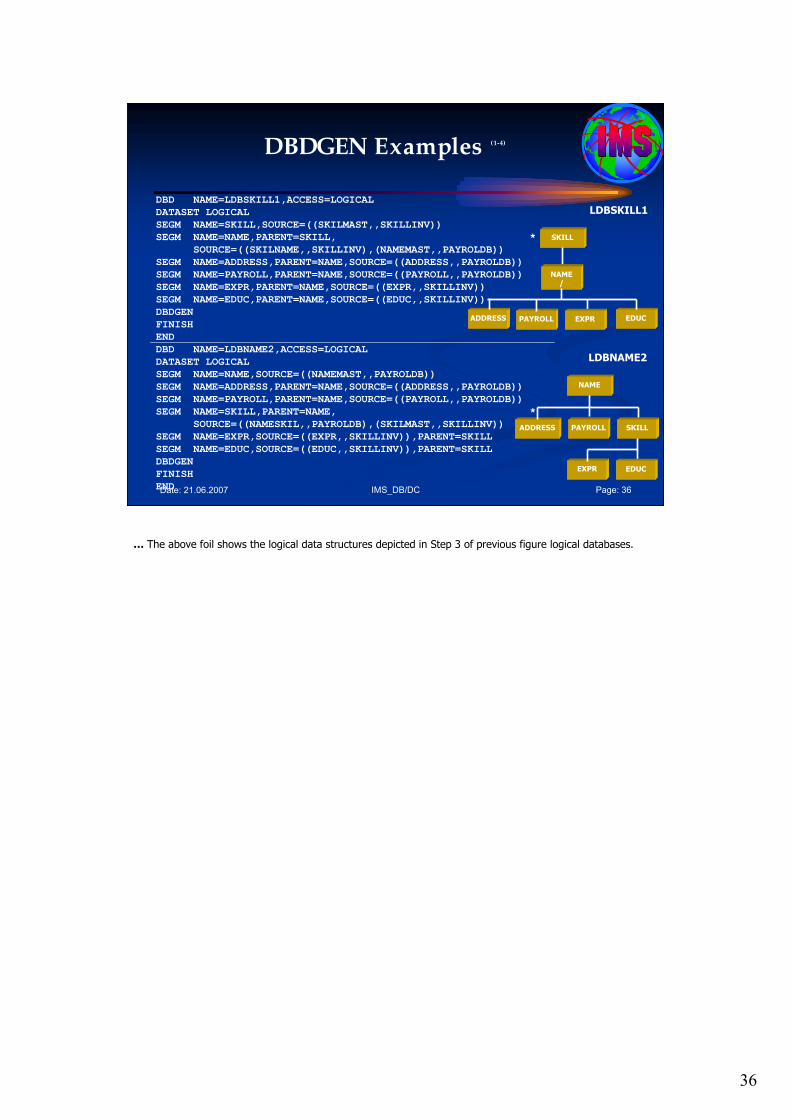
36
IMS_DB/DC Page: 36Date: 21.06.2007
DBDGEN Examples (1-4)
DBD NAME=LDBSKILL1,ACCESS=LOGICAL
DATASET LOGICAL
SEGM NAME=SKILL,SOURCE=((SKILMAST,,SKILLINV))
SEGM NAME=NAME,PARENT=SKILL, *
SOURCE=((SKILNAME,,SKILLINV),(NAMEMAST,,PAYROLDB))
SEGM NAME=ADDRESS,PARENT=NAME,SOURCE=((ADDRESS,,PAYROLDB))
SEGM NAME=PAYROLL,PARENT=NAME,SOURCE=((PAYROLL,,PAYROLDB))
SEGM NAME=EXPR,PARENT=NAME,SOURCE=((EXPR,,SKILLINV))
SEGM NAME=EDUC,PARENT=NAME,SOURCE=((EDUC,,SKILLINV))
DBDGEN
FINISH
END
DBD NAME=LDBNAME2,ACCESS=LOGICAL
DATASET LOGICAL
SEGM NAME=NAME,SOURCE=((NAMEMAST,,PAYROLDB))
SEGM NAME=ADDRESS,PARENT=NAME,SOURCE=((ADDRESS,,PAYROLDB))
SEGM NAME=PAYROLL,PARENT=NAME,SOURCE=((PAYROLL,,PAYROLDB))
SEGM NAME=SKILL,PARENT=NAME, *
SOURCE=((NAMESKIL,,PAYROLDB),(SKILMAST,,SKILLINV))
SEGM NAME=EXPR,SOURCE=((EXPR,,SKILLINV)),PARENT=SKILL
SEGM NAME=EDUC,SOURCE=((EDUC,,SKILLINV)),PARENT=SKILL
DBDGEN
FINISH
END
SKILL
NAME/
EXPRPAYROLLADDRESS EDUC
LDBSKILL1
NAME
SKILLADDRESS PAYROLL
EDUCEXPR
LDBNAME2
… The above foil shows the logical data structures depicted in Step 3 of previous figure logical databases.
37
IMS_DB/DC Page: 37Date: 21.06.2007
Agenda
Session 7: Implementing IMS Databases
1. Basic Terms
2. DBDGEN
• Physical DB’s
• Logical DB’s
3. PSBGEN
4. ACBGEN
3. PSBGEN
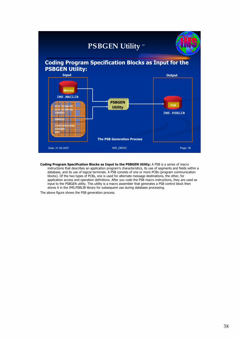
38
IMS_DB/DC Page: 38Date: 21.06.2007
PSBGEN Utility (1)
Coding Program Specification Blocks as Input for the PSBGEN Utility:
Macros
IMS.MACLIB
IMS.PSBLIB
PCB TYPE=TP
PCB TYPE=DB
SENSEG
…
SENFLD
…
PCBTYPE=GSAM
PSBGEN
END
PSBPSBGEN
Utility
The PSB Generation Process
Input Output
Coding Program Specification Blocks as Input to the PSBGEN Utility: A PSB is a series of macro instructions that describes an application program’s characteristics, its use of segments and fields within a database, and its use of logical terminals. A PSB consists of one or more PCBs (program communication blocks). Of the two types of PCBs, one is used for alternate message destinations, the other, for application access and operation definitions. After you code the PSB macro instructions, they are used as input to the PSBGEN utility. This utility is a macro assembler that generates a PSB control block then stores it in the IMS.PSBLIB library for subsequent use during database processing.
The above figure shows the PSB generation process.
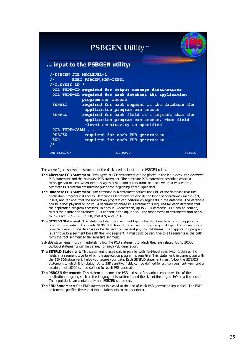
39
IMS_DB/DC Page: 39Date: 21.06.2007
PSBGEN Utility (2)
… input to the PSBGEN utility:
//PSBGEN JOB MSGLEVEL=1
// EXEC PSBGEN,MBR=PSBT1
//C.SYSIN DD *
PCB TYPE=TP required for output message destinations
PCB TYPE=DB required for each database the application
program can access
SENSEG required for each segment in the database the
application program can access
SENFLD required for each field in a segment that the
application program can access, when field
-level sensitivity is specified
PCB TYPE=GSAM ...
PSBGEN required for each PSB generation
END required for each PSB generation
/*
The above figure shows the structure of the deck used as input to the PSBGEN utility.
The Alternate PCB Statement: Two types of PCB statements can be placed in the input deck: the alternate PCB statement and the database PCB statement. The alternate PCB statement describes where a message can be sent when the message’s destination differs from the place where it was entered. Alternate PCB statements must be put at the beginning of the input deck.
The Database PCB Statement: The database PCB statement defines the DBD of the database that the application program will access. Database PCB statements also define types of operations (such as get, insert, and replace) that the application program can perform on segments in the database. The database can be either physical or logical. A separate database PCB statement is required for each database that the application program accesses. In each PSB generation, up to 2500 database PCBs can be defined, minus the number of alternate PCBs defined in the input deck. The other forms of statements that apply to PSBs are SENSEG, SENFLD, PSBGEN, and END.
The SENSEG Statement: This statement defines a segment type in the database to which the application program is sensitive. A separate SENSEG statement must exist for each segment type. The segments can physically exist in one database or be derived from several physical databases. If an application program is sensitive to a segment beneath the root segment, it must also be sensitive to all segments in the path from the root segment to the sensitive segment.
SENSEG statements must immediately follow the PCB statement to which they are related. Up to 30000 SENSEG statements can be defined for each PSB generation.
The SENFLD Statement: This statement is used only in parallel with field-level sensitivity. It defines the fields in a segment type to which the application program is sensitive. This statement, in conjunction with the SENSEG statement, helps you secure your data. Each SENFLD statement must follow the SENSEG statement to which it is related. Up to 255 sensitive fields can be defined for a given segment type, and a maximum of 10000 can be defined for each PSB generation.
The PSBGEN Statement: This statement names the PSB and specifies various characteristics of the application program, such as the language it is written in and the size of the largest I/O area it can use. The input deck can contain only one PSBGEN statement.
The END Statement: One END statement is placed at the end of each PSB generation input deck. The END statement specifies the end of input statements to the assembler.
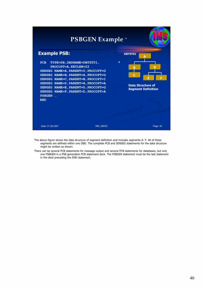
40
IMS_DB/DC Page: 40Date: 21.06.2007
PSBGEN Example (1)
PCB TYPE=DB,DBDNAME=DBTST01, *
PROCOPT=A,KEYLEN=22
SENSEG NAME=A,PARENT=0,PROCOPT=G
SENSEG NAME=B,PARENT=A,PROCOPT=G
SENSEG NAME=C,PARENT=B,PROCOPT=I
SENSEG NAME=D,PARENT=A,PROCOPT=A
SENSEG NAME=E,PARENT=D,PROCOPT=G
SENSEG NAME=F,PARENT=D,PROCOPT=A
PSBGEN …
END
A
DB
CFE
Data Structure ofSegment Definition
DBTST01Example PSB:
The above figure shows the data structure of segment definition and includes segments A- F. All of these segments are defined within one DBD. The complete PCB and SENSEG statements for the data structure might be written as shown.
There can be several PCB statements for message output and several PCB statements for databases, but only one PSBGEN in a PSB generation PCB statement deck. The PSBGEN statement must be the last statement in the deck preceding the END statement.
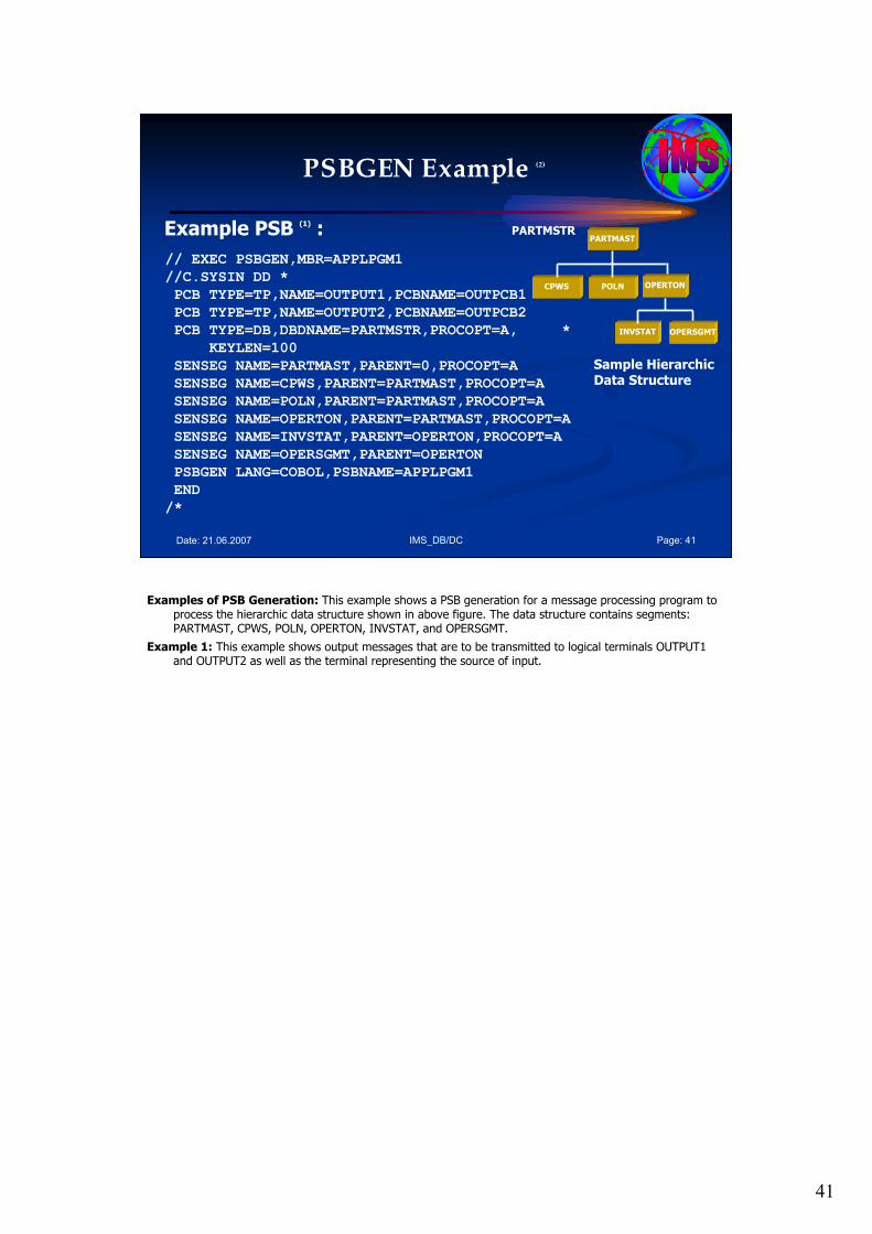
41
IMS_DB/DC Page: 41Date: 21.06.2007
PSBGEN Example (2)
PARTMAST
OPERTONCPWS POLN
OPERSGMTINVSTAT
Sample HierarchicData Structure
PARTMSTRExample PSB (1) :
// EXEC PSBGEN,MBR=APPLPGM1
//C.SYSIN DD *
PCB TYPE=TP,NAME=OUTPUT1,PCBNAME=OUTPCB1
PCB TYPE=TP,NAME=OUTPUT2,PCBNAME=OUTPCB2
PCB TYPE=DB,DBDNAME=PARTMSTR,PROCOPT=A, *
KEYLEN=100
SENSEG NAME=PARTMAST,PARENT=0,PROCOPT=A
SENSEG NAME=CPWS,PARENT=PARTMAST,PROCOPT=A
SENSEG NAME=POLN,PARENT=PARTMAST,PROCOPT=A
SENSEG NAME=OPERTON,PARENT=PARTMAST,PROCOPT=A
SENSEG NAME=INVSTAT,PARENT=OPERTON,PROCOPT=A
SENSEG NAME=OPERSGMT,PARENT=OPERTON
PSBGEN LANG=COBOL,PSBNAME=APPLPGM1
END
/*
Examples of PSB Generation: This example shows a PSB generation for a message processing program to process the hierarchic data structure shown in above figure. The data structure contains segments: PARTMAST, CPWS, POLN, OPERTON, INVSTAT, and OPERSGMT.
Example 1: This example shows output messages that are to be transmitted to logical terminals OUTPUT1 and OUTPUT2 as well as the terminal representing the source of input.
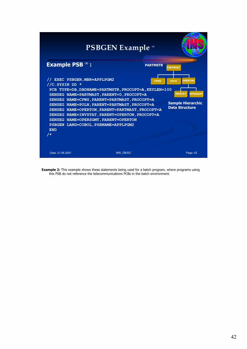
42
IMS_DB/DC Page: 42Date: 21.06.2007
PSBGEN Example (3)
PARTMAST
OPERTONCPWS POLN
OPERSGMTINVSTAT
Sample HierarchicData Structure
PARTMSTRExample PSB (2) :
// EXEC PSBGEN,MBR=APPLPGM2
//C.SYSIN DD *
PCB TYPE=DB,DBDNAME=PARTMSTR,PROCOPT=A,KEYLEN=100
SENSEG NAME=PARTMAST,PARENT=0,PROCOPT=A
SENSEG NAME=CPWS,PARENT=PARTMAST,PROCOPT=A
SENSEG NAME=POLN,PARENT=PARTMAST,PROCOPT=A
SENSEG NAME=OPERTON,PARENT=PARTMAST,PROCOPT=A
SENSEG NAME=INVSTAT,PARENT=OPERTON,PROCOPT=A
SENSEG NAME=OPERSGMT,PARENT=OPERTON
PSBGEN LANG=COBOL,PSBNAME=APPLPGM2
END
/*
Example 2: This example shows these statements being used for a batch program, where programs using this PSB do not reference the telecommunications PCBs in the batch environment.
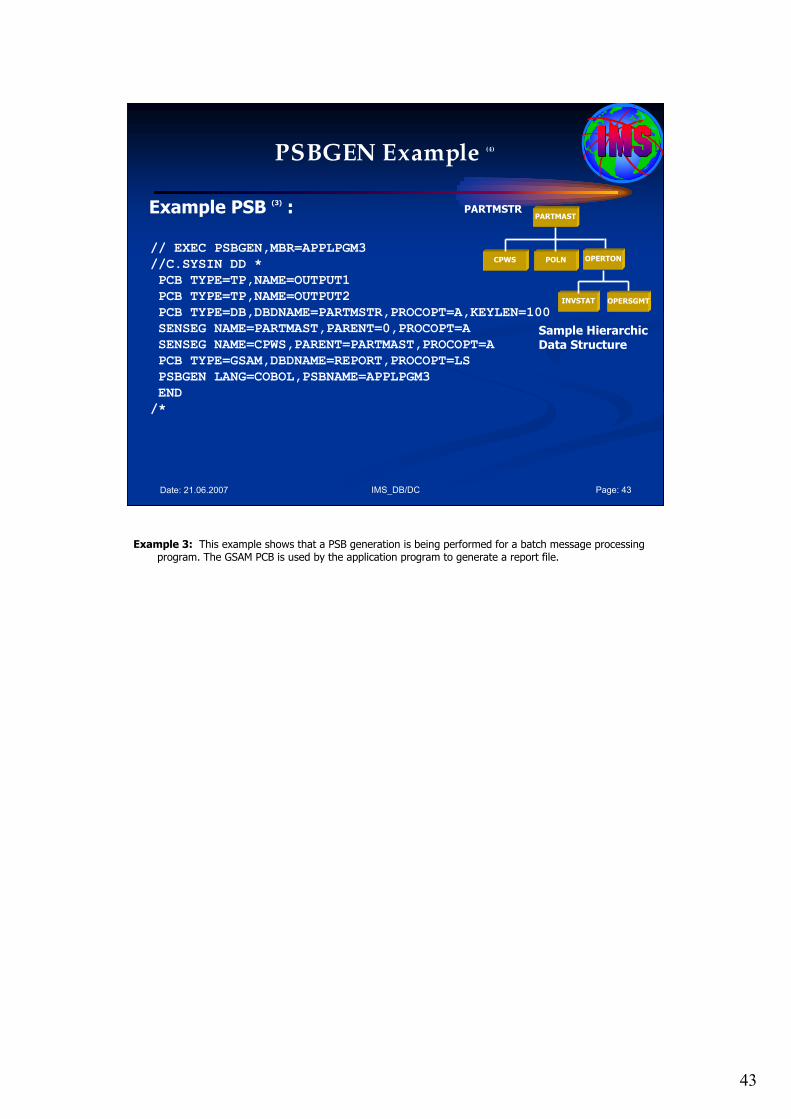
43
IMS_DB/DC Page: 43Date: 21.06.2007
PSBGEN Example (4)
PARTMAST
OPERTONCPWS POLN
OPERSGMTINVSTAT
Sample HierarchicData Structure
PARTMSTRExample PSB (3) :
// EXEC PSBGEN,MBR=APPLPGM3
//C.SYSIN DD *
PCB TYPE=TP,NAME=OUTPUT1
PCB TYPE=TP,NAME=OUTPUT2
PCB TYPE=DB,DBDNAME=PARTMSTR,PROCOPT=A,KEYLEN=100
SENSEG NAME=PARTMAST,PARENT=0,PROCOPT=A
SENSEG NAME=CPWS,PARENT=PARTMAST,PROCOPT=A
PCB TYPE=GSAM,DBDNAME=REPORT,PROCOPT=LS
PSBGEN LANG=COBOL,PSBNAME=APPLPGM3
END
/*
Example 3: This example shows that a PSB generation is being performed for a batch message processing program. The GSAM PCB is used by the application program to generate a report file.
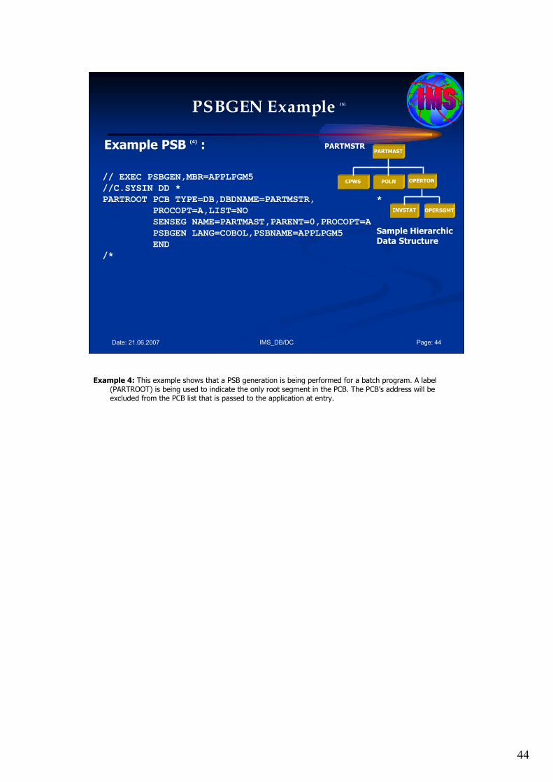
44
IMS_DB/DC Page: 44Date: 21.06.2007
PSBGEN Example (5)
PARTMAST
OPERTONCPWS POLN
OPERSGMTINVSTAT
Sample HierarchicData Structure
PARTMSTRExample PSB (4) :
// EXEC PSBGEN,MBR=APPLPGM5
//C.SYSIN DD *
PARTROOT PCB TYPE=DB,DBDNAME=PARTMSTR, *
PROCOPT=A,LIST=NO
SENSEG NAME=PARTMAST,PARENT=0,PROCOPT=A
PSBGEN LANG=COBOL,PSBNAME=APPLPGM5
END
/*
Example 4: This example shows that a PSB generation is being performed for a batch program. A label (PARTROOT) is being used to indicate the only root segment in the PCB. The PCB’s address will be excluded from the PCB list that is passed to the application at entry.
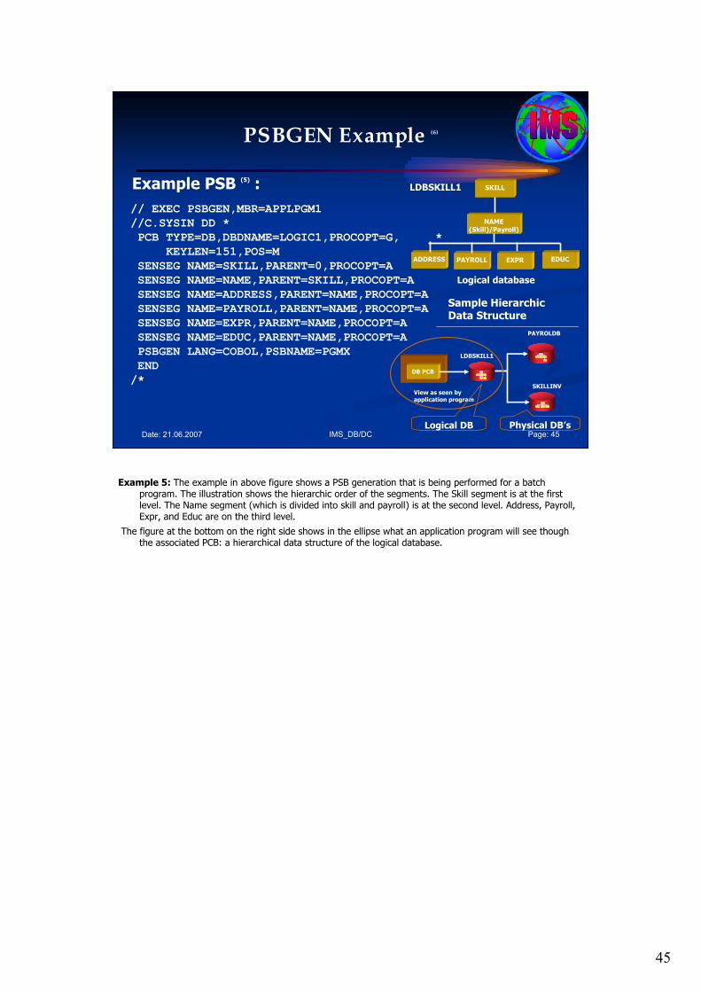
45
IMS_DB/DC Page: 45Date: 21.06.2007
PSBGEN Example (6)
Example PSB (5) :
Sample HierarchicData Structure
SKILL
NAME(Skill)/Payroll)
EXPRPAYROLLADDRESS EDUC
LDBSKILL1
Logical database
// EXEC PSBGEN,MBR=APPLPGM1
//C.SYSIN DD *
PCB TYPE=DB,DBDNAME=LOGIC1,PROCOPT=G, *
KEYLEN=151,POS=M
SENSEG NAME=SKILL,PARENT=0,PROCOPT=A
SENSEG NAME=NAME,PARENT=SKILL,PROCOPT=A
SENSEG NAME=ADDRESS,PARENT=NAME,PROCOPT=A
SENSEG NAME=PAYROLL,PARENT=NAME,PROCOPT=A
SENSEG NAME=EXPR,PARENT=NAME,PROCOPT=A
SENSEG NAME=EDUC,PARENT=NAME,PROCOPT=A
PSBGEN LANG=COBOL,PSBNAME=PGMX
END
/* DB PCB
PAYROLDB
SKILLINVView as seen by application program
LDBSKILL1
Logical DB Physical DB’s
Example 5: The example in above figure shows a PSB generation that is being performed for a batch program. The illustration shows the hierarchic order of the segments. The Skill segment is at the first level. The Name segment (which is divided into skill and payroll) is at the second level. Address, Payroll, Expr, and Educ are on the third level.
The figure at the bottom on the right side shows in the ellipse what an application program will see though the associated PCB: a hierarchical data structure of the logical database.
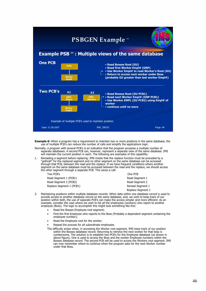
46
IMS_DB/DC Page: 46Date: 21.06.2007
PSBGEN Example (7)
Example PSB (6) : Multiple views of the same database
EMPL
WorkerEmpl#
One PCB
EMPL(Boss)
WorkerEmpl#
EMPL(Worker)
Two PCB’s #1 #2
• Read Bosses Root (GU)• Read first Worker Empl# (GNP)• Use Worker Empl# to read Worker’s Root (GU)• Return to access next worker under Boss (probably GU greater than last worker Empl#)
• Read Bosses Root (GU PCB1)• Read next Worker Empl# (GNP PCB1)• Use Worker EMPL (GU PCB2) using Empl# of worker• continue until no more
Example of multiple PCB’s used to maintain position.
Example 6: When a program has a requirement to maintain two or more positions in the same database, the use of multiple PCB’s can reduce the number of calls and simplify the applications logic.
Normally, a program with several PCB’s is an indication that the program accesses a multiple number of separate databases. A second PCB can, however, represent a separate view of the same database. IMS will maintain the current position in each. The following are examples of this capability:
1. Rereading a segment before replacing: IMS insists that the replace function must be preceded by a “gethold” for the replaced segment and no other segment on the same database can be accessed through that PCB, between the read and the replace. If we have frequent conditions where another segment on the same database must be accessed between the read and the replace, we should access the other segment through a separate PCB. This saves a call:
Two PCB’s One PCB
Read Segment 1 (PCB1) Read Segment 1
Read Segment 2 (PCB2) Read Segment 2
Replace Segment 1 (PCB1) Reread Segment 1
Replace Segment 1
2. Maintaining positions within multiple database records: When data within one database record is used to provide access to another database record on the same database, and, we wish to keep track of our position within both, the use of separate PCB’s can make the access simpler and more efficient. As an example, consider the case where we wish to list all the employees (workers) who report to another employee (Boss). The logic to accomplish this might look something like this:
• Read the Bosses Employee root segment;
• Find the first Employee who reports to the Boss (Probably a dependent segment containing the employee number);
• Read the Employee root for the worker;
• Repeat the process for all subordinate employees.
The difficulty arises when, in accessing the Worker root segment, IMS loses track of our position within the Bosses database record. Returning to retrieve the next worker for that boss is cumbersome. The solution is to establish two PCB’s for the Employee database (as shown in above figure). One is used to access the Boss and the worker Employee numbers within the Bosses database record. The second PCB will be used to access the Workers root segment. IMS can now remember where to continue when the program asks for the next Worker number under that Boss.
47
IMS_DB/DC Page: 47Date: 21.06.2007
Agenda
Session 7: Implementing IMS Databases
1. Basic Terms
2. DBDGEN
• Physical DB’s
• Logical DB’s
3. PSBGEN
4. ACBGEN
4. ACBGEN
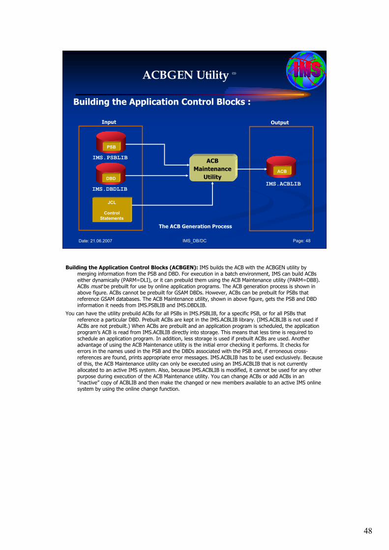
48
IMS_DB/DC Page: 48Date: 21.06.2007
ACBGEN Utility (1)
Building the Application Control Blocks :
PSB
IMS.PSBLIB
IMS.ACBLIB
ACB
ACB
Maintenance
Utility
The ACB Generation Process
Input Output
DBD
IMS.DBDLIB
JCL
Control
Statements
Building the Application Control Blocks (ACBGEN): IMS builds the ACB with the ACBGEN utility by merging information from the PSB and DBD. For execution in a batch environment, IMS can build ACBseither dynamically (PARM=DLI), or it can prebuild them using the ACB Maintenance utility (PARM=DBB). ACBs must be prebuilt for use by online application programs. The ACB generation process is shown in above figure. ACBs cannot be prebuilt for GSAM DBDs. However, ACBs can be prebuilt for PSBs that reference GSAM databases. The ACB Maintenance utility, shown in above figure, gets the PSB and DBD information it needs from IMS.PSBLIB and IMS.DBDLIB.
You can have the utility prebuild ACBs for all PSBs in IMS.PSBLIB, for a specific PSB, or for all PSBs that reference a particular DBD. Prebuilt ACBs are kept in the IMS.ACBLIB library. (IMS.ACBLIB is not used if ACBs are not prebuilt.) When ACBs are prebuilt and an application program is scheduled, the application program’s ACB is read from IMS.ACBLIB directly into storage. This means that less time is required to schedule an application program. In addition, less storage is used if prebuilt ACBs are used. Another advantage of using the ACB Maintenance utility is the initial error checking it performs. It checks for errors in the names used in the PSB and the DBDs associated with the PSB and, if erroneous cross-references are found, prints appropriate error messages. IMS.ACBLIB has to be used exclusively. Because of this, the ACB Maintenance utility can only be executed using an IMS.ACBLIB that is not currently allocated to an active IMS system. Also, because IMS.ACBLIB is modified, it cannot be used for any other purpose during execution of the ACB Maintenance utility. You can change ACBs or add ACBs in an “inactive” copy of ACBLIB and then make the changed or new members available to an active IMS online system by using the online change function.

49
IMS_DB/DC Page: 49Date: 21.06.2007
ACBGEN Examples (1)
Example (1) :
//STEP EXEC ACBGEN,SOUT=A
//SYSIN DD *
BUILD PSB=ALL
/*
Example of Creating Blocks for All PSBs
Example 1 - Example of Creating Blocks for All PSBs: In this example, all blocks currently existing in IMS.ACBLIB are deleted and their space is reused to create new blocks for all PSBs that currently reside in IMS.PSBLIB. This option will normally be used for initial creation of the IMS.ACBLIB data set. If space is not yet allocated for ACBLIB, there should be a space parameter and a DISP=NEW on the IMSACB DD statement.

50
IMS_DB/DC Page: 50Date: 21.06.2007
ACBGEN Examples (2)
Example (2) :
//STEP EXEC ACBGEN,SOUT=A,COMP=POSTCOMP
//SYSIN DD *
BUILD PSB=(PSB1,PSB2,PSB3)
DELETE DBD=(DBD5,DBD6)
/*
Example of Creating Blocks for Specific PSBs
Example 2 - Example of Creating Blocks for Specific PSBs: This example creates blocks for PSB1, PSB2, and PSB3. All other PSBs in IMS.ACBLIB remain unchanged. If any DBDs referenced by these PSBs do not exist in IMS.ACBLIB, they are added. In addition, DBD5 and DBD6 are deleted from ACBLIB. IMS.ACBLIB is compressed after the blocks are built, and deletions are performed.

51
IMS_DB/DC Page: 51Date: 21.06.2007
ACBGEN Examples (3)
Example (3) :
Example of Deleting a PSB and Rebuilding Blocks
//STEP EXEC ACBGEN,SOUT=A,COMP='PRECOMP,POSTCOMP‘
//SYSIN DD *
DELETE PSB=PSB1
BUILD DBD=DBD4
/*
Example 2 - Example of Deleting a PSB and Rebuilding Blocks: This example deletes PSB1 from the IMS.ACBLIB data set and causes all PSBs in the IMS.ACBLIB data set that reference DBD4 to have their blocks rebuilt. If PSB1 referenced DBD4, it will not be rebuilt, since PSB1 had just been deleted from IMS.ACBLIB. PSB1 is not deleted from IMS.PSBLIB. The IMS.ACBLIB is compressed before and after the blocks have been built.

52
IMS_DB/DC Page: 52Date: 21.06.2007
Source
See: • IBM Web page
http://www-306.ibm.com/software/data/ims/
• BookAn Introduction to IMS, IBM Press
In all sessions I like to motivate you to study additional books and publications about IMS DB/DC.

53
Date: 21.06.2007 IMS_03_7.ppt Page: 53
Questions / CommentsQuestions / Comments……
? ? ?? ? ?
Questions, comments, further information?
Please feel free to e-mail me!
Dipl.Ing. Werner HoffmannDipl.Ing. Werner Hoffmann
EMAIL: EMAIL: pwhoffmann@[email protected]
The time for this session is over. If you have additional questions or comments or like to get further information please feel free to e mail me at [email protected] or [email protected].

54
IMS_DB/DC Page: 54Date: 21.06.2007
The End…
Part III/7: IMS Hierarchical Database ModelIMS Hierarchical Database Model
Implementing IMS DatabasesImplementing IMS Databases
Workshop
The world depends on it
I hope this presentation was right for you! Enjoy the following discussion!